-Regularized ICA: A Novel Method for Analysis of Task-related fMRI Data
Abstract
We propose a new method of independent component analysis (ICA) in order to extract appropriate features from high-dimensional data. In general, matrix factorization methods including ICA have a problem regarding the interpretability of extracted features. For the improvement of interpretability, it is considered that sparse constraint on a factorized matrix is helpful. With this background, we construct a new ICA method with sparsity. In our method, the -regularization term is added to the cost function of ICA, and minimization of the cost function is performed by difference of convex functions algorithm. For the validity of our proposed method, we apply it to synthetic data and real functional magnetic resonance imaging data.
Keywords: independent component analysis, sparse matrix factorization, sparse coding, difference of convex functions algorithm, functional magnetic resonance imaging
1 Introduction
In machine learning, matrix factorization (MF) is known as significant unsupervised learning method for feature extraction from data, and various methods of MF have been proposed. In MF, two factorized matrices and are computed from an observed data matrix , which are related by . As the methods of MF, various independent component analysis (ICA) [1], principal component analysis (PCA), and non-negative MF [2] are widely known and frequently used. However, these MF methods have a common problem in the application to high-dimensional data: it is generally difficult to interpret what extracted features mean. To resolve this problem, sparse MF methods [3], [4] are considered to be useful, where a sparse constraint is imposed on either factorized matrix or . By introducing sparse constraint into PCA [5], [6] or non-negative MF [7], it is found that the extracted feature can be interpreted relatively easily due to sparsity. However, as far as the authors know, the widely-accepted sparse method for ICA has not been established yet.
Due to its significance, there are many applications of MF to real-world data. Analysis of biological data such as neuronal activity or electrocardiogram is one of such applications. Among various MF methods and applications, we especially focus on the application of ICA to functional magnetic resonance imaging (fMRI) data. Nowadays, fMRI is a significant experimental method for understanding the function of the whole human brain. In fMRI, time series data of cerebral blood flow in test subject is measured by magnetic resonance imaging. There are two types of fMRI: one is resting-state fMRI, which is measured under no human’s task or stimulus, and the other is task-related fMRI, which is measured under some tasks or stimuli. In the application of MF to fMRI [8], [9], [10], [11], the dimensions and are the numbers of voxels and scanning time steps, respectively. In this setting, vectors in the spatial feature factorized matrix and temporal feature matrix are interpreted as features in the human brain activity.
For feature extraction from task-related fMRI by MF, it is considered that statistical independence among extracted feature signals is generally significant, in particular for temporal feature matrix . However, it will be better to impose an additional constraint such as sparsity on spatial feature matrix for localization of the elements in . This is because it is widely believed that information representation for external stimuli in the human brain is sparse. Therefore, it is not enough for feature extraction only to assume statistical independence for temporal feature . Practically, in the application of ICA to fMRI data, statistical independence is often imposed on instead of for localization of elements in . Such ICA is specifically called spatial ICA [12]. In contrast, the method with the assumption of statistical independence on temporal feature is called temporal ICA. In this connection, it is shown recently that sparse MF or spatial ICA can extract more appropriate features from fMRI data than other MF methods without localization of the elements in [13]. From these facts, we expect that temporal ICA can be improved by adding a sparse constraint on the matrix .
With this background, we propose a novel ICA method, which may extract features appropriately from task-related fMRI. In our method, we minimize the cost function of ICA with an additional regularization term. Namely, we impose the constraints of statistical independence on and sparsity on . For minimizing the proposed cost function, we apply difference of convex functions (DC) algorithm [14, 15, 16], which is a powerful tool in nonconvex optimization problem.
The organization of this article is as follows. In section 2, the framework of ICA is overviewed and several related works are presented. In section 3, we provide how to construct our proposed method and discuss the convergence of our algorithm theoretically. In section 4, we apply our method both to synthetic data and real-world data, then discuss the validity. Finally, section 5 is devoted to conclusions and future works.
2 Overview of ICA
Throughout this article, matrices are denoted by bold uppercase letters such as and vectors as bold lowercase letters such as . Scalars are denoted as small italic, and elements of vector/matrix are written as italic lowercase letter such as .
2.1 Framework of ICA and FastICA
In the introduction, we mainly focus on the application of ICA to fMRI. In practice, ICA is applied not only to biological data analysis but also to other various problems such as image processing or finance. Therefore, we formulate our proposed ICA in general setting for the application to various problems.
Originally, ICA is proposed as one of the blind source separation methods. The objective of all ICA methods is to estimate latent independent source and mixing matrix simultaneously without any prior knowledge on them. In many algorithms of ICA, non-gaussianity is the quantity to be maximized.
Among various ICA methods, FastICA [17] is a widely used algorithm. In FastICA, factorized matrices are estimated as follows.
-
1.
The observed matrix is prewhitened by as , where denotes the prewhitening matrix and denotes the prewhitened observed matrix.
-
2.
Next, the projection matrix is evaluated, which maximizes non-gaussianity among rows of the signal source matrix . The projection matrix is frequently called unmixing matrix. The cost function for non-gaussianity is defined by
(1) In the above equation, is a nonlinear function and defined by . The variable ) is a normal random variable with zero mean and unit variance. In maximizing , a fixed point algorithm in equation (2) is used.
(2) In addition, the orthogonal constraint is imposed on the projection matrix , where is -dimensional identity matrix. In practice, the column vectors of are mutually orthogonalized by Gram-Schmidt method, where the column vectors are updated as follows,
(3) -
3.
The mixing matrix is calculated as , where is Moore-Penrose pseudo-inverse matrix of . Accordingly, the observed matrix , the mixing matrix , and signal source matrix are related by , which is shown by the orthogonality of .
2.2 Related works on ICA with sparse constraint
Before going into our proposed method, we should mention several related works regarding ICA with sparse constraint. First, there is a method called SparseICA [18], [19], which was introduced for blind source separation in image processing in real-world application [20]. In this method, independent source matrix is computed as the product of the sparse coefficient matrix and the dictionary matrix by .
Next, ICA with regularization terms was proposed for the linear non-gaussian acyclic model [21]. In this method, the regularization term for the separation matrix defined by is introduced. It should be noted that the construction of sparse matrix in ICA is similar to our proposed method explained in the following section. However, the sparse constraint on the matrix is different. In this method, the sparse constraint is imposed on the separation matrix , while the estimated mixture matrix is sparse in our method. Similar studies with sparse separation matrix can also be found in other references [22], [23].
There is also other related work [24], where the sparse constraint is imposed on the mixing matrix like our method. Additionally, the objective of the work is to identify sparse neuronal networks like ours. However, there is a difference in the methodology: this method is based on Bayesian framework and the algorithm is a stochastic one. More precisely, the mixing matrix and parameters in the model are assumed to follow some probabilistic distributions and optimized by Markov chain Monte Carlo method. In contrast, our method is a deterministic one, where the cost function is minimized by DC algorithm.
3 Our method
In this section we elucidate the detail of our proposed method.
3.1 Formulation
In our method, the -th vector in the projection matrix minimizing cost function in equation (4) must be evaluated.
| (4) |
Here is -norm, , and is given by the minimizer in equation (5).
| (5) |
with being Frobenuis norm and being the matrix -norm or the number of non-zero elements in the matrix, respectively. By definition, the minimizer matrix is close to the original and sparse with only nonzero elements. We need the sparse estimated mixture matrix , whose sparsity depends on the sparsity of [25]. Hence, approximate sparse inverse whitening matrix is favorable rather than the original inverse whitening matrix in our proposed method. In practical computation, the algorithm of orthogonal matching pursuit [26], [27] is applied to obtain each row of .
We apply widely-used DC algorithm for minimization of the cost function. DC algorithm is applicable to the minimization problem, where the cost functions is represented by the difference of two convex functions as
| (6) |
Note that Hessians of the two convex functions must be bounded above. In DC algorithm, the following two processes are repeated until convergence or maximum iteration number is reached.
-
(i)
Update by choosing one element from the subgradient set of , namely with being the -th update of .
-
(ii)
Update by .
It is considered that the convergent solution by DC algorithm is often a global optimal solution. Therefore, DC algorithm is one of the effective approaches for nonconvex optimization.
For application of DC algorithm to minimization in our method, the cost function must be expressed by the difference of two convex functions. First, Lipschitz constant of is introduced, which can be defined because is secondary differentiable. Then, the function is easily proved to be convex by the definition of Lipschitz constant . Moreover, regularization term is clearly convex, and the sum of two convex functions is also convex. Therefore, can be represented by the difference of two convex functions like , where the two convex functions are defined in equations (7) and (8).
| (7) | |||||
| (8) |
Note that and are continuous functions in our -regularized ICA.
In DC algorithm, computation of Lipschitz constant needs maximum eigenvalue of Hessian , whose computational complexity is . In practice, is evaluated by backtracking line search algorithm [28]. In this algorithm, we prepare the tentative Lipschitz constant in the -th update, then is accepted as the final Lipschitz constant if the criterion of inequality (9) is satisfied for . Otherwise, is rescaled by with the constant , then inequality (9) is checked again.
| (9) |
After evaluation of Lipschitz constant, we move on to the formulation of DC algorithm in our proposed method. In DC algorithm, subderivative is necessary for the calculation of in the process (i), which is given by equation (10),
| (10) |
Then, the process (ii) for the update of is represented as follows.
| (11) |
The minimization problem in equation (11) can be regarded as a generalized lasso problem [29], whose solution cannot be obtained analytically. Hence, we attempt to find the solution numerically by the method of alternating directions method of multipliers (ADMM) [30]. In the application of ADMM, is computed by minimizing augmented Lagrangian ,
| (12) |
The variables minimizing are alternately updated by equations (13), (14) and (15) until convergence.
| (13) | |||||
| (14) | |||||
| (15) |
where superscript means the variable of the -th update in ADMM iteration. Update of can be rewritten by putting the solution of , which leads to
| (16) |
Similarly, by solving equation analytically, update of the -th element in is represented as follows,
| (17) |
where means the -th row vector of and is soft thresholding function defined in equation (18),
| (18) |
Finally, by combining these results, our proposed algorithm is obtained, which is summarized in Algorithm 1.
3.2 Convergence analysis
We can derive a convergence condition for our proposed algorithm for -regularized ICA. The theorem and the proof of the convergence condition are given in the following.
For general DC algorithm, the condition of non-increasing function must be satisfied for the updated variable [31]. When this condition is satisfied, it is guaranteed that the sequence converges to a point satisfying the condition for subgradient as
| (19) |
The significant difference of DC algorithm in our -regularized ICA is orthogonalization and normalization after variable update, which requires a slight change in the proof for convergence condition of DC algorithm. For this purpose, we should distinguish the variable after orthogonalization and normalization, which is denoted by . With this variable, we can show that our proposed algorithm converges to a point in equation (19) if the inequality is satisfied.
The convergence theorem for our proposed algorithm is stated as follows. It should be commented that the convergence condition in the theorem is a sufficient condition, which can be relaxed.
Theorem 1.
If the following condition is satisfied at each step of , the sequence converges to a certain point by our proposed algorithm.
| (20) |
where is a constant defined by
| (21) | |||||
In this definition, the operation of orthogonalization is expressed by the multiplication of a square matrix , namely , and are maximum and minimum eigenvalues of square matrix in the parenthesis, respectively.
Proof.
From the convexity of the function ,
| (22) |
The -th vector is orthogonalized to the set of vectors first, then normalized. After orthogonalization, the normalized vector is calculated as . For this vector , the upper bound of is estimated as
| (23) | |||||
where the constant is determined by the upper bounds of the following terms,
, , and . These three terms can be bounded as follows.
| (24) |
| (25) | |||||
Note that the factor on the right hand side of inequality (LABEL:eq:upper_bound_of_3rd_term) is cosine similarity. The inequality in (24) is from the upper bound of the general quadratic form. The first inequality in (25) is derived by the relation between -norm and -norm, namely for an -dimensional vector , and the second inequality is from the upper and the lower bounds of the general quadratic form. The inequality in (LABEL:eq:upper_bound_of_3rd_term) is Cauchy-Schwarz inequality. By these results and from the definition of in (11), the last inequality in (23) is shown using the constant in (21). Then, if the condition (20) is satisfied, one has
| (27) | |||||
This means the property is proved, which guarantees the convergence. ∎
4 Numerical experiment
4.1 Application to synthetic data
For validity of our proposed method, we apply our method to synthetic data to evaluate its performance. In addition, we compare the performance of our method with widely-used FastICA algorithm. In our numerical experiments, we use scikit-learn library (version 1.2.2) for Python (version 3.10.11).
Experimental conditions and performance measure
In this experiment, we apply our proposed method and FastICA to 4 synthetic data , , and , which are generated as follows. In particular, in constructing and , the values of parameters are chosen to model large-size real fMRI data. (See also Table 1.)
| data | dist. of | dist. of | ||
|---|---|---|---|---|
| 80% uniform, 20% Laplace | 10 | 0.8 | ||
| 80% uniform, 20% log-normal | 10 | 0.8 | ||
| 80% uniform, 20% log-normal | 0.999 | |||
| 80% uniform, 20% log-normal | 0.999 |
-
1.
First, the ground-truth signal source matrix is generated, whose elements are drawn from Laplace distribution, log-normal distribution, or uniform distribution defined by
(28) (29) (30) Note that these distributions are non-gaussian distributions. For constructing , 20% of the vectors in have elements following Laplace distribution and 80% have elements following uniform distribution. Similarly, 20% of the vectors in have elements following log-normal distribution and 80% have elements following uniform distribution for , and . For all synthetic data, the dimensions of are set as .
-
2.
Next, the ground-truth mixing matrix is generated, whose element is drawn from Bernoulli-gaussian distribution.
(31) For and , we set , namely the size of the data is small. In contrast, we set for and to model real fMRI data, because the voxel size of fMRI data often takes the order from to . Moreover, in real fMRI data analysis as mentioned in section 4.2, elements of brain activity above 3 standard deviations from the mean can be interpreted as clear characteristic activations. Namely, the number of elements representing strong activations is typically of the order of . From this observation, we set for and .
-
3.
The observed matrix is constructed from and by the matrix product , where is noise matrix with the elements following standard gaussian distribution for , and . For , the element of noise matrix follows , namely noisier case.
After application of our proposed method to the synthetic matrix , the result is evaluated by the performance measures in the following.
-
•
sparsity
Sparsity of the estimated mixture matrix is defined in equation (32).(32) where is the -element of normalized and is the indicator function. In our experiment, we set the infinitesimal threshold . Under experimental condition mentioned above, the sparsity of the ground-truth mixture matrix is 0.8 after truncation of the elements.
-
•
kurtosis
For non-gaussianity, mean of absolute values of kurtosis (denoted by MAK) for the estimated signal matrix is used,(33) which is zero for the matrix with the elements following gaussian distribution.
-
•
RMSE as the reconstruction error
For validity as an MF solution, rooted mean squared error (RMSE) is defined between the original observed matrix and the product of estimated matrices for describing reconstruction error.(34) -
•
reconstruction success rate
In general MF problem including ICA, the matrices after permutation of vectors in factorized matrix solution are also another solution. Therefore, it is not appropriate to measure RMSE between the ground-truth mixing matrix and estimated mixing matrix directly. To evaluate the difference between and by considering permutation symmetry of MF solution, Amari distance [32] is defined to measure how the product is close to the permutation matrix as(35) Amari distance is regarded as a significant performance measure in ICA, because it is known that is equivalent to the permutation matrix if signal sources can be separated perfectly. When an algorithm of ICA is executed in trials under given observed matrix and different initial matrix , the reconstruction success rate is defined using Amari distance,
(36) where the superscript means the -th trial.
In our experiment, these quantities are evaluated under various and the sparsity of . For simplicity, the sparsity of is denoted by in the following. The parameters other than and are fixed as follows: . Sparsity, kurtosis, and RMSE are evaluated by our algorithm in 10 trials under the same observed matrix and different initial matrix . Statistical error of multiple trials is shown by the error bar in the figures.
Result 1: General property of factorized matrices by the proposed method
We depict the behaviours of the sparsity of the estimated mixture matrix , the kurtosis of the estimated signal matrix , and the reconstruction error obtained by our proposed method and FastICA in Figure 1. The results for (top, under the mixtures of Laplace/uniform distributions) and (bottom, log-normal/uniform distributions) are compared. From this figure, there is no significant difference between mixtures of Laplace/uniform distributions and log-normal/uniform distributions. This implies that the result does not depend on the choice of non-gaussian distribution.
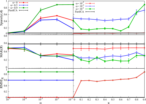
We move on to the detail of the results in Figure 1. First, we discuss the sparsity of the estimated mixture matrix . The sparsity of by our proposed method is larger than FastICA regardless of the value of . We also observe that the sparsity by our method is very large and close to 0.9 under larger and . When the value of is fixed, large sparsity is obtained for large under or . In general, must be larger for larger sparsity of , while should be tuned carefully.
Next, we observe the behavior of . by our method tends to decrease for larger , while by FastICA does not. This may be because our ICA solution under larger is different from the solution of the conventional FastICA. On the other hand, there is no significant correlation between and . Therefore, for larger non-gaussianity, can take arbitrary value, while should be appropriately adjusted.
We also mention the result of the reconstruction error. In Figure 1, no change in is observed even if is varied, and depends only on . It is easy to prove analytically that depends only on the approximation accuracy of using the orthogonality of the matrix , which is also indicated by numerical result. In addition, by fixing , it is found that tends to increase for larger . To summarize, can be chosen arbitrarily for better reconstruction error, while must be carefully adjusted. Additionally, from the fact that larger sparsity of can be obtained under larger , large sparsity and small reconstruction error have a trade-off relation.
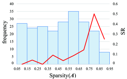
Lastly, we give the result of the reconstruction success rate. Before evaluating SR of our method, we evaluate Amari distance by FastICA in 20 trials with different initial matrix, whose average is . Based on this result, the threshold of success is set as in our experiment, which is the appropriate value because it is below the average of Amari distance by FastICA. For reconstruction success rate, we evaluate it in 20 trials with different initial matrix for . Parameter is set to 0.9 in all cases. In Figure 2, we show the frequency of samples and SR under various sparsity of estimated matrix . The largest SR is observed in the range of . As stated in the experimental conditions, the sparsity of the ground-truth mixture matrix is 0.8. Therefore, this result indicates that the ground-truth mixture matrix can be obtained by our method with high probability, especially when the sparsity of is close to the one of .
Result 2: Application to large synthetic data modelling fMRI
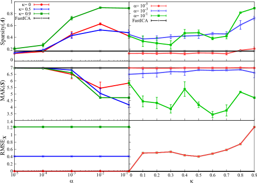
We also apply our method and FastICA to synthetic data and , which model real fMRI data with larger dimension. Similar to the applications to and , the behaviors of the sparsity of , the kurtosis of , and the reconstruction error are depicted in Figure 3.
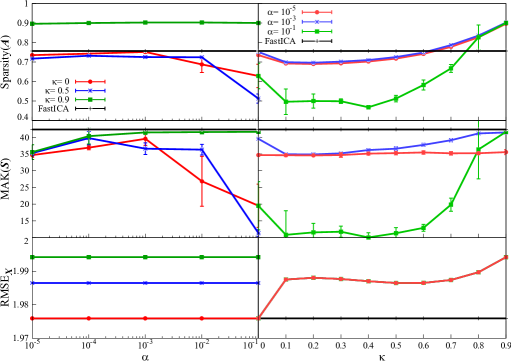
The result is summarized as follows. First, sparsity of is almost unchanged even when is varied, especially in applying to . As for the dependence on , sparsity takes a large value at , and it suddenly decrease then gradually tends to increase when is increased from . In the application of -regularized MF, similar phenomenon of little change in sparsity when varying has already been observed in the previous study [33]: if synthetic data is generated by very sparse ground-truth factorized matrix , application of SparsePCA does not significantly change the sparsity of the resulting factorized matrix even when the sparse parameter in SparsePCA is varied. Since the evaluation of sparsity here is performed similarly to SparsePCA in the previous study, we guess that similar behavior of sparsity is obtained in this experiment. In the application to , the change of sparsity depends on rather than , which is similar to . Note that the sparsity by FastICA is not so large in this case, while our method can sparsify factorized matrix. This indicates the validity of our method to obtain sparse factorized matrix from noisy large-size data.
Next, for , there is no clear trend between kurtosis of and both of sparse parameters , while the statistical error of kurtosis is very large under excepting the point . This result suggests that parameters should be tuned carefully for the stable solution with large kurtosis, if the data is less noisy. In contrast, for , kurtosis tends to increase from to 0.9. From this result, should be larger for larger kurtosis, when our method is applied to noisy large-size data.
The behavior of reconstruction error is similar to Figure 1, while its value is much larger than those in Figure 1. This is caused by the fact that Moore-Penrose pseudo inverse matrix cannot approximate the true inverse matrix appropriately under , which is the problem inherent in original ICA.
Lastly, we compare the result of application to with FastICA. Before comparison with FastICA, we evaluate the sparsity and AD by FastICA in 20 trials with different initial matrix. The average of sparsity is and the average of AD is . Then, in the application of our method here, the parameter is set to be , and the experiment is conducted in 20 trials with different initial matrix for each value of (totally 60 trials). The parameter is fixed at . Table 2 shows the result by our method. The threshold in the definition of SR is set at for comparison with FastICA. This result in the table suggests that the factorized matrix with lower AD than FastICA can be obtained with approximately 50% probability, when the sparsity is larger than FastICA. Namely, our proposed method can obtain a closer factorized matrix to the ground-truth mixing matrix than FastICA at a certain probability. This suggests that our method is competitive with original FastICA for evaluating of sparse and independent factorized matrices from large-size noisy data. As written in section 4.2, it should be emphasized that the validity of our method for application to fMRI data will be discussed.
| sparsity | frequency | SR |
|---|---|---|
| smaller than FastICA | 19 | 0.211 |
| larger than FastICA | 41 | 0.488 |
4.2 Application to real-world data
Next, for verifying the practical utility of our method, we conduct an experiment for feature extraction in real fMRI data.
Dataset and performance measure
We apply our method to Haxby dataset [34], which is a task-related fMRI dataset recording human’s response to 8 images. The 8 images are as follows: shoe, house, scissors, scrambledpix, face, bottle, cat, and chair. In the experiment of fMRI data acquisition, one image is shown to a test subject for a while, then the next image is shown after an interval. Finally, all 8 images are shown sequentially. The whole Haxby dataset includes fMRI data of 12 trials from 6 test subjects. The previous study [13] shows no significant difference among subjects in this dataset. Therefore, in our experiment, we apply our method and FastICA to one trial data of test subject No. 2, which was acquired from 39912 voxels with 121 scanning time steps. In our experiment, we apply our method and FastICA to one trial data from the test subject No. 2, which was acquired from 39912 voxels with 121 scanning time steps. Namely, the data matrix size is or .
As performance measures, we use sparsity in equation (32) and correlation defined by
| (37) |
where overline means the arithmetic average of all elements in the vector. The vector means the -th temporal feature vector in the matrix . The column vector represents the ground-truth timing of resting state: the -th element of is 1 if no image is shown to the test subject at the -th time step, and 0 if one of the images is shown, respectively. Therefore, the quantity in equation (37) measures the correlation between the ground-truth timing vector of the resting state and temporal feature vector in .
Result
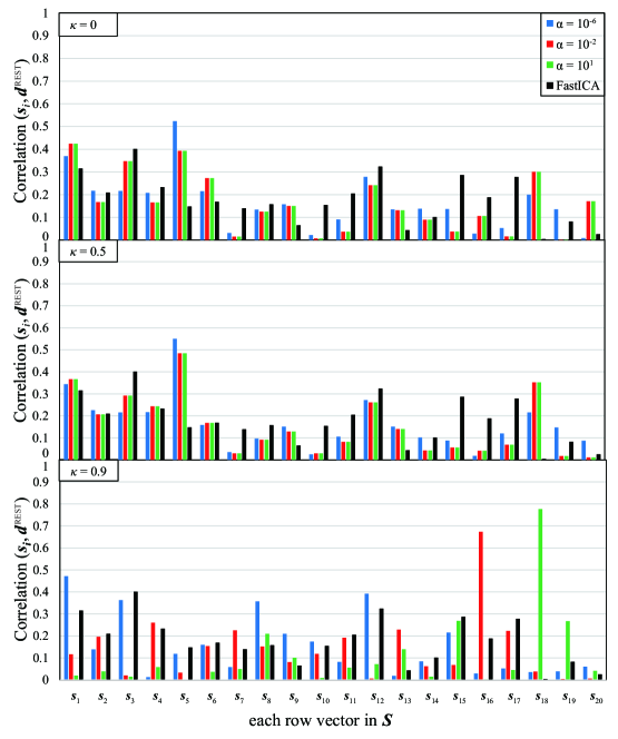
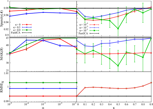
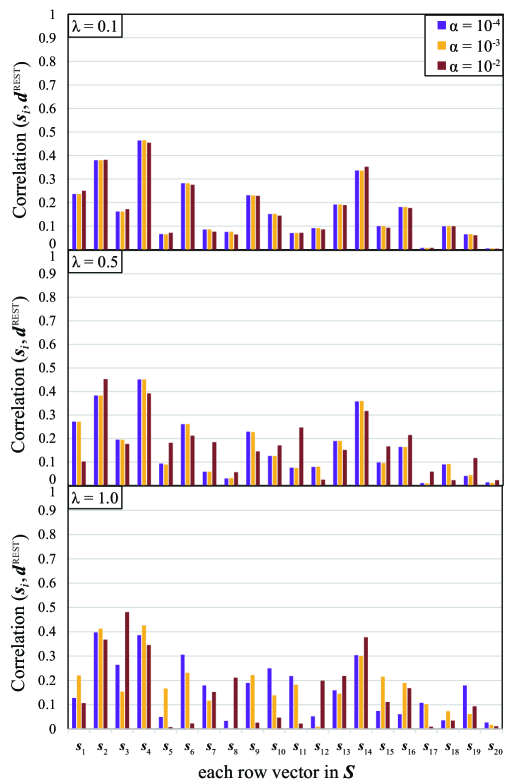
The result of correlation is depicted in Figure 4 under various : and . Other parameters are set as follows: . From this figure, the value of correlation is at most 0.6 for , whereas it sometimes exceeds 0.6 under for . In addition, to confirm the validity of our method, we apply FastICA and our proposed method under to the same data 50 times with different initial matrix, then conduct Student’s two-sample -test for the first, the second, and the third largest values of Correlation. The result is shown in Table 3, where negative value means that the Correlation by our method is larger. From this result, there is a significant difference between the results by our method and FastICA, and it is clear that the first and the second largest values of Correlation by our method are larger than FastICA. Although the third largest value by FastICA is larger, we think it is sufficient to claim the advantage of our method over FastICA.
| value of Correlation | 1st | 2nd | 3rd |
|---|---|---|---|
| t-statistic | -25.7 | -3.33 | 5.43 |
| p-value |
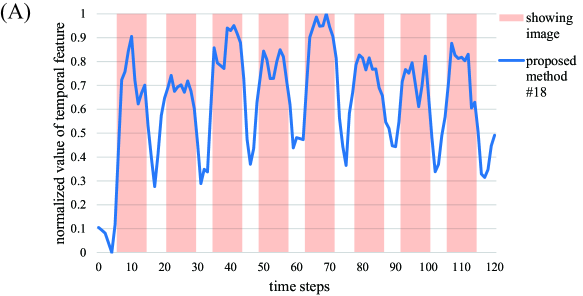
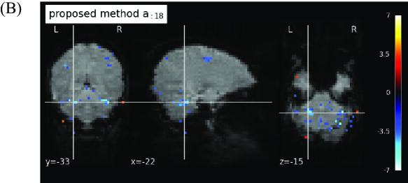
Next, we visualize the extracted feature vectors by our method. The 18th row vector in by our method under is depicted in Figure 5A. Note that the 18th row vector has the largest Correlation in our result under as shown in Figure 4. The timing of showing image to a test subject, which reflects the information of the vector , is also shown in the figure. From this result, the temporal changes between resting and non-resting states can be tracked easily in the feature vector by our method. Additionally, the spatial map of the 18th spatial feature vector in by our method is shown on the cross sections of the brain in Figure 5B. Note that this spatial feature vector is the counterpart of the 18th temporal feature vector in Figure 5A. For spatial map, the column vectors in are normalized to have zero mean and unit variance, and elements within 3 standard deviations of the mean are truncated to zero. For visualization of the spatial map, we use Nilearn (version 0.10.1) in Python library. In this figure, several active regions under resting state or the response to some visual stimuli can be observed. In particular, strong activations are observed in the cerebellum, which is known to be activated by visual stimuli. This result indicates that our method with high sparsity setting can identify brain regions for information processing of visual stimuli with high accuracy.
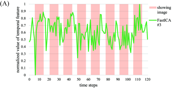
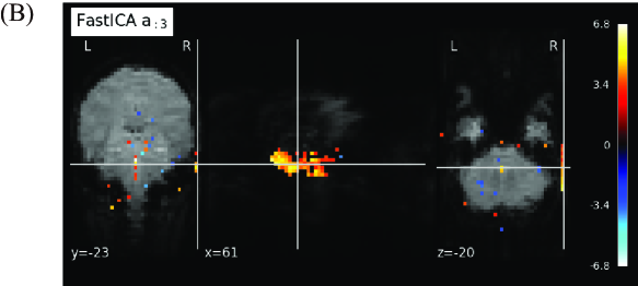
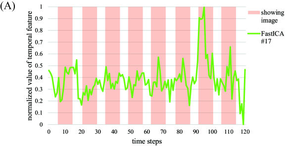
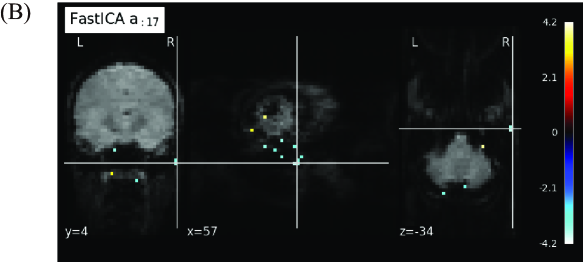
To compare our proposed method and FastICA, we show the behaviors of two feature vectors given by FastICA, namely the 3rd and the 17th vectors. For clarity, extracted feature vectors are denoted with a superscript, which represents the method for comparing FastICA and our proposed method. For example, the 3rd vector in by FastICA is written as . First, the vector and the spatial map of are depicted in Figures 6A and 6B, respectively. Note that the vector is most strongly correlated with the timing vector of visual stimuli as in Figure 4. However, from Figure 6A, resting and non-resting regions in fMRI data cannot be discriminated from the shape of the feature vector by FastICA. In addition, we cannot clearly identify which parts of the brain are strongly activated from Figure 6B. We also depict the vector and the spatial map of in Figures 7A and 7B, respectively. Note that the vector is most strongly correlated with the vector , whose counterpart has the largest value of Correlation with under appropriate as in Figure 4. For Correlation between these two column vectors, see also Figure 8A in the following. Similarly to the vector , we cannot find significant synchronization with the timing of visual stimuli from Figure 7A, and it is difficult to understand what the spatial map of means because the area of activation in the brain is not clear from Figure 7B.
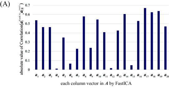
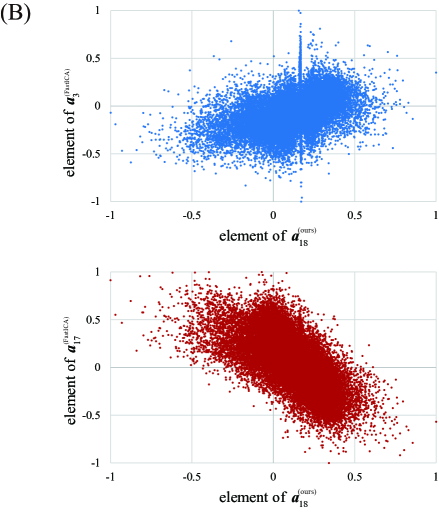
For relation between spatial maps by the two methods, we evaluate the absolute value of Correlation between the vector and each column vector of by FastICA in Figure 8A. From this result, we find that the vector is most strongly correlated with the vector . In Figure 8B, we depict the scatter plot of the element in the vector vs. the corresponding element in the vector (top) or (bottom), where the values of the elements in spatial vectors are normalized to the range by the linear transformation. From this figure, the vector is more strongly correlated with the vector . Hence, these two spatial feature vectors will represent similar spatial networks. As mentioned in the result of Figure 7, synchronization with the timing of visual stimuli is not observed in the vector , which is the counterpart of the spatial feature vector . In contrast, the temporal feature vector is clearly synchronized with the timing of visual stimuli, and the corresponding spatial feature also shows activation in the region related to visual stimuli. From these facts, we can conclude that our method outperforms FastICA in feature extraction from fMRI data.
We think the advantage of our method is due to the sparsity of the estimated mixture matrix . To support this, the sparsity of by this experiment is summarized in Table 4. From this table, it is found that the parameters giving the feature vector with the largest correlation () lead to the sparsest matrix . On the other hand, by FastICA is evaluated as 0.104, which is much smaller than our method. In the previous study [35, 36, 13], it is claimed that the method of MF giving sparse can extract appropriate temporal feature vector characterizing the external stimuli. Therefore, the result indicating the advantage of our method is consistent with the previous studies.
| 0.095 | 0.099 | 0.099 | |
| 0.098 | 0.101 | 0.101 | |
| 0.156 | 0.505 | 0.770 |
| 0.91 | 0.91 | 2.08 | |
| 1.27 | 1.41 | 1.36 | |
| 1.27 | 1.41 | 1.50 |
| 0.904 | 0.908 | 0.922 | |
| 0.904 | 0.908 | 0.922 | |
| 0.904 | 0.908 | 0.922 |
To verify the significance of sparsity, the kurtosis of the estimated temporal feature matrix and the reconstruction error by our method are also summarized in Table 4. For comparison, and obtained by FastICA are 12.37 and 0.904, respectively. Recall that the objective of this experiment is to identify the temporal features response to external stimuli. Hence, this result suggests that the sparsity of spatial features is more important than the kurtosis of temporal features or the reconstruction error in feature extraction of neuronal activity data. This fact can be reinforced by the result of previous study [13], where they applied sparse MF methods, namely SparsePCA and method of optimal directions (MOD), to the same dataset and investigated the performance of feature extraction and reconstruction error. As a result, even under the case of the large reconstruction error, appropriate features are obtained if the sparsity of the spatial feature in the brain is large. Our result of experiment shows that the accuracy of synchronization between extracted temporal features and the timing of showing images can be improved by sparsifying spatial features in the brain, even if the kurtosis of temporal features is decreased. Therefore, it can be concluded that the sparsity of spatial features in the brain is the most important to obtain features corresponding to visual stimuli.
For comparison, we also apply another sparse ICA method in the previous work [21] to the same data. In their method, the sparsity of the matrix is controlled by two parameters , and we set , respectively. The result in Figure 9 shows that very large value of Correlation over 0.5 cannot be obtained, in other words appropriate feature cannot be extracted sufficiently by the ICA method of sparsifying the matrix . In contrast, our method sparsifying the matrix yields very large value of Correlation and works more appropriately for feature extraction from fMRI data.
It should be mentioned that there is also an analysis for the same data by MOD [13]. In the previous study, it is claimed that MOD with high sparsity setting can extract the activations in the cerebellum. Comparing the results by the proposed method and MOD, it is observed that the spatial maps from the proposed method and MOD are similar. However, the maximum correlation between the temporal vector and visual stimuli (or resting states) by MOD is 0.716 under . Therefore, it can be concluded that our method has advantage over MOD under the same value of . In addition, the previous study also showed that spatial ICA and SparsePCA can extract significant features. In the spatial features extracted by these methods, strong activations are observed in the region of early visual cortex, which differ from the one obtained by MOD or our proposed method. Such differences should be interpreted as the effectiveness of all methods (MOD, SparsePCA, spatial ICA, and our method) in extracting features from neural activity data, and the comparison among these methods does not make sense so much. In conclusion, this fact also supports the validity of our method for feature extraction from fMRI data.
5 Conclusion
In this study, we propose a novel ICA method giving sparse factorized matrix by adding an regularization term. We also evaluate its performance by the application both to synthetic and real-world data. From the result by numerical experiment, we expect that the proposed method gains the interpretability of the result in comparison with the conventional ICA, because our method can give sparse factorized matrix by appropriate tuning of parameters. Furthermore, in the application to task-related fMRI data, our method can discriminate resting and non-resting states, and it is competitive with MOD or other MF methods. This indicates the utility of our proposed method in practical analysis of biological data.
As future works, we will compare the performance of our proposed method with other ICA methods, in particular stochastic ICA [24] among them. Due to its stochastic nature, it may be difficult to obtain a sparse factorized matrix stably. However, the stochastic method may have advantages over our method, for example on scalability by appropriate parameter tuning or data preprocessing. It is also necessary to apply our method to other real-world data such as genetic or financial ones, and investigate its utility. In particular, in the analysis of gene expression, it is reported that ICA with the assumption of independence on temporal features is suitable for gene clustering [37, 38]. In addition, it is known that the interpretation of gene clusters becomes easy by imposing sparsity on gene features [6]. Hence, our method will be helpful for finding a novel feature of gene expression. Finally, we hope that our method is found to be useful in various fields and can contribute to feature extraction in many practical problems.
Acknowledgments
The authors are grateful to Kazuharu Harada for sharing his related work [21] and offering program code of sparse ICA in his work. This work is supported by KAKENHI Nos. 18K11175, 19K12178, 20H05774, 20H05776, and 23K10978.
References
- [1] Pierre Comon. Independent component analysis, a new concept? Signal processing, 36(3):287–314, 1994.
- [2] Daniel Lee and H Sebastian Seung. Algorithms for non-negative matrix factorization. Advances in neural information processing systems, 13, 2000.
- [3] K. Engan, S.O. Aase, and J. Hakon Husoy. Method of optimal directions for frame design. IEEE International Conference on Acoustics, Speech, and Signal Processing. Proceedings. ICASSP99, 5:2443–2446, 1999.
- [4] Michal Aharon, Michael Elad, and Alfred Bruckstein. K-svd: An algorithm for designing overcomplete dictionaries for sparse representation. IEEE Transactions on signal processing, 54(11):4311–4322, 2006.
- [5] Ian T. Jolliffe, Nickolay T. Trendafilov, and Mudassir Uddin. A modified principal component technique based on the lasso. Journal of Computational and Graphical Statistics, 12(3):531–547, 2003.
- [6] Hui Zou, Trevor Hastie, and Robert Tibshirani. Sparse principal component analysis. Journal of computational and graphical statistics, 15(2):265–286, 2006.
- [7] Patrik O. Hoyer. Non-negative matrix factorization with sparseness constraints. J. Mach. Learn. Res., 5:1457–1469, 2004.
- [8] Surya Ganguli and Haim Sompolinsky. Compressed sensing, sparsity, and dimensionality in neuronal information processing and data analysis. Annual review of neuroscience, 35:485–508, 2012.
- [9] Xiaoyu Ding, Jong-Hwan Lee, and Seong-Whan Lee. Performance evaluation of nonnegative matrix factorization algorithms to estimate task-related neuronal activities from fmri data. Magnetic resonance imaging, 31(3):466–476, 2013.
- [10] Jinglei Lv, Binbin Lin, Qingyang Li, Wei Zhang, Yu Zhao, Xi Jiang, Lei Guo, Junwei Han, Xintao Hu, Christine Guo, et al. Task fmri data analysis based on supervised stochastic coordinate coding. Medical image analysis, 38:1–16, 2017.
- [11] Michael Beyeler, Emily L Rounds, Kristofor D Carlson, Nikil Dutt, and Jeffrey L Krichmar. Neural correlates of sparse coding and dimensionality reduction. PLoS computational biology, 15(6):e1006908, 2019.
- [12] Christian F Beckmann, Marilena DeLuca, Joseph T Devlin, and Stephen M Smith. Investigations into resting-state connectivity using independent component analysis. Philosophical Transactions of the Royal Society B: Biological Sciences, 360(1457):1001–1013, 2005.
- [13] Yusuke Endo and Koujin Takeda. Performance evaluation of matrix factorization for fmri data. Neural Computation, 36(1):128–150, 2024.
- [14] Pham Dinh Tao and El Bernoussi Souad. Algorithms for solving a class of nonconvex optimization problems. methods of subgradients. In J.-B. Hiriart-Urruty, editor, Fermat Days 85: Mathematics for Optimization, volume 129 of North-Holland Mathematics Studies, pages 249–271. North-Holland, 1986.
- [15] Pham Dinh Tao and El Bernoussi Souad. Duality in dc (difference of convex functions) optimization. subgradient methods. In Trends in Mathematical Optimization: 4th French-German Conference on Optimization, pages 277–293. Springer, 1988.
- [16] Le Thi Hoai An and Pham Dinh Tao. The dc (difference of convex functions) programming and dca revisited with dc models of real world nonconvex optimization problems. Annals of operations research, 133:23–46, 2005.
- [17] Aapo Hyvärinen and Erkki Oja. Independent component analysis: algorithms and applications. Neural networks, 13(4-5):411–430, 2000.
- [18] Michael Zibulevsky, Pavel Kisilev, Yehoshua Zeevi, and Barak Pearlmutter. Blind source separation via multinode sparse representation. Advances in neural information processing systems, 14, 2001.
- [19] Michael Zibulevsky and Barak A. Pearlmutter. Blind source separation by sparse decomposition in a signal dictionary. Neural Computation, 13(4):863–882, 2001.
- [20] Alexander M Bronstein, Michael M Bronstein, Michael Zibulevsky, and Yehoshua Y Zeevi. Sparse ica for blind separation of transmitted and reflected images. International Journal of Imaging Systems and Technology, 15(1):84–91, 2005.
- [21] Kazuharu Harada and Hironori Fujisawa. Sparse estimation of linear non-gaussian acyclic model for causal discovery. Neurocomputing, 459:223–233, 2021.
- [22] Ying Chen, Linlin Niu, Ray-Bing Chen, and Qiang He. Sparse-group independent component analysis with application to yield curves prediction. Computational Statistics & Data Analysis, 133:76–89, 2019.
- [23] Kun Zhang and Lai-Wan Chan. Ica with sparse connections. Intelligent Data Engineering and Automated Learning, pages 530–537, 2006.
- [24] Claire Donnat, Leonardo Tozzi, and Susan Holmes. Constrained bayesian ica for brain connectome inference. arXiv preprint arXiv:1911.05770, 2019.
- [25] Simon Foucart. The sparsity of lasso-type minimizers. Applied and Computational Harmonic Analysis, 62:441–452, 2023.
- [26] Y.C. Pati, R. Rezaiifar, and P.S. Krishnaprasad. Orthogonal matching pursuit: recursive function approximation with applications to wavelet decomposition. Proceedings of 27th Asilomar Conference on Signals, Systems and Computers, 1:40–44, 1993.
- [27] Geoffrey M. Davis, Stephane G. Mallat, and Zhifeng Zhang. Adaptive time-frequency decompositions. Optical Engineering, 33:2183–2191, 1994.
- [28] Katsuya Tono, Akiko Takeda, and Jun-ya Gotoh. Efficient dc algorithm for constrained sparse optimization. arXiv preprint arXiv:1701.08498, 2017.
- [29] Ryan J. Tibshirani and Jonathan Taylor. The solution path of the generalized lasso. The Annals of Statistics, 39(3):1335 – 1371, 2011.
- [30] Stephen Boyd, Neal Parikh, Eric Chu, Borja Peleato, Jonathan Eckstein, et al. Distributed optimization and statistical learning via the alternating direction method of multipliers. Foundations and Trends in Machine learning, 3(1):1–122, 2011.
- [31] Pham Dinh Tao and LT Hoai An. Convex analysis approach to dc programming: theory, algorithms and applications. Acta mathematica vietnamica, 22(1):289–355, 1997.
- [32] Shun-ichi Amari, Andrzej Cichocki, and Howard Yang. A new learning algorithm for blind signal separation. Advances in neural information processing systems, 8, 1995.
- [33] Ryota Kawasumi and Koujin Takeda. Automatic hyperparameter tuning in sparse matrix factorization. Neural Computation, 35(6):1086–1099, 2023.
- [34] J V Haxby, M I Gobbini, M L Furey, A Ishai, J L Schouten, and P Pietrini. Distributed and overlapping representations of faces and objects in ventral temporal cortex. Science, 293:2425–2430, 2001.
- [35] Wei Zhang, Jinglei Lv, Xiang Li, Dajiang Zhu, Xi Jiang, Shu Zhang, Yu Zhao, Lei Guo, Jieping Ye, Dewen Hu, et al. Experimental comparisons of sparse dictionary learning and independent component analysis for brain network inference from fmri data. IEEE transactions on biomedical engineering, 66(1):289–299, 2018.
- [36] Jianwen Xie, Pamela K Douglas, Ying Nian Wu, Arthur L Brody, and Ariana E Anderson. Decoding the encoding of functional brain networks: An fmri classification comparison of non-negative matrix factorization (nmf), independent component analysis (ica), and sparse coding algorithms. Journal of neuroscience methods, 282:81–94, 2017.
- [37] Moyses Nascimento, Fabyano Fonseca e Silva, Thelma Safadi, Ana Carolina Campana Nascimento, Talles Eduardo Maciel Ferreira, Laís Mayara Azevedo Barroso, Camila Ferreira Azevedo, Simone Eliza Faccione Guimarães, and Nick Vergara Lopes Serão. Independent component analysis (ica) based-clustering of temporal rna-seq data. PloS one, 12(7):e0181195, 2017.
- [38] Sookjeong Kim, Jong Kyoung Kim, and Seungjin Choi. Independent arrays or independent time courses for gene expression time series data analysis. Neurocomputing, 71(10-12):2377–2387, 2008.