2/1 resonant periodic orbits in three dimensional planetary systems
Abstract
We consider the general spatial three body problem and study the dynamics of planetary systems consisting of a star and two planets which evolve into 2/1 mean motion resonance and into inclined orbits. Our study is focused on the periodic orbits of the system given in a suitable rotating frame. The stability of periodic orbits characterize the evolution of any planetary system with initial conditions in their vicinity. Stable periodic orbits are associated with long term regular evolution, while unstable periodic orbits are surrounded by regions of chaotic motion. We compute many families of symmetric periodic orbits by applying two schemes of analytical continuation. In the first scheme, we start from the 2/1 (or 1/2) resonant periodic orbits of the restricted problem and in the second scheme, we start from vertical critical periodic orbits of the general planar problem. Most of the periodic orbits are unstable, but many stable periodic orbits have been, also, found with mutual inclination up to - , which may be related with the existence of real planetary systems.
The final publication is available at springerlink.com
http://www.springerlink.com/openurl.asp?genre=article&id=doi:10.1007/s10569-012-9457-4
keywords 2/1 resonance, 3D general three body problem, periodic orbits, vertical stability, planetary systems.
1 Introduction
The dynamics of planetary systems consisting of two massive planets can be studied by considering the general three body problem (GTBP). Many of such systems seem to be locked in mean motion resonances and particularly in 2/1 resonance (e.g. GJ 876, HD 82943, HD 73526 and 47 Uma). Such resonances are related with periodic orbits of the three body problem in a rotating frame and are very important, since they are associated with regions of stability and instability in phase space (Psychoyos and Hadjidemetriou 2005; Goździewski et al. 2005; Voyatzis 2008). Particularly, the phase space structure near the 2/1 resonance and its connection with periodic evolution is studied in Michtchenko et al. (2008a, b) and Michtchenko and Ferraz-Mello (2011). Also, it has been shown that stable periodic orbits can drive the migration process of planets (Lee and Peale 2002; Ferraz-Mello et al. 2003; Hadjidemetriou and Voyatzis 2010).
In the previous years, most of the studies of planetary evolution in mean motion resonances were restricted in planar motion. In such cases, resonant periodic solutions can be found in various ways, see e.g. (Varadi 1999; Haghighipour et al. 2003; Voyatzis and Hadjidemetriou 2005; Michtchenko et al. 2006a). It is shown that periodic orbits are classified into various configurations, where some of them are stable and others unstable. Setting initial conditions close to a stable periodic orbit the planetary system evolves regularly, since in phase space and around stable periodic orbits invariant tori exist. Along this motion the resonant angles show librations around the values that correspond to the particular periodic orbit (see e.g. Voyatzis (2008) and Michtchenko and Ferraz-Mello (2011)).
Concerning the dynamics of multiple planetary systems in space, mutual inclinations are a very interesting feature. The dynamics of such systems can be studied, for instance, by examining the phase space structure (Michtchenko et al. 2006b) or the Hill’s stability (Veras and Armitage 2004). Numerical simulations show that inclined planetary systems can be stable even for relatively high mutual inclinations at systems as 47 Uma (Laughlin et al. 2002) and And (Barnes et al. 2011). Stability of inclined systems may be associated with the Kozai resonance (Libert and Tsiganis 2009a) or the Lagrangian equilibrium points (Schwarz et al. 2012). Some possible mechanisms that lead to the excitation of planetary inclinations are the planetary scattering (Marzari and Weidenschilling 2002; Chatterjee et al. 2008), the differential migration (Thommes and Lissauer 2003; Libert and Tsiganis 2009b; Lee and Thommes 2009) and the tidal evolution (Correia et al. 2011). In these mechanisms, resonance trapping is possible to occur and the evolution of the system may be associated with particular inclined periodic orbits.
In this paper, we study resonant periodic orbits of the spatial three body problem that model a possible planetary system in 2/1 resonance. We attempt to determine all possible periodic configurations and especially the stable ones. We apply the method of analytic continuation described and proved in (Ichtiaroglou and Michalodimitrakis 1980). Based on this method, families of periodic orbits of the general three body problem in space have been computed by Michalodimitrakis (1979b), Michalodimitrakis (1980), Michalodimitrakis (1981) and Katopodis et al. (1980). However, these families are not associated with planetary resonant dynamics and stability aspects are not sufficiently discussed.
In Section 2, we present the particular TBP model and refer to periodic conditions, stability and resonances. In Section 3, we demonstrate typical examples of periodic orbits, we present the evolution of orbits starting from the vicinity of these periodic orbits and discuss their long-term stability. In section 4, we compute and present families of resonant periodic orbits and indicate their stability. Some miscellaneous cases are discussed in section 5 and we conclude in section 6.
2 The general TBP in space and periodic orbits
2.1 The model
Assume a planetary system consisting of a star and two planets and with masses , and , respectively, moving in the space under their mutual gravitational attraction. We consider these bodies as point masses and let be their center of mass. The three bodies are isolated, thus their center of mass is fixed with respect to any inertial system of reference and its angular momentum vector, , is constant. We now introduce a particular inertial coordinate system, , such that its origin coincides with their center of mass and its -axis is parallel to . The system is described by six degrees of freedom defined for instance, by the position vectors of the two planets.
We can reduce the number of degrees of freedom by introducing a suitable rotating frame of reference. Following Michalodimitrakis (1979a), we introduce the rotating frame , such that:
-
1.
Its origin coincides with the center of mass of the bodies and .
-
2.
Its -axis is always parallel to the -axis.
-
3.
and move always on -plane.
We define , , as the Cartesian coordinates of the bodies with respect to and an angle as the angle between and axes assuming always that . According to the definition of , it always holds that . Considering the normalized gravitational constant and setting (thus time units (t.u.) correspond to one year), the Lagrangian of the system in the rotating frame of reference is given by Michalodimitrakis (1979a):
| (1) |
where , , ,
The angle is ignorable and, consequently, the angular momentum is constant and given by
| (2) |
Solving the Eq. (2) with respect to we find
| (3) |
As far as the components of the angular momentum vector are concerned, due to the choice of the inertial system it always holds:
| (4) |
and
which coincides with integral (2). The constrains defined by Eqs. (4) give:
| (5) |
Thus, for a particular value of the angular momentum, , the position of the system is defined by the coordinate of the planet and the position of the planet . Namely, the system has been reduced to four degrees of freedom. We can derive the equations of motion from the Lagrangian (1):
| (6) |
| (7) |
| (8) |
| (9) |
We should remark some essential differences between the restricted and the general 3D-TBP described in the rotating frame. In the general problem, the primaries do not remain fixed on the rotating axis , but move on the rotating plane . Also, the rotating frame does not revolve with a constant angular velocity, see Eq. (3), and its origin does not remain fixed with respect to the inertial system .
In our numerical computations we should always take that is the inner planet, is the outer one and the total mass of the system is . Also, we should always take that one of the planets (either the inner or the outer) has the mass of Jupiter, namely , with either or .
2.2 Periodic orbits
Considering the rotating frame and the Poincaré map , periodic orbits are defined as fixed or periodic points of the Poincaré map satisfying the conditions
| (10) |
provided that and is the period. Due to the existence of the Jacobi integral, one of the above conditions is always fulfilled, when the rest ones are fulfilled.
There exist four transformations under which the Lagrangian (1) remains invariant and, subsequently, there exist four symmetries for the orbits of the 3D-GTBP in the rotating frame (Michalodimitrakis 1979a). A periodic orbit defined by (10) is called symmetric, if it is invariant under one of the symmetries of the system. In the planetary TBP, there exist periodic orbits which are symmetric with respect either to the -plane or to the -axis.
A periodic orbit obeying the symmetry with respect to -plane has two perpendicular crossings with the -plane. Planet, , moves on that plane and, without loss of generality, we may consider that planet, , is also on the -plane at . Thus, the initial conditions of such a periodic orbit should be
| (11) |
Subsequently, a -symmetric periodic orbit can be represented by a point in the four-dimensional space of initial conditions
If an orbit has two perpendicular crossings with the -axis, then it is symmetric with respect to that axis. We can assume that at both planets start perpendicularly from the -axis and the periodic orbit has initial conditions
| (12) |
Thus, a -symmetric periodic orbit can be represented by a point in the four-dimensional space of initial conditions
By changing the value of (for the -symmetry) or (for the -symmetry) a monoparametric family of periodic orbits is formed. Also, a monoparametric family can be formed by changing the mass of a planet, or , but keeping the value (or ) constant.
2.3 Linear stability of periodic orbits
The linear stability of the periodic orbits can be found by computing the monodromy matrix of the variational equations of the system Eqs. (6)-(9). Since the system is of four degrees of freedom, is an symplectic matrix and has four pairs of conjugate eigenvalues. One pair is always equal to unity, because of the existence of the energy integral. In order for the periodic orbit to be linearly stable, all of the eigenvalues have to be on the unit circle. Single instability is considered if there exists one pair of real eigenvalues . If an eigenvalue is complex, then there exist also the eigenvalues , and and the stability is characterized as complex instability, while the remaining eigenvalue pair may either lie or not on the unit circle (Marchal 1990; Hadjidemetriou 2006b). Nevertheless, apart from the pair , may have two or three pairs of real eigenvalues.
2.4 Periodic orbits and resonances
When the planetary masses are very small compared to the mass of the Star, periodic orbits in the rotating frame correspond to almost Keplerian planetary orbits in space with orbital elements (semimajor axis), (eccentricity), (inclination), (argument of pericenter), (longitude of ascending node) and (mean longitude) or (mean anomaly), where indicates the particular planet.
A periodic orbit defines an exact resonance for the underlying dynamical system and is locked to a mean motion resonance , where is the mean motion of the Jupiter and is the mean motion of the other planet. In this paper, we study the (Jupiter is the inner planet ) or the (Jupiter is the outer planet ) resonant cases. We distinguish 2/1 from 1/2 resonance because different dynamics is obtained for the restricted problem. However, this distinction is not essential for the general problem. We can define the resonant angles and of the system as:
In the following, we refer to the resonant angles , = and . For the initial conditions (11) the orbital elements and can take the values or . For the initial conditions (12) the orbital elements and can take the values or . Also, for both symmetries the planets at are at their periastron or apoastron. Subsequently, the resonant angles that correspond to a periodic orbit can take values or .
3 Resonant Periodic Orbits and planetary evolution in their vicinity
The computation of periodic orbits is based on the satisfaction of the periodicity conditions
or
where is the time of the first crossing of the section plane . Keeping fixed in the set of initial conditions, or , we differentially correct the rest initial conditions, until they satisfy the periodicity conditions with accuracy of 11-12 digits.
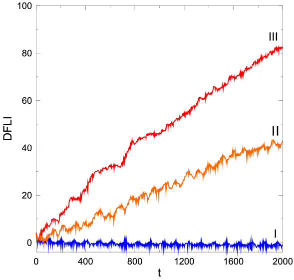
As already stated, the stability of a periodic orbit is defined by the 3 pairs of non unit eigenvalues of the monodromy matrix. However, due to the limited accuracy, we cannot be sure, whether the eigenvalues lie on the unit circle, or not. An estimation of the accuracy of computations can be retrieved by the accuracy of computation of the unit eigenvalues which is about 10 digits. Nevertheless, apart from the linear stability, we estimate the evolution stability by using as index the Fast Lyapunov Indicator (FLI), (Froeschlé et al. 1997) and, particularly, we compute the de-trended FLI, (Voyatzis 2008), defined as
where are deviation vectors (initially orthogonal) computed after numerical integration of the variational equations.
3.1 Examples of periodic orbits
In Fig. 1, we illustrate an 1/2 resonant stable -symmetric periodic orbit111This orbit belongs to the family , see Section 4.2. in the inertial frame and in the projection space of the rotating frame and for planetary masses and . The initial conditions correspond to the planetary orbital elements
Its symmetry is revealed by the projections of the orbit in the planes of the space (see Fig. 1b). The corresponding resonant angles take the values , and .
In Fig. 2, we show an 1/2 resonant -symmetric unstable periodic orbit222This orbit belongs to the family , see Section 4.2.. The planetary masses are and and the initial conditions correspond to the planetary orbital elements
Its symmetry is revealed by the projections of the orbit in the planes of the space (see Fig. 2b). The corresponding resonant angles take the values , and .
The distribution of eigenvalues of the linear stability analysis is presented in Fig. 3. Regarding the stable -symmetric periodic orbit, all eigenvalues lie on the unit circle (Fig. 3a). One pair (of non unit eigenvalues) is very close to 1 and this is shown in the corresponding magnification (Fig. 3c). Concerning the unstable -symmetric orbit there exists one pair of real eigenvalues indicating the instability (Fig. 3b). Also, one pair of eigenvalues is very close to 1 (see the magnification in Fig. 3d).
In Fig.4, we present two different distributions of eigenvalues obtained for two orbits that belong to the family (see Section 4.2). In the first case, we have the presence of complex instability, while in the second one, two pairs of real eigenvalues exist. Along a family of periodic orbits the eigenvalues move smoothly either on the unit circle, or the real axis and can either enter the real axis, or the unit circle. Therefore, the stability type can change along the families. In the rest of the paper, we will indicate whether an orbit is stable or unstable without declaring the particular type of instability.
3.2 Stability of evolution in the vicinity of periodic orbits
It is known, that in the phase space, a stable periodic orbit is surrounded by invariant tori, where the motion is regular and stays in the neighbourhood of the periodic orbit. In the case of an unstable periodic orbit, chaotic domains exist at least close to the periodic orbit. In general, starting from the neigbourhood of an unstable periodic orbit, the evolution of planetary system shows instabilities and chaotic behaviour. Numerical integrations show that such instabilities appear stronger as far as highly eccentric orbits are concerned (Voyatzis 2008). Hereafter, we present some numerical results that show the above mentioned behaviour of orbits.
We consider the initial conditions of the unstable -symmetric periodic orbit given in the previous section (Fig. 2). Since the initial conditions of the periodic orbit are not exact, the instability leads the evolution far from the periodic orbit. In Fig. 5, we present the evolution of the orbital elements , and and the resonant angles , and . We observe that the eccentricity and the inclination of the heavier planet remain almost constant during the whole time of integration. However, the planet after the critical time t.u. destabilizes, its eccentricity increases and then oscillates around a high value. Also, its inclination takes large values and shows large oscillation around , i.e. its motion turns from prograde to retrograde and vice versa. A significant oscillation of the semimajor axis of after t.u. is also, apparent, though the system remains in the mean motion resonance. The resonant angles and initially librate arround , while increases. After the critical time, and start to rotate, while librates irregularly in the domain . The computation of the DFLI (see Fig. 8, case II) shows clearly the chaotic nature of the evolution.
If we start with the initial conditions given for the stable -symmetric periodic orbit (Fig. 1), we will obtain that the orbital elements , , and the resonant angles remain constant for ever (assuming sufficient integration accuracy). Starting near the periodic orbit, and particularly considering a deviation of in (i.e. we set now ), we obtain a regular evolution as it is shown in Fig. 6. The inclination and the eccentricity values of both planets oscillate arround their initial values, while the resonant angles , and show librations around the values which correspond to the periodic orbit, namely , and , respectively. Now, the DFLI does not increase (Fig. 8, case I)
If we start not sufficiently close to the stable periodic orbit, the stability of evolution is not guaranteed. We consider a larger deviation, compared to the deviation used in the previous case. Particularly, we consider a deviation of in and we integrate the orbit. The results are shown in Fig. 7. The chaotic behaviour of the evolution is obvious and finally the planet is scattered. The resonant angles and rotate, but it is remarkable that librates irregularly around . The DFLI clearly shows the chaotic evolution (Fig. 8, case III).
4 Families of periodic orbits
We compute families of periodic orbits for the general spatial problem (3D-GTBP) by analytical continuation of periodic orbits either from the spatial circular restricted problem (3D-CRTBP), called Scheme I, or from the planar general problem (2D-GTBP), called Scheme II. The presentation of such families will be given in projection planes defined by the planetary eccentricity and inclination values.
4.1 Scheme I: Continuation from 3D-CRTBP to 3D-GTBP
We consider the restricted problem with Jupiter moving in a circular planar motion with period and a massless planet which moves in the space. In this problem, we can obtain families of periodic orbits which bifurcate from vertical critical periodic orbits of the planar restricted problem (Hénon 1973). These families exist either when Jupiter is the inner, or the outer planet (resonance either 1/2, or 2/1, respectively).
Following the notation of Kotoulas and Voyatzis (2005), families of periodic orbits which are symmetric with respect to the -plane are denoted by and families of periodic orbits symmetric with respect to the -axis are denoted by . The subscript or indicates the spatial restricted problem (circular or elliptic, respectively) from which these families bifurcate. Moreover, indicates the continuation with respect to the mass of the initially massless body. Also, the corresponding resonance is indicated by a superscript.
We computed and present the families of 2/1 and 1/2 resonant symmetric periodic orbits of the 3D-RTBP in Fig. 9 (see also Hadjidemetriou and Voyatzis (2000) and Kotoulas (2005), respectively). We denote these families by , where the subscript indicates the continuation from plane to space (see Section 4.2). For the 2/1 resonance such families correspond to relatively high eccentricity values of the massless planet . Conversely, in the 1/2 resonance all periodic orbits correspond to almost circular orbits of the massless planet and are unstable.
It is known that the periodic orbits of the 3D-RCTBP of period can be analytically continued, by increasing the planetary mass of the initially massless body to a periodic orbit of the 3D-GTBP of the same symmetry, provided that , where is an integer (Ichtiaroglou and Michalodimitrakis 1980). This is the case for all orbits of the families given in Fig. 9. For the particular computations presented hereafter, we continue analytically the periodic orbits indicated by the dots in Fig. 9 with respect to the mass (inner planet) or (outer planet) according to the resonance 2/1 or 1/2, respectively. These periodic orbits correspond to some initial inclination value of the massless body, or , and identify the generated families.
4.1.1 Families : Continuation from orbits of family with respect to
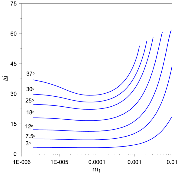
In Fig. 10, we present the continuation of the -symmetric periodic orbits of family . The initial inclination values, , are indicated. The formed families are denoted by and their periodic orbits correspond to the resonant angles
The variation of the eccentricity of the planet along the families with respect to the mass is shown in Fig. 10a. As increases from 0 to (approximately), the eccentricity, , of Jupiter increases rapidly from 0 to 0.25 for all computed families. Then, for small initial inclinations, , of , remains almost constant along the families, but continues to increase for higher initial inclinations, (see panel b). The diagram - (panel c) shows a plateau for the inclination of the inner planet, whose range extends up to almost for the families of small inclination values of . In contrary, Jupiter () shows an almost linear increment of its inclination, as increases (panel d).
Families start having stable periodic orbits. The stability extends up to critical value of , which depends on the particular initial value . In these stable segments the mutual planetary inclination varies, as it is shown in Fig. 11. We observe that we can have stable planetary orbits with mutual inclination, , up to approximately - when the inner planet becomes very massive with respect to Jupiter.
4.1.2 Families : Continuation from orbits of family with respect to
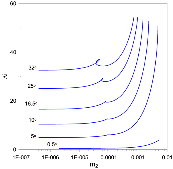
The continuation of the 1/2 resonant -symmetric periodic orbits that belong to the family of the restricted problem is presented (in a similar way as above) in Fig. 12. Since the family is unstable, the families , which are obtained by the analytical continuation with respect to , start having unstable periodic orbits, too. However, as increases the orbits with become stable. Instability becomes again apparent after a larger value of , which depends on the initial inclination, . It is interesting to note that the characteristic curves, which represent the families in the projection planes, show a folding. Namely, for a particular value of we may obtain more than one periodic orbits that belong in the same family. This folding becomes clear in the magnified plot in each panel of Fig. 12. The mutual planetary inclination along the stable segments is shown in Fig. 13. As in the previous case, we obtain stable planetary orbits up to relatively high mutual inclination values (approximately ).
As we have mentioned, the families start with orbits where the eccentricity of the planet is very small. For the corresponding resonant angles of the family of the restricted problem are
For the orbit of changes apsidal orientation and the resonant angles take the values
The orbits of the generated families start with the above resonant angle values, (i) or (ii), accordingly. However, the families that start with the values (i), show a decrement of the eccentricity , as increases. At we obtain a change of the apsidal orientation of and the rest of the family consists of orbits with the resonant angle values (ii).
4.1.3 Families : Continuation from orbits of family with respect to
In Fig. 14, we present the families of -symmetric periodic orbits generated from orbits of the unstable family of the restricted problem. The continuation of these periodic orbits, which is performed by increasing the mass , extends only up to a certain value . Note that the value of for all families is relatively very small (of order ) with respect to Jupiter’s mass . Starting from and by decreasing we can obtain a different branch of the family down to . However, at this point, as far as Jupiter is concerned, we have and , i.e. the families end at periodic orbits of the elliptic restricted problem (3D-ERTBP). Note, now, that Jupiter’s orbit is almost planar in all cases.
All orbits of families are unstable. Their resonant angles are
4.1.4 Families : Continuation from orbits of family with respect to
Similar behaviour as above (start and end) is obtained for the families , where now Jupiter is the inner planet (). All orbits are unstable (Fig. 15).
Concerning the resonant angles, the generating family of the restricted problem starts with orbits having
until . For larger inclination values we have a change in the apsidal orientation and we get the values
The generated families start with the values as above, (i) or (ii) for or , respectively. For case (i), the eccentricity starts decreasing down to zero along the family. Then, the apsidal orientation of planet changes and the resonant angles take the values (ii).
4.2 Scheme II: Continuation from 2D-GTBP to 3D-GTBP
Resonant symmetric periodic orbits for the planar general problem (2D-GTBP) can be obtained by starting from either the circular family of orbits (e.g. Hadjidemetriou (2006a)), or from resonant families of the planar restricted problem (e.g. Antoniadou et al. (2011)). Particularly, for the 2/1 (or 1/2) resonance, planar periodic orbits have been computed by (Beaugé et al. 2006; Voyatzis and Hadjidemetriou 2005; Voyatzis et al. 2009). Now, the distinction between the 2/1 and 1/2 resonance is not essential, since both planetary masses are nonzero and we refer to the mass ratio , where is the inner planet. In the following computations, we always set (Jupiter’s mass). In Fig. 16, we present the 1/2 resonant families and of the general planar problem. The families are given for various values of the mass ratio in the projection space defined by the planetary eccentricities.
The variational equation that corresponds to the -component of the motion of planet is written as333Note that the variational equation given in (Michalodimitrakis 1979a) holds only for the normalization .
| (13) |
where
| (14) |
If , , is the monodromy matrix of Eq. 13 for a planar periodic orbit of period , then, this orbit has a vertical critical index (Michalodimitrakis 1979a) equal to
| (15) |
Any periodic orbit of the planar problem with is vertical critical (v.c.o.) and can be used as a starting orbit for analytical continuation in the spatial problem with the inclination of as a parameter (in computations we increase or ).
In Fig. 16, we present the v.c.o. by dots (see also Tables 1-3). In Fig. 17a, we illustrate the variation of the index along the family for some values of . For , we find three v.c.o. and starting from one of them (see Table 1) we can analytically continue -symmetric periodic orbits in space. We denote such families by where the subscript indicates that the family bifurcates from the general planar problem (it is followed by a number that states the generating planar family) and indicates that the continuation takes place from plane to space. From the remaining couple of v.c.o. (see Table 2) -symmetric periodic orbits in space are obtained forming the families . An example of the above families is given in Fig. 18a in the projection space , where is the mutual inclination. We obtain that the family starts from and ends at v.c.o. of the same planar family . For the couple of v.c.o., from which we obtained the family , disappears. This transition is explained by the variation of the index along the family and is shown in Fig. 17b.
Concerning the families , up to the mass ratio value all the corresponding v.c.o. are unstable and, subsequently, the continuation generates families that start as unstable. The families continue to be unstable until the end of the computations. For the v.c.o. belong to the stable segment of family . Now the generated families start as stable and show a monotonical increase of the inclinations and , and, subsequently, , too (see Fig. 18). The resonant angles that correspond to these periodic orbits are
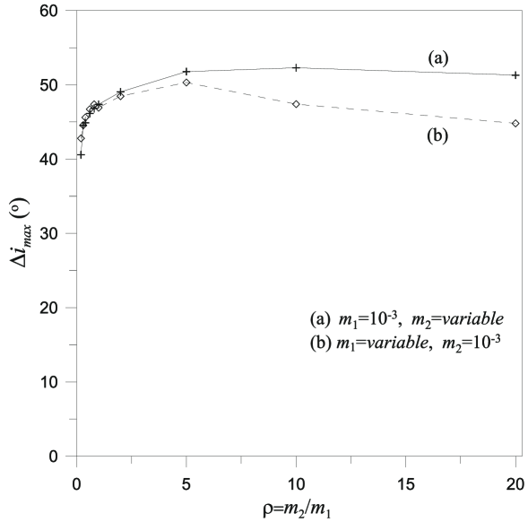
The stability type along the families changes above a maximum value for the mutual inclination, that depends on , as it is shown in Fig. 19. In case (a), Jupiter is the inner planet, , and takes large mass values (up to 20 Jupiter masses), as increases. In case (b), we present the same computations, but now Jupiter is the outer planet, and the other planet, , takes smaller and smaller mass’ values, as increases. We observe that we can have stable orbits up to mutual inclinations and there is no essential difference, whether Jupiter is the inner, or the outer planet in the system.
In Fig. 20, we present the families , which bifurcate from the v.c.o. of families given in Fig. 16b. The corresponding resonant angles are
The families which start from stable v.c.o. (in the range , approximately) show a segment of stable periodic orbits up to a critical mutual inclination value, . seems to increase, as increases in the above mentioned interval and reaches , approximately. The unstable segments show transitions from real to complex instability and vice versa (see e.g. Fig. 4).
5 Miscellaneous cases
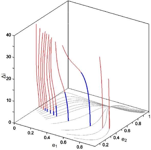
The families are presented in Fig. 10 only for . Further continuation with respect to the mass, , is possible and as a result, we obtain the characteristic curves of Fig. 21a. We observe that for foldings become apparent as in families (see Fig. 12). Also, we can obtain the formation of a loop, given by the separatrix characteristic curve, which includes closed families. Thus, along a family we may obtain more than one periodic orbits (e.g. the periodic orbits A, B and C) that correspond to the same planetary masses.
We have computed the families starting from generating orbits of the 3D-CRTBP. This explains the subscript in their name, although these families end at orbits of the 3D-ERTBP. All of these orbits extend up to a critical mass value, and correspond to inclinations . However, if we consider as starting points periodic orbits of the 3D-ERTBP with then, by continuation with respect to the mass, , we obtain the families which do not end at the circular restricted problem. This is illustrated by the characteristic curves presented in Fig. 21b. We found that a similar situation holds, also, for the 1/2 resonance, namely beside the families (see Fig. 15) there exist, also, families . All of them are unstable.
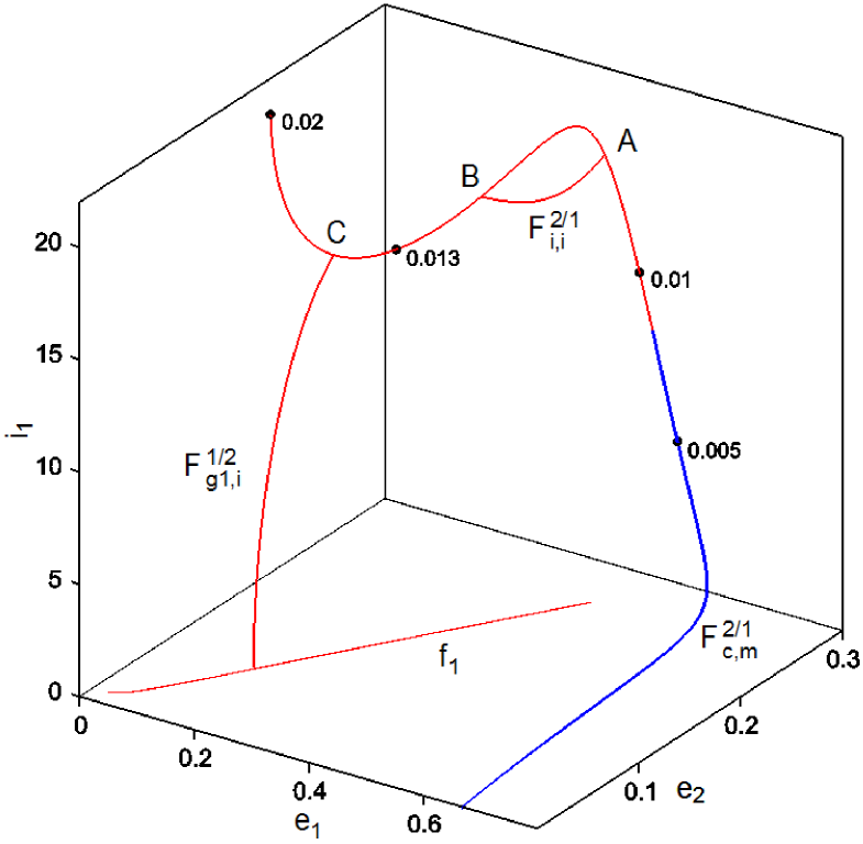
The families obtained by the analytical continuation of Scheme I, consist of periodic orbits with or , namely the planetary orbits are of nonzero inclination. Assuming any of the above mentioned periodic orbits we can apply the continuation of Scheme II, in order to decrease the inclination and terminate in the planar general problem. Then, this terminating point must be a v.c.o. of the planar problem. An example is shown in Fig. 22. We start from the periodic orbit C that belongs to the family for . Along it is (constant). By decreasing , according to the Scheme II, we reach the planar general problem and a v.c.o that belongs to the family with . Thus, we obtain a family. However, this is not always the case. Considering, for example, as a starting periodic orbit, the orbit A, the continuation by varying and keeping constant results to a family that terminates at the orbit B without reaching the plane . This family evolves exclusively in the 3D-GTBP and we denote it by . The existence of a folding (namely two points corresponding to the same planetary masses) is a necessary condition for obtaining such a type of families.
6 Conclusions
In this paper, we presented 2:1 resonant families of periodic orbits in the three dimensional general TBP of planetary type considering a suitable rotating frame of reference, which reduces the system to four degrees of freedom.
Symmetric periodic orbits are of two types: symmetric with respect to the -plane of the rotating frame () and symmetric with respect to the -axis (). For the computation of families of periodic orbits we can apply two continuation schemes:
i) we start from periodic orbits of the 3D circular or elliptic restricted TBP and continue them by varying the mass of the small planet (which is initially the massless body)
ii) we start from vertical critical periodic orbits that belong to the families of the general planar problem and continue them in space by varying the planetary inclination.
The computation and continuation procedures can be applied similarly to any other resonance. Moreover, similar procedures can be used for the computation of asymmetric periodic orbits too, but in this case, it is required to meet a larger number of periodic conditions. Also, we considered and presented orbits only for prograde planetary motion.
Most of the periodic orbits found are linearly unstable. Especially, all periodic orbits symmetric with respect to the of -axis are unstable. In their neigbourhood in phase space, we have planetary orbits that evolve chaotically. We obtain relatively large excitations in eccentricity or inclination and after a relatively short-term evolution the planetary system is disrupted, due to close encounters.
Nevertheless, families of -plane symmetry show segments which include stable periodic orbits. Such orbits can be obtained up to of mutual planetary inclination. Particularly we found that all families which bifurcate from stable vertical orbits of the planar problem start having stable periodic orbits. For the case of the planar family (, ), stability of the bifurcated 3D periodic orbits is observed for a wide range of values of the planetary mass ratio, particularly for and at least up to (where we stopped our computations). For the families of 3D periodic orbits which bifurcate from the planar family (, ) stable orbits exist for . The maximum mutual inclination which is observed for stable orbits increases as increases in the above domain and reaches , approximately. All stable periodic orbits found correspond to quite eccentric planetary orbits (for at least one of the planets).
Starting with initial conditions sufficiently close to a stable periodic orbit the planetary evolution takes place regularly. The planetary system remains in the mean motion resonance and the eccentricities and inclinations show small oscillations. Also, all resonant angles librate around the values that correspond to the stable periodic orbit. Such regions near stable periodic orbits may be considered as strong candidates for hosting planetary systems. The relation between the dynamics of real planetary systems and 3D periodic orbits of the general TBP remains to be studied.
Acknowledgments. We thank Prof. J. Hadjidemetriou and Dr. K. Tsiganis for fruitful discussions about the presented paper. This research has been co-financed by the European Union (European Social Fund - ESF) and Greek national funds through the Operational Program ”Education and Lifelong Learning” of the National Strategic Reference Framework (NSRF) - Research Funding Program: THALES. Investing in knowledge society through the European Social Fund.
References
- Antoniadou et al. (2011) K. I. Antoniadou, G. Voyatzis, and T. Kotoulas. On the bifurcation and continuation of periodic orbits in the three body problem. International Journal of Bifurcation and Chaos, 21:2211, 2011.
- Barnes et al. (2011) R. Barnes, R. Greenberg, T. R. Quinn, B. E. McArthur, and G. F. Benedict. Origin and dynamics of the mutually inclined orbits of andromedae c and d. The Astrophysical Journal, 726:71, 2011.
- Beaugé et al. (2006) C. Beaugé, T. A. Michtchenko, and S. Ferraz-Mello. Planetary migration and extrasolar planets in the 2/1 mean-motion resonance. Monthly Notices of the Royal Astronomical Society, 365:1160–1170, 2006.
- Chatterjee et al. (2008) S. Chatterjee, E. B. Ford, S. Matsumura, and F. A. Rasio. Dynamical outcomes of planet-planet scattering. The Astrophysical Journal, 686:580–602, 2008.
- Correia et al. (2011) A. C. M. Correia, J. Laskar, F. Farago, and G. Boué. Tidal evolution of hierarchical and inclined systems. Celestial Mechanics and Dynamical Astronomy, 111:105–130, 2011.
- Ferraz-Mello et al. (2003) S. Ferraz-Mello, C. Beaugé, and T. A. Michtchenko. Evolution of migrating planet pairs in resonance. Celestial Mechanics and Dynamical Astronomy, 87:99–112, 2003.
- Froeschlé et al. (1997) C. Froeschlé, E. Lega, and R. Gonczi. Fast lyapunov indicators. application to asteroidal motion. Celestial Mechanics and Dynamical Astronomy, 67:41–62, 1997.
- Goździewski et al. (2005) K. Goździewski, M. Konacki, and A. Wolszczan. Long-term stability and dynamical environment of the psr 1257+12 planetary system. The Astrophysical Journal, 619:1084–1097, 2005.
- Hadjidemetriou and Voyatzis (2000) J. Hadjidemetriou and G. Voyatzis. The 2/1 and 3/2 resonant asteroid motion: A symplectic mapping approach. Celestial Mechanics and Dynamical Astronomy, 78:137–150, 2000.
- Hadjidemetriou (2006a) J. D. Hadjidemetriou. Symmetric and asymmetric librations in extrasolar planetary systems: a global view. Celestial Mechanics and Dynamical Astronomy, 95:225–244, 2006a.
- Hadjidemetriou (2006b) J. D. Hadjidemetriou. Periodic orbits in gravitational systems, pages 43–79. Springer Netherlands, 2006b.
- Hadjidemetriou and Voyatzis (2010) J. D. Hadjidemetriou and G. Voyatzis. On the dynamics of extrasolar planetary systems under dissipation: Migration of planets. Celestial Mechanics and Dynamical Astronomy, 107:3–19, 2010.
- Haghighipour et al. (2003) N. Haghighipour, J. Couetdic, F. Varadi, and W. B. Moore. Stable 1:2 resonant periodic orbits in elliptic three-body systems. The Astrophysical Journal, 596:1332–1340, 2003.
- Hénon (1973) M. Hénon. Vertical stability of periodic orbits in the restricted problem. i. equal masses. Astronomy and Astrophysics, 28:415, 1973.
- Ichtiaroglou and Michalodimitrakis (1980) S. Ichtiaroglou and M. Michalodimitrakis. Three-body problem - the existence of families of three-dimensional periodic orbits which bifurcate from planar periodic orbits. Astronomy and Astrophysics, 81:30–32, 1980.
- Katopodis et al. (1980) K. Katopodis, S. Ichtiaroglou, and M. Michalodimitrakis. The family i1v of the three-dimensional general three-body problem. Astronomy and Astrophysics, 90:102–105, 1980.
- Kotoulas (2005) T. A. Kotoulas. The dynamics of the 1:2 resonant motion with neptune in the 3d elliptic restricted three-body problem. Astronomy and Astrophysics, 429:1107–1115, 2005.
- Kotoulas and Voyatzis (2005) T. A. Kotoulas and G. Voyatzis. Three dimensional periodic orbits in exterior mean motion resonances with neptune. Astronomy and Astrophysics, 441:807–814, 2005.
- Laughlin et al. (2002) G. Laughlin, J. Chambers, and D. Fischer. A dynamical analysis of the 47 ursae majoris planetary system. The Astrophysical Journal, 579:455–467, 2002.
- Lee and Peale (2002) M. H. Lee and S. J. Peale. Dynamics and origin of the 2:1 orbital resonances of the gj 876 planets. The Astrophysical Journal, 567:596–609, 2002.
- Lee and Thommes (2009) M. H. Lee and E. W. Thommes. Planetary migration and eccentricity and inclination resonances in extrasolar planetary systems. The Astrophysical Journal, 702:1662–1672, 2009.
- Libert and Tsiganis (2009a) A.-S. Libert and K. Tsiganis. Kozai resonance in extrasolar systems. Astronomy and Astrophysics, 493:677–686, 2009a.
- Libert and Tsiganis (2009b) A.-S. Libert and K. Tsiganis. Trapping in high-order orbital resonances and inclination excitation in extrasolar systems. Monthly Notices of the Royal Astronomical Society, 400:1373–1382, 2009b.
- Marchal (1990) C. Marchal. The three-body problem. Elsevier, Amsterdam, 1990.
- Marzari and Weidenschilling (2002) F. Marzari and S. J. Weidenschilling. Eccentric extrasolar planets: The jumping jupiter model. Icarus, 156:570–579, 2002.
- Michalodimitrakis (1979a) M. Michalodimitrakis. On the continuation of periodic orbits from the planar to the three-dimensional general three-body problem. Celestial Mechanics, 19:263–277, 1979/4/1 1979a.
- Michalodimitrakis (1979b) M. Michalodimitrakis. General three-body problem - families of three-dimensional periodic orbits. ii. Astrophysics and Space Science, 65:459–475, 1979b.
- Michalodimitrakis (1980) M. Michalodimitrakis. General three-body problem - families of three-dimensional periodic orbits. i. Astronomy and Astrophysics, 81:113–120, 1980.
- Michalodimitrakis (1981) M. Michalodimitrakis. The families c 1 v and m 2 v of the three-dimensional general three-body problem. Astronomy and Astrophysics, 93:212–218, 1981.
- Michtchenko and Ferraz-Mello (2011) T. A. Michtchenko and S. Ferraz-Mello. The periodic and chaotic regimes of motion in the exoplanet 2/1 mean-motion resonance. Proceedings of Third La Plata International School on Astronomy and Geophysics: Chaos, diffusion and non-integrability in Hamiltonian Systems Applications to Astonomy, 2011.
- Michtchenko et al. (2006a) T. A. Michtchenko, C. Beaugé, and S. Ferraz-Mello. Stationary orbits in resonant extrasolar planetary systems. Celestial Mechanics and Dynamical Astronomy, 94:411–432, 2006a.
- Michtchenko et al. (2006b) T. A. Michtchenko, S. Ferraz-Mello, and C. Beaugé. Modeling the 3-d secular planetary three-body problem. discussion on the outer andromedae planetary system. Icarus, 181:555–571, 2006b.
- Michtchenko et al. (2008a) T. A. Michtchenko, C. Beaugé, and S. Ferraz-Mello. Dynamic portrait of the planetary 2/1 mean-motion resonance - i. systems with a more massive outer planet. Monthly Notices of the Royal Astronomical Society, 387:747–758, 2008a.
- Michtchenko et al. (2008b) T. A. Michtchenko, C. Beaugé, and S. Ferraz-Mello. Dynamic portrait of the planetary 2/1 mean-motion resonance - ii. systems with a more massive inner planet. Monthly Notices of the Royal Astronomical Society, 391:215–227, 2008b.
- Psychoyos and Hadjidemetriou (2005) D. Psychoyos and J. D. Hadjidemetriou. Dynamics of 2/1 resonant extrasolar systems application to hd82943 and gliese876. Celestial Mechanics and Dynamical Astronomy, 92:135–156, 2005.
- Schwarz et al. (2012) R. Schwarz, Á. Bazso, B. Érdi, and B. Funk. Stability of the lagrangian point in the spatial restricted three-body problem - application to exoplanetary systems. Monthly Notices of the Royal Astronomical Society in press, 2012.
- Thommes and Lissauer (2003) E. W. Thommes and J. J. Lissauer. Resonant inclination excitation of migrating giant planets. The Astrophysical Journal, 597:566–580, November 2003.
- Varadi (1999) F. Varadi. Periodic orbits in the 3:2 orbital resonance and their stability. The Astronomical Journal, 118:2526–2531, 1999.
- Veras and Armitage (2004) D. Veras and P. J. Armitage. The dynamics of two massive planets on inclined orbits. Icarus, 172:349–371, December 2004.
- Voyatzis (2008) G. Voyatzis. Chaos, order, and periodic orbits in 3:1 resonant planetary dynamics. The Astrophysical Journal, 675:802–816, 2008.
- Voyatzis and Hadjidemetriou (2005) G. Voyatzis and J. D. Hadjidemetriou. Symmetric and asymmetric librations in planetary and satellite systems at the 2/1 resonance. Celestial Mechanics and Dynamical Astronomy, 93:263–294, 2005.
- Voyatzis et al. (2009) G. Voyatzis, T. Kotoulas, and J. D. Hadjidemetriou. On the 2/1 resonant planetary dynamics - periodic orbits and dynamical stability. Monthly Notices of the Royal Astronomical Society, 395:2147–2156, 2009.