3-D Rigid Models from Partial Views—
—Global Factorization
Abstract
The so-called factorization methods recover 3-D rigid structure from motion by factorizing an observation matrix that collects 2-D projections of features. These methods became popular due to their robustness—they use a large number of views, which constrains adequately the solution—and computational simplicity—the large number of unknowns is computed through an SVD, avoiding non-linear optimization. However, they require that all the entries of the observation matrix are known. This is unlikely to happen in practice, due to self-occlusion and limited field of view. Also, when processing long videos, regions that become occluded often appear again later. Current factorization methods process these as new regions, leading to less accurate estimates of 3-D structure. In this paper, we propose a global factorization method that infers complete 3-D models directly from the 2-D projections in the entire set of available video frames. Our method decides whether a region that has become visible is a region that was seen before, or a previously unseen region, in a global way, i.e., by seeking the simplest rigid object that describes well the entire set of observations. This global approach increases significantly the accuracy of the estimates of the 3-D shape of the scene and the 3-D motion of the camera. Experiments with artificial and real videos illustrate the good performance of our method.
Index Terms:
3-D rigid structure from motion, complete 3-D models, matrix factorization, factorization with missing data, model selection, penalized likelihood, expectation-maximization, subspace approximation.I Introduction
In areas ranging from virtual reality and digital video to robotics, an increasing number of applications need three-dimensional (3-D) models of real-world objects. Although expensive active sensors, e.g., laser rangefinders, have been frequently used to acquire 3-D data, in many relevant situations only two-dimensional (2-D) video data is available and the 3-D models have to be recovered from their 2-D projections. In this paper, we address the automatic recovery of complete 3-D models from 2-D video sequences.
I-A Related work and motivation
Since the strongest cue to infer 3-D shape from video is the 2-D motion of the image brightness pattern, our problem has been often referred to as structure from motion (SFM). Since using a large number of views, rather than simply two consecutive frames, leads to more constrained problems, thus to more accurate 3-D models, current research has been focused on multi-frame SFM. The factorization method introduced in [38] overcomes the difficulties of multi-frame SFM—nonlinearity and large number of unknowns—by using matrix subspace projections. In [38], the trajectories of feature points are collected into an observation matrix that, due to the rigidity of the 3-D object, is highly rank deficient in a noiseless situation. The 3-D shape of the object and the 3-D motion of the camera are recovered from the rank deficient matrix that best matches the observation matrix. The work of [38] was extended in several ways, e.g., geometric projection models [37, 30], 3-D shape primitives [34, 31, 4], recursive formulation [27], uncertainty [28, 2, 6, 5], multibody scenario [15]. Besides recovering 3-D rigid structure from video sequences, recent approaches to several other image processing/computer vision problems require determining linear or affine low dimensional subspaces from noisy observations. These problems include object recognition [9, 39], applications in photometry [35, 29, 10], and image alignment [42, 43].
In general, such low dimensional subspaces are found by estimating rank deficient matrices from noisy observations of their entries. When the observation matrix is completely known, the solution to this problem is easily obtained from its Singular Value Decomposition (SVD) [16]. However, in practice, the observation matrix may be incomplete, i.e., some of its entries may be unknown (unobserved). When recovering 3-D structure from video, the observation matrix collects 2-D trajectories of projections of feature points [38, 37, 30, 27, 6, 5] or other primitives [34, 31, 28, 4]. In real life video clips, these projections are not visible along the entire image sequence due to the occlusion and the limited field of view. Thus, the observation matrix is in general incomplete. For the specific cases we focus in this paper—videos that show views all around (non-transparent) 3-D objects—this incomplete characteristic of the observation matrix is particularly noticeable.
The problem of estimating a rank deficient matrix from noisy observations of a subset of its entries deserved then the attention of several researchers. References [38] and [24] propose sub-optimal solutions. In [38], the missing values of the observation matrix are “filled in”, in a sequential way, by using SVDs of observed submatrices. In [24], the author proposes a method to combine the constrains that arise from the observed submatrices of the original matrix. More recently, several bidirectional optimization schemes were proposed, e.g., [25, 19, 12, 1, 23, 40, 14], and the problem was also addressed by using nonlinear optimization [13].
However, none of the methods above deal with “self-inclusion”, i.e., with the fact that a region that disappears due to self-occlusion may appear again later. When this happens, the re-appearing region is usually treated as a new region, i.e., as a region that was never seen before. This procedure has two drawbacks: i) the problem becomes less constrained than it should, thus leading to less accurate estimates of 3-D structure; and ii) further 3-D processing is needed to fuse the recovered multiple versions of the same real-world regions.
I-B Proposed approach
We propose a global approach to recover complete 3-D models from video. Global in the sense that our method computes the simplest 3-D rigid object that best matches the entire set of 2-D image projections. This way we avoid having to post-process several partial 3-D models, each obtained from a smaller set of frames, or an inaccurate 3-D model obtained from the entire set of frames without detecting re-appearing regions. We develop a global cost function that balances two terms—model fidelity and complexity penalization. The model fidelity term measures the error between the model—a 3-D shape and a set of re-appearing regions—and the observations, as in Maximum Likelihood (ML) estimation. This error is simply given by the distance of a re-arranged observation matrix to the appropriate space of rank deficient matrices. The penalty term measures the complexity of the 3-D model, which is easily coded by the number of feature points used to describe the observations. By minimizing this global cost, we get what statisticians usually call a Penalized Likelihood (PL) [18] estimate of the 3-D structure. Through PL estimation, re-appearing regions are then detected when the increase of the complexity of the 3-D model does not compensate a slightly better fit to the observations, meaning that a more complex 3-D model would fit the observation noise rather than the 3-D real-world object.
The minimization of the PL cost function requires the computation of rank deficient matrices from partial observations. In the paper, we study two iterative algorithms developed for this problem. The first algorithm is based in a well known method to deal with missing data—the Expectation-Maximization (EM) [26]. Although the authors don’t refer it, the bidirectional scheme in [25] is also EM-based. However, as detailed below, the EM algorithm we propose is more general and computationally simpler than the one in [25]. Our second two-step iterative scheme is similar to Wiberg’s algorithm [41] and related to the one used in [36] to model polyhedral objects. It computes, alternately, in closed form, the row space matrix and the column space matrix whose product is the solution matrix. We call this the Row-Column (RC) algorithm.
In the paper, we illustrate the behavior of both iterative algorithms with simple cases and evaluate their performance with more extensive experiments. In particular, we study the impact of the initialization on the algorithm’s behavior. From these experiments, we conclude that the RC algorithm is more robust than EM in what respects to the sensibility to the initialization. Furthermore, the number of iterations needed for good convergence and the computational cost of each iteration are both smaller for RC than for EM. Obviously, the performances of both EM and RC improve when the initial estimate provided to the algorithms is more accurate. Any sub-optimal method, e.g. the ones in [38, 24], can be used to compute such an initialization. Our experience shows that, with a simple initialization procedure, even for high levels of noise and large amount of missing data, both iterative algorithms converge: i) to the global optimum; and ii) in a very small number of iterations. Naturally, under our global factorization approach, the rank deficient matrices can also be computed by using nonlinear methods such as [13].
We use EM and RC in the context of recovering complete 3-D models from video, through the minimization of our global PL cost. Our experiments show that fitting the rank deficient matrix to the entire (re-arranged) observation matrix (which, naturally, misses several entries) leads to better 3-D reconstructions than those obtained by combining partial 3-D models estimated by fitting submatrices to smaller subsets of data (each corresponding to a subset of features that were visible in a subset of consecutive frames).
I-C Paper organization
In section II we overview the matrix factorization approach to the recovery of 3-D structure. Section III details the problem addressed in this paper—the direct recovery of complete 3-D models from incomplete 2-D trajectories of features points. In section IV we describe our solution as the minimization of a global cost function. Section V describes the algorithms used to estimate rank deficient matrices from incomplete observations. In sections VI and VII, we present experiments and an application to video compression. Section VIII concludes the paper.
II Matrix Factorization for 3-D Structure from Motion
In the original factorization method [38], the authors track feature points over frames and collect their 2-D trajectories in the observation matrix . The observation matrix is written in terms of the parameters that describe the 3-D structure (3-D shape and 3-D motion) as
| (1) |
where and represent the rotational and translational components of the 3-D motion of the camera and represents the 3-D shape of the scene. Matrix is . It collects entries of the 3-D rotation matrices that code the camera orientations. The vector collects the camera positions. Matrix is . It contains the 3-D coordinates of the feature points. See [38] for the details.
The problem of recovering 3-D structure from motion (SFM) is then: given , estimate , , and . Due to the specific structure of the entries of the 3-D rotation matrices in , see for example [7], this is an highly non-linear problem. The factorization method uses a subspace approximation to derive an efficient solution to this problem. In [38], the authors noted that, in a noiseless situation, the observation matrix in (1) belongs to a restricted subspace—the space of the rank 4 matrices. In practice, due to the noise, although the observations matrix is in general full rank, it is well approximated by a rank 4 matrix. The method in [38] recovers SFM performing two separate steps. The first step computes the rank 4 matrix that best matches the observation matrix . The second step performs a normalization that approximates the constraints imposed by the entries of the rotation matrices in .
To compute the rank 4 matrix that best matches the observations, most common techniques use the Singular Value Decomposition (SVD) of . This requires that all entries of are known, which means that the projections of the feature points to be processed were observed in all frames, i.e., that they are seen during the entire video sequence. In real world applications, this assumption limits severely the feature point candidates because very often important regions that are seen in some frames are not seen in others due to the scene self-occlusion and the limited field of view.
III Recovering Complete 3-D Models: Occlusion and Re-appearing Features
Since in many practical situations, several regions of the 3-D scene to reconstruct do not appear in the entire set of images of the video sequence, the observation matrix has several unknown entries. Naturally, a suboptimal solution to the recovery of 3-D structure in such situations is to process separately several completely known submatrices of the observations matrix. However, this leads to a less constrained problem—the global rigidity of the scene is not appropriately modelled.
Another aspect that must be taken into account is the fact that regions that disappear may re-appear later. For example, when attempting to build a complete model of a 3-D object, we must use a video stream containing views that completely “cover” the object, typically, a video obtained by rotating the camera around the object. Obviously, as the camera moves, some feature points disappear, due to object self-occlusion, remain invisible during certain period and then re-appear. In general, each feature point has thus several tracking periods. Although this is always the case when constructing complete 3-D models, it also happens very frequently when processing real-life videos in general.
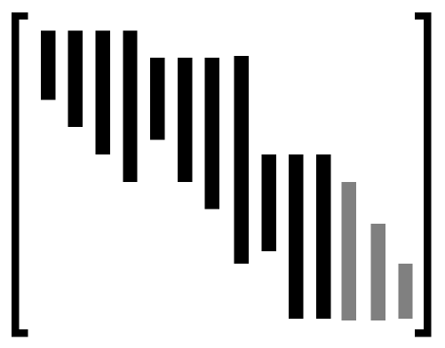
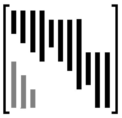
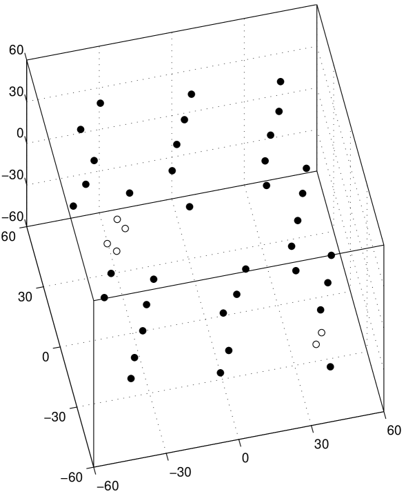
Even current methods that deal with occlusion, e.g., [24, 25, 19, 12, 1, 23, 40, 14, 13], do not consider a re-appearing feature as another observation of a previously seen point. They rather consider as many feature points as tracking periods. To illustrate this point, we represent on the left image of Fig. 1 the typical shape of the known entries of the observation matrix . Each feature trajectory is represented by a column of . The three last columns (in gray) correspond to re-appearing features, i.e., they are second tracking periods of the features that were first tracked and collected in the three first columns. When a given feature has two tracking periods, current methods like the ones in the references above, return a 3-D shape containing two 3-D feature points that correspond to the same 3-D point of the real-world object. Although these two 3-D feature points would coincide in a noiseless situation, in practice they are just close to each other. To demonstrate this, we represent on the left plot of Fig. 2, the 3-D shape recovered from a set of synthesized trajectories of 40 features, by using the method in [19]. To simulate occlusion, three of the trajectories were artificially “interrupted”, leading to three pairs of recovered 3-D points, marked with small circles in the left plot of Fig. 2.
A simple way to detect re-appearing features is based on a local analysis of the distance between recovered 3-D points. However, this procedure is hard in practice due to the sensitivity to the threshold below which the features would be considered to correspond to the same 3-D point. In fact, the distance between the features that correspond to the same 3-D point, depends not only on the noise level but also on the camera-object distance, which is very difficult to estimate accurately enough. The detection of re-appearing features must then be based on a global approach.
Our approach in this paper is then to re-arrange the observation matrix into a smaller matrix that merges all the tracking periods of the same feature in the same column. For the observation matrix shown on the left side of Fig. 1, the re-arranged matrix would be as shown on its right. Finding matrix is equivalent to detecting the re-appearing features. Note that the statements of section II remain valid for the re-arranged matrix ; in particular, is rank 4 in a noiseless situation, just like the original observation matrix . As pointed out before, the advantage of using rather than is that the SFM problem becomes more constrained, thus leading to more accurate estimates of the 3-D structure.
IV Global Approach: Penalized Likelihood Estimation
We formulate the detection of re-appearing features as a model selection problem, where a model is represented by a re-arranged observation matrix . Matrix determines the number of feature points of the 3-D model, , and the correspondences between columns of the original observation matrix and points of the 3-D real-world object. To select the best model , we propose a global approach—we seek the simplest 3-D rigid object that describes the entire set of (incomplete) feature trajectories.
IV-A Penalized likelihood cost
In our approach, re-appearing features are detected through the minimization of a global cost-function that takes into account both the accuracy of the model and its complexity. Thus, the re-arranged matrix is given by
| (2) |
where measures the error of the model as its distance to the space of rank 4 matrices, i.e., it is a likelihood term, and is the number of feature points of the model, i.e., it codes the model complexity (matrix is ). The parameter balances the two terms. Naturally, the minimization in (2) is constrained to the set of matrices that can be found by re-arranging the original observations matrix . We denote this set by .
The likelihood term in (2) models the object rigidity. As outlined in section II, in a noiseless situation, the matrix collecting the trajectories of points of a rigid object is rank 4. This term is then naturally given by the distance of the matrix to the space of the rank 4 matrices. Since not all the entries of are known, we measure this distance by masking the unknown entries:
| (3) |
where represents the Frobenius norm, which arises from assuming that the observations are corrupted by white Gaussian noise, denotes the space of the rank matrices, represents the elementwise product, also known as the Hadamard product, and the matrix is a binary mask that accounts for the known entries of the matrix , i.e., the entry of is if the entry of is known and otherwise.
In Bayesian inference approaches, the term in (2) is considered to be a prior and the minimization (2) leads to the Maximum a Posteriori (MAP) estimate [11] (the cost function in (2) is the negative log posterior probability). Penalization terms, such as in (2), have also been introduced in the model selection literature through information-theoretic criteria like Akaike’s AIC [32] or the Minimum Description Length (MDL) principle [8]. Naturally, different basic principles lead to different choices for the balancing parameter but the structure of the cost function is most often as in (2). This generic form (2) is usually called by the statisticians a penalized likelihood (PL) cost function [18]. In our case, to find a valid range for the weight parameter , we performed several experiences. By testing with pertinent values for the number of features, number of images, noise level, of missing data, and number of re-appearing features, we concluded that there is a wide range of values for that leads to a good balance between maximizing the number of correct detections of re-appearing features (probability of detection) and minimizing the number of incorrect detections (probability of false alarm).
IV-B Minimization algorithm
To find candidates , our algorithm starts by selecting from the original observation matrix , pairs of columns that can be merged with each other. Naturally, these pairs correspond to disjoint tracking periods. For example, for the matrix in the right side of Fig. 1, each one of the six last columns could be merged with the first column, therefore, in what respects to the feature corresponding to the first column, there are seven possible situations: it could either have re-appeared, generating one of the trajectories of the six last columns, or remain occluded for the remaining of the video.
To obtain a computationally feasible algorithm, we prune the search—our algorithm decides by comparing the costs of merging each selected pair of columns with the one of considering that there are not re-appearing features, i.e., of the model . The process is then repeated until the cost (2) does not decrease by merging any selected pair of columns. The search could be further pruned, e.g., using the local approach outlined in the previous section to guide the process, thus testing only pairs of columns corresponding to feature points that are close in 3-D.
What remains to be addressed is the computation of the likelihood term , given by expression (3). The minimization in (3) requires finding the rank 4 matrix that best matches the incompletely known matrix . There is not known closed-form solution for this problem. In the following section, we develop iterative algorithms that compute such rank deficient approximations in very few iterations. The likelihood term is then computed as
| (4) |
where is the rank 4 matrix that best matches the known entries of the matrix , i.e.,
| (5) |
The iterative algorithms we describe in the sequel converge in very few iterations to , when adequately initialized. In the appendix, we describe a strategy to compute such initialization. We reduce the computational burden of the global approach by performing this initialization step only once, when testing the model that corresponds to the original observation matrix, , and using the same initial guess when testing the other models.
V Estimation of rank deficient matrices with Missing Data
We now address the estimation of the rank deficient matrix given by expression (5). To gain insight and introduce notation, let us first consider the case where the matrix is completely known, i.e., . In this case, (5) is simplified to
| (6) |
The solution of (6) is known—it is obtained by selecting the largest singular values, and the associated singular vectors, from the Singular Value Decomposition (SVD), , of the matrix [16]. We denote this optimal rank reduction, i.e., the projection onto , by :
| (7) |
When matrix misses a subset of its entries, the estimation of leads to the minimization of (5), a generalized version of (6). The existence of unknown entries in prevents us to use the SVD of as in (7). In the following subsections we introduce two iterative algorithms that minimize (5). Both algorithms are initialized with a guess , computed as described in the appendix.
V-A Expectation-Maximization algorithm
The Expectation-Maximization (EM) approach to estimation problems with missing data works by enlarging the set of parameters to estimate—the data that is missing is jointly estimated with the other parameters. The joint estimation is performed, iteratively, in two alternate steps: i) the E-step estimates the missing data given the previous estimate of the other parameters; ii) the M-step estimates the other parameters given the previous estimate of the missing data, see [26] for a review on the EM algorithm.
In our case, given the initial estimate , the EM algorithm estimates in alternate steps: i) the missing entries of the input matrix ; ii) the rank matrix that best matches the “complete” data. The algorithm performs these two steps until convergence, i.e., until the error measured by the Frobenius norm in (5) stabilizes.
V-A1 E-step—estimation of the missing data
Given the previous estimate , the estimates of the missing entries of are simply the corresponding entries of . We then build a complete observation matrix , whose entry equals the corresponding entry of the matrix if was observed or its estimate if is unknown,
| (8) |
or, in matrix notation,
| (9) |
V-A2 M-step—estimation of the rank deficient matrix
We are now given the complete data matrix , with the estimates of the missing data from the E-step. The rank matrix that best matches in the Frobenius norm sense, is then obtained from the SVD of , as in (7),
| (10) |
In reference [25], the authors develop a bidirectional algorithm to factor out an observation matrix with missing data, in the context of recovering rigid SFM. Their bidirectional algorithm is in fact an EM algorithm developed to the specific strategy of treating the 3-D translation separately. In opposition, the EM algorithm just described is general, i.e, it solves any rank deficient matrix approximation problem with missing data. Furthermore, our E-step in (9) is simpler than the corresponding step of [25] that requires inverting matrices.
V-B Row-Column Algorithm
We now describe the Row-Column (RC) algorithm—another iterative approach, similar to Wiberg’s algorithm [41], to the estimation of a rank deficient matrix that best matches an incomplete observation. From our experience, summarized in section VI, the RC algorithm is not only computationally cheaper than EM, avoiding SVD computations and exhibiting faster convergence, but also more robust than EM to initializations far from the solution.
For the RC algorithm, we parameterize the rank matrix in (5) as the product
| (11) |
where determines the column space of and its row space. The rank 4 matrix that best matches is obtained by minimizing the cost function in (5) with respect to (wrt) the column space and row space matrices, i.e.,
| (12) |
By using the re-parameterization (11), we map the constrained minimization (5) wrt into the unconstrained minimization (12) wrt and .
We minimize (12) in two alternate steps: i) the R-step assumes the column space matrix is known and estimates the row space matrix ; ii) the C-step estimates for known . The algorithm is initialized by computing from the initial estimate and it runs until the value of the norm in (12) stabilizes.
When there is no missing data, i.e., when in (12), the R- and C- steps above are linear least squares (LS) problems whose solutions are obtained by using the Moore-Penrose pseudoinverse [16],
| (13) |
If we write steps R and C together as a recursion on one of the matrices or , say, on the column space matrix , we get
| (14) |
which shows that, in the no missing data case, our RC algorithm is in fact implementing the application of the power method [16] to the matrix (the factor is the normalization). The power method has been widely used to avoid the computation of the entire SVD when fitting rank deficient matrices to complete observations. We will see that, even when there is missing data, both R- and C- steps admit closed-form solution and the overall algorithm generalizes the power method in a very simple way.
V-B1 R-step—estimation of the row space
For known , the minimization of (12) wrt can be rewritten in terms of each of the columns of ,
| (15) |
where and denote the columns of and , respectively. Exploiting the structure of the binary column vector , we now re-arrange the minimization in (15) in such a way that its solution becomes obvious. First, we note that in (15) is just selecting the entries of the error vector that affect the error norm. Then, by making explicit that selection in terms of the entries of that contain known data and the corresponding relevant entries of , we rewrite (15) as
| (16) |
Note that in (16) is simply a matrix with all columns equal to .
The minimization in (16) is now clearly expressed as a linear LS problem. Its solution is then obtained by using the pseudoinverse of matrix ,
| (17) |
which is simplified by omitting repeated binary maskings,
| (18) |
The set of estimates as in (18) generalizes the well known pseudoinverse LS solution in (13) to problems with missing data.
V-B2 C-step—estimation of the column space
Given , the estimate of each row of the column space matrix is obtained by proceeding in a similar way as in the R-step. We get, for each ,
| (19) |
where in this case, for commodity, lowercase boldface letters denote rows rather than columns.
VI Experiments—rank reduction with missing data
Since approximating rank deficient matrices from incomplete observations is a key step in recovering 3-D structure, we start by describing experiments that illustrate the behavior of the EM and RC algorithms just described and demonstrate their good performance.
VI-A 22 matrices
We start by a simple case that allows an illustrative graphical representation—approximating rank 1 matrices from observations that miss one of the entries. In this case, the error measured by the Frobenius norm in expressions (4) and (12), can be expressed in terms of a single parameter . In fact, let the rank 1 matrix be written in terms of its column and row spaces as in (11),
| (20) |
Without loss of generality, impose that the row vector has unit norm and write it in terms of a row angle ,
| (21) |
Now denote the minimum of (12) wrt the column space for fixed row space , i.e., for fixed , by , given by (19). The error in (4) and (12) is then rewritten as a function of as
| (22) |
Note that for any set of three entries of a matrix, there is always a value for the forth entry that makes the rank of the matrix equal to one, i.e., there is always a rank 1 matrix that fits exactly the observed entries of . Thus, we have .
The examples in the sequel illustrate the impact of the initialization on the behavior of the EM and RC algorithms with experiments that use the following ground truth rank 1 matrix , observation mask , and observation :
| (23) |
where “” represents the unobserved entry of the observation matrix .
VI-B Typical good behavior of EM and RC
Using the initial guess
| (24) |
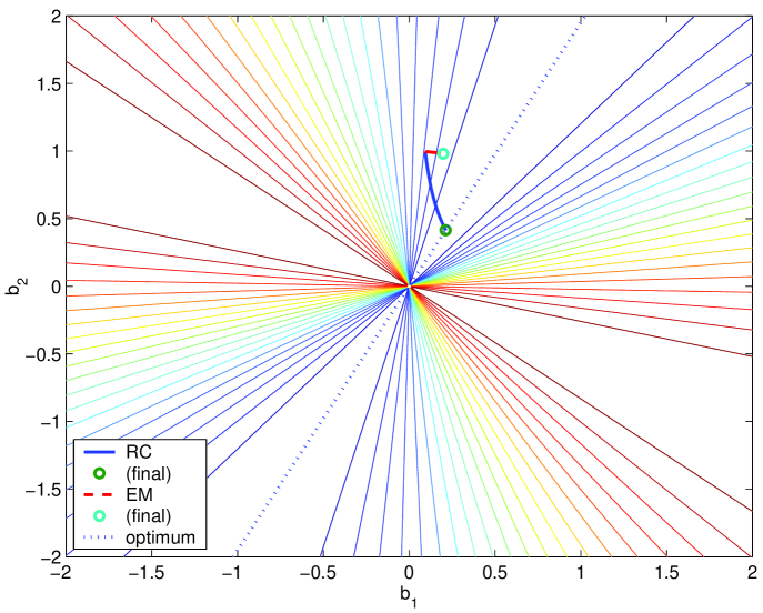
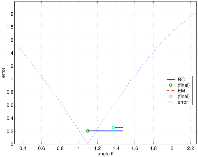
we describe the evolution of the estimates of the rank 1 matrix by plotting two equivalent representations of : i) its row space ; and ii) the corresponding angle as defined in (21). The left plot of Fig. 3 shows the level curves of the error function as function of the row vector , superimposed with the evolution of the estimates of for EM (dashed line) and RC (solid line). In this plot, the dotted line (optimum) are the row vectors that lead to zero estimation error. The right plot of Fig. 3 represents the same error function, now as a function of , as defined in (22), (dotted line) superimposed with the locations of the estimates for EM (dashed line) and RC (solid line).
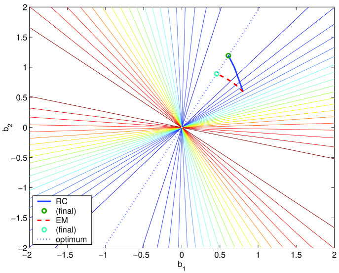
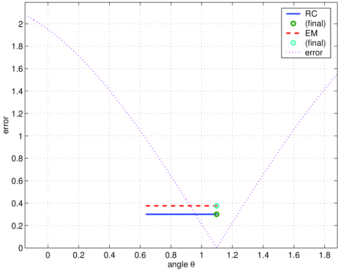
From the left plot of Fig. 3, we see that both EM and RC trajectories start at the same point (due to the equal initialization) and converge to points in the optimal line. As expected, the EM estimates of the row space vector have constant unit norm (due to the normalization in the SVD) while the RC estimates don’t. The good behavior of the algorithms is confirmed by the right plot of Fig. 3 that shows that both algorithms converge to a value of that makes , i.e., that minimizes .
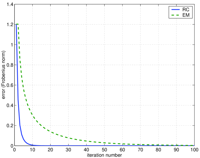
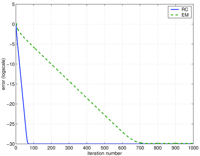
To evaluate the convergence speed, we show in Fig. 4 the evolution of the estimation error along the iterative process for both algorithms (in the left plot, linear scale, in the right one, logarithmic scale). From Fig. 4, we see that RC converges in a smaller number of iterations than EM. Our experience with larger matrices in practical applications have confirmed the faster convergence of RC.
VI-C Large entries in rows or columns that miss data
We now illustrate a drawback of the EM algorithm. Using the same data and the initial estimate
| (25) |
we get the first iterations of Fig. 5, which is as described above for Fig. 3.
From the left plot of Fig. 5, we see that, while RC converges to the optimal line, the estimates given by the EM almost don’t change along the iterative process. This can also be seen in the right plot of Fig. 5, which shows that RC converges to the such that , while EM, after iterations is still far from . The left plot of Fig. 6 shows the evolution of the estimation errors. See that while the error of RC converges to zero in a few iterations, the error of EM almost doesn’t decrease during the first iterations.
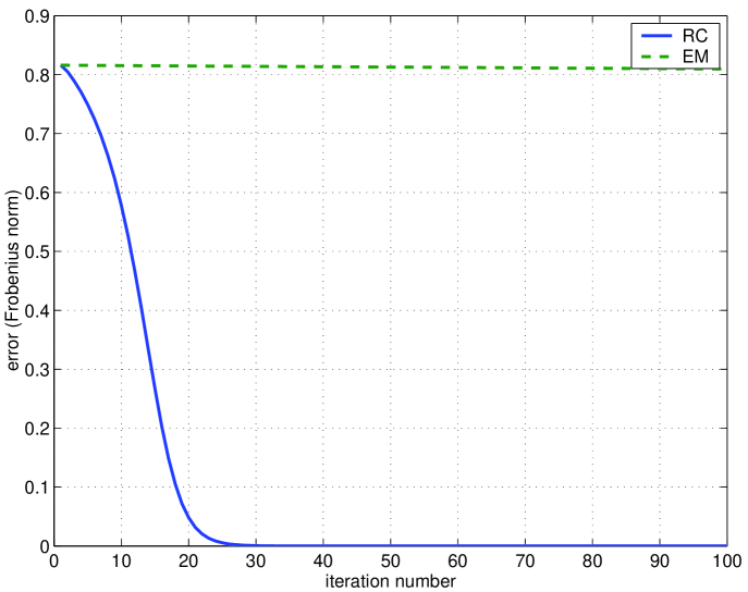
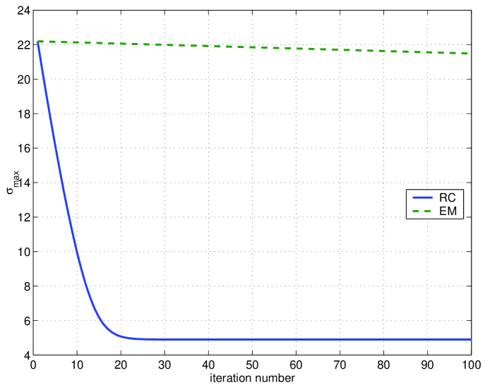
The bad behavior of EM is due to the large initial guess for (note that is large when compared with the known entries of ). Remember that EM starts by estimating the rank 1 matrix that best matches the initial guess . This rank 1 matrix is the matrix associated with the largest singular value of , which is highly constrained by the large spurious entry (note that while the singular values of the ground truth matrix are and , the singular values of the initial guess are and due to the large entry ). Then, EM replaces the known entries of in the new estimate (obtaining thus an estimate that is very close to the initial guess) and repeats the process. To better illustrate this very slow convergence of EM, we represent, in the right plot of Fig. 6, the evolution of the largest singular value of the estimate for both algorithms. We see that while, as expected, the largest singular value of the RC estimates converges to the largest singular value of the solution , , the largest singular value of the first iterations of the EM estimates changes very slowly from its initial value .
The behavior just described also happens in situations other than the initial guesses of the unknown entries being too large when compared to the other entries. In fact, we observed the same behavior in situations where the observation matrix had large entries in rows or columns that contained missing entries. In these situations, due to those large entries, even small values for initial guess of the unknown entries had large impact on the row and column singular vectors associated with the large singular values that determined the best rank deficient approximations to the complete data matrices involved in EM. This lead to the same kind of very slow convergence illustrated in Fig. 5 and Fig. 6.
VI-D Large matrices
We now present results of approximating matrices likely to appear when processing real video sequences. We tested the EM and RC algorithms with noisy partial observations of rank 4 matrices. We used matrices with dimensions ranging from to . The percentage of missing entries ranged from to . We studied the behavior of the EM and RC algorithms in terms of the observation noise power and the amount of missing data, and the impact of the initialization.
We initialized both EM and RC with random values for the unknown entries. To illustrate the influence of the initialization on the convergence of the algorithms, Fig. 7 shows the percentage of experiments that converged (to an estimate close enough to the ground truth) in less than 100 iterations, as a function of the mean value of the random guesses for the unknown entries. Although representative for the entire range of experiments done, the results in the plots of Fig. 7 were obtained with noisy observations of rank 4 matrices that missed of their entries. The left plot of Fig. 7 shows three lines, each obtained by using EM with data generated with a ground truth matrix whose elements had mean , , and . The percentages of convergence for the RC algorithm are in the right plot.
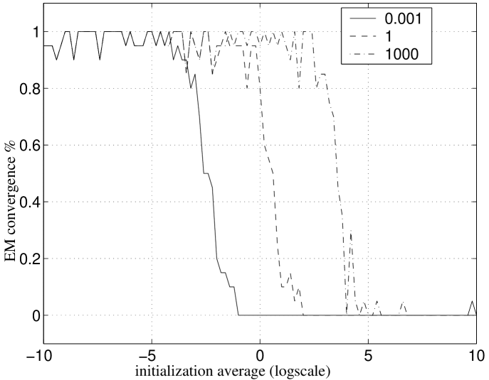
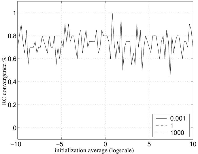
The left plot of Fig. 7 shows that the EM algorithm converges almost always if the mean value of the initial guesses for the missing entries is smaller than the mean value of the observed entries. When we increase the values of the initial estimates of the missing entries, the percentage of convergence decreases abruptly, becoming close to zero when those values become much larger than the ones of the observed entries. This is in agreement with the behavior illustrated in the example of Fig. 5. In opposition, the right plot of Fig. 7 shows that the behavior of the RC algorithm is somewhat independent of the order of magnitude of the initialization. The experiments that lead to a non-convergent behavior of RC were such that the matrices whose inverse is computed in (19) and (18) were close to singular. We thus conclude that it is very important in practical applications to provide good initial estimates for both EM and RC algorithms.
Finally, we note that the relevance of a good initialization goes behind avoiding non-convergent behavior. In fact, we observed that both the amount of missing data and the noise level have strong impact on the algorithm’s convergence speed. Thus, when dealing with large percentages of missing entries and high levels of noise, as it may arise in practice, a better initialization not only improves the chance of a convergent behavior but also leads to a faster convergence.
VI-E Heuristic initialization
We now use an initial guess obtained by combining the column and row spaces given by the SVDs of the known submatrices of as described in the appendix. In our tests, with this simple initialization procedure, of the runs of EM and RC converged to the ground truth matrix (mean square estimation error smaller than the observation noise variance) in a very small number of iterations, typically less than 10, even for high levels of noise.
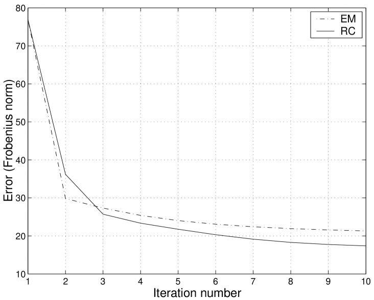
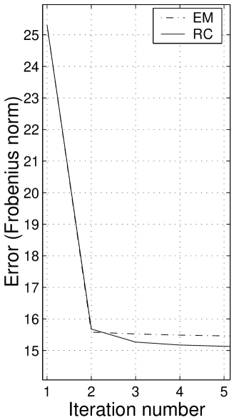
To illustrate the impact of a better initialization, we use a noisy observation of a rank deficient matrix with missing entries (observation noise variance ). Figure 8 shows plots of the evolution of the estimation error, measured by the Frobenius norm, for both the EM and RC algorithms. While for the left hand side plot we used a random initialization, for the one in the right we used the complete procedure, i.e., we initialized the process by using the method described in the appendix. Since the error for the ground truth matrix is given by , we see from the plots of figure 8 that both the EM and RC algorithms provide good estimates. From the right hand side plot, we conclude that the initial guess provided by the heuristic method in the appendix enables a much faster convergence (in 2 or 3 iterations) to a solution with lower error.
VI-F Sensitivity to the noise
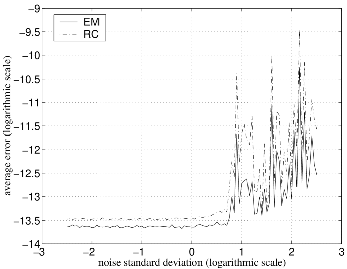
The plot of Fig. 9 represents the average estimation error per entry after 20 iterations of EM and RC algorithms, for noisy observations of a rank 4 matrix , with missing data, as a function of the observation noise standard deviation. We see that the average entry estimation errors after iterations are below for noise standard deviation ranging from to (the mean value of the entries of the ground truth matrix is ). This shows that, with a simple initialization procedure, both EM and RC algorithms converge to the optimal solution, even for very noisy observations. Furthermore, we conclude that the main impact of the observation noise is on the EM and RC convergence speeds—the slightly higher average error values on the right region of the plot of Fig. 9 indicates that the estimates were still converging to the optimal solution after iterations.
VI-G Sensitivity to the missing data
A relevant issue is the robustness of the rank reduction algorithms to the missing data. Our experience showed that the structure of the binary mask matrix representing the known data is more important than the overall percentage of missing entries of . When recovering 3D structure from video, feature points enter and leave the scene in a continuous way, thus the typical structure of is as represented in the left plot of Fig. 1, or, when considering re-appearing features, as represented in the right plot of the same Figure. We tested the EM and RC algorithms with several mask matrices with this typical structure, with the heuristic initial guess. In these experiments, the algorithms converged always to the optimal solution in a very small number of iterations, independently of the percentage of missing data.
Similarly to the impact of the noise discussed above, the percentage of missing entries has impact on the convergence speed. In fact, we concluded that the larger is the portion of the matrix that is observed, i.e., the smaller is the percentage of missing data, the lower is the estimation error after a fixed number of iterations, i.e., the faster is the convergence of the iterative algorithms.
VI-H Computational cost
As referred above, the EM and RC algorithms converge in a very small number of iterations when initialized by the heuristic procedure described in the appendix. We now report an experimental evaluation of the computational costs of each iteration of EM and RC as functions of the observation matrix dimension.
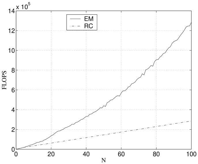
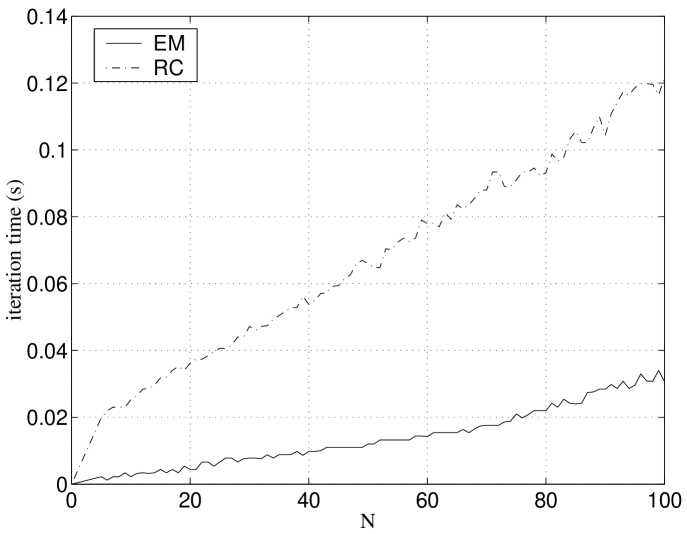
We used observation matrices with missing data corresponding to a submatrix. The plots in Fig. 10 represent the number of MatLab© floating point operations (FLOPS) and the computation time per iteration, as functions of . From the left plot, we see that the number of FLOPS per iteration of the EM algorithm is larger than one of the RC algorithm. Furthermore, the FLOPS count for EM increases exponentially with (due to the SVD computation) while for RC it increases linearly with . Thus, although the computation times in the right plot of Fig. 10 are smaller for EM than for RC (the reason being the very efficient MatLab© implementation of the SVD), we conclude that RC is computationally simpler than EM. RC is even as simple as the methods to deal with complete matrices, since the most efficient way to compute the SVD is to use the power method [16] of which RC is a simple generalization.
VII Experiments—3-D models from video
We now describe experiments that illustrate our method to recover 3-D rigid shape and 3-D motion from video. Our results show: i) how the iterative algorithms of section V cope with video sequences with occlusion; and ii) how the global method we propose recovers complete 3-D models. The experiments use both synthesized and real video sequences. We also describe an application of the recovered 3-D models to video compression.
VII-A Self-occlusion—ping-pong ball video sequence
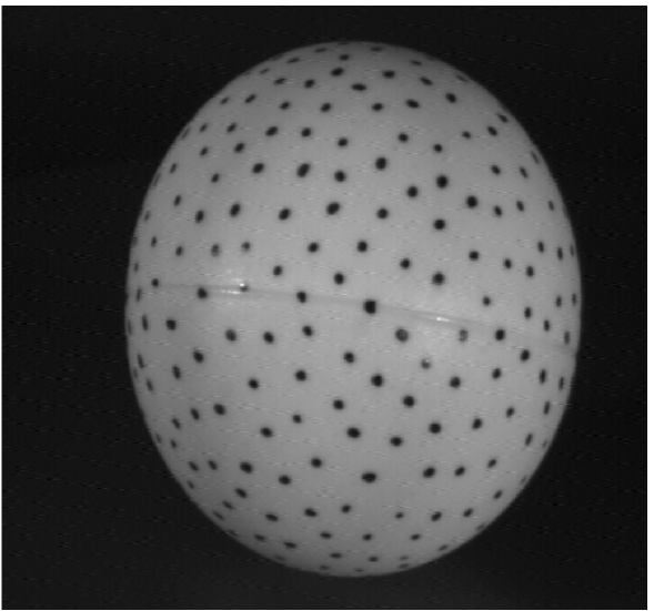
We used a real-life video clip available at [22]. This clip shows a rotating ping-pong ball with painted dots. The left image of Fig. 11 shows the first of the video frames of the ball sequence. Due to the rotating motion, the ball occludes itself. However, it does not complete a turn, thus there are not re-appearing regions.
We used simple correlation techniques to track a set of feature points (these techniques are adequate for the short baseline video sequences we used but more sophisticated methods to cope with wide baselines are available in the literature [33]). Due to the camera-ball 3D rotation, the region of the ball that is visible changes along time, leading to an observation matrix with missing entries. We used the RC algorithm to estimate the rank 4 matrix that best matched the observation and computed the 3-D structure by proceeding as in the factorization method of [38].
In the right image of Fig. 11, we represent the recovered 3-D shape, which shows that our method succeeded in recovering the spherical surface of the ball.
VII-B Complete 3-D models
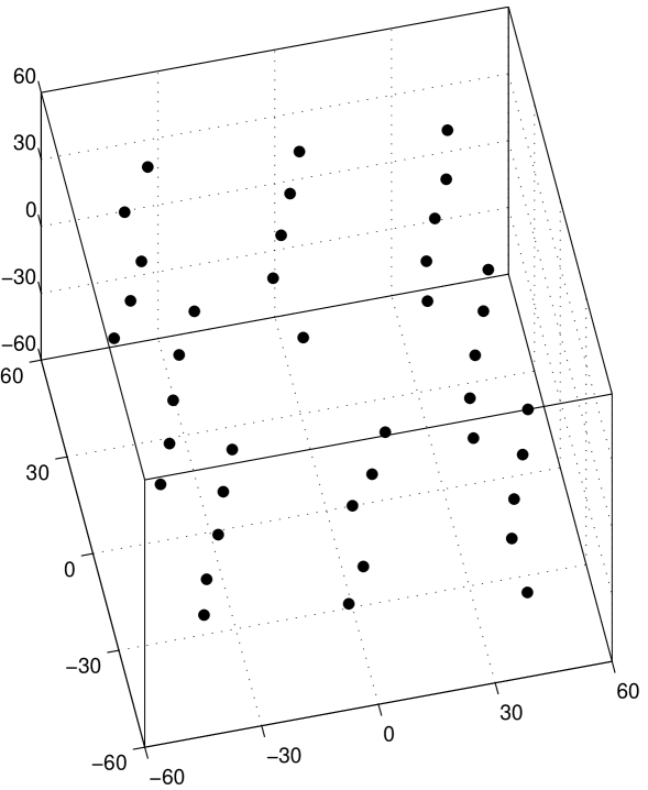
We now illustrate our method to recover complete 3-D models from video by minimizing a global cost function as described in section IV. We processed the observation matrix that lead to the left plot of Fig. 2. The 3-D shape recovered by our global method is shown in the right plot, where each of the pairs of re-appearing features have been correctly detected as representing the same 3-D point.
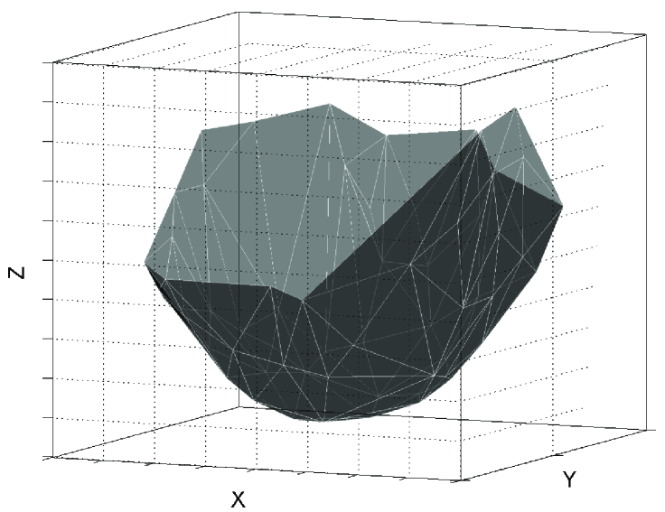
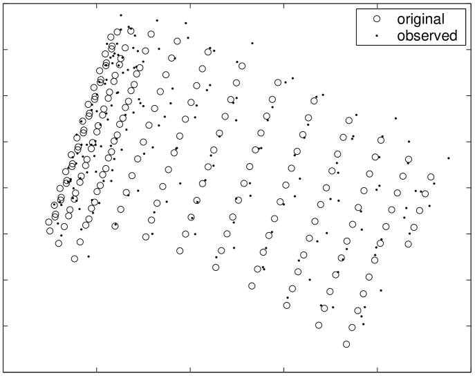
Fig. 12 describes an experiment with an object described by a larger number of 3-D feature points. We synthesized noisy versions of the 2-D trajectories of feature points located on the 3-D surface of a rotating cylinder. Then, we simulated occlusion and inclusion by removing significant segments of those trajectories. The left plot of Fig. 12 shows one of the synthesized frames. The small circles denote the noiseless projections and the points denote their noisy version, i.e., the data that is observed. Note that only an incomplete view portion of the cylinder is observed in each frame.
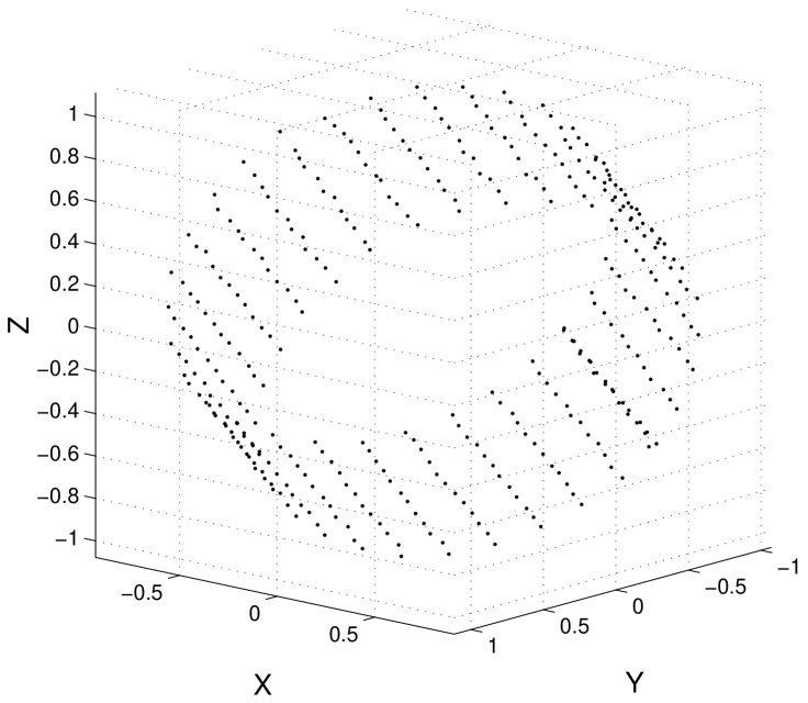
The data from the cylinder sequence was then collected on a observation matrix with 9537 unknown entries ( of the total number). We used the global factorization algorithm to find the re-arranged matrix , i.e., to recover simplest 3-D rigid structure that could have generated the data. The right plot of Fig. 12 plots the final estimate of the 3D shape. We see that the complete cylinder is recovered. Due to the incorporation of the rigidity constraint, the 3D positions of the features points are accurately estimated, even in the presence of very noisy observations (compare the plots in Fig. 12).
VII-C Error analysis
We quantified the gain of using our method to recover SFM by measuring the 3-D reconstruction error. We synthesized noisy trajectories of 40 features randomly located in 3-D, 15 of them being “interrupted” to simulate object self-occlusion, leading to a observation matrix with 53.9% known entries ( and coordinates in , noise standard deviation ). Our method generated a re-arranged matrix with 74.2% known entries. By using rather then to recover SFM, we reduced the 3-D shape estimation error by approximately 50% and the 3-D motion error by approximately 70%.
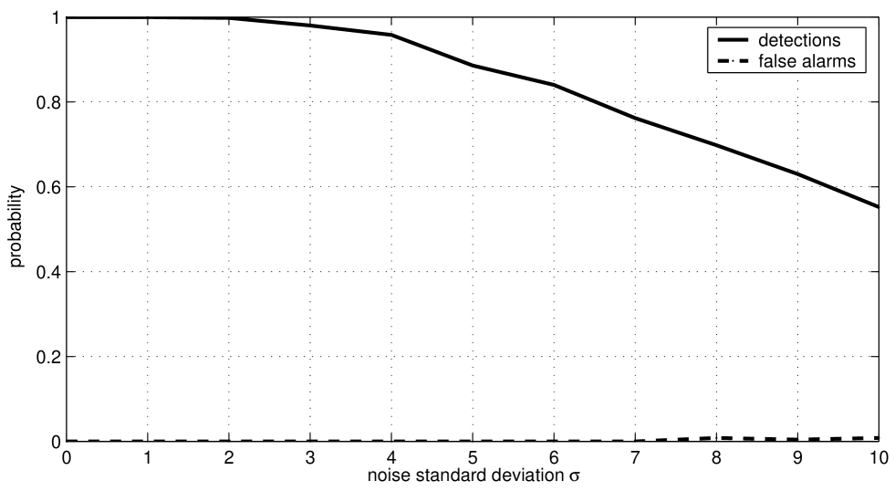
In order to evaluate the sensitivity of our method to the observation noise, we plotted in Fig. 13 the probabilities of correctly detecting re-appearing features and the probability of incorrect detections (false alarms) as functions of the noise level, for the experimental setup described above. These probabilities were estimated from 100 runs for each level of noise. Although re-appearing features become harder to detect as the noise level increases, our method correctly detects more than 90% of them when the noise level is below . The plot of Fig. 13 also shows that our method has approximately zero false alarms for noise levels below . Note that the and coordinates are in , so this level of performance seems to indicate that our method is able to cope with the noise in trajectories likely to happen when processing the majority of real videos.
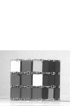
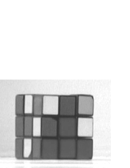
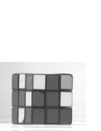
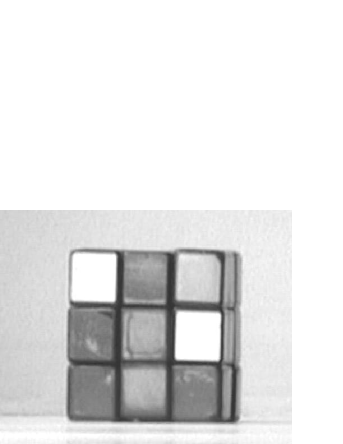
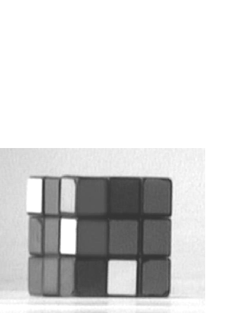
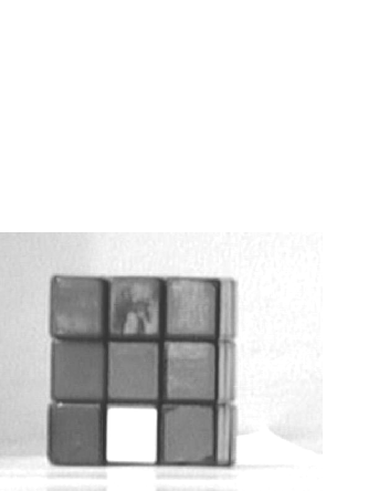
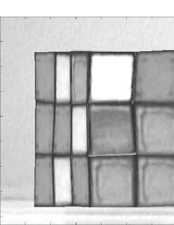
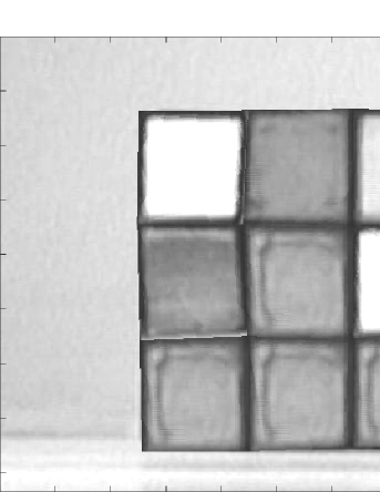
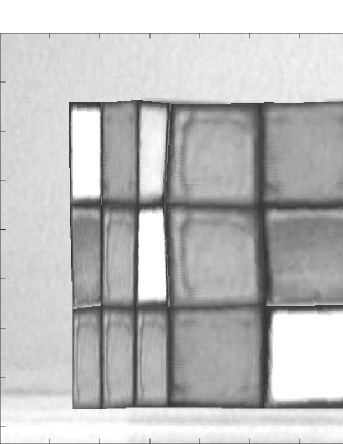
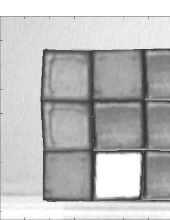
VII-D Real video—Rubik’s cube
This video—see two representative frames on the left and middle images of Fig. 14—shows a Rubik’s cube. The video sequence was obtained by rotating a hand-held camera around a table with the cube. In the leftmost image of Fig. 14, we superimposed with the video frame the visible features and the initial parts of their trajectories. Due to the cube self-occlusion, feature points enter and leave the scene. In particular, along the video sequence, all features disappear and several of them re-appear because the camera performs a complete turn around the cube.
To emphasize the advantages of using the algorithms described in this paper, we first applied to a segment of the Rubik’s cube video clip the original factorization method of [38] for complete matrices, obtaining the 3D shape represented on the left side of Fig. 15. This model was obtained with features and frames.
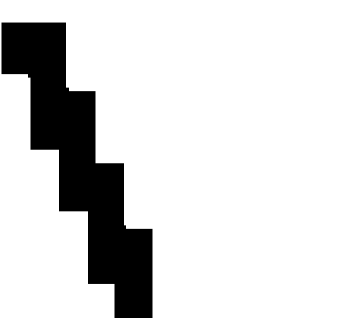
We then collected the entire set of the visible parts of the trajectories of features across frames in a incomplete observation matrix . The structure of the missing part of is coded by the binary mask represented on the right side of Figure 14. The number of missing entries in was about . We computed the re-arranged matrix by using our global factorization. The right image of Fig. 15 shows the texture-mapped 3-D shape recovered from .
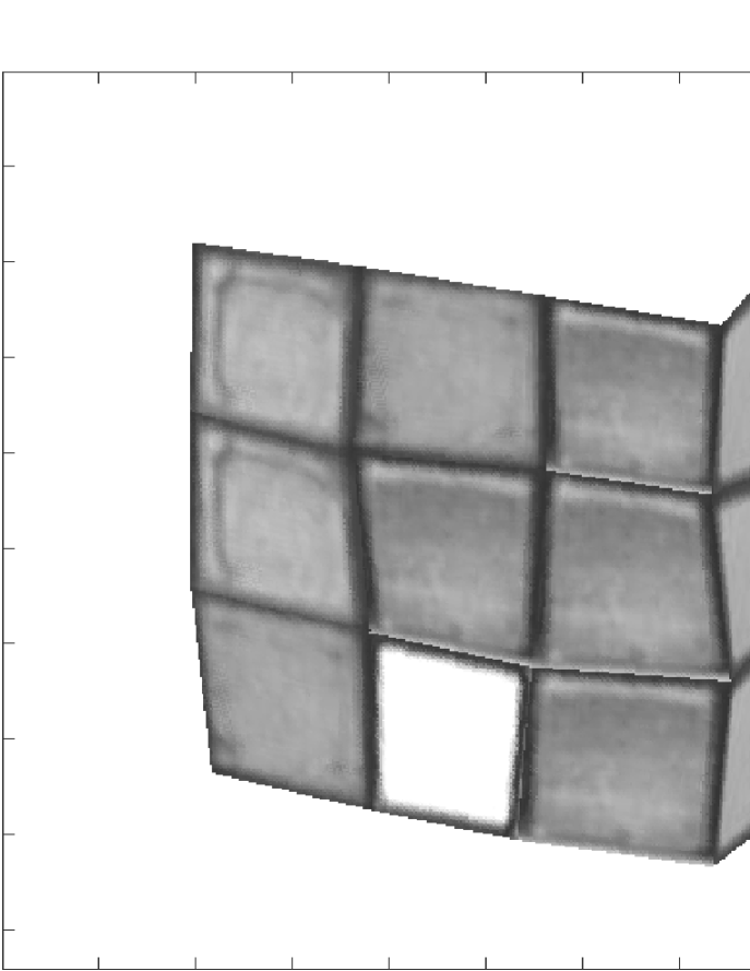
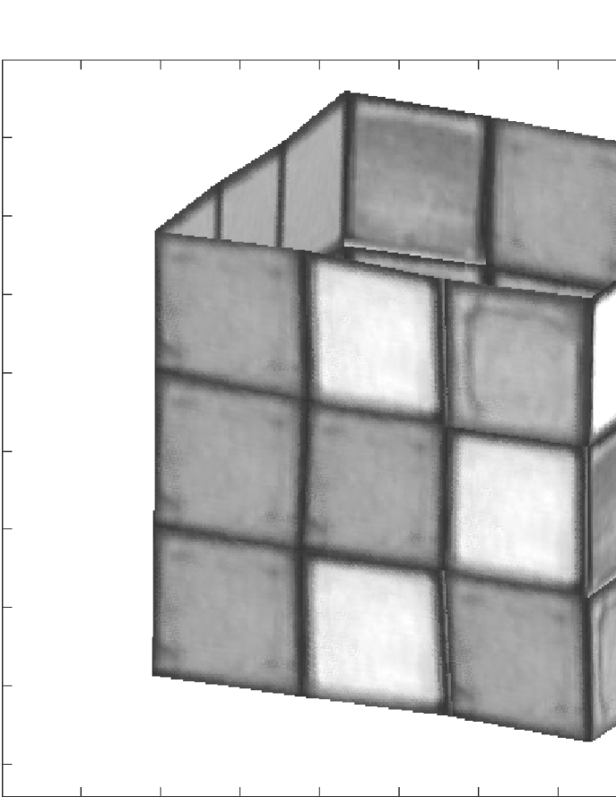
This example illustrates how our global approach trivializes the usually hard task of merging partial estimates of a 3D model like the one in the left image of Fig. 15. Note that the top face is missing also in the right image of Fig. 15 because the position the cube model is shown in that image was not seen in the video sequence. The advantage of using our approach to recover 3-D rigid structure is two-fold. First, while recovering a complete 3-D model by fusing partial models as the one on the left side of Fig. 15 is a complex task, our method recovers directly the complete model shown on the right side of Fig. 15. Second, rather than processing subsets of the set of features and frames at disjoint steps, our method uses all the information available in a global way, leading to more accurate 3-D shapes as illustrated by the 3-D models in Fig. 15.
VII-E Video compression
The 3D models recovered by our method can be used to represent in an efficient way the original video sequence as proposed in [3]—the video sequence is represented by the 3-D shape, texture, and 3-D motion of the objects. This leads to significant bandwidth saving since once the 3-D shape and texture of the objects have been transmitted, their 3-D motion is transmitted with a few bytes per frame.
We used this methodology to compress the entire sequence of frames of the Rubik’s cube video clip. The compression ratio (relative to the original J-PEG compressed frames) was approximately . Fig. 16 shows sample original frames (top row) and the corresponding compressed frames (bottom row). The differences of lighting between the top and bottom images are due to fact that the constancy of the texture of the 3-D model does not model the different light reflections that happen in the real scenario.
VIII Conclusion
We proposed a global approach to build complete 3-D models from video. The 3-D model is inferred as the simplest rigid object that agrees with all the observed data, i.e., with the entire set of video frames. Since a key step in this global approach is the approximation of rank deficient matrices from incomplete observations, we developed two iterative algorithms to solve this non-linear problem: Expectation-Maximization (EM) and Row-Column (RC). Our experiments showed that both algorithms converged to the correct estimate whenever initialized by a simple procedure and that the RC algorithm is computationally cheaper and more robust than EM. Our experiments show that the proposed global method leads to more accurate estimates of 3-D shape than those obtained by either processing several smaller subsets of views or processing the entire video without taking into account re-appearing regions.
This appendix addresses the computation of a rank 4 initial guess from an incomplete observation . We find by computing, in an expedite way, guesses of its column space matrix and its row space matrix , from the data in :
| (26) |
-A Subspace approximation
Before addressing the general case, we consider the simpler case where a number of columns of are entirely known, i.e., a number of feature points are present in all frames, and a number of rows of are entirely known, i.e., and a number of frames contain all feature projections. We collect those known columns in a submatrix and those known rows in a submatrix . From the data in , we estimate the column space matrix as
| (27) |
From and the column space , the LS estimate of the row space matrix is, see [16],
| (28) |
where collects the rows of that correspond to the rows of . We see that the matrix must be nonsingular so the matrix must have at least 4 linearly independent columns and the matrix must have at least 4 linearly independent rows.
-B Subspace combination
In general, it may be impossible to find 4 entire columns and 4 entire rows without missing elements in the matrix . We must then estimate the column and row space matrices and by combining the spaces that correspond to smaller submatrices of . We describe the algorithm for combining two column/row space matrices. The process is then repeated until the entire matrix has been processed.
Select from two submatrices and that have at least 4 columns and 4 rows without missing elements. We factorize and using (27) to obtain the corresponding column space matrices and . If the observation matrix is in fact well modelled by a rank 4 matrix, the submatrices of and that correspond to common rows in , denoted by and , are related by a linear transformation,
| (29) |
We compute as the LS solution of (29) and assemble a combined column space matrix for the rows corresponding to and :
| (30) |
where denotes the submatrix of that collects the rows that do not correspond to rows of . We compute the combined row space matrix by using an analogous procedure.
References
- [1] H. Aanaes, R. Fisker, K. Astrom, and J. Carstensen, “Robust factorization,” IEEE Trans. on Pattern Analysis and Machine Intelligence, vol. 24, no. 9, 2002.
- [2] P. Aguiar and J. Moura, “Factorization as a rank 1 problem,” in Proc. of IEEE Int. Conf. on Computer Vision and Pattern Recognition, Fort Collins, CO, USA, 1999.
- [3] ——, “Fast 3D modelling from video,” in Proc. of IEEE Int. W. on Multimedia Signal Proc., Copenhagen, Denmark, 1999.
- [4] ——, “Three-dimensional modeling from two-dimensional video,” IEEE Trans. on Image Proc., vol. 10, no. 10, 2001.
- [5] ——, “Rank 1 weighted factorization for 3D structure recovery: Algorithms and performance analysis,” IEEE Trans. on Pattern Analysis and Machine Intelligence, vol. 25, no. 9, 2003.
- [6] P. Anandan and M. Irani, “Factorization with uncertainty,” Kluwer Int. Journal of Computer Vision, vol. 49, no. 2-3, 2002.
- [7] N. Ayache, Artificial Vision for Mobile Robots. Cambridge, MA, USA: The MIT Press, 1991.
- [8] A. Barron, J. Rissanen, and B. Yu, “The minimum description length principle in coding and modeling,” IEEE Trans. on Information Theory, vol. 44, no. 6, 1998.
- [9] R. Basri and S. Ullman, “The alignment of objects with smooth surfaces,” Computer Graphics, Vision, and Image Processing: Image Understanding, vol. 57, no. 3, 1988.
- [10] P. Belhumeur and D. Kriegman, “What is the set of images of an object under all possible lighting conditions ?” in Proc. of IEEE Int. Conf. on Computer Vision and Pattern Recognition, San Francisco, CA, USA, 1996.
- [11] J. Berger, Statistical Decision Theory and Bayesian Analysis. New York: Springer-Verlag, 1993.
- [12] S. Brandt, “Closed form solutions for affine reconstruction under missing data,” in Statistical Methods for Video Processing (ECCV Workshop), Copenhagen, Denmark, 2002.
- [13] A. Buchanan and A. Fitzgibbon, “Damped newton algoritms for matrix factorization with missing data,” in Proc. of IEEE Int. Conf. on Computer Vision and Pattern Recognition, San Diego CA, USA, 2005.
- [14] P. Chen and D. Suter, “Recovering the missing components in a large noisy low-rank matrix: Application to SFM,” IEEE Trans. on Pattern Analysis and Machine Intelligence, vol. 26, no. 8, 2004.
- [15] J. Costeira and T. Kanade, “A factorization method for independently moving objects,” Kluwer Int. Journal of Computer Vision, vol. 29, no. 3, 1998.
- [16] G. Golub and C. V. Loan, Matrix Computations. The Johns Hopkins University Press, 1996.
- [17] B. Gonçalves and P. Aguiar, “Complete 3-D models from video: a global approach,” in Proc. of IEEE Int. Conf. on Image Processing, Singapore, 2004.
- [18] P. Green, “Penalized likelihood,” in Encyclopedia of Statistical Sciences. New York: John Wiley & Sons, 1998.
- [19] R. Guerreiro and P. Aguiar, “3D structure from video streams with partially overlapping images,” in Proc. of IEEE Int. Conf. on Image Processing, New York, USA, 2002.
- [20] ——, “Factorization with missing data for 3d structure recovery,” in Proc. of IEEE Int. Workshop on Multimedia Signal Processing, St. Thomas, USA, 2002.
- [21] ——, “Estimation of rank deficient matrices from partial observations: two-step iterative algorithms,” in Energy Min. Meth. in Computer Vision and Pattern Recognition, ser. Lecture Notes in Computer Science, no. 2683. Springer-Verlag, 2003.
- [22] http://www-2.cs.cmu.edu/˜cil/vision.html.
- [23] D. Huynh, R. Hartley, and A. Heyden, “Outlier correction in image sequences for the affine camera,” in Proc. of IEEE Int. Conf. on Computer Vision, Nice, France, 2003.
- [24] D. Jacobs, “Linear fitting with missing data: Applications to structure-from-motion and to characterizing intensity images,” in Proc. of IEEE Int. Conf. on Computer Vision and Pattern Recognition, 1997.
- [25] M. Maruyama and S. Kurumi, “Bidirectional optimization for reconstructing 3D shape from an image sequence with missing data,” in IEEE Proc. of Int. Conf. on Image Processing, Kobe, Japan, 1999.
- [26] G. McLachlan and T. Krishnan, The EM Algorithm and Extensions. New York: John Wiley & Sons, 1997.
- [27] T. Morita and T. Kanade, “A sequential factorization method for recovering shape and motion from image streams,” IEEE Trans. on Pattern Analysis and Machine Intelligence, vol. 19, no. 8, 1997.
- [28] D. Morris and T. Kanade, “A unified factorization algorithm for points, line segments and planes with uncertainty models,” in Proc. of IEEE Int. Conf. on Computer Vision, 1998.
- [29] Y. Moses, “Face recognition: generalization to novel images,” Ph.D. dissertation, Weizmann Institute of Science, 1993.
- [30] C. Poelman and T. Kanade, “A paraperspective factorization method for shape and motion recovery,” IEEE Trans. on Pattern Analysis and Machine Intelligence, vol. 19, no. 3, 1997.
- [31] L. Quan and T. Kanade, “A factorization method for affine structure from line correspondences,” in Proc. of IEEE Int. Conf. on Computer Vision and Pattern Recognition, San Francisco, CA, USA, 1996.
- [32] B. Ripley, Pattern Recognition and Neural Networs. Cambridge University Press, 1996.
- [33] A. Roy-Chowdhury, R. Chellappa, and T. Keaton, “Wide baseline image registration with application to 3-D face modeling,” IEEE Trans. on Multimedia, vol. 6, no. 3, 2004.
- [34] L. Shapiro, Affine Analysis of Image Sequences. Cambridge, UK: Cambridge University Press, 1995.
- [35] A. Shashua, “Geometry and photometry in 3D visual recognition,” Massachussets Institute of Technology, Cambridge MA, USA, MIT Technical Report 1401, 1992.
- [36] H. Shum, K. Ikeuchi, and R. Reddy, “Principal component analysis with missing data and its applications to polyhedral object modeling,” IEEE Trans. on Pattern Analysis and Machine Intelligence, vol. 17, no. 9, 1995.
- [37] P. Sturm and B. Triggs, “A factorization based algorithm for multi-image projective structure and motion,” in Proc. of European Conf. on Computer Vision, Cambridge, UK, 1996.
- [38] C. Tomasi and T. Kanade, “Shape and motion from image streams under orthography: a factorization method,” Kluwer Int. Journal of Computer Vision, vol. 9, no. 2, 1992.
- [39] S. Ullman and R. Basri, “Recognition by linear combinations of models,” IEEE Trans. on Pattern Analysis and Machine Intelligence, vol. 13, no. 10, 1991.
- [40] R. Vidal and R. Hartley, “Motion segmentation with missing data using powerfactorization and GPCA,” in Proc. of IEEE Int. Conf. on Computer Vision and Pattern Recognition, Washington DC, USA, 2004.
- [41] T. Wiberg, “Computation of principal components when data are missing,” in Proc. of Symposium on Computational Statistics, Berlin, Germany, 1976.
- [42] L. Zelnik-Manor and M. Irani, “Multi-frame alignement of planes,” in Proc. of IEEE Int. Conf. on Computer Vision and Pattern Recognition, Fort Collins, CO, USA, 1999.
- [43] ——, “Multi-view subspace constraints on homographies,” in IEEE Int. Conf. on Computer Vision, Kerkyra, Greece, 1999.