3-Manifolds Everywhere
Abstract.
A random group contains many subgroups which are isomorphic to the fundamental group of a compact hyperbolic 3-manifold with totally geodesic boundary. These subgroups can be taken to be quasi-isometrically embedded. This is true both in the few relators model, and the density model of random groups (at any density less than a half).
1. Introduction
Geometric group theory was born in low-dimensional topology, in the collective visions of Klein, Poincaré and Dehn. Stallings used key ideas from 3-manifold topology (Dehn’s lemma, the sphere theorem) to prove theorems about free groups, and as a model for how to think about groups geometrically in general. The pillars of modern geometric group theory — (relatively) hyperbolic groups and hyperbolic Dehn filling, NPC cube complexes and their relations to LERF, the theory of JSJ splittings of groups and the structure of limit groups — all have their origins in the geometric and topological theory of 2- and 3-manifolds.
Despite these substantial and deep connections, the role of 3-manifolds in the larger world of group theory has been mainly to serve as a source of examples — of specific groups, and of rich and important phenomena and structure. Surfaces (especially Riemann surfaces) arise naturally throughout all of mathematics (and throughout science more generally), and are as ubiquitous as the complex numbers. But the conventional view is surely that 3-manifolds per se do not spontaneously arise in other areas of geometry (or mathematics more broadly) amongst the generic objects of study. We challenge this conventional view: 3-manifolds are everywhere.
1.1. Random groups
The “generic” objects in the world of finitely presented groups are the random groups, in the sense of Gromov. There are two models of what one means by a random group, and we shall briefly discuss them both.
First, fix and fix a free generating set for , a free group of rank . A -generator group can be given by a presentation
where the are cyclically reduced cyclic words in the and their inverses.
In the few relators model of a random group, one fixes , and then for a given integer , selects the independently and randomly (with the uniform distribution) from the set of all reduced cyclic words of length .
In the density model of a random group, one fixes , and then for a given integer , define and select the independently and randomly (with the uniform distribution) from the set of all reduced cyclic words of length .
Thus, the difference between the two models is how the number of relations () depends on their length (). In the few relators model, the absolute number of relations is fixed, whereas in the density model, the (logarithmic) density of the relations among all words of the given length is fixed.
For fixed in the few relators model, or fixed in the density model, we obtain in this way a probability distribution on finitely presented groups (actually, on finite presentations). For some property of groups of interest, the property will hold for a random group with some probability depending on . We say that the property holds for a random group with overwhelming probability if the probability goes to 1 as goes to infinity.
As remarked above, a “random group” really means a “random presentation”. Associated to a finite presentation of a group as above, one can build a 2-complex with one 0 cell, with one 1 cell for each generator , and with one 2 cell for each relation , so that . We are very interested in the geometry and combinatorics of (and its universal cover) in what follows.
1.2. Properties of random groups
All few-relator random groups are alike (with overwhelming probability). There is a phase transition in the behavior of density random groups, discovered by [Gromov(1993)] § 9: for , a random group is either trivial or isomorphic to , whereas at any fixed density , a random group is infinite, hyperbolic, and 1-ended, and the presentation determining the group is aspherical — i.e. the 2-complex defined from the presentation has contractible universal cover. Furthermore, [Dahmani–Guirardel–Przytycki(2011)] showed that a random group with density less than a half does not split, and has boundary homeomorphic to the Menger sponge.
2pt
\endlabellist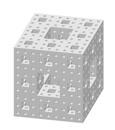
The Menger sponge is obtained from the unit cube by subdividing it into 27 smaller cubes each with one third the side length, then removing the central cube and the six cubes centered on each face; and then inductively performing the same procedure with each of the remaining 20 smaller cubes; see Figure 1.
The Menger sponge has topological dimension 1, and is the universal compact space with this property, in the sense that any compact Hausdorff space of topological dimension 1 embeds in it.
It is important to understand what kinds of abstract groups arise as subgroups of a random group . However, not all subgroups of a hyperbolic group are of equal importance: the most useful subgroups, and those that tell us the most about the geometry of , are the subgroups with the following properties:
-
(1)
the group itself is something whose intrinsic topological and geometric properties we understand very well; and
-
(2)
the intrinsic geometry of can be uniformly compared with the extrinsic geometry of its embedding in .
In other words, we are interested in well-understood groups which are quasi-isometrically embedded in .
A finitely generated quasi-isometrically embedded subgroup of a hyperbolic group is itself hyperbolic, and therefore finitely presented. The inclusion of into induces an embedding of Gromov boundaries . Thus if is a random group, the boundary of has dimension at most 1, and by work of [Kapovich–Kleiner(2000)], there is a hierarchical description of all possible .
First of all, if is disconnected, then one knows by [Stallings(1968)] that splits over a finite group. Second of all, if is connected and contains a local cut point, then one knows by [Bowditch(1998)] that either is virtually a surface group, or else splits over a cyclic group. Thus, apart from the Menger sponge itself, understanding hyperbolic groups with boundary of dimension at most 1 reduces (in some sense) to the case that is a Cantor set, a circle, or a Sierpinski carpet — i.e. one of the “faces” of the Menger cube. The Sierpinski carpet is universal for 1-dimensional compact Hausdorff planar sets of topological dimension 1. Thus one is naturally led to the following fundamental question, which as far as we know was first asked explicitly by François Dahmani:
Question 1.2.1 (Dahmani).
Which of the three spaces — Cantor set, circle, Sierpinski carpet — arise as the boundary of a quasiconvex subgroup of a random group?
Combining the main theorem of this paper with the results of [Calegari–Walker(2015)] gives a complete answer to this question:
Answer.
All three spaces arise in a random group as the boundary of a quasiconvex subgroup (with overwhelming probability).
This is true in the few relators model with any positive number of relators, or the density model at any density less than a half. The situation is summarized as follows:
-
(1)
is a Cantor set if and only if is virtually free (of rank at least 2); we can thus take . The existence of free quasiconvex subgroups in arbitrary (nonelementary) hyperbolic groups is due to Klein, by the ping-pong argument.
-
(2)
is a circle if and only if is virtually a surface group (of genus at least 2); we can thus take . The existence of surface subgroups in random groups (with overwhelming probability) is proved by [Calegari–Walker(2015)], Theorem 6.4.1.
-
(3)
is a Sierpinski carpet if is virtually the fundamental group of a compact hyperbolic 3-manifold with (nonempty) totally geodesic boundary; and if the Cannon conjecture is true, this is if and only if — see [Kapovich–Kleiner(2000)]. The existence of such 3-manifold subgroups in random groups (with overwhelming probability) is Theorem 6.2.1 in this paper.
Explicitly, we prove:
3-Manifolds Everywhere Theorem 6.2.1.
Fix . A random -generator group — either in the few relators model with relators, or the density model with density — and relators of length contains many quasi-isometrically embedded subgroups isomorphic to the fundamental group of a hyperbolic 3-manifold with totally geodesic boundary, with probability for some .
Our theorem applies in particular in the few relators model where . In fact, if one fixes , and starts with a random 1-relator group , one can construct a quasiconvex 3-manifold subgroup (of the sort which is guaranteed by the theorem) which stays injective and quasiconvex (with overwhelming probability) as a further relators are added.
1.3. Commensurability
Two groups are said to be commensurable if they have isomorphic subgroups of finite index. Commensurability is an equivalence relation, and it is natural to wonder what commensurability classes of 3-manifold groups arise in a random group.
We are able to put very strong constraints on the commensurability classes of the 3-manifold groups we construct. It is probably too much to hope to be able to construct a subgroup of a fixed commensurability class. But we can arrange for our 3-manifold groups to be commensurable with some element of a family of finitely generated groups given by presentations which differ only by varying the order of torsion of a specific element. Hence our 3-manifold subgroups are all commensurable with Kleinian groups of bounded convex covolume (i.e. the convex hulls of the quotients have uniformly bounded volume). Explicitly:
Commensurability Theorem 7.0.2.
A random group at any density or in the few relators model contains (with overwhelming probability) a subgroup commensurable with the Coxeter group for some , where is the Coxeter group with Coxeter diagram
The Coxeter group is commensurable with the group generated by reflections in the sides of a regular super ideal tetrahedron — one with vertices “outside” the sphere at infinity — and with dihedral angles .
1.4. Plan of the paper
We now describe the outline of the paper.
As discussed above, our random groups come together with the data of a finite presentation
From such a presentation we can build in a canonical way a 2-complex with 1-skeleton , where is a wedge of circles, and is obtained by attaching disks along loops in corresponding to the relators; so .
Our 3-manifold subgroups arise as the fundamental groups of 2-complexes that come with immersions taking (open) cells of homeomorphically to cells of . Thus, for every 2-cell of , the attaching map of its boundary to the 1-skeleton factors through a map onto one of the relators of the given presentation of .
One way to obtain such a complex is to build a 1-complex as a quotient of a collection of circles together with an immersion where is the 1-skeleton of , and the map takes each component to the image of a relator. We call data of this kind a spine. In § 2 we describe the topology of spines and give sufficient combinatorial conditions on a spine to ensure that is homotopic to a 3-manifold.
Since is a rose whose edges are endowed with a choice of orientation and labelling by the generators , we will usually encode a map of graphs by labelling (oriented) edges by , in the spirit of [Stallings(1983)]. As usual, if an oriented edge of is labelled then the oriented edge with the reverse orientation is labelled . Note that there is a simple condition to ensure that such a map is an immersion: one simply requires that no two oriented edges of incident at the same vertex have the same label. We call such a graph folded (also in the spirit of [Stallings(1983)]).
In § 3 we prove the Thin Spine Theorem, which says that we can build such a spine , satisfying the desired combinatorial conditions, and such that every edge of the 1-skeleton is long. Here we measure the length of edges of by pulling back length from under the immersion , where each edge of is normalized to have length . In fact, if we let denote the 1-relator group
with associated 2-complex which comes with a tautological inclusion , then our thin spines have the property that the immersion factors through .
For technical reasons, rather than working with a random relator , we work instead with a relator which is merely sufficiently pseudorandom (a condition concerning equidistribution of subwords with controlled error on certain scales), and the theorem we prove is deterministic. Of course, the definition of pseudorandom is such that a random word will be pseudorandom with very high probability.
Explicitly, we prove:
Thin Spine Theorem 3.1.2.
For any there is and so that, if is -pseudorandom and is the 2-complex associated to the presentation , then there is a spine over for which is a union of 648 circles (or 5,832 circles if ), and every edge of has length at least .
This is by far the longest section in the paper, and it involves a complicated combinatorial argument with many interdependent steps. It should be remarked that one of the key ideas we exploit in this section is the method of random matching with correction: randomness (actually, pseudorandomness) is used to show that the desired combinatorial construction can be performed with very small error. In the process, we build a reservoir of small independent pieces which may be adjusted by various local moves in such a way as to “correct” the errors that arose at the random matching step. Similar ideas were also used by [Kahn–Markovic(2011)] in their proof of the Ehrenpreis Conjecture, by [Calegari–Walker(2015)] in their construction of surface subgroups in random groups, and by [Keevash(2014)] in his construction of General Steiner Systems and Designs. Evidently this method is extremely powerful, and its full potential is far from being exhausted.
The Thin Spine Theorem can be summarized by saying that as a graph, has bounded valence, but very long edges. This means that the image of in induced by the inclusion is very “sparse”, in the sense that the ball of radius in contains elements of , where we can take as big as we like. This has the following consequence: when we obtain as a quotient of by adding as a relator, we should not kill any “accidental” elements of , so that the image of will be isomorphic to , a 3-manifold group.
This idea is fleshed out in § 4, and shows that random 1-relator groups contain 3-manifold subgroups, although at this stage we have not yet shown that the 3-manifold is of the desired form. The argument in this section depends on a so-called bead decomposition, which is very closely analogous to the bead decomposition used to construct surface groups by [Calegari–Walker(2015)], and the proof is very similar.
In § 5 we show that the 3-manifold homotopic to the 2-complex is acylindrical; equivalently, that it is homeomorphic to a compact hyperbolic 3-manifold with totally geodesic boundary. This is a step with no precise analog in [Calegari–Walker(2015)], but the argument is very similar to the argument showing that is injective in the 1-relator group . There are two kinds of annuli to rule out: those that use 2-cells of , and those that don’t. The annuli without 2-cells are ruled out by the combinatorics of the construction. Those that use 2-cells are ruled out by a small cancellation argument which uses the thinness of the spine. So at the end of this section, we have shown that random 1-relator groups contain subgroups isomorphic to the fundamental groups of compact hyperbolic 3-manifolds with totally geodesic boundary.
Finally, in § 6, we show that the subgroup stays injective as the remaining random relators are added. The argument here stays extremely close to the analogous argument in [Calegari–Walker(2015)], and depends (as [Calegari–Walker(2015)] did) on a kind of small cancellation theory for random groups developed by [Ollivier(2007)]. This concludes the proof of the main theorem.
A further section § 7 proves the Commensurability Theorem. The proof is straightforward given the technology developed in the earlier sections.
2. Spines
2.1. Trivalent fatgraphs and spines
Before introducing spines, we first motivate them by describing the analogous, but simpler, theory of fatgraphs.
A fatgraph is a (simplicial) graph together with a cyclic ordering of the edges incident to each vertex. This cyclic ordering can be used to canonically “fatten” the graph so that it embeds in an oriented surface with boundary, in such a way that deformation retracts down to . Under this deformation retraction, the boundary maps to in such a way that the preimage of each edge of consists of two intervals in , each mapping homeomorphically to , with opposite orientations.
Abstractly, the data of a fatgraph can be given by an ordinary graph , a 1-manifold , and a locally injective simplicial map of (geometric) “degree 2”; i.e. such that each edge of is in the image of two intervals in . The surface arises as the mapping cone of . If one orients and insists that the preimages of each edge have opposite orientations, the result is a fatgraph and an oriented surface as above. If one does not insist on the orientation condition, the mapping cone need not be orientable. Attaching a disk along its boundary to each component of produces a closed surface, which we denote .
We would like to discuss a more complicated object called a spine, for which the analog of is a 2-complex homotopy equivalent to a compact 3-manifold with boundary. The 2-complex will arise by gluing 2-dimensional disks onto the components of a 1-manifold , and then attaching these disks to the mapping cone of an immersion where is a 4-valent graph, and the map is subject to certain local combinatorial constraints.
The first combinatorial constraint is that the map should be “degree 3”; that is, the preimage of each edge of should consist of three disjoint intervals in , each mapped homeomorphically by .
Since is 4-valent, at each vertex of we have 12 intervals in that map to the incident edges; these 12 intervals should be obtained by subdividing 6 disjoint intervals in , where the dividing point maps to . Since is an immersion, near each dividing point the given interval in runs locally from one edge incident to to a different one. There are three local models (up to symmetry) of how six edges of can locally run over a 4-valent vertex of so that they run over each incident edge (in ) to three times (this notion of “local model” is frequently called a Whitehead graph in the literature). These three local models are illustrated in Figure 2.
2pt
\pinlabelType A at -200 0
\endlabellist
The third local model is distinguished by the property that for each pair of edges of adjacent to , there is exactly one interval in running over from one edge to the other. We say that such a local model is good. The second combinatorial constraint is that the local model at every vertex of is good.
If is good, and is the mapping cone of , then the 2-complex can be canonically thickened to a 3-manifold, since a neighborhood of the mapping cone near a vertex embeds in in such a way that the tetrahedral symmetry of the combinatorics is realized by symmetries of the embedding. Similarly, along each edge the dihedral symmetry is realized by the symmetry of the embedding. The restriction of this thickening to each component of is the total space of an -bundle over the circle; we say that is co-oriented if each of these -bundles is trivial. The third combinatorial constraint is that is co-oriented.
Definition 2.1.1.
A spine is the data of a compact 1-manifold and a 4-valent graph , together with a co-oriented degree 3 immersion whose local model at every vertex of is good. If is a spine, we denote the mapping cone by , and by the 2-complex obtained by capping each component of in off by a disk.
Lemma 2.1.2 (Spine thickens).
Let be a spine. Then is canonically homotopy equivalent to a compact 3-manifold with boundary.
Proof.
We have already seen that has a canonical thickening to a compact 3-manifold in such a way that the restriction of this thickening to each component of is an -bundle. The total space of this -bundle is an annulus embedded in the boundary of , and we may therefore attach a 2-handle with core the corresponding component of providing this -bundle is trivial. But that is exactly the condition that should be co-oriented. ∎
By abuse of notation, we call the thickening of .
2.2. Tautological immersions
Now let’s fix and a free group on fixed generators. Let be a rose for ; i.e. a wedge of (oriented) circles, with a given labeling by the generators of . Let be a random group (in whatever model) at length . Each relator is a cyclically reduced word in , and is realized geometrically by an immersion of an oriented circle . Attaching a disk along each such circle gives rise to the 2-complex described in the introduction with .
Definition 2.2.1.
A spine over is a spine together with an immersion such that for each component of , there is some relator and a simplicial homeomorphism for which .
The existence of the simplicial homeomorphisms lets us label the components by the corresponding relators in such a way that the map has the property that the preimages of each edge of get the same labels, at least if we choose orientations correctly, and use the convention that changing the orientation of an edge replaces the label by its inverse. So we can equivalently think of the labels as living on the oriented edges of . Notice that the maps , if they exist at all, are uniquely determined by (at least if the presentation is not redundant, so that no relator is equal to a conjugate of another relator or its inverse).
Evidently, if , is a spine over , the immersion extends to an immersion of the thickening , that we call the tautological immersion.
Our strategy is to construct a spine over for which is homotopy equivalent to a compact hyperbolic 3-manifold with geodesic boundary, and for which the tautological immersion induces a quasi-isometric embedding on .
3. The Thin Spine Theorem
The purpose of this section is to prove the Thin Spine Theorem, the analog in our context of the Thin Fatgraph Theorem from [Calegari–Walker(2015)].
In words, this theorem says that if is a sufficiently long random cyclically reduced word in giving rise to a random 1-relator group with associated 2-complex , then with overwhelming probability, there is a good spine over for which every edge of is as long as we like; colloquially, the spine is thin.
For technical reasons, we prove this theorem merely for sufficiently “pseudorandom” words, to be defined presently.
3.1. Pseudorandomness
Instead of working directly with random chains, we use a deterministic variant called pseudorandomness.
Definition 3.1.1.
Let be a cyclically reduced cyclic word in a free group with generators. We say is -pseudorandom if the following is true: if we pick any cyclic conjugate of , and write it as a reduced product of reduced words of length (and at most one word of length )
(so ) then for every reduced word of length in , there is an estimate
Here the factor is simply the number of reduced words in of length . Similarly, we say that a collection of reduced words each of length is -pseudorandom if for every reduced word of length in the estimate above holds.
For any , a random reduced word of length will be -pseudorandom with probability for a suitable constant . This follows immediately from the standard Chernoff inequality for the stationary Markov process that produces a random reduced word in a free group (cf. [Calegari–Walker(2015), Lemma 3.2.2]).
With this definition in place, the statement of the Thin Spine Theorem is:
Theorem 3.1.2 (Thin Spine Theorem).
For any there is and so that, if is -pseudorandom and is the 2-complex associated to the presentation , then there is a spine over for which is a union of 648 circles (or 5,832 circles if ), and every edge of has length at least .
The strange appearance of the number 648 (or 5,832 for ) in the statement of this theorem reflects the method of proof. First of all, observe that if is any spine, then since has degree 3, the total length of is divisible by 3. If this spine is over , then each component of has length , and if we make no assumptions about the value of mod 3, then it will be necessary in general for the number of components of to be divisible by 3.
Our argument is to gradually glue up more and more of , constructing as we go. At an intermediate stage, the remainder to be glued up consists of a collection of disjoint segments from , and the power of our method is precisely that this lets us reduce the gluing problem to a collection of independent subproblems of uniformly bounded size. But each of these subproblems must involve a subset of of total length divisible by 3 or 6, and therefore it is necessary to “clear denominators” (by taking 2 or 3 disjoint copies of the result of the partial construction) several times to complete the construction (in the case of rank 2 one extra move might require a further factor of 9).
Finally, at the last step of the construction, we take 2 copies of and perform a final adjustment to satisfy the co-orientation condition.
The remainder of this section is devoted to the proof of Theorem 3.1.2.
3.2. Graphs and types
Let be a labeled graph consisting of 648 disjoint cycles (or 5,832 disjoint cycles if ), each labeled by . We will build the spine and the map in stages. We think of as a quotient space of , obtained by identifying segments in with the same labels. So the construction of proceeds by inductively identifying more and more segments of , so that at each stage some portion of has been “glued up” to form part of the graph , and some remains still unglued.
We introduce the following notation and terminology. Let be a single cycle labeled . At the th stage of our construction, we deal with a partially glued graph , constructed from a certain number of copies of via certain ungluing and gluing moves. At each stage, is equipped with a labelling, defining a map . We will always be careful to ensure that is folded, i.e. that the map is an immersion. The glued subgraph of is denoted by , and the unglued subgraph by . Shortly, the unglued subgraph will be expressed as the disjoint union of two subgraphs: the remainder and the reservoir .
Each of these graphs are thought of as metric graphs, whose edges have lengths equal to the length of the words that label them. The mass of a metric graph is its total length, denoted by . The type of a graph refers to the collection of edge labels (which are reduced words in ) associated to each edge. A distribution on a certain set of types of graphs is a map that assigns a non-negative number to each type; it is integral if it assigns an integer to each type. We use this terminology without comment in the sequel.
The following properties will remain true at every stage of our construction. The branch vertices of (those of valence greater than two) have valence four. The length of each edge will always be at least . We will be careful to ensure that any branch vertex in the interior of the glued part is good in the sense of Section 2. Vertices in the intersection of the glued and unglued parts, , will always be branch vertices, and will be such that one adjacent edge is in , and the remaining three adjacent edges in have distinct labels.
In particular, we start with and . At the last stage of our construction we will have constructed from 324 copies of (or 2,916 if ), which is completely glued up; that is, and . Finally, the modification in Section 3.12 doubles the mass of in order to ensure that the co-orientation condition is satisfied. Taking to be the result of this construction and to be the quotient map proves the theorem.
3.3. Football bubbles
We will regard and as constants. The first step of the construction is to pick some very big constant where still (we will explain in the sequel how to choose and big enough) so that is odd.
Let be the remainder when is divided by . By pseudorandomness, we may find three subsegments in of reduced form
where are single edges, such that the labels are all distinct and are all distinct, and the length of is . We take three copies of , fix one of the above subsegments in each copy, and glue the parts of these subsegments labeled together to obtain . Note that the requirement that the labels are distinct ensures that remains folded. We summarize this in the following lemma.
Lemma 3.3.1.
After gluing three copies of along subsegments of length we obtain , with the property that the length of each edge of the unglued subgraph is congruent to modulo . The glued subgraph is a segment of length .
We next decompose the unglued subgraph into disjoint segments of length separated by segments of length . Call the segments of length long strips and the segments of length short strips. Now further decompose each long strip into alternating segments of length ; we call the odd numbered segments sticky and the even numbered segments free.
We will usually denote a long strip by
where the are sticky, the (or etc) are free, and all are of length . When we also need to include the neighboring short strips, we will usually extend this notation to
where and (or etc) denote the neighboring short strips.
Definition 3.3.2.
Three long strips are compatible if they (and their adjoining short strips) are of the form
(i.e. if their sticky segments agree) and if for even (i.e. for the free segments) the letters adjacent to each or disagree.
A compatible triple of long strips can be bunched — i.e. the sticky segments can be glued together in threes, creating football bubbles, each football consisting of the three segments (for some ) arranged as the edges of a theta graph. See Figure 3.
2pt
\endlabellist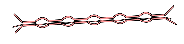
By pseudorandomness, a proportion of approximately of the long strips in can be partitioned into compatible triples. Then each compatible triple can be bunched, creating a reservoir of footballs (i.e. the theta graphs appearing as bubbles) and a remainder, consisting of the union of the unglued pieces (except for the footballs). In what follows, we will denote the remainder in by and the reservoir by .
We summarize this observation in the next lemma. By an extended long strip, we mean a long strip, together with half the adjacent short strips.
Lemma 3.3.3.
Suppose that , and that is sufficiently large and is sufficiently small. After bunching compatible triples in the unglued graph we obtain the partially glued graph with the following properties.
-
(1)
The total mass of the unglued subgraph satisfies
for a constant .
-
(2)
We can decompose the unglued subgraph as a disjoint union . The reservoir is a disjoint union of bubbles.
-
(3)
The mass of the remainder satisfies
as long as .
-
(4)
The distribution of the types of bubbles in the reservoir is within of a constant distribution (independent of and ).
Proof.
The number of types of extended long strips is for some constant . The unglued subgraph is still -pseudorandom, containing a union of
extended long strips. By pseudorandomness, we may restrict to a subset of mass at least so that the types of extended long strips in are exactly uniformly distributed. (Here we use that .) We then randomly choose a partition into compatible triples, and perform bunching, to produce .
As described above, the unglued subgraph is naturally a disjoint union of the remainder and the reservoir . The remainder consists, by definition, of the union of and the short strips in (after gluing). Hence
which is as long as .
Bunching uniformly distributed long strips at random induces a fixed distribution on subgraphs of bounded size. This justifies the final assertion. ∎
3.4. Super-compatible long strips
At this point, we have bunched all but of the long strips into triples. In particular, for sufficiently small , the number of bunched triples is far larger than the number of unbunched long strips. We will now argue that we may, in fact, adjust the construction so that every long strip is bunched. The advantage of this is that after this step, the unglued part consists entirely of the reservoir (a union of football bubbles) and a remainder consisting of a trivalent graph in which every edge has length exactly . The key to this operation is the idea a super-compatible 4-tuple of long segments.
Definition 3.4.1.
Four long strips are super-compatible if they are of the form
(i.e. if their sticky segments agree) and if for even (i.e. for the free segments) the initial and terminal letters of disagree. Alternatively, such a 4-tuple is super-compatible if every sub-triple is compatible.
Remark 3.4.2.
Notice that the existence of super-compatible 4-tuples depends on rank . An alternative method to eliminate unbunched long strips in rank 2 is given in § 3.13.
Lemma 3.4.3.
Let be as above. As long as and is sufficiently small (depending on ), one can injectively assign to each long strip in the remainder a bunched triple in such that the quartet is super-compatible.
Proof.
Let be an unglued long strip. As long as , it is clear that there is at least one type of bunched triple such that is super-compatible. The total number of types of bunched triples is for some . Therefore, the proportion of bunched triples that are super-compatible with is at least . On the other hand, the proportion of long strips that are unbunched is . Therefore, we can choose a bunched triple for every unbunched long strip as long as . ∎
By the previous lemma, we may assign to each unglued long strip in the remainder a glued triple such that is super-compatible. We may re-bunch these into the four possible compatible triples that are subsets of our super-compatible 4-tuple, viz:
The result of performing this operation on every long strip in the remainder yields the new partially glued graph .
Lemma 3.4.4.
Take 3 copies of as above, and suppose that is sufficiently large and is sufficiently small. After choosing super-compatible triples and re-bunching so that every long strip is bunched, we produce the partially glued graph with the following properties.
-
(1)
The partially glued graph consists of a glued subgraph , a reservoir , and a remainder .
-
(2)
The reservoir consists of football bubbles and its mass is bounded below by
-
(3)
The remainder is a trivalent graph with each edge of length , and its mass is bounded above by
-
(4)
Let be the uniform distribution on types of bubbles. Then for any type of bubble, the proportion of bubbles in the reservoir of type is within of .
Proof.
Consider , the unglued subgraph of . Then is the union of three arcs, of total mass , where is the number of long strips in . Recall that is constructed from three copies of , and that for each long strip, one short strip goes into the remainder, and go into the reservoir. Therefore, we have that
and
Finally, we need to check that the re-gluing only has a small effect on the distribution of bubble types. Recall that the unglued long strips in are precisely the images of the unglued long strips in , which is of mass at most .
Taking three copies of each of these and three copies of a super-compatible triple, re-bunching produces four new bunched triples. In particular, for each three unbunched long strips, we destroy bubbles and replace them with new bubbles of different types. The proportion of unglued long strips was at most . It follows that the proportional distribution of each bubble type was altered by at most , so the final estimate follows. ∎
3.5. Inner and outer reservoirs and slack
As their name indicates, the bubbles in the reservoir will be held in reserve until a later stage of the construction to glue up the remainder. Some intermediate operations on the remainder have “boundary effects”, which might disturb the neighboring bubbles in the reservoir in a predictable way. So it is important to insulate the remainder with a collar of bubbles which we do not disturb accidentally in subsequent operations.
Fix a constant and divide each long strip in into two parts: and inner reservoir, consisting of an innermost sequence of consecutive bubbles of length times the length of the long strip, and an outer reservoir, consisting of two outer sequences of consecutive bubbles of length . The number is called the slack. Boundary effects associated to each step that we perform will use up bubbles from the outer reservoir and at most halve the slack. Since the number of steps we perform is uniformly bounded, it follows that — provided is sufficiently large — even at the end of the construction we will still have a significant outer reservoir with which to work.
3.6. Adjusting the distribution
After collecting long strips into compatible triples, the collection of football bubbles in the reservoir is “almost equidistributed”, in the sense that the mass of any two different types of football is almost equal (up to an additive error of order ). However, it is useful to be able to adjust the pattern of gluing in order to make the distribution of football bubbles conform to some other specified distribution (again, up to an additive error of order ).
This operation has an unpredictable effect on the remainder, transforming it into some new 3-valent graph (of some possibly very different combinatorial type); however, it preserves the essential features of the remainder that are known to hold at this stage of the construction: every edge of the remainder (after the operation) has length exactly ; and the total mass of the remainder before and after the operation is unchanged (so that it is still very small compared to the mass of any given football type).
Let be a probability measure on the set of all football types, with full support — i.e. so that is strictly positive on every football type. (In the sequel, will be the cube distribution described below, but that is not important at this stage.) Suppose we have three long strips of the form
so that the result of the gluing produces bunches each with the label (for odd), and football bubbles each with the label (for even). We think of the as unordered triples — i.e. we only think of the underlying football as an abstract graph with edge labels up to isomorphism. A given sequence of labels and (unordered!) football types might arise from three long strips in ways, since there are 6 ways to order each triple .
Let denote the uniform probability measure on football types, and let be chosen to be a multiple of such that for all types. Fix such that . As the notation hints, will turn out to be the slack in the partially glued graph , and we accordingly partition each long strip of into an inner reservoir, of proportional length , and an outer reservoir consisting of two strips of proportional length .
We put all possible triples of long strips labeled as above into a bucket. Next, color each even index in (i.e. those contained in the inner reservoir) black with probability
and color all the remaining indices white, where is short for the measure of the football type (note that our choice of guarantees that the assigned probabilities are never greater than 1).
Now pull apart all the triples of long strips, and match them into new triples according to the following rule: if a given index is white, the corresponding labels should all be different, and equal to (in some order); if a given index is black, the corresponding labels should all be the same, and equal to exactly one of . Then we can glue up to produce footballs exactly for the white labels, and treat the black labels as part of the neighboring sticky segments, so that they are entirely glued up.
We do this operation for each bucket (i.e. for each collection of triples with a given sequence of sticky types and football types ). The net effect is to eliminate a fraction of approximately of the footballs with label ; thus, at the end of this operation, the distribution of footballs is proportional to , with error of order .
Although this adjustment operation can achieve any desired distribution , in practice we will set equal to the cube distribution, to be described in the sequel. In any case, for a fixed choice of distribution , the slack only depends on and , and therefore can be treated as a constant.
We summarize this in the following lemma.
Lemma 3.6.1.
Let be a probability distribution on the set of types of football bubbles and let be sufficiently large. The adjustment described above transforms into a new partially glued graph with the following properties.
-
(1)
The mass of the reservoir is bounded below by a constant depending only on and .
-
(2)
The mass of the remainder is bounded above by
-
(3)
The distribution of football types in the reservoir is proportional to , with error .
-
(4)
The slack is a constant.
Proof.
As noted above, this operation may completely change the combinatorial type of the remainder, but leaves invariant its total mass, and the fact that it is a 3-valent graph with edges of mass . In particular,
and so for sufficiently large . This proves item 2.
We lose a fraction of the reservoir—those indices colored black. An index between and is colored black with probability . Therefore, the proportion of bubbles colored white is bounded below by , and so the mass of the reservoir is bounded below by
Since is a distribution on types of bubbles, depending only on and , the first item holds as long as is sufficiently large.
We next estimate the distributions of the types of bubbles. Before adjustment, the proportion of each type of bubble in the reservoir was within of the uniform distribution. These can be taken to be uniformly distributed between the inner and outer reservoirs. Therefore, after adjustment, the new distribution on bubble types satisfies
and so, as before, since is bounded above in terms of and , the third assertion follows.
The final assertion about the slack is immediate from the construction. ∎
3.7. Tearing up the remainder
At this stage the remainder consists of a 3-valent graph in which every edge has length exactly . The total mass of the remainder is very small compared to the mass of the reservoir, but it is large compared to the size of a single long strip. Furthermore, there is no a priori bound on the combinatorial complexity of a component of the remainder.
We explain how to modify the gluing by a certain local move called a tear111“tear” in the sense of: “There were tears in her big brown overcoat”, which (inductively) reduces the combinatorial complexity of the remainder (which a priori is arbitrarily complicated) until it consists of a disjoint collection of simple pieces. These pieces come in three kinds:
-
(1)
football bubbles;
-
(2)
bizenes: these are graphs with 6 edges and 4 vertices, obtained from a square by doubling two (non-adjacent) edges; and
-
(3)
bicrowns: these are complete bipartite graphs .
The bubbles, bizenes and bicrowns all have edges of length exactly . They are depicted in Figure 4. Note that bizenes doubly cover footballs and bicrowns triply cover footballs. If the labels on a bizene or bicrown happen to be pulled back from the labels on a football bubble via the covering map, then we say that the bizene or bicrown is of covering type.
2pt
\endlabellist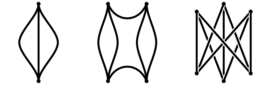
2pt
\endlabellist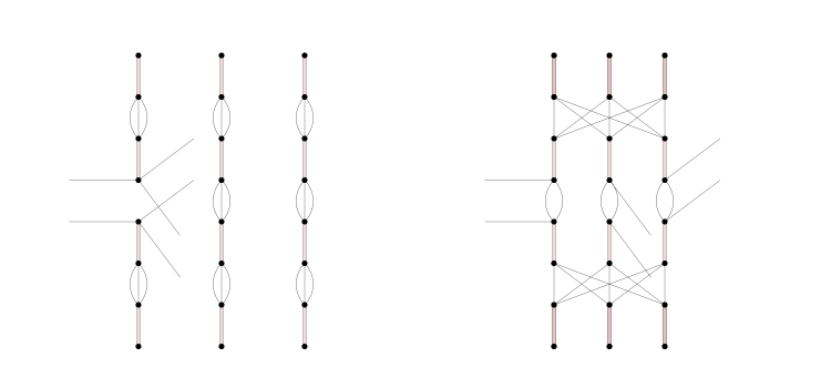
We now describe the operation of tearing. Take two copies of , denoted by and (with vertices, edges and subgraphs of denoted with primes in the obvious manner) and let and be branch vertices of and respectively. These vertices are the ends of disjoint sequences of alternating bunched triples and football bubbles. The tearing operation uses up two (appropriately labeled) sequences of alternating bunched triples and football bubbles, each of length 3. The precise definition of this operation is best given by example, and is illustrated in Figure 5.
On the left of the figure we have the vertices and of and , together with two strings of bubbles. These strings are pulled apart and reglued according to the combinatorics indicated in the figure. Thus, the labels on the bunched triples at each horizontal level should all agree, and the labels on the footballs should be such that the result of the gluing is still folded. The existence of strings of football bubbles with these properties is guaranteed by pseudorandomness and the definition of the long strips.
Thus the operation of tearing uses up 8 footballs (as in the figure), and it has several effects on the remainder. First, is pulled apart at and , producing six new vertices and , and adding two new edges and (from the footballs separating the adjacent bunched triples) joining to . Second, two new bicrowns are created, assembled from the pieces of three identically labeled footballs. Third, the slack at and is reduced to approximately half of its previous value. If the strings of three football segments are taken from the inner half of the outer reservoir, it will reduce the slack at the vertices of at the end of these strips; but the size of the slack at these vertices will stay large.
Lemma 3.7.1.
Suppose that is sufficiently large, is sufficiently small and the partially glued graph is as above. By applying tearing operations to 2 copies of we may build a partially glued graph with the following properties.
-
(1)
The mass of the reservoir is bounded below by a constant depending only on and .
-
(2)
The remainder is a disjoint union of bizenes, and bicrowns of covering type, with mass bounded above by
-
(3)
The distribution of football bubbles of each type is within of the distribution (proportional to ).
-
(4)
The slack satisfies .
Proof.
As described above, we construct from two copies of : let us denote them by and , and likewise denote subgraphs, vertices and edges with primes as appropriate. At each branch vertex of we have three unglued (elementary) edges with labels (pointing away from , say), and one glued edge with label (also pointing away from ). Denote by the short strip in incident at with outgoing label . Let be the corresponding vertex of , which is of course locally isomorphic to .
For each such pair of vertices of and of , we choose a pair of bubbles so that we may perform a tear move at and . In order to do this, we must choose a pair of bubbles , , with certain constraints on the labelings at their branch vertices. We next describe one feasible set of constraints that enables the tearing operation to be performed (there will typically be other possible configurations).
Necessarily, at each branch vertex of and , we need the incident glued (elementary) edge to have (outgoing) label . We will also require that each bubble is a union of three short strips , with the property that at each branch vertex of the outgoing label on the short strip is equal to . Since there are only a finite number of possible local labelings at the branch vertices, and since each type of bubble occurs with roughly equal distribution, there are many bubbles satisfying this condition.
Later in the argument, it will also prove necessary that the strips satisfy certain other constraints (see Lemma 3.10.2 below). For the moment, it suffices that these constraints are mild enough to guarantee the existence of the bubbles .
Given bubbles , for a vertex of , we can perform the tearing operation, in such a way that after tearing, and adjoin and , and adjoin and , and and adjoin and . Note that the resulting graph remains folded, and that the remainder has been replaced by a union of bizenes.
Therefore, in order to perform the tearing operation, we need to find pairs of bubbles as above, where is the number of vertices of . To do this, we divide all football bubbles in the undisturbed segments of the long strips into consecutive runs of seven. For each vertex of the remainder , we need to choose two such runs of a specified type. We furthermore insist on choosing these runs of seven from within the ‘innermost’ part of the ‘outer’ reservoir.
The number is equal to . By pseudorandomness, the number of runs of seven bubbles of a fixed type is bounded below by
(using that is sufficiently small). Half of these runs of seven come from within the innermost part of the outer reservoir. Therefore, as long as is large enough, we can always choose two suitable runs of seven bubbles for each vertex of , as required.
Since is bounded above by a constant (depending on and ) divided by , the distribution of each bubble type has only been changed by .
After performing tears in this way, we obtain a new partially glued graph , with the additional property that the remainder is a disjoint union of bizenes and bicrowns (the latter of covering type). The mass of the remainder is still bounded above by
since three half-edges of are replaced by 36 half-edges of , as shown in Figure 5.
Since, by construction, we only used bubbles in the tearing operation which came from the innermost half of the outer reservoir together with one bubble from the outermost part of the outer reservoir, the slack is no smaller than
as claimed. ∎
3.8. Adjusting football inventory with trades
It will be necessary at a later stage of the argument to adjust the numbers of football pieces of each kind, so that the reservoir itself can be entirely glued up. At this stage and subsequent stages we must be careful to consider not just the combinatorial graph of our pieces, but also their type — i.e. their edge labels.
We now describe a move called a trade which has the following twofold effect:
-
(1)
it reduces the number of footballs of a specified type by 3; and
-
(2)
it transforms four sets of 3 footballs, each of a specified type, into four bicrowns each with the associated covering type.
Moreover, unlike the operation described in § 3.6, the trade operation has no effect on the remainder. Thus, the trade moves can be performed after the tear moves, to correct small errors in the distribution of football types, adjusting this distribution to be exactly as desired.
The trade move is illustrated in Figure 6. We start with three strings of five footballs, each string consisting of the same sequence of five football types in the same orders. We also assume the labels on the three sets of four intermediate sticky segments agree. We pull apart the sticky segments and reglue them in the pattern indicated in the figure, in such a way that four sets of three footballs are replaced with bicrowns. If the three middle footballs are of type then after regluing we can assume that the edges are all together, and similarly for the and edges; thus these triples of edges may by glued up, eliminating the three footballs.
2pt
\endlabellist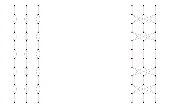
To summarize this succinctly, we introduce some notation. For a type of football bubble, we denote by the corresponding covering type of bicrown. For a distribution on football bubbles and bicrowns of covering type, we denote by the following distribution on football bubbles.
Lemma 3.8.1.
Let the partially glued graph be as above and suppose that is sufficiently small. There is a constant with the following property. Let be the distribution of bubble types in and let be any integral distribution on bubble types such that, for each type ,
Then we may apply trades as above to 3 copies of the partially glued graph to produce a new partially glued graph such that:
-
(1)
the induced distribution on bubbles and bicrowns satisfies ;
-
(2)
the mass of the remainder is bounded above by
-
(3)
the slack satisfies .
Proof.
Let be the distribution on football bubbles and bicrowns derived from . From the upper bound on the total mass of the remainder, it follows that .
We divide the inner half of the outer reservoir into strips of five contiguous football bubbles, and call a football bubble fifth if it lies in the center of such a quintuple. Let denote the distribution of fifth football bubbles in the inner half of the outer reservoir .
Recall that, in the outer reservoir, the bubbles are distributed within of the uniform distribution. Therefore, for any football bubble type , (where is the uniform distribution, scaled appropriately). In particular, taking sufficiently large and sufficiently small, we have
for some constant . Hence the hypothesis of the lemma implies that for every type of football bubble. If is sufficiently large then it follows further that for every type .
Consider each bubble in the center of a quintuple in the outer reservoir of type . We color the bubble black with probability and white otherwise.
We now construct from three copies of , by performing a trade at each bubble colored black. Taking three copies of triples the number of each bubble type. The lemma is phrased so that replacing three bubbles of a given type by a bicrown of corresponding covering type is neutral. The only remaining effect of a trade is then to remove exactly three bubbles of the central type. This proves the lemma. ∎
In the sequel, we will apply this lemma with a particular distribution , described in Lemma 3.11.1 below.
3.9. Cube and prism moves
We have two more gluing steps: a small mass of bicrowns and bizenes must be glued up with footballs (drawn from an almost equidistributed collection of much larger mass), then the distribution of the footballs can be corrected by trades so that they are perfectly evenly distributed, and finally an evenly distributed collection of footballs (i.e. a collection with exactly the same number of footballs with each possible label) must be entirely glued up. We next describe three moves which will enable us to glue up bubbles, bizenes and bicrowns.
3.9.1. The cube move
The idea is very simple: four footballs with appropriate edge labels can be draped over the 1-skeleton of a cube in a manner invariant under the action of the Klein 4-group, and then glued up according to how they match along the edges of the cube. This is indicated in Figure 7.
2pt
\endlabellist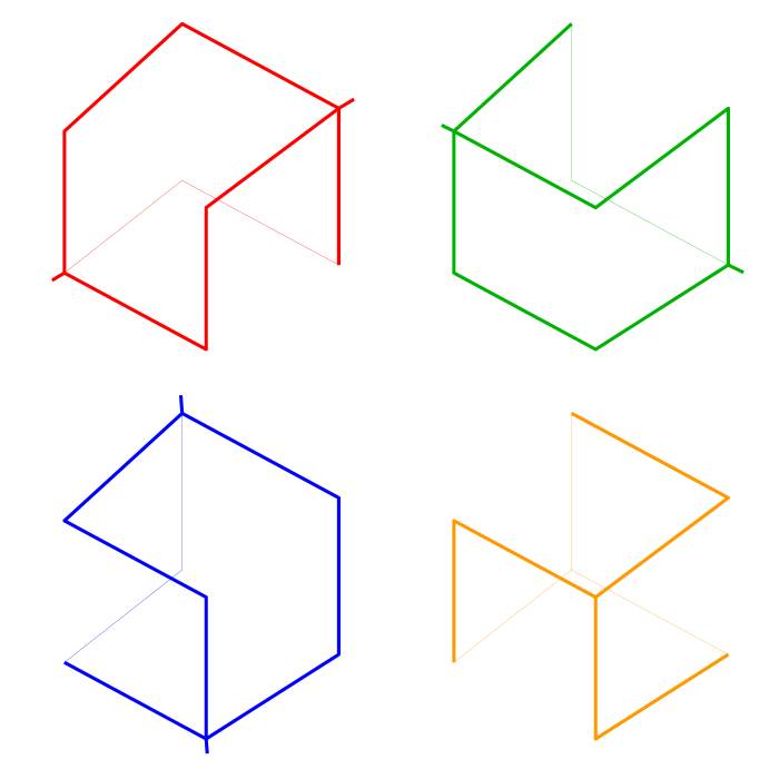
We next give an algebraic description of the cube move in terms of covering spaces of graphs, which enables us to give a precise description of the various coverings of the cube moves that we will also need.
Consider two theta-graphs, and . The three edges of are denoted by (oriented so they all pointing in the same direction), and likewise the three edges of are denoted by . We consider the immersion which maps the edges of to concatenations of edges of as follows:
(as usual, denotes with the opposite orientation etc). To enable us to reason group-theoretically, we set and , and similarly and . Fixing base points at the initial vertices of all the edges, is the free group on and is the free group on . We immediately see that the immersion induces the identifications
and
The graph should be thought of as a bubble, and the graph as a pattern for gluing it up. In what follows, we will describe various covering spaces . The fibre product of the maps and , together with the induced map , will then describe various gluing patterns for (covering spaces of) unions of bubbles.
We first start with the cube move itself. Consider the natural quotient map , where is the Klein 4-group. The corresponding covering space is a cube with quotient graph . Note that the deck group acts freely on the cube , freely permuting the diagonals. Since , the fibre product is a disjoint union of four copies of , each spanning a diagonal in the cube and freely permuted by . In particular, the map precisely defines the cube move.
3.9.2. Gluing bizenes
We next describe a gluing move for bizenes. Consider the quotient map from to the dihedral group defined by and , and let be the covering space of corresponding to the kernel of . Since factors through , is a degree-two covering space of the cube (the graph is in fact the 1-skeleton of an octagonal prism). We next calculate the restriction of to :
while
The covering space of corresponding to the restriction of is therefore a bizene. It follows that the fibre product map
describes a double cover of the cube move, which glues four bizenes along an octagonal prism. We will call this an 8-prism move.
3.9.3. Gluing bicrowns
Finally, we describe a gluing move for bicrowns. Consider the quotient map defined by and . Then, as before, since factors through , the kernel of corresponds to a regular covering space of degree three (in fact, is isomorphic to the 1-skeleton of a dodecagonal prism). Again, we calculate the restriction of to , and find that
(an element of order 3). The covering space of corresponding to the restriction of is therefore a bicrown. In particular, the fibre product map
describes a triple cover of the cube move, which glues four bicrowns along a dodecagonal prism. We will call this a 12-prism move.
3.10. Creating bizenes and bicrowns
To complete the proof of the Thin Spine Theorem, we need to glue up the remaining small mass (of order ) of bizenes and bicrowns using prism moves, before gluing up the remaining football bubbles using cube moves. We shall see that trades provide us with enough flexibility to do this, as long as is large enough. However, since prism moves require that bizenes are glued up with bizenes and our bicrowns are glued up with bicrowns, and yet the reservoir consists only of football bubbles, we will need a move that turns football bubbles into bizenes and bicrowns of given types.
3.10.1. Bicrown assembly
Since the bicrowns that we need to assemble are all of covering type, it is straightforward to construct them from football bubbles. Given a bicrown of covering type , covering a football bubble of type , there is a move which takes as input three identical triples of bubbles each of type , and transforms them into three bicrowns of type , without any other changes to the unglued subgraph.
The following lemma is an immediate consequence of the fact that a 12-prism triply covers a cube.
Lemma 3.10.1.
For every bicrown of covering type there exist three more bicrowns of covering type such that the four bicrowns together can be glued with a 12-prism move.
3.10.2. Bizene assembly
Bizene assembly is more subtle, because the bizenes that we need are more general than simply of covering type. We assemble bizenes using the following move.
Consider an adjacent pair of bubbles of type and , separated by a sticky strip of type . Suppose also that the second bubble (of type ) is followed by a further sticky strip also of type . Consider also a second pair of bubbles, of the same type but with the two bubbles swapped. From these two pairs we may construct two bizenes of the same type. The pairs of edges with the same start and end points are labeled and , while the edges joining one pair to the other are labeled and .
The bizenes that we may assemble in this way satisfy some constraints, arising from the fact that both the ends of the following triples must all be compatible with the start of : , , , . In the rank-two case, this creates especially strong constraints, which (up to relabeling) can be simply stated as requiring that the ends of , and should be equal to the ends of , and respectively. We shall call such a bizene constructible.
Just as the bizenes that we can construct are constrained, so the bizenes that we need to glue up from the remainder are also of a special form. Indeed, in the proof of Lemma 3.7.1 we were free to choose the interiors of the bubbles and in any way.
Lemma 3.10.2.
There exist choices of the bubble types and in the proof of Lemma 3.7.1 such that the resulting remainder bizenes can be glued with a prism move to three constructible bizenes.
Proof.
Such a choice is illustrated in Figure 8. Note that the constrained vertices of the yellow, green and blue constructible bizenes are disjoint from each other and from the determined arcs of the red remainder bizene. Therefore, we can start by labeling the two arcs and the constrained vertices, and then label the rest of the 8-prism in any way we want. Doing this for each determines the bubble types and . ∎
3.11. Gluing up the remainder
In this section we use the moves described above to completely glue up the remainder and the reservoir. But first we will address two important details which we have hitherto left undefined: the distributions (of Lemma 3.6.1) and (of Lemma 3.8.1).
We first describe ‘cubical distributions’. Consider any distribution on the set of types of cubes with side length . The cube move associates to each type of cube a collection of four types of football bubbles. The push forward of any distribution to the set of types of football bubbles is called a cubical distribution. In particular, if is the uniform distribution on the set of types of cubes then we call the push forward the uniform cubical distribution, or just the cube distribution for brevity.
In Subsection 3.6 above we may take to be the cube distribution, so that the set of football bubbles in the reservoir is within of , a distribution proportional to the cube distribution.
We next address the distribution from Lemma 3.8.1. It consists of two parts: any cubical distribution , and a bizene correction distribution . That is, . So we need to describe the bizene correction distribution.
The remainder consists of (remainder) bizenes and bicrowns. By Lemma 3.10.2, to each remainder bizene we associate (some choice of) three constructible bizenes. Each constructible bizene can in turn be constructed from a pair of types of football bubble. Thus, to each remainder bizene we associate six football bubbles. Summing over all bizenes in the remainder defines the distribution .
In order to apply Lemma 3.8.1, we need to check that there is a cubical distribution such that satisfies the hypotheses of the lemma.
Lemma 3.11.1.
If is sufficiently large then there exists a cubical distribution such that the integral distribution satisfies
(where is the constant from Lemma 3.8.1). Furthermore, as long as is sufficiently large, we may take to be integral.
Proof.
Since the mass of the remainder is and is bounded below, it follows that for each type of football bubble, so it suffices to show that there is an integral cubical distribution satisfying
By the construction of , there is a cubical distribution such that . Choose a rational . As long as is sufficiently large we will also have that , and it follows that satisfies the required condition. Furthermore, if is sufficiently large then can be chosen so that is integral. ∎
We can now glue up all the bizenes, using bizene assembly and the 8-prism move.
Lemma 3.11.2.
Let be as in Lemma 3.8.1, using the distribution from Lemma 3.11.1. Then we may apply 8-prism moves to 2 copies of to produce a partially glued graph such that:
-
(1)
every component of the remainder is a bicrown of covering type;
-
(2)
the total mass of the remainder satisfies ;
-
(3)
if is the distribution of bubbles and bicrowns in then is cubical;
-
(4)
the slack satisfies .
Proof.
Let be the distribution of constructible bizenes required to glue up the remainder bizenes in . Take two copies of . Using the bizene assembly move, we construct exactly new bizenes of each type from the inner half of the outer reservoir. From the definition of we may now glue up all the bizenes using the 8-prism move. By the construction of , it follows that and so is cubical.
Since the total mass of bicrowns was in , the same is true in . ∎
The next lemma completes the proof of the Thin Spine Theorem, except for a small adjustment needed to correct co-orientation, in the case when .
Lemma 3.11.3.
From 3 copies of as above, we can construct a graph in which the unglued subgraph is empty.
Proof.
For each bicrown (of covering type), there exist bicrowns of covering type (where ) such that the for can be glued up using a 12-prism move. Three copies of each of these can in turn be constructed from three consecutive copies of bubbles , using the bicrown assembly move from Lemma 3.10.1. Let be the distribution on bubble types that, for each bicrown of type in the remainder, counts three bubbles of each type . Note that, because all the bicrowns are of covering type and the 12-prism move covers the cube move, the distribution is cubical.
The partially glued graph is constructed from three copies of . Since the mass of the remainder is bounded above by
whereas the mass of the outer reservoir is bounded below by
for sufficiently large we may use bicrown assembly to construct three times the number of bicrowns needed to glue up the remainder, using football bubbles from the outer reservoir. We can then use 12-prism moves to glue up all the bicrowns.
The distribution of the remaining football bubbles is still cubical, and so they can also be glued up with cube moves. ∎
3.12. The co-orientation condition
The result of all this gluing is to produce which is degree 3, and whose local model at every vertex of is good. What remains is to check that the construction can be done while satisfying the co-orientation condition. The obstruction to this condition can be thought of as an element of . Since has a bounded number of components, it should not be surprising that we can adjust the gluing by local moves to ensure the vanishing of the co-orientation obstruction. In fact, it is easier to arrange this after taking 2 disjoint copies of , and possibly performing a finite number of moves, which we now describe.
After the first gluing step, we trivialize the -bundles (in an arbitrary way) along the preimage of each of the short segments. This trivialization determines a relative co-orientation cocycle on each football bubble or component of the remainder; we refer to this relative cocycle as a framing. The set of framings of each component is a torsor for ; the four possible framings of a football bubble are depicted in Figure 9.
2pt
\endlabellist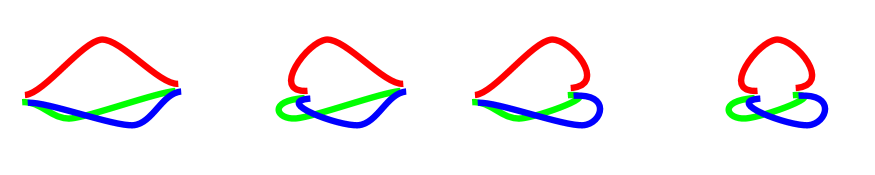
Subsequent moves all make sense for framed bubbles, bizenes, bicrowns and so on. Each gluing move can be done locally in a way which embeds in (embeddings are illustrated in the figures throughout the last few sections); such an embedding determines a move framing on each of the pieces. The difference between a given framing and the move framing determines a class in for each piece, and the sum over all such pieces is the (global) co-orientation cocycle in .
There is a very simple procedure to adjust this global co-orientation cocycle, which we now describe. Suppose we have a pair of footballs and with the same 3 labels, but with framings which differ by a single reflection at a vertex (i.e. they are of the first two types depicted in Figure 9). Swapping and in two cube moves that they participate in adjusts the cocycle six times, once for each of the six edges in the two bubbles; we call this a swap move. If three of these edges are in a component , and three in , then the global change to the cocycle is to add a fundamental class of . If we performed our original gluing randomly, every component should contain many pairs of footballs with framings which differ in this way. So if we take two disjoint copies of , we can trivialize the co-orientation cocycle by finitely many such swaps. This duplication multiplies the total number of components of by a factor of 2.
This completes the proof of the Thin Spine Theorem 3.1.2, at least when .
3.13. Rank 2
The move described in § 3.4 to deal with an excess of long strips requires rank , so that long strips can be grouped into super-compatible 4-tuples if necessary. In this section we briefly explain how to finesse this point in the case .
Fix some constant with ; will need to satisfy some divisibility properties in what follows, but we leave this implicit. Define a pocket to be three equal segments of length which can be glued compatibly. Recall at the very first step of our construction that we glued compatible long strips in triples by bunching sticky segments to form bubbles. We modify this construction slightly by also allowing ourselves to create some small mass of bunched pockets. That is, we bunch triples of long strips of the form
if for even the letters adjacent to each or disagree, where each , or has length , and where each either has length , or has length . We insist that the proportion of of length is very small, so that most of the bunched triples are of length , but that some small mass of bunched pockets has also been created. Note that will depend on the number of “long” , but in any case will be quite close to .
We arrange by pseudorandomness that the mass of bunched pockets of every possible type is , but with a constant such that this mass is definitely larger than the number of long strips that will remain unbunched after the first step.
Now consider a long strip left unbunched after the first step. We partition this strip in a different way as
where each has length , and each has length .
We take 9 copies of . Fix an index . Suppose we have two sets of three bunched triples of pockets (hence 18 pockets in all) of the form
for each of , and satisfying
-
(1)
each of and their primed versions have length ;
-
(2)
each of and their primed versions have length ;
-
(3)
all end with the same letter and all start with the same letter, and similarly for and the primed versions;
-
(4)
end with different letters and start with different letters for each fixed , and similarly for the primed versions;
-
(5)
start with different letters and end with the same letter and similarly for the primed versions;
-
(6)
end with different letters and start with the same letter and similarly for the primed versions;
-
(7)
can be partitioned into an odd number of segments of length which can be compatibly bunched creating a strip of alternate short segments and bubbles, and similarly for the and the primed versions;
-
(8)
the common last letter of the is different from the common last letter of the and from the last letter of , and the common first letter of the is different from the common first letter of the and from the first letter of ; and
-
(9)
, and can be partitioned into an odd number of segments of length which can be compatibly bunched creating a strip of alternate short segments and bubbles.
Under these hypotheses, we can pull apart the six bunched pockets, bunch the in short strips (and similarly bunch the ), bunch the in short strips (and similarly bunch the ), and finally bunch the three sets of , and in short strips. Explicitly, we are creating bunched segments of length of the following kinds:
and finally three copies of
for each of .
If we do this for each in turn, then the net effect is to pair up all the extra long strips, at the cost of creating a new remainder of mass , and using up mass of the bunched pockets.
At the end of this step every vertex of the new remainder created is adjacent to a strip of consecutive short bubbles; because of this, there is ample slack to apply tear moves to the new remainder as in § 3.7. Note that this move requires us to take nine copies of each excess long strip; thus we might have to take a total of 5,832 copies of instead of 648 for . The rest of the argument goes through as above. This completes the proof in the case and thus in general.
4. Bead decomposition
The next step of the argument is modeled very closely on § 5 from [Calegari–Walker(2015)]. For the sake of completeness we explain the argument in detail. Throughout this section we fix a free group with generators and we let be a random cyclically reduced word of length , and consider the one-relator group with presentation complex . Using the Thin Spine Theorem, we will construct (with overwhelming probability) a spine over for which every edge of has length at least , for some big . The main result of this section is that if this construction is done carefully, the immersion will be -injective, again with overwhelming probability.
4.1. Construction of the beaded spine
A random 1-relator group satisfies the small cancellation property for every positive , with overwhelming probability. So to show that is -injective, it suffices to show that for any sufficiently long immersed segment whose image in under lifts to , it already lifts to . Informally, the only long immersed segments in which are “pieces” of are those that are in the image of segments of under .
Let be a 4-valent graph with total edge length , in which every edge has length . For any , there are at most immersed paths in of length . Thus if is of order , and , we would not expect to find any paths of length in common with an independent random relator of length , for any fixed , with probability for some depending on .
There is a nice way to express this in terms of density; or degrees of freedom, which is summarized in the following intersection formula of Gromov; see [Gromov(1993)], § 9.A for details:
Proposition 4.1.1 (Gromov’s intersection formula).
Let be a finite set. For a subset of define the (multiplicative) density of , denoted , to be . If is any subset of , and is a random subset of of fixed cardinality, chosen independently of , then with probability for some , there is an equality
with the convention that means a set is empty.
Note that Gromov does not actually estimate the probability that his formula holds, but this is an elementary consequence of Chernoff’s inequality. For a proof of an analogous estimate, which explicitly covers the cases of interest that we need, see [Calegari–Walker(2013)], § 2.4.
In our situation, taking , we can take to be the set of all reduced words in of length , which has cardinality approximately . If , then the set of immersed paths in of length has density as close to as desired; similarly, the set of subwords of a random word of length has density as close to as desired. Thus if these subwords were independent, Gromov’s formula would show that they were disjoint, with probability .
Of course, the thin spines guaranteed by the Thin Spine Theorem are hardly independent of . Indeed, every subpath of appears in , and therefore in ! Thus, we must work harder to show that these subpaths (those that are already in ) amount to all the intersection. The idea of the bead decomposition is to subdivide into many subsets of length (for some fixed ), to build a thin spine “bounding” the subset , and then to argue that no immersed path in of length can be a piece in any with .
Fix some small positive constant , and write as a product
where each has length and each has length approximately (the exact values are not important, just the order of magnitude). Thus is approximately equal to ; we further adjust the lengths of the and slightly so that is divisible by .
We say a reduced word has small self-overlaps if the length of the biggest proper prefix of equal to a proper suffix is at most . Almost every reduced word of fixed big length has small overlaps. Fix some positive constant , and for each index mod we look for the first triple of subwords of the form in such that
-
(1)
the are single edges;
-
(2)
are distinct and are distinct;
-
(3)
has length with as above; and
-
(4)
has small self-overlaps.
Actually, it is not important that has length exactly ; it would be fine for it to have length in the interval , for example. Any reduced word of length with will appear many times in any random reduced word of length , with probability for some depending on . See e.g. [Calegari–Walker(2013)], §. 2.3. Then for each index mod , the three copies of can be glued to produce unusually long bunched triples that we call lips. The lips partition the remainder of into subsets which we denote , where the index is taken mod , so that each is the union of three segments of length approximately equal to consisting of together with the part of the adjacent outside the lips. We call the beads, and we call the partition of minus the lips into beads the bead decomposition.
Now we apply the Thin Spine Theorem to build a thin spine such that
-
(1)
consists of 648 copies of (or 5,832 copies if );
-
(2)
is cyclically subdivided by the lips into connected subgraphs ;
-
(3)
the 648 copies of in are precisely the part of mapping to the , and the remainder of consists of segments mapping to the lips as above.
We call the result a beaded spine.
Lemma 4.1.2 (No common path).
For any positive , we can construct a beaded spine with the property that no immersed path in of length can be a piece in any with mod , with probability , where depends on .
Proof.
The construction of a beaded spine is easy: with high probability, the labels on each are -pseudorandom for any fixed , and we can simply apply the construction in the Thin Spine Theorem to each individually to build , and correct the co-orientation once at the end by a local modification in (say).
By the nature of the bead decomposition, the are independent of each other. By thinness, there are immersed paths in of length . For any fixed positive , if we set , and choose big enough, then the density of this set of paths (in the set of all reduced words of length ) is as close to as we like. Similarly, the set of subwords in of length has density as close to as we like for big . But now these subwords are independent of the immersed paths in , so by the intersection formula (Proposition 4.1.1), there are no such words in common, with probability . ∎
4.2. Injectivity
We now show why a beaded spine gives rise to a -injective map of a 3-manifold . First we prove another lemma, which is really the key geometric point, and will be used again in § 6:
Lemma 4.2.1 (Common path lifts).
For any positive , with probability we can construct a beaded spine with the property that any immersed segment with whose image in under lifts to or , already lifts to .
In words, this lemma says that any path in of length which immerses in lifts to , and therefore appears in the boundary of a disk of .
Proof.
The proof follows very closely the proof of Lemma 5.2.3 from [Calegari–Walker(2015)].
First, fix some very small with where is the length of the lips in the beaded spine. This ensures that a random word of length is very unlikely to contain two copies of any word of length with small self-overlaps; see e.g. [Calegari–Walker(2013)] Prop. 2.6 and Prop. 2.11 which says that the likelihood of this occurrence is for some .
Now, let be an immersed path of length whose label is a subpath of or ; this means that there is another immersion such that the compositions and agree.
Using , we decompose into subpaths which are the preimages of the segments of under . Apart from boundary terms, each of these has length approximately . By Lemma 4.1.2, no can immerse in with mod unless , and in fact must therefore take all of into except possibly for some peripheral subwords of length at most .
But this means that for all , there is a subpath centered at the common endpoint of and , with , for which one endpoint maps under into and the other into . This means that must map over the lip of separating from , and must contain a copy of the word on that lip. But under the map , the word contains another copy of . By our hypothesis on , the probability that contains two copies of is . If these copies are the same, then the composition and agree on . But since is an immersion, it follows that and must agree on all of ; i.e. that lifts to , as claimed.
So the lemma is proved unless there are two distinct copies of within distance of each lip in the image of . Since has length , there are such lips; the probability of two distinct copies for each lip is , and the probabilities for distinct lips are independent, so the total probability is and we are done. ∎
An immediate corollary is the existence of 3-manifold subgroups in random 1-relator groups:
Proposition 4.2.2.
Let be a random 1-relator group where . Then with probability we can produce a beaded spine for which the associated map is -injective.
Proof.
Suppose not, so that there is an immersed loop which is nontrivial in , but trivial in . There is a van Kampen diagram with boundary . If is a disk in this diagram with some segment in common with , and if lifts to , then bounds a disk in , and we can push across by a homotopy, producing a diagram with fewer disks. A diagram which does not admit such a simplification is said to be efficient; without loss of generality therefore we obtain an efficient diagram whose boundary is an immersed loop .
The group satisfies the small cancellation property for any positive . Thus by Greedlinger’s Lemma, if we take small enough, some disk in the diagram has a segment of its boundary of length at least in common with . Note that is labeled or , and has length . Since as in Lemma 4.2.1, the boundary of this path actually lifts to , whence the diagram is not efficient after all. This contradiction proves the theorem. ∎
Note that each boundary component of is of the form for some 3-valent fatgraph immersed in ; thus the same argument implies that every component of is -injective, and therefore has incompressible boundary. Furthermore, since is aspherical, so is , and therefore is irreducible, and does not split as a free product.
To show that is homotopic to a hyperbolic 3-manifold with totally geodesic boundary, it suffices to show that it is acylindrical, by Thurston’s hyperbolization theorem—see, for instance, [Bonahon(2002), Theorem 4.3]. We show this in § 5.
5. Acylindricity
In this section we explain why the 3-manifolds we have produced in random 1-relator groups are acylindrical.
Theorem 5.0.1 (1-Relator Acylindrical Subgroup Theorem).
Let be a random 1-relator group where . Then with probability for the beaded spine guaranteed by Proposition 4.2.2 the 3-manifold is acylindrical. Thus, with overwhelming probability, random 1-relator groups contain subgroups isomorphic to the fundamental group of a hyperbolic 3-manifold with totally geodesic boundary.
Proof.
Each boundary component is of the form for some trivalent fatgraph immersed in . Suppose admits an essential annulus. Then there is a van Kampen diagram on an annulus with boundary where immerses in for fatgraphs associated to boundary components as above, and each is essential in (which in turn is essential in ).
Assume that is efficient. Then by Lemma 4.2.1, for any positive we can insist that no segment of has length more than . For big , with probability we know that is for any positive ; when is small, the annular version of Greedlinger’s Lemma (see [Lyndon–Schupp(1977)] Ch. V Thm. 5.4 and its proof) implies that if contains a disk at all, then some disk in the diagram has a segment on its boundary of length at least in common with or . Taking we see that can contain no disks at all; i.e. and have the same image in .
Now we use the fact that is a good spine. At each vertex of , four local boundary components of meet; the fact that lifts to paths and in two of these component forces to run between two specific edges incident to , and this determines a unique lift of to near compatible with the existence of the . Similarly, along each edge of , three local boundary components of meet; the components containing and thus again determine a unique lift of to along . These local lifts at vertices and along edges are compatible, and determine a global lift of to . But this means is inessential in , contrary to hypothesis. Thus is acylindrical after all. ∎
6. 3-Manifolds Everywhere
We now show that the acylindrical 3-manifold subgroups that we have constructed in random 1-relator groups stay essential as we add independent random relations of length , for any . Our argument follows the proof of Thm. 6.4.1 [Calegari–Walker(2015)] exactly, and depends only on the following two facts:
-
(1)
the beaded spine has total length , has valence 4, and every segment has length at least , where we may choose as big as we like (depending on ); and
-
(2)
any immersed segment of length whose label is a subword of or lifts to , where we may choose as small as we like (depending on ).
Beyond these facts, we use two theorems of [Ollivier(2007)], which give explicit estimates for the linear constant in the isoperimetric function and for the constant of hyperbolicity for a random group at density .
6.1. Ollivier’s estimates
We use the following theorems of [Ollivier(2007)]:
Theorem 6.1.1 ([Ollivier(2007)], Thm. 2).
Let be a random group at density . Then for any positive , and any efficient van Kampen diagram containing disks, we have
with probability .
Theorem 6.1.2 ([Ollivier(2007)], Cor. 3).
Let be a random group at density . Then the hyperbolicity constant of the presentation satisfies
with probability .
From this, we will deduce the following lemma, which is the exact analog of [Calegari–Walker(2015)] Lem. 6.3.2, and is deduced in exactly the same way from Ollivier’s theorems:
Lemma 6.1.3.
Let be a 3-manifold obtained from a beaded spine, and suppose it is not -injective in , a random group at density . Then there are constant and depending only on , a geodesic path in of length at most , and a van Kampen diagram containing at most faces so that and .
Proof.
Theorem 6.1.2 says that , and in any -hyperbolic geodesic metric space, a -local geodesic is a (global) -quasigeodesic for any (see [Bridson–Haefliger(1999)], Ch. III. H, 1.13 p. 405). A local geodesic in the 1-skeleton of corresponding to an element of the kernel must contain a subsegment of length at most which is not a local geodesic in . The lift of this subsegment to the universal cover (i.e. the Cayley complex of ) cobounds a van Kampen diagram with an honest geodesic segment in . But by Theorem 6.1.1, the diagram must satisfy
where is the number of faces; thus is bounded in terms of , and independent of . ∎
6.2. Proof of the main theorem
Theorem 6.2.1 (3-Manifolds Everywhere).
Fix . A random -generator group — either in the few relators model with relators, or the density model with density — with relators of length contains many quasi-isometrically embedded subgroups isomorphic to the fundamental group of a hyperbolic 3-manifold with totally geodesic boundary, with probability for some .
Proof.
The proof exactly follows the proof of Thm. 6.4.1 from [Calegari–Walker(2015)]. Pick one relation and build and by the method of § 3. We have already seen that is homotopy equivalent to a hyperbolic 3-manifold with totally geodesic boundary, and that its fundamental group injects into ; we now show that it stays injective in when we add another independent random relations of length .
The argument is a straightforward application of Gromov’s intersection formula, i.e. Proposition 4.1.1. It is convenient to express it in terms of degrees of freedom, measured multiplicatively as powers of . Suppose is not -injective. Then by Lemma 6.1.3 there is an efficient van Kampen diagram with faces (where depends only on ), and a local geodesic which immerses in with and . The choice of gives degrees of freedom, where and where , since there are immersed paths in of length , and we have . Taking as big as necessary, we can make as small as we like.
Next, disks in with boundary label or cannot have segments of length more than in common either with themselves or with in an efficient van Kampen diagram, where as in Lemma 4.2.1 can be taken as small as we like. Since there are at most disks in , two distinct disks cannot have more than boundary segments in common. Take small enough so that . Then if we let denote the result of cutting the disks labeled or out of the diagram, and let denote the union
and the number of disks in , then we have inequalities , and with equality if and only if .
Each remaining choice of face gives degrees of freedom, and each segment in the interior of length imposes degrees of constraint. Similarly, itself imposes degrees of constraint. Let denote the union of interior edges. Then so because . On the other hand, the total degrees of freedom is if is small enough, so there is no way to assign labels to the faces to build a compatible diagram, with probability . There are polynomial in ways to assign lengths to the edges, and a finite number of possible combinatorial diagrams (since each diagram has at most disks); summing the exceptional cases over all such diagrams shows that the probability of finding some such diagram is . Otherwise is -injective, as claimed.
Finally, we prove that is quasi-isometrically embedded in . Indeed, as observed already in [Calegari–Walker(2015)], the above argument actually shows that for any we can construct for which is quasi-isometrically embedded in . Controlling depends only on applying the argument above to segments of length at most for suitable . The constant then bounds the number of disks in an efficient van Kampen diagram, by Theorem 6.1.1. ∎
7. Commensurability
Once we know that random groups contain many interesting 3-manifold subgroups, it is natural to wonder exactly which 3-manifold groups arise. For any fixed non-free finitely presented group , there are no injective homomorphisms from to a random group at fixed density once the relators in get sufficiently long (with overwhelming probability). So it is probably hopeless to try to understand precisely which subgroups arise, since this will depend in a very complicated way on the length of the relators. However, we are in better shape if we simply try to control the commensurability class of the subgroups.
Example 7.0.1.
There are 24 simplices in the barycentric subdivision of a regular Euclidean tetrahedron. Three edges of this simplex have dihedral angles , two have dihedral angles , and one (the edge lying on the edge of the original simplex) has a dihedral angle of the form , which is approximately . If we deform the dihedral angle of this last edge while keeping the other dihedral angles fixed, the simplex admits a unique hyperbolic metric for all at which point one vertex of the simplex becomes ideal. If we try to deform to , then three of the faces of the simplex don’t meet at all, and there is a perpendicular plane which intersects these three faces in the edges of a hyperbolic triangle with angles . If is of the form for some integer , the group generated by reflections in the 4 sides of the (now-infinite) hyperbolic polyhedron is discrete, and convex cocompact. This group is a Coxeter group which we denote , and whose Coxeter diagram is
The groups with are finite. The group is commensurable with the fundamental group of the figure 8 knot complement. For any the limit set of is a (round) Sierpinski carpet. Figure 10 depicts a simply-connected 2-complex stabilized by with cocompact fundamental domain which is a “dual” spine to the (infinite) polyhedron described above. The faces of this 2-complex are regular 7-gons, and the vertices are all 4-valent with tetrahedral symmetry.
2pt
\endlabellist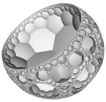
As , the limit sets converge to the Apollonian gasket, which has Hausdorff dimension about . The convex covolumes of — i.e. the volumes of the convex hulls of — are uniformly bounded above independently of .
We now observe that we can arrange for the 3-manifold groups we construct to be commensurable with some .
Theorem 7.0.2 (Commensurability Theorem).
A random group at any density or in the few relators model contains (with overwhelming probability) a subgroup commensurable with the Coxeter group for some , where is the Coxeter group with Coxeter diagram
Proof.
The group acts cocompactly on a simply-connected 2-dimensional complex in whose faces are totally geodesic regular hyperbolic -gons, and whose vertices are 4-valent and are stabilized by a tetrahedral symmetry group; the case is depicted in Figure 10. So to prove the theorem it suffices to show that we can build our thin spines in such a way that each component of maps over exactly edges of the 4-valent graph . But this is elementary to arrange: the only point in the construction in which the number of edges of the components of might vary is during the operations of super-compatible gluing, the adjustments in § 3.6, and trades. In each of these cases all that is relevant is the types of pieces being glued or traded, and not which components of are involved. Since types of the desired kind for each move can be found on any component, we can simply distribute the moves evenly over the different components, possibly after taking multiple copies of to clear denominators. The proof immediately follows ∎
There is nothing very special about the commensurability classes , except that their fundamental domains are so small, so that their local combinatorics are very easy to describe.
Definition 7.0.3.
A geodesic spine is a finite 2-dimensional complex with totally geodesic edges and faces which embeds in some hyperbolic 3-manifold with totally geodesic boundary as a deformation retract. We say that a 2-dimensional orbifold complex is obtained by orbifolding if its underlying complex is homeomorphic to , and it is obtained by adding at most one orbifold point to each face of . Note that each such has an (orbifold) fundamental group which is commensurable with an acylindrical 3-manifold group.
In view of the level of control we are able to impose on the combinatorial type of the thin spines we construct in § 3, we make the following conjecture:
Conjecture 7.0.4.
For any fixed geodesic spine , a random group — either in the few relators model or the density model with density — contains subgroups commensurable with the (orbifold) fundamental group of some orbifolding of (with overwhelming probability).
8. Acknowledgments
Danny Calegari was supported by NSF grant DMS 1005246. Henry Wilton was supported by an EPSRC Career Acceleration Fellowship. We would like to thank François Dahmani for raising the main question addressed by this paper, and for his continued interest. We would also like to thank Pierre de la Harpe for comments and corrections.
References
- [Agol(2013)] I. Agol (with an appendix with D. Groves and J. Manning), The virtual Haken conjecture, Doc. Math. 18 (2013), 1045–1087
- [Bonahon(2002)] F. Bonahon Geometric structures on 3-manifolds, Handbook of geometric topology, North-Holland, Amsterdam, 2002, 93–164
- [Bowditch(1998)] B. Bowditch, Cut points and canonical splittings of hyperbolic groups, Acta Math. 180 (1998), no. 2, 145–186
- [Bridson–Haefliger(1999)] M. Bridson and A. Haefliger, Metric spaces of nonpositive curvature, Grund. der math. Wiss. Springer-Verlag Berlin 1999
- [Calegari–Walker(2013)] D. Calegari and A. Walker, Random rigidity in the free group, Geom. Topol. 17 (2013), 1707–1744
- [Calegari–Walker(2015)] D. Calegari and A. Walker, Random groups contain surface subgroups, Jour. AMS 28 (2015), no. 2, 383–419
- [Dahmani–Guirardel–Przytycki(2011)] F. Dahmani, V. Guirardel, and P. Przytycki. Random groups do not split, Math. Ann. 249 (2011), no. 3, 657–673
- [Gromov(1993)] M. Gromov, Asymptotic invariants of infinite groups, Geometric group theory, vol. 2; LMS Lecture Notes 182 (Niblo and Roller eds.) Cambridge University Press, Cambridge, 1993
- [Kahn–Markovic(2011)] J. Kahn and V. Markovic, The good pants homology and a proof of the Ehrenpreis conjecture, preprint, arXiv:1101.1330
- [Kapovich–Kleiner(2000)] M. Kapovich and B. Kleiner, Hyperbolic groups with low dimensional boundary, Ann. Sci. École Norm. Sup. (4) 33 (2000), no. 5, 647–669
- [Keevash(2014)] P. Keevash, The existence of designs, preprint, arXiv:1401.3665
- [Lyndon–Schupp(1977)] R. Lyndon and P. Schupp, Combinatorial group theory, Ergeb. der Math. und ihr. Grenz. 89, Springer-Verlag, Berlin-New York, 1977
- [Ollivier(2007)] Y. Ollivier, Some small cancellation properties of random groups, Internat. J. Algebra Comput. 17 (2007), no. 1, 37–51
- [Stallings(1968)] J. Stallings, On torsion-free groups with infinitely many ends, Ann. Math. 88 (1968), 312–334
- [Stallings(1983)] J. Stallings, Topology of finite graphs, Invent. Math. 71 (1983), no. 3, 551–565