This paper was converted on www.awesomepapers.org from LaTeX by an anonymous user.
Want to know more? Visit the Converter page.

6D Radar Sensing and Tracking in Monostatic Integrated Sensing and Communications System

Hongliang Luo, Feifei Gao, Fan Liu and Shi Jin H. Luo and F. Gao are with Department of Automation, Tsinghua University, Beijing 100084, China (email: luohl23@mails.tsinghua.edu.cn; feifeigao@ieee.org).F. Liu is with the Department of Electrical and Electronic Engineering, Southern University of Science and Technology, Shenzhen 518055, China (e-mail: liuf6@sustech.edu.cn).S. Jin is with the National Mobile Communications Research Laboratory, Southeast University, Nanjing 210096, China (e-mail: jinshi@seu.edu.cn).
Abstract

In this paper, we propose a novel scheme for six-dimensional (6D) radar sensing and tracking of dynamic target based on multiple input and multiple output (MIMO) array for monostatic integrated sensing and communications (ISAC) system. Unlike most existing ISAC studies believing that only the radial velocity of far-field dynamic target can be measured based on one single base station (BS), we find that the sensing echo channel of MIMO-ISAC system actually includes the distance, horizontal angle, pitch angle, radial velocity, horizontal angular velocity, and pitch angular velocity of the dynamic target. Thus we may fully rely on one single BS to estimate the dynamic target’s 6D motion parameters from the sensing echo signals. Specifically, we first propose the long-term motion and short-term motion model of dynamic target, in which the short-term motion model serves the single-shot sensing of dynamic target, while the long-term motion model serves multiple-shots tracking of dynamic target. As a step further, we derive the sensing channel model corresponding to the short-term motion. Next, for single-shot sensing, we employ the array signal processing methods to estimate the dynamic target’s horizontal angle, pitch angle, distance, and virtual velocity. By realizing that the virtual velocities observed by different antennas are different, we adopt plane fitting to estimate the radial velocity, horizontal angular velocity, and pitch angular velocity of dynamic target. Furthermore, we implement the multiple-shots tracking of dynamic target based on each single-shot sensing results and Kalman filtering. Simulation results demonstrate the effectiveness of the proposed 6D radar sensing and tracking scheme.

Index Terms:
6D MIMO radar, angular velocity estimation, integrated sensing and communications, dynamic target sensing, dynamic target tracking.

I Introduction

In the past decade, the integration of wireless communications and radar sensing has promoted the researches on dual functions radar communications (DFRC) systems[1, 2]. With the further expansion of the connotation and extension of sensing, integrated sensing and communications (ISAC) that incorporates more diverse sensing technologies based on DFRC has been recognized as a promising air-interface technology for next-generation wireless networks[3, 4, 5]. Since ISAC allows sensing systems and communications systems to share spectrum resources, and can serve various intelligent applications, it has also been officially approved by ITU-R IMT 2030 as one of the six key usage scenarios for the sixth generation (6G) mobile communications[6, 7].

The ultimate functionality of sensing is to construct the mapping relationship from real physical world to digital twin world, where the former includes static environment (such as roads and buildings) and dynamic targets (such as pedestrians and vehicles). Therefore, realizing static environment reconstruction and dynamic target sensing is becoming one consensus among researchers. Specifically, dynamic target sensing, as a research focus, refers to the discovery, detection, parameters estimation, tracking, and recognition of target based on the radar sensing function of ISAC system.

On the other side, the base stations (BSs) in ISAC systems are usually stationary and are configured with massive multiple input and multiple output (MIMO) arrays. Depending on the number and location of BSs, the ISAC system can be divided into: 1) monostatic ISAC system (only one BS in the system); 2) bistatic ISAC system (two BSs in the system); and 3) multistatic ISAC system (multiple BSs in the system)[8, 9]. Among different ISAC architectures, monostatic ISAC system has received tremendous research attention due to low implementation complexity, as it does not require high-precision synchronization among BSs.

More relevant to this work, estimating the motion parameters of dynamic target with monostatic ISAC system has been well-investigated in the past few years. For example, X. Chen et. al. proposed a multiple signal classification based monostatic ISAC system that can attain high accuracy for target’s angle, distance, and radial velocity estimation[10]. W. Jiang et. al. proposed a model-driven ISAC scheme, which simultaneously accomplished tasks of demodulating uplink communications signals and estimating distance and radial velocity of dynamic target[11]. In order to track dynamic target, F. Liu et. al. investigated a sensing assisted predictive beamforming design for vehicle communications by exploiting ISAC technique[12]. On top of that, Z. Du et. al. proposed a tracking scheme for extended target based on extended Kalman filtering and beamwidth adjustment, which leveraged matched filtering and maximum likelihood estimation to obtain the angle, distance, and radial velocity of target, and then tracks the target[13]. It should be noted that all of these works adopt the traditional view in the field of radar sensing that only the radial velocity of dynamic target can be measured based on one single BS, while the angular velocity cannot be directly measured. Even in the field of radar sensing, the most advanced researches currently available suggest that the monostatic MIMO radar can and only can realize the 4D sensing of dynamic target, namely, measuring the dynamic target’s horizontal angle, pitch angle, distance, and radial velocity[14, 15]. However, by re-examining the relationship between the motion parameters of dynamic target and the sensing echo channel of MIMO system, one may realize that the sensing channel already encompasses the distance, horizontal angle, pitch angle, radial velocity, horizontal angular velocity, and pitch angular velocity of the dynamic target. As a consequence, it becomes possible to estimate the dynamic target’s 6D motion parameters from the echo signals based on one single BS.

Evidently, there are already some preliminary studies focusing on measuring the angular velocity based on monostatic radar system. J. A. Nanzer et. al. first proposed the theoretical method for measuring the angular velocity of moving object based on spatial interferometry using one single station radar system, which was later verified through hardware experiments[16, 17, 18, 19]. X. Wang et. al. extended this work to multiple targets angular velocities measurement scenarios through conceiving sophisticated algorithms[20, 21, 22]. However, all of these studies only considered the spatial interference effect between two or three antennas, resulting in severe sensing performance loss. To the best knowledge of the authors, estimating the angular velocity based on single station massive MIMO-OFDM system still remains widely unexplored.

In this paper, we attempt to fill in this research gap by proposing a novel scheme for 6D radar single-shot sensing and multiple-shots tracking of dynamic target based on massive MIMO array for monostatic ISAC system. The contributions of this paper are summarized as follows.

  • Based on the working pipeline of radar sensing in ISAC system, we construct the long-term motion and short-term motion model for dynamic target in 3D space, which correspond to multiple-shots tracking and single-shot sensing of dynamic target, respectively.

  • We re-examine the relationship between the 6D motion parameters of dynamic target and the sensing echo channel of MIMO-ISAC system, and reveal that the sensing channel actually includes the distance, horizontal angle, pitch angle, radial velocity, horizontal angular velocity, and pitch angular velocity of target, which enables us to estimate the dynamic target’s 6D motion parameters from echoes by solely relying on one single ISAC BS.

  • For single-shot sensing, we employ the array signal processing methods to estimate the dynamic target’s distance, horizontal angle, pitch angle, and virtual velocity. Then we show that the virtual velocities observed at different antennas are distinct from each other, allowing us to utilize plane fitting to estimate the radial velocity, horizontal angular velocity, and pitch angular velocity of the dynamic target.

  • Based on the single-shot 6D parameters sensing results, we further propose a multiple-shots tracking approach for dynamic target through Kalman filtering.

The remainder of this paper is organized as follows. In Section II, we propose the 6D motion model of dynamic target, and derive the corresponding sensing channel model. In Section III, we propose a novel 6D sensing and tracking scheme for dynamic target sensing. Simulation results and conclusions are given in Section IV and Section V, respectively.

Notation: Lower-case and upper-case boldface letters 𝐚\mathbf{a} and 𝐀\mathbf{A} denote a vector and a matrix; 𝐚T\mathbf{a}^{T} and 𝐚H\mathbf{a}^{H} denote the transpose and the conjugate transpose of vector 𝐚\mathbf{a}, respectively; [𝐚]n[\mathbf{a}]_{n} denotes the nn-th element of the vector 𝐚\mathbf{a}; [𝐀]i,j[\mathbf{A}]_{i,j} denotes the (i,j)(i,j)-th element of the matrix 𝐀\mathbf{A}; 𝐀[i1:i2,:]\mathbf{A}[i_{1}:i_{2},:] is the submatrix composed of all columns elements in rows i1i_{1} to i2i_{2} of matrix 𝐀\mathbf{A}; 𝐀[:,j1:j2]\mathbf{A}[:,j_{1}:j_{2}] is the submatrix composed of all rows elements in columns j1j_{1} to j2j_{2} of matrix 𝐀\mathbf{A}; eig(){\rm eig}(\cdot) represents the matrix eigenvalue decomposition function.

II System Model and Proposed ISAC Framework

In this section, we provide the generic model for massive MIMO based monostatic ISAC system, and propose the 6D motion model of dynamic target, as well as derive the sensing channel model of ISAC system.

II-A ISAC BS Model

Refer to caption
Figure 1: System model.

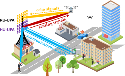
A massive MIMO based monostatic ISAC system operating in mmWave or Terahertz frequency bands with OFDM modulation is depicted in Fig. 1, which employs only one dual-functional BS for wireless communications and radar sensing at the same time. Generally, we consider that the BS consists of one hybrid unit (HU) and one radar unit (RU), where both the HU and the RU are configured with uniform planar arrays (UPAs). By designing the beamforming strategy, HU is responsible for transmitting downlink communications signals and receiving uplink communications signals, as well as transmitting downlink sensing signals to realize dynamic target sensing; while RU is responsible for receiving echo signals to realize dynamic target sensing.

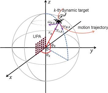
The HU and RU are each equipped with one UPA of NH=NHx×NHzN_{H}=N^{x}_{H}\times N_{H}^{z} and NR=NRx×NRzN_{R}=N_{R}^{x}\times N_{R}^{z} antenna elements, named as HU-UPA and RU-UPA, respectively. Assume that both the HU-UPA and the RU-UPA are vertically mounted on the 2D plane y=0y=0 at BS side as shown in Fig. 2, and the antenna spacing between the antennas distributed along x-axis and z-axis are dx=dλ2d_{x}=d\leq\frac{\lambda}{2} and dz=dλ2d_{z}=d\leq\frac{\lambda}{2}, respectively, with λ\lambda being the wavelength. Without loss of generality, we denote the position of the nHn_{H}-th antenna element in the HU-UPA as 𝐩nH=𝐩0H+[dnHx,0,dnHz]T\mathbf{p}_{n_{H}}=\mathbf{p}_{0_{H}}+[d\cdot n_{H}^{x},0,d\cdot n_{H}^{z}]^{T}, where 𝐩0H\mathbf{p}_{0_{H}} is the position of the reference element, nHx{0,1,,NHx1}n_{H}^{x}\in\{0,1,...,N_{H}^{x}-1\} and nHz{0,1,,NHz1}n_{H}^{z}\in\{0,1,...,N_{H}^{z}-1\} are the antenna indices. Here we use two types of index numbers to represent the same antenna, that is, the nHn_{H}-th antenna may also be named as the (nHx,nHz)(n^{x}_{H},n^{z}_{H})-th antenna. Similarly, we denote the position of the nRn_{R}-th antenna element in the RU-UPA as 𝐩nR=𝐩0R+[dnRx,0,dnRz]T\mathbf{p}_{n_{R}}=\mathbf{p}_{0_{R}}+[d\cdot n_{R}^{x},0,d\cdot n_{R}^{z}]^{T} with nRx{0,1,,NRx1}n_{R}^{x}\in\{0,1,...,N^{x}_{R}-1\} and nRz{0,1,,NRz1}n_{R}^{z}\in\{0,1,...,N^{z}_{R}-1\}. Generally, according to the spatial consistency of the arrays, we further assume that the HU-UPA and RU-UPA are co-located and are parallel to each other, i.e., 𝐩0H=𝐩0R=[0,0,0]T\mathbf{p}_{0_{H}}=\mathbf{p}_{0_{R}}=[0,0,0]^{T}, such that they may see the targets at the same propagation directions111Since the normal communications and sensing distance is much longer than the protection distance between HU-UPA and RU-UPA, it can be considered that HU-UPA and RU-UPA are located in the same position.[23]. Besides, by balancing the hardware costs and system performance, we assume that the HU-UPA employs the hardware architecture based on phase shifter (PS) structure, in which a total of NH,RFNHN_{H,RF}\ll N_{H} radio frequency (RF) chains are deployed, and each antenna is connected to a PS to realize beamforming. On the other side, we assume that the RU-UPA employs the fully-digital receiving array, with each antenna connected to one RF chain, to realize super-resolution sensing performance, which follows the setting in [10] and [23].

Refer to caption
Figure 2: BS model and dynamic target motion parameters.
Refer to caption
Figure 3: The proposed ISAC framework.

Suppose that the ISAC system emits OFDM signals with MM subcarriers, where the lowest frequency and the subcarrier interval of OFDM signals are f0f_{0} and Δf\Delta f, respectively. Then the transmission bandwidth is W=(M1)ΔfW=(M-1)\Delta f, and the frequency of the mm-th subcarrier is fm=f0+mΔff_{m}=f_{0}+m\Delta f, where m=0,1,,M1m=0,1,...,M-1. Further, we consider that an OFDM frame contains NN consecutive OFDM symbols, where the time interval between adjacent OFDM symbols is Ts=Ts+TgT_{s}=T^{\prime}_{s}+T_{g}, with Ts=1ΔfT^{\prime}_{s}=\frac{1}{\Delta f} and TgT_{g} being the OFDM symbol duration and guard interval, respectively.

We employ the spherical coordinates (r,θ,ϕ)(r,\theta,\phi) to represent one position in 3D space. As shown in Fig. 2, rr represents the polar distance with mathematical range of r0r\geq 0, θ\theta represents the horizontal angle with mathematical range of 0θ1800^{\circ}\leq\theta\leq 180^{\circ}, and ϕ\phi represents the pitch angle with mathematical range of 90ϕ90-90^{\circ}\leq\phi\leq 90^{\circ}. Moreover, the spherical coordinate (r,θ,ϕ)(r,\theta,\phi) may be translated to its Cartesian counterpart (x,y,z)(x,y,z) through

x=rcosϕcosθ,y=rcosϕsinθ,z=rsinϕ.\displaystyle x=r\cos\phi\cos\theta,\quad y=r\cos\phi\sin\theta,\quad z=r\sin\phi. (1)

Since BS is located at the origin of coordinate system, we denote the service area of BS as {(r,θ,ϕ)|rminrrmax,θminθθmax,ϕminϕϕmax}\{(r,\theta,\phi)|r_{min}\leq r\leq r_{max},\theta_{min}\leq\theta\leq\theta_{max},\phi_{min}\leq\phi\leq\phi_{max}\}. Suppose that there are PP single-antenna communications users, KK dynamic targets, as well as widely distributed static environment within this service area. We assume that the 6D motion parameters of the kk-th dynamic target are {rk,θk,ϕk,vr,k,ωθ,k,ωϕ,k}\{r_{k},\theta_{k},\phi_{k},v_{r,k},\omega_{\theta,k},\omega_{\phi,k}\}, in which (rk,θk,ϕk)(r_{k},\theta_{k},\phi_{k}) represents the position of the kk-th target, vr,kv_{r,k}, ωθ,k\omega_{\theta,k} and ωϕ,k\omega_{\phi,k} represent the radial velocity, horizontal angular velocity, and pitch angular velocity, respectively. Besides, we assume that the position of the pp-th user is (Rp,ϑp,φp)(R_{p},\vartheta_{p},\varphi_{p}), which are known and stationary to BS, due to the fact that they can be easily obtained through user reporting, or other techniques[24, 25, 26].

II-B The Proposed ISAC Framework

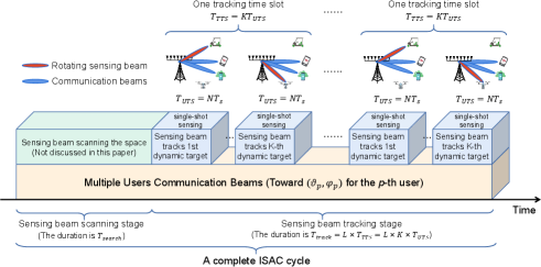
The task of ISAC system is to sense all KK dynamic targets while serving the communications of all PP users. As described in Fig. 3, the proposed ISAC framework consists of two stages: sensing beam scanning (SBS) stage and sensing beam tracking (SBT) stage. For the aspect of communications, BS continuously generates PP communications beams towards PP users to maintain communications service during both SBS stage and SBT stage. For the aspect of sensing, BS generates one sensing beam that can scan the service area during SBS stage, during which the BS may detect the targets and estimate their parameters. To proceed, BS generates a single sensing beam to track all KK dynamic targets in a time division manner during SBT stage, that is, the sensing beam may sequentially illuminate each target and continuously track them. In this work, we mainly focuses on the SBT stage, and refer readers to our previous work [27] for more details on the SBS stage.

Assume that KK dynamic targets possess different physical directions. At each direction, the BS may adopt one OFDM frame, i.e., NN consecutive OFDM symbols, to realize dynamic target sensing. As shown in Fig. 3, we divide the SBT stage into LL tracking time slots (TTSs), and each TTS lasts for a time duration of TTTS=KNTsT_{TTS}=K\cdot N\cdot T_{s}. Besides, each TTS is further divided into KK unit time slots (UTSs), and each UTS lasts for a time duration of TUTS=NTsT_{UTS}=N\cdot T_{s}. Clearly, there is TTTS=KTUTST_{TTS}=K\cdot T_{UTS}. During LL consecutive TTSs, BS should track all KK dynamic targets using the methods such as Kalman filtering with TTTST_{TTS} as time step, which is named as multiple-shots tracking. To realize continuous target tracking and reliable users communications, in the (l,k)(l,k^{\prime})-th UTS, BS needs to generate PP communications beams pointing to PP users and generate one sensing beam pointing to the sensing tracking direction (ξlk,ηlk)(\xi_{lk^{\prime}},\eta_{lk^{\prime}}) from HU-UPA, where k=1,2,,Kk^{\prime}=1,2,...,K. The BS needs to update the motion parameter sensing results of the kk^{\prime}-th dynamic target within this UTS, known as single-shot sensing. Ideally, (ξlk,ηlk)(\xi_{lk^{\prime}},\eta_{lk^{\prime}}) should be equal to the physical direction of the kk^{\prime}-th dynamic target in the (l,k)(l,k^{\prime})-th UTS.

Here we assume that the transmission power of BS is PtP_{t}, the energy of sensing beam is ρlkPt\rho_{lk^{\prime}}P_{t}, and the remaining energy (1ρlk)Pt(1-\rho_{lk^{\prime}})P_{t} is evenly distributed among communications beams, where ρlk[0,1]\rho_{lk^{\prime}}\in[0,1] is the power distribution coefficient used in the (l,k)(l,k^{\prime})-th UTS. Due to the short duration of one UTS, we keep the directions of transmitting beams unchanged within one UTS. Then the transmission signals from HU-UPA on the mm-th subcarrier of the nn-th symbol in the (l,k)(l,k^{\prime})-th UTS should be represented as

𝐱lk,n,m=p=1P𝐰c,p,lksn,mc,p,lk+𝐰s,lksn,ms,lk=p=1P(1ρlk)PtPNH𝐚H(Γp,Υp)sn,mc,p,lk+ρlkPtNH𝐚H(Ξlk,Θlk)sn,ms,lk,\begin{split}\begin{aligned} \!\!\!&\mathbf{x}_{lk^{\prime}\!,n,m}=\sum_{p=1}^{P}\mathbf{w}_{c,p,lk^{\prime}}s^{c,p,lk^{\prime}}_{n,m}+\mathbf{w}_{s,lk^{\prime}}s^{s,lk^{\prime}}_{n,m}\\ &\!\!\!=\!\!\!\sum_{p=1}^{P}\!\!\!\sqrt{\!\!\frac{(\!1\!\!-\!\!\rho_{lk^{\prime}})\!P_{\!t}}{PN_{H}}}\!\mathbf{a}_{\!H}\!(\Gamma_{p}\!,\!\!\Upsilon_{p}\!)\!s^{c,p,lk^{\prime}}_{n,m}\!\!\!\!+\!\!\!\sqrt{\!\frac{\rho_{lk^{\prime}}\!P_{\!t}}{N_{H}}}\!\mathbf{a}_{\!H}\!(\Xi_{lk^{\prime}}\!,\!\Theta_{lk^{\prime}}\!)\!s^{s,lk^{\prime}}_{n,m}\!,\end{aligned}\end{split} (2)

where (Γp,Υp)=(cosφpcosϑp,sinφp)(\Gamma_{p},\Upsilon_{p})\!=\!(\cos\varphi_{p}\cos\vartheta_{p},\sin\varphi_{p}) is the spatial-domain direction corresponding to the physical direction (ϑp,φp)(\vartheta_{p},\varphi_{p}) of the pp-th user, and (Ξlk,Θlk)=(cosηlkcosξlk,sinηlk)(\Xi_{lk^{\prime}},\Theta_{lk^{\prime}})=(\cos\eta_{lk^{\prime}}\cos\xi_{lk^{\prime}},\sin\eta_{lk^{\prime}}) is the spatial-domain direction corresponding to the sensing tracking direction (ξlk,ηlk)(\xi_{lk^{\prime}},\eta_{lk^{\prime}}). Besides, 𝐰c,p,lk=(1ρlk)PtPNH𝐚H(Γp,Υp)\mathbf{w}_{c,p,lk^{\prime}}=\sqrt{\frac{(1-\rho_{lk^{\prime}})P_{t}}{PN_{H}}}\mathbf{a}_{H}(\Gamma_{p},\Upsilon_{p}) and 𝐰s,lk=ρlkPtNH𝐚H(Ξlk,Θlk)\mathbf{w}_{s,lk^{\prime}}=\sqrt{\frac{\rho_{lk^{\prime}}P_{t}}{N_{H}}}\mathbf{a}_{H}(\Xi_{lk^{\prime}},\Theta_{lk^{\prime}}) are the communications beamforming vector for the pp-th user and the sensing beamforming vector for the sensing tracking direction, respectively, and 𝐚H(Ψ,Ω)\mathbf{a}_{H}(\Psi,\Omega) is the array steering vector of HU-UPA with the form

𝐚H(Ψ,Ω)=𝐚Hx(Ψ)𝐚Hz(Ω)NH×1,\begin{split}\begin{aligned} \mathbf{a}_{H}(\Psi,\Omega)\!=\mathbf{a}_{H}^{x}(\Psi)\otimes\mathbf{a}_{H}^{z}(\Omega)\in\!\mathbb{C}^{N_{H}\times 1},\end{aligned}\end{split} (3)

where \otimes denotes the Kronecker product, and

𝐚Hx(Ψ)\displaystyle\!\!\mathbf{a}_{H}^{x}(\Psi) =[1,ej2πf0dΨc,,ej2πf0dΨc(NHx1)]TNHx×1,\displaystyle\!=\![1,e^{j\frac{2\pi f_{0}d\Psi}{c}},...,e^{j\frac{2\pi f_{0}d\Psi}{c}(N_{H}^{x}-1)}]^{T}\!\!\in\!\mathbb{C}^{N_{H}^{x}\times 1}, (4)
𝐚Hz(Ω)\displaystyle\!\!\mathbf{a}_{H}^{z}(\Omega) =[1,ej2πf0dΩc,,ej2πf0dΩc(NHz1)]TNHz×1.\displaystyle\!=\![1,e^{j\frac{2\pi f_{0}d\Omega}{c}},...,e^{j\frac{2\pi f_{0}d\Omega}{c}(N_{H}^{z}-1)}]^{T}\!\!\in\!\mathbb{C}^{N_{H}^{z}\times 1}. (5)

Moreover, sn,mc,p,lks^{c,p,lk^{\prime}}_{n,m} and sn,ms,lks^{s,lk^{\prime}}_{n,m} are communications signals for the pp-th user and sensing detection signals, respectively.

Based on (2), the BS may realize both communications function and sensing function by optimizing ρlk\rho_{lk^{\prime}} during each UTS, which may be conceived through the power allocation strategy proposed in [27], via maximizing the sensing performance while ensuring users communications performance. To that end, we only consider dynamic target sensing problem while omitting the design of communications function in this work. Consequently, there is always one beam towards the sensing tracking direction (ξlk,ηlk)(\xi_{lk^{\prime}},\eta_{lk^{\prime}}), and we can rewrite the transmission signals from the HU-UPA on the mm-th subcarrier of the nn-th OFDM symbol in the (l,k)(l,k^{\prime})-th UTS as

𝐱lk,n,m=ρ`lkPtNH𝐚H(Ξlk,Θlk)sn,mt,lk,\begin{split}\begin{aligned} \mathbf{x}_{lk^{\prime},n,m}=\sqrt{\frac{\grave{\rho}_{lk^{\prime}}P_{t}}{N_{H}}}\mathbf{a}_{H}(\Xi_{lk^{\prime}},\Theta_{lk^{\prime}})s^{t,lk^{\prime}}_{n,m},\end{aligned}\end{split} (6)

where ρ`lkPt\grave{\rho}_{lk^{\prime}}P_{t} is the power allocated to (ξlk,ηlk)(\xi_{lk^{\prime}},\eta_{lk^{\prime}}) direction, and sn,mt,lks^{t,lk^{\prime}}_{n,m} is the signal transmitted to (ξlk,ηlk)(\xi_{lk^{\prime}},\eta_{lk^{\prime}}) direction.

II-C The 6D Motion Model of Dynamic Target

The motion of dynamic target can be described from two levels: 1) long-term motion, and 2) short-term motion. Specifically, the dynamic target undergoes long-term motion within LL TTSs. Given the long tracking time of the target, the radial velocity and angular velocities of the target are susceptible to various disturbances. In long-term motion, the time interval for describing the target motion is TTTST_{TTS}. We refer to the 6D motion parameters of the kk-th target at the ll-th TTS as the state of this target, denoted as

𝐒k,lLong=[rk,lLong,θk,lLong,ϕk,lLong,vr,k,lLong,ωθ,k,lLong,ωϕ,k,lLong]T6×1,\begin{split}\begin{aligned} \mathbf{S}^{Long}_{k,l}\!=\![r^{L\!o\!n\!g}_{k,l},\theta^{L\!o\!n\!g}_{k,l},\phi^{L\!o\!n\!g}_{k,l},v^{L\!o\!n\!g}_{r,k,l},\omega^{L\!o\!n\!g}_{\theta,k,l},\omega^{L\!o\!n\!g}_{\phi,k,l}]^{T}\!\in\!\mathbb{R}^{6\times 1},\end{aligned}\end{split} (7)

where l=0,1,,L1l=0,1,...,L-1. Without loss of generality, during the motion process, the direction in which the polar distance decreases, the direction in which the horizontal angle value decreases, and the direction in which the pitch angle value decreases are taken as the positive directions for radial velocity, horizontal angular velocity, and pitch angular velocity, respectively. Then the 6D motion model of the kk-th dynamic target for long-term motion can be represented as

rk,l+1Long\displaystyle r^{Long}_{k,l+1} =rk,lLongvr,k,lLongTTTS12ur,k,lLongTTTS2,\displaystyle=r^{Long}_{k,l}-v^{Long}_{r,k,l}T_{TTS}-\frac{1}{2}u^{Long}_{r,k,l}T_{TTS}^{2}, (8)
θk,l+1Long\displaystyle\theta^{Long}_{k,l+1} =θk,lLongωθ,k,lLongTTTS12uθ,k,lLongTTTS2,\displaystyle=\theta^{Long}_{k,l}-\omega^{Long}_{\theta,k,l}T_{TTS}-\frac{1}{2}u^{Long}_{\theta,k,l}T_{TTS}^{2}, (9)
ϕk,l+1Long\displaystyle\phi^{Long}_{k,l+1} =ϕk,lLongωϕ,k,lLongTTTS12uϕ,k,lLongTTTS2,\displaystyle=\phi^{Long}_{k,l}-\omega^{Long}_{\phi,k,l}T_{TTS}-\frac{1}{2}u^{Long}_{\phi,k,l}T_{TTS}^{2}, (10)
vr,k,l+1Long\displaystyle v^{Long}_{r,k,l+1} =vr,k,lLongur,k,lLongTTTS,\displaystyle=v^{Long}_{r,k,l}-u^{Long}_{r,k,l}T_{TTS}, (11)
ωθ,k,l+1Long\displaystyle\omega^{Long}_{\theta,k,l+1} =ωθ,k,lLonguθ,k,lLongTTTS,\displaystyle=\omega^{Long}_{\theta,k,l}-u^{Long}_{\theta,k,l}T_{TTS}, (12)
ωϕ,k,l+1Long\displaystyle\omega^{Long}_{\phi,k,l+1} =ωϕ,k,lLonguϕ,k,lLongTTTS,\displaystyle=\omega^{Long}_{\phi,k,l}-u^{Long}_{\phi,k,l}T_{TTS}, (13)

where 𝐮k,lLong=[ur,k,lLong,uθ,k,lLong,uϕ,k,lLong]T\mathbf{u}^{Long}_{k,l}=[u^{Long}_{r,k,l},u^{Long}_{\theta,k,l},u^{Long}_{\phi,k,l}]^{T} represents the random disturbance during the long-term motion.

In addition to sense the long-term motion, the BS needs to observe the kk^{\prime}-th dynamic target within the (l,k)(l,k^{\prime})-th UTS. The dynamic target also undergoes short-term motion within this UTS. Due to the short duration of the short-term motion, one usually assumes that the velocities of the dynamic target remain constant within one UTS time, i.e., NN OFDM symbol times[10]. Then the 6D motion parameters of the kk-th dynamic target within the nn-th OFDM symbol time of the (l,k)(l,k^{\prime})-th UTS can be expressed as

𝐒k,lk,nShort=[rk,lk,nShort,θk,lk,nShort,ϕk,lk,nShort,vr,k,lk,nShort,ωθ,k,lk,nShort,ωϕ,k,lk,nShort]T\begin{split}\begin{aligned} \!\!\!\!\!\!\!\!\mathbf{S}^{Short}_{k\!,lk^{\prime}\!\!,n}\!\!=\!\![r^{Short}_{k\!,lk^{\prime}\!\!,n},\!\theta^{Short}_{k\!,lk^{\prime}\!\!,n},\!\phi^{Short}_{k\!,lk^{\prime}\!\!,n},\!v^{Short}_{r,k\!,lk^{\prime}\!\!,n},\!\omega^{Short}_{\theta,k\!,lk^{\prime}\!\!,n},\!\omega^{Short}_{\phi,k\!,lk^{\prime}\!\!,n}]^{T}\end{aligned}\end{split} (14)

with n=0,1,,N1n=0,1,...,N-1, which satisfies

rk,lk,nShort\displaystyle r^{Short}_{k,lk^{\prime},n} =rk,lLongvr,k,lLongnTs,\displaystyle=r^{Long}_{k,l}-v^{Long}_{r,k,l}nT_{s}, (15)
θk,lk,nShort\displaystyle\theta^{Short}_{k,lk^{\prime},n} =θk,lLongωθ,k,lLongnTs,\displaystyle=\theta^{Long}_{k,l}-\omega^{Long}_{\theta,k,l}nT_{s}, (16)
ϕk,lk,nShort\displaystyle\phi^{Short}_{k,lk^{\prime},n} =ϕk,lLongωϕ,k,lLongnTs,\displaystyle=\phi^{Long}_{k,l}-\omega^{Long}_{\phi,k,l}nT_{s}, (17)
vr,k,lk,nShort\displaystyle v^{Short}_{r,k,lk^{\prime},n} =vr,k,lLong,\displaystyle=v^{Long}_{r,k,l}, (18)
ωθ,k,lk,nShort\displaystyle\omega^{Short}_{\theta,k,lk^{\prime},n} =ωθ,k,lLong,\displaystyle=\omega^{Long}_{\theta,k,l}, (19)
ωϕ,k,lk,nShort\displaystyle\omega^{Short}_{\phi,k,lk^{\prime},n} =ωϕ,k,lLong.\displaystyle=\omega^{Long}_{\phi,k,l}. (20)

Naturally, the long-term motion model corresponds to the multiple-shots tracking of dynamic target, while short-term motion model corresponds to single-shot sensing of dynamic target. The ISAC system needs to utilize 𝐒k,lk,nShort\mathbf{S}^{Short}_{k,lk^{\prime},n} as much as possible to sense and track 𝐒k,lLong\mathbf{S}^{Long}_{k,l} of the kk-th dynamic target, that is, the ISAC system needs to utilize single-shot sensing to realize multiple-shots tracking.

II-D Sensing Channel Model of ISAC System

In the (l,k)(l,k^{\prime})-th UTS, the BS transmits the detection signals through HU-UPA at the beginning of sensing, which will be reflected by dynamic targets and cause echoes. Then, the RU-UPA will receive the sensing echo signals. Let us define the path from the nHn_{H}-th antenna of HU-UPA to the kk-th dynamic target and then back to the nRn_{R}-th antenna of RU-UPA as the (nH,k,nR)(n_{H},k,n_{R})-th propagation path. Then we denote τk,nH,nRlk,n=(Dk,nHlk,n+Dk,nRlk,n)/c\tau^{lk^{\prime}\!,n}_{k,n_{H}\!,n_{R}}\!=\!(D^{lk^{\prime},n}_{k,n_{H}}+D^{lk^{\prime},n}_{k,n_{R}})/c as the time delay of the (nH,k,nR)(n_{H},k,n_{R})-th propagation path in the nn-th OFDM symbol time during the (l,k)(l,k^{\prime})-th UTS, where cc represents the speed of light, Dk,nHlk,nD^{lk^{\prime},n}_{k,n_{H}} is the distance between the nHn_{H}-th antenna of HU-UPA and the kk-th dynamic target, and Dk,nRlk,nD^{lk^{\prime},n}_{k,n_{R}} is the distance between the nRn_{R}-th antenna of RU-UPA and the kk-th dynamic target.

Suppose that the signal transmitted by the nHn_{H}-th antenna of HU-UPA is s(t)s(t), and the corresponding passband signal is {s(t)ej2πf0t}\mathcal{R}\{s(t)e^{j2\pi f_{0}t}\}. Then the echo signal will be a delayed version of the transmitting signal with amplitude attenuation. Specifically, the passband echo signal received by the nRn_{R}-th antenna through the (nH,k,nR)(n_{H},k,n_{R})-th propagation path at the nn-th OFDM symbol during the (l,k)(l,k^{\prime})-th UTS is {αklks(tτk,nH,nRlk,n)ej2πf0(tτk,nH,nRlk,n)}\mathcal{R}\{\alpha^{lk^{\prime}}_{k}s(t-\tau^{lk^{\prime},n}_{k,n_{H},n_{R}})e^{j2\pi f_{0}(t-\tau^{lk^{\prime},n}_{k,n_{H},n_{R}})}\}. The corresponding baseband echo signal is αklks(tτk,nH,nRlk,n)ej2πf0τk,nH,nRlk,n\alpha^{lk^{\prime}}_{k}s(t-\tau^{lk^{\prime},n}_{k,n_{H},n_{R}})e^{-j2\pi f_{0}\tau^{lk^{\prime},n}_{k,n_{H},n_{R}}}, and the baseband equivalent channel is

hk,nH,nRlk,n(t)=αklkej2πf0τk,nH,nRlk,nδ(tτk,nH,nRlk,n),\begin{split}\begin{aligned} h^{lk^{\prime},n}_{k,n_{H},n_{R}}(t)=\alpha^{lk^{\prime}}_{k}e^{-j2\pi f_{0}\tau^{lk^{\prime},n}_{k,n_{H},n_{R}}}\delta\left(t-\tau^{lk^{\prime},n}_{k,n_{H},n_{R}}\right),\end{aligned}\end{split} (21)

where αklk\alpha^{lk^{\prime}}_{k} is the channel fading factor and δ()\delta(\cdot) denotes the Dirac delta function. Taking the Fourier transform of (21), the baseband frequency-domain channel response can be obtain as

hk,nH,nRlk,n,F(f)=αklkej2π(f0+f)τk,nH,nRlk,n.\begin{split}\begin{aligned} h^{lk^{\prime},n,F}_{k,n_{H},n_{R}}(f)=\alpha^{lk^{\prime}}_{k}e^{-j2\pi(f_{0}+f)\tau^{lk^{\prime},n}_{k,n_{H},n_{R}}}.\end{aligned}\end{split} (22)

Thus the frequency-domain sensing echo channel of the (nH,k,nR)(n_{H},k,n_{R})-th propagation path on the mm-th subcarrier of the nn-th OFDM symbol during the (l,k)(l,k^{\prime})-th UTS is

hk,nH,nRlk,n,m=αklkej2πfmτk,nH,nRlk,n=αklkej2πfmDk,nHlk,n+Dk,nRlk,nc.\begin{split}\begin{aligned} \!\!\!\!\!\!\!\!h^{lk^{\prime},n,m}_{k,n_{H},n_{R}}\!\!=\!\alpha^{lk^{\prime}}_{k}\!\!e^{-j2\pi f_{m}\tau^{lk^{\prime},n}_{k,n_{H},n_{R}}}\!=\!\alpha^{lk^{\prime}}_{k}\!\!e^{\!-j2\pi f_{m}\frac{D^{lk^{\prime},n}_{k,n_{H}}\!+D^{lk^{\prime},n}_{k,n_{R}}}{c}}.\end{aligned}\end{split} (23)

Based on (1), the Taylor expansion approximation of Dk,nHlk,nD^{lk^{\prime},n}_{k,n_{H}} can be expressed as Dk,nHlk,nrk,lk,nShort(nHxdcosϕk,lk,nShortcosθk,lk,nShort+nHzdsinϕk,lk,nShort)D^{lk^{\prime},n}_{k,n_{H}}\approx r^{Short}_{k,lk^{\prime},n}-(n^{x}_{H}d\cos\phi^{Short}_{k,lk^{\prime},n}\cos\theta^{Short}_{k,lk^{\prime},n}+n^{z}_{H}d\sin\phi^{Short}_{k,lk^{\prime},n}). Similarly, Dk,nRlk,nD^{lk^{\prime},n}_{k,n_{R}} can be approximated as Dk,nRlk,nrk,lk,nShort(nRxdcosϕk,lk,nShortcosθk,lk,nShort+nRzdsinϕk,lk,nShort)D^{lk^{\prime},n}_{k,n_{R}}\approx r^{Short}_{k,lk^{\prime},n}-(n^{x}_{R}d\cos\phi^{Short}_{k,lk^{\prime},n}\cos\theta^{Short}_{k,lk^{\prime},n}+n^{z}_{R}d\sin\phi^{Short}_{k,lk^{\prime},n}). Let us denote

Ψk,lk,nShort=cosϕk,lk,nShortcosθk,lk,nShort,Ωk,lk,nShort=sinϕk,lk,nShort,\displaystyle\!\!\Psi^{Short}_{k,lk^{\prime},n}\!=\!\cos\phi^{Short}_{k,lk^{\prime},n}\!\cos\theta^{Short}_{k,lk^{\prime},n},\quad\!\!\!\!\Omega^{Short}_{k,lk^{\prime},n}\!=\!\sin\phi^{Short}_{k,lk^{\prime},n}, (24)

and then there is

τk,nH,nRlk,n=2rk,lk,nShort(nHx+nRx)dΨk,lk,nShort(nHz+nRz)Ωk,lk,nShortc.\begin{split}\begin{aligned} \!\!\!\!\!\tau^{lk^{\prime},n}_{k,n_{\!H}\!,n_{\!R}}\!\!=\!\frac{2r^{Short}_{k,lk^{\prime}\!,n}\!\!-\!(n^{x}_{\!H}\!\!+\!\!n^{x}_{\!R})d\Psi^{Short}_{k,lk^{\prime}\!,n}\!\!-\!(n^{z}_{\!H}\!\!+\!\!n^{z}_{\!R})\Omega^{Short}_{k,lk^{\prime}\!,n}}{c}.\end{aligned}\end{split} (25)

Then (23) can be rewritten as

hk,nH,nRlk,n,m=αklkej2πfm2rk,lk,nShort(nHx+nRx)dΨk,lk,nShort(nHz+nRz)Ωk,lk,nShortc=αklkej4πfmrk,lLongcej4πfmvr,k,lLongnTscej2πfm(nHx+nRx)dΨk,lk,nShort+(nHz+nRz)dΩk,lk,nShortc.\begin{split}\begin{aligned} &\!\!\!\!\!\!h^{lk^{\prime},n,m}_{k,n_{H},n_{R}}\!=\!\alpha^{lk^{\prime}}_{k}e^{-j2\pi f_{m}\!\frac{2r^{Short}_{k,lk^{\prime}\!,n}-(n^{x}_{H}+n^{x}_{R})d\Psi^{Short}_{k,lk^{\prime}\!,n}-(n^{z}_{H}+n^{z}_{R})\Omega^{Short}_{k,lk^{\prime}\!,n}}{c}}\\ &\!\!\!\!\!\!=\!\!\alpha^{lk^{\prime}}_{k}\!\!e^{\!-\!j\!4\pi\!f_{m}\!\frac{r^{L\!o\!n\!g}_{k,l}}{c}}\!\!e^{\!j\!4\pi\!f_{m}\!\frac{v^{L\!o\!n\!g}_{r\!,k\!,l}\!n\!T_{s}}{c}}\!\!e^{\!j2\pi\!f_{m}\!\!\frac{(\!n^{x}_{H}\!+n^{x}_{R}\!)d\!\Psi^{Short}_{k\!,lk^{\prime}\!,n}\!+\!(\!n^{z}_{H}+n^{z}_{R}\!)d\Omega^{Short}_{k\!,lk^{\prime}\!,n}}{c}}.\end{aligned}\end{split} (26)

In narrowband OFDM systems, the Doppler squint effect and beam squint effect are typically negligible [28], and thus (26) can be further represented as

hk,nH,nRlk,n,m=αklkej4πfmrk,lLongcej4πf0vr,k,lLongnTsc×ej2πf0(nHx+nRx)dΨk,lk,nShort+(nHz+nRz)dΩk,lk,nShortc.\begin{split}\begin{aligned} h^{lk^{\prime},n,m}_{k,n_{H},n_{R}}&=\alpha^{lk^{\prime}}_{k}e^{-j4\pi f_{m}\frac{r^{Long}_{k,l}}{c}}e^{j4\pi f_{0}\frac{v^{Long}_{r,k,l}nT_{s}}{c}}\times\\ &\kern 20.0pte^{j2\pi f_{0}\frac{(n^{x}_{H}+n^{x}_{R})d\Psi^{Short}_{k,lk^{\prime},n}+(n^{z}_{H}+n^{z}_{R})d\Omega^{Short}_{k,lk^{\prime},n}}{c}}.\end{aligned}\end{split} (27)

We denote 𝐇klk,n,mNR×NH\mathbf{H}^{lk^{\prime}\!,n,m}_{k}\in\mathbb{C}^{N_{R}\times N_{H}} as the overall frequency-domain sensing echo channel matrix on the mm-th subcarrier at the nn-th OFDM symbol within the (l,k)(l,k^{\prime})-th UTS from the HU-UPA to the kk-th dynamic target and then back to the RU-UPA, whose (nR,nH)(n_{R},n_{H})-th element is [𝐇klk,n,m]nR,nH=hk,nH,nRlk,n,m[\mathbf{H}^{lk^{\prime}\!,n,m}_{k}]_{n_{R},n_{H}}=h^{lk^{\prime},n,m}_{k,n_{H},n_{R}}. Moreover, the matrix 𝐇klk,n,m\mathbf{H}^{lk^{\prime}\!,n,m}_{k} can be decomposed as

𝐇klk,n,m=αklkej4πfmrk,lLongcej4πf0vr,k,lLongnTsc×𝐚R(Ψk,lk,nShort,Ωk,lk,nShort)𝐚HT(Ψk,lk,nShort,Ωk,lk,nShort),\begin{split}\begin{aligned} \!\!\!\!\mathbf{H}^{lk^{\prime}\!,n,m}_{k}&\!=\!\alpha^{lk^{\prime}}_{k}e^{\!-j4\pi\!f_{m}\!\frac{r^{Long}_{k,l}}{c}}\!e^{j4\pi f_{0}\frac{v^{Long}_{r,k,l}nT_{s}}{c}}\times\\ &\kern 16.0pt\mathbf{a}_{R}(\Psi^{Short}_{k,lk^{\prime},n},\Omega^{Short}_{k,lk^{\prime},n})\mathbf{a}^{T}_{H}(\Psi^{Short}_{k,lk^{\prime},n},\Omega^{Short}_{k,lk^{\prime},n}),\end{aligned}\end{split} (28)

where 𝐚R(Ψ,Ω)\mathbf{a}_{R}(\Psi,\Omega) is the array steering vector for spatial-domain direction (Ψ,Ω)(\Psi,\Omega) of RU-UPA with the form

𝐚R(Ψ,Ω)=𝐚Rx(Ψ)𝐚Rz(Ω)NR×1.\begin{split}\begin{aligned} \mathbf{a}_{R}(\Psi,\Omega)\!=\mathbf{a}_{R}^{x}(\Psi)\otimes\mathbf{a}_{R}^{z}(\Omega)\in\!\mathbb{C}^{N_{R}\times 1}.\end{aligned}\end{split} (29)

Here \otimes denotes the Kronecker product, and

𝐚Rx(Ψ)\displaystyle\!\!\mathbf{a}_{R}^{x}(\Psi) =[1,ej2πf0dΨc,,ej2πf0dΨc(NRx1)]TNRx×1,\displaystyle\!=\![1,e^{j\frac{2\pi f_{0}d\Psi}{c}},...,e^{j\frac{2\pi f_{0}d\Psi}{c}(N_{R}^{x}-1)}]^{T}\!\!\in\!\mathbb{C}^{N_{R}^{x}\times 1}, (30)
𝐚Rz(Ω)\displaystyle\!\!\mathbf{a}_{R}^{z}(\Omega) =[1,ej2πf0dΩc,,ej2πf0dΩc(NRz1)]TNRz×1.\displaystyle\!=\![1,e^{j\frac{2\pi f_{0}d\Omega}{c}},...,e^{j\frac{2\pi f_{0}d\Omega}{c}(N_{R}^{z}-1)}]^{T}\!\!\in\!\mathbb{C}^{N_{R}^{z}\times 1}. (31)

Besides, αklk\alpha^{lk^{\prime}}_{k} is usually modeled as αklk=λ2(4π)3(rk,lLong)4σk\alpha^{lk^{\prime}}_{k}=\sqrt{\frac{\lambda^{2}}{(4\pi)^{3}(r^{Long}_{k,l})^{4}}}\sigma_{k}, and σk\sigma_{k} is the radar cross section (RCS) of the kk-th dynamic target. Without loss of generality, we assume that the RCS follows the Swerling I\rm I model.

Based on (29), the sensing echo channel of all KK dynamic targets on the mm-th subcarrier of the nn-th OFDM symbol in the (l,k)(l,k^{\prime})-th UTS can be represented as

𝐇lk,n,mtarget=k=1K𝐇klk,n,m.\begin{split}\begin{aligned} \mathbf{H}^{target}_{lk^{\prime},n,m}=\sum_{k=1}^{K}\mathbf{H}^{lk^{\prime},n,m}_{k}.\end{aligned}\end{split} (32)

In addition, since the real physical world is composed of dynamic targets and static environment, the RU-UPA will receive both the effective echoes caused by interested dynamic targets (dynamic target echoes) and the undesired echoes caused by uninterested background environment (clutter). Following our previous work [27], we model the static environmental clutter channel on the mm-th subcarrier of the nn-th OFDM symbol in the (l,k)(l,k^{\prime})-th UTS as

𝐇lk,n,mbackground=i=1Iβi𝔠,lkej4πfmri,lk𝔠c𝐚R(Ψi,lk𝔠,Ωi,lk𝔠)𝐚HT(Ψi,lk𝔠,Ωi,lk𝔠),\begin{split}\begin{aligned} \!\!\!\!\!\mathbf{H}^{b\!a\!c\!k\!g\!r\!o\!u\!n\!d}_{lk^{\prime},n,m}\!\!\!=\!\!\!\!\sum_{i^{\prime}=1}^{I^{\prime}}\!\!\!\beta^{\mathfrak{c}\!,lk^{\prime}}_{i^{\prime}}\!\!\!e^{\!-\!j\!4\pi\!f_{\!m}\!\!\frac{r^{\mathfrak{c}}_{i^{\prime}\!\!,lk^{\prime}}}{c}}\!\!\mathbf{a}_{\!R}\!(\!\Psi^{\mathfrak{c}}_{i^{\prime}\!\!,lk^{\prime}}\!,\!\Omega^{\mathfrak{c}}_{i^{\prime}\!\!,lk^{\prime}}\!\!)\mathbf{a}^{T}_{\!H}\!(\!\Psi^{\mathfrak{c}}_{i^{\prime}\!\!,lk^{\prime}}\!,\!\Omega^{\mathfrak{c}}_{i^{\prime}\!\!,lk^{\prime}}\!\!),\end{aligned}\end{split} (33)

where II^{\prime} is the total number of static environmental clutter scattering units, Ψi,lk𝔠=cosϕi,lk𝔠cosθi,lk𝔠\Psi^{\mathfrak{c}}_{i^{\prime}\!,lk^{\prime}}=\cos\phi^{\mathfrak{c}}_{i^{\prime}\!,lk^{\prime}}\cos\theta^{\mathfrak{c}}_{i^{\prime}\!,lk^{\prime}}, Ωi,lk𝔠=sinϕi,lk𝔠\Omega^{\mathfrak{c}}_{i^{\prime}\!,lk^{\prime}}=\sin\phi^{\mathfrak{c}}_{i^{\prime}\!,lk^{\prime}}, (ri,lk𝔠,θi,lk𝔠,ϕi,lk𝔠)(r^{\mathfrak{c}}_{i^{\prime}\!,lk^{\prime}},\theta^{\mathfrak{c}}_{i^{\prime}\!,lk^{\prime}},\phi^{\mathfrak{c}}_{i^{\prime}\!,lk^{\prime}}) is the position of the ii^{\prime}-th clutter scattering unit, βi𝔠,lk=λ2(4π)3(ri,lk𝔠)4σi𝔠\beta^{\mathfrak{c},lk^{\prime}}_{i^{\prime}}=\sqrt{\frac{\lambda^{2}}{(4\pi)^{3}(r^{\mathfrak{c}}_{i^{\prime}\!,lk^{\prime}})^{4}}}\sigma^{\mathfrak{c}}_{i^{\prime}} is the channel fading factor, and σi𝔠\sigma^{\mathfrak{c}}_{i^{\prime}} is the RCS of the ii^{\prime}-th clutter scattering unit that also follows the Swerling I\rm I model. Due to the random distribution of clutter scattering units in various directions and distances, when the number of clutter scattering units II^{\prime} is large enough, 𝐇lk,n,mbackground\mathbf{H}^{background}_{lk^{\prime},n,m} can be considered as a random channel. Therefore, a low complexity clutter channel generation method is to directly approximate 𝐇lk,n,mbackground\mathbf{H}^{background}_{lk^{\prime},n,m} as

𝐇lk,n,mbackgroundβlk𝔠𝐇lk,m𝔠,\begin{split}\begin{aligned} \mathbf{H}^{background}_{lk^{\prime},n,m}\approx\beta^{\mathfrak{c}}_{lk^{\prime}}\mathbf{H}^{\mathfrak{c}}_{lk^{\prime}\!,m},\end{aligned}\end{split} (34)

where 𝐇lk,m𝔠\mathbf{H}^{\mathfrak{c}}_{lk^{\prime}\!,m} is a complex Gaussian matrix with the dimension of NR×NHN_{R}\times N_{H}, and βlk𝔠\beta^{\mathfrak{c}}_{lk^{\prime}} is the clutter power regulation factor. Formulas (33) and (34) indicate that since the static clutter scattering unit remains stationary for NN OFDM symbol times, 𝐇lk,n,mbackground\mathbf{H}^{background}_{lk^{\prime},n,m} would remain unchanged for NN symbols.

Based on (32) and (34), the overall sensing echo channel of dynamic targets and static environment on the mm-th subcarrier of the nn-th OFDM symbol in the (l,k)(l,k^{\prime})-th UTS is

𝐇lk,n,msensing=𝐇lk,n,mtarget+𝐇lk,n,mbackground.\begin{split}\begin{aligned} \mathbf{H}^{sensing}_{lk^{\prime},n,m}=\mathbf{H}^{target}_{lk^{\prime},n,m}+\mathbf{H}^{background}_{lk^{\prime},n,m}.\end{aligned}\end{split} (35)

III 6D Radar Sensing and Tracking

In this section, we provide the sensing echo signals model, and then propose a novel 6D sensing and tracking scheme for dynamic target sensing.

III-A Echo Signals Model

We design that the BS employs the Kalman filtering algorithm to track the dynamic targets within LL TTSs. Assume that the predicted value of the 6D parameters for the kk^{\prime}-th dynamic target within the ll-th TTS is 𝐒~k,lLong=[r~k,lLong,θ~k,lLong,ϕ~k,lLong,v~r,k,lLong,ω~θ,k,lLong,ω~ϕ,k,lLong]T\widetilde{\mathbf{S}}^{Long}_{k^{\prime},l}=[\widetilde{r}^{Long}_{k^{\prime},l},\widetilde{\theta}^{Long}_{k^{\prime},l},\widetilde{\phi}^{Long}_{k^{\prime},l},\widetilde{v}^{Long}_{r,k^{\prime},l},\widetilde{\omega}^{Long}_{\theta,k^{\prime},l},\widetilde{\omega}^{Long}_{\phi,k^{\prime},l}]^{T}. Then, the HUUPA of the BS needs to generate one sensing beam towards (θ~k,lLong,ϕ~k,lLong)(\widetilde{\theta}^{Long}_{k^{\prime},l},\widetilde{\phi}^{Long}_{k^{\prime},l}) direction during the (l,k)(l,k^{\prime})-th UTS to re-sense the kk^{\prime}-th target. Hence based on (6), the transmission signals of HU-UPA during the (l,k)(l,k^{\prime})-th UTS can be expressed as

𝐱lk,n,m=ρ`lkPtNH𝐚H(cosϕ~k,lLongcosθ~k,lLong,sinϕ~k,lLong)sn,mt,lk.\begin{split}\begin{aligned} \mathbf{x}_{lk^{\prime}\!\!,n,m}\!\!=\!\!\sqrt{\frac{\!\grave{\rho}_{lk^{\prime}}\!P_{t}}{N_{H}}}\mathbf{a}_{\!H}(\cos\widetilde{\phi}^{L\!o\!n\!g}_{k^{\prime},l}\!\cos\widetilde{\theta}^{L\!o\!n\!g}_{k^{\prime},l},\sin\widetilde{\phi}^{L\!o\!n\!g}_{k^{\prime},l})s^{t,lk^{\prime}}_{n,m}.\end{aligned}\end{split} (36)

Then the sensing echo signals on the mm-th subcarrier of the nn-th OFDM symbol received by the RU-UPA in the (l,k)(l,k^{\prime})-th UTS can be represented as

𝐲n,mlk=𝐇lk,n,msensing𝐱lk,n,m+𝐧n,mlk=𝐇lk,n,mtarget𝐱lk,n,m+𝐇lk,n,mbackground𝐱lk,n,m+𝐧n,mlk,n=0,,N1,m=0,,M1,\begin{split}\begin{aligned} &\mathbf{y}^{lk^{\prime}}_{n,m}\!=\!\mathbf{H}^{sensing}_{lk^{\prime},n,m}\mathbf{x}_{lk^{\prime}\!,n,m}^{*}\!+\!\mathbf{n}^{lk^{\prime}}_{n,m}\\ &=\mathbf{H}^{target}_{lk^{\prime},n,m}\mathbf{x}_{lk^{\prime}\!,n,m}^{*}\!+\!\mathbf{H}^{background}_{lk^{\prime},n,m}\mathbf{x}_{lk^{\prime}\!,n,m}^{*}\!+\!\mathbf{n}^{lk^{\prime}}_{n,m},\\ &\kern 55.0ptn=0,...,N-1,\kern 4.0ptm=0,...,M-1,\end{aligned}\end{split} (37)

where [𝐧n,mlk]nR[\mathbf{n}^{lk^{\prime}}_{n,m}]_{n_{R}} is the zero-mean additive Gaussian noise with variance σlk2\sigma_{lk^{\prime}}^{2}. Note that 𝐲n,mlk\mathbf{y}^{lk^{\prime}}_{n,m} represents the echo signals received by all NR=NRx×NRzN_{R}=N_{R}^{x}\times N_{R}^{z} receiving antennas, and then we can reformat the vector 𝐲n,mlk\mathbf{y}^{lk^{\prime}}_{n,m} into matrix form as 𝐘n,mlk\mathbf{Y}^{lk^{\prime}}_{n,m}

𝐘n,mlk=reshape{𝐲n,mlk,[NRz,NRx]}NRz×NRx.\begin{split}\begin{aligned} &\mathbf{Y}^{lk^{\prime}}_{n,m}={\rm reshape}\{\mathbf{y}^{lk^{\prime}}_{n,m},[N_{R}^{z},N_{R}^{x}]\}\in\mathbb{C}^{N_{R}^{z}\times N_{R}^{x}}.\end{aligned}\end{split} (38)

Furthermore, we can stack 𝐘n,mlk\mathbf{Y}^{lk^{\prime}}_{n,m} into one echoes tensor 𝐘cubelkNRz×NRx×N×M{\mathbf{Y}}_{cube}^{lk^{\prime}}\in\mathbb{C}^{N_{R}^{z}\times N_{R}^{x}\times N\times M}, whose (nRz,nRx,n,m)(n^{z}_{R},n^{x}_{R},n,m)-th element is 𝐘cubelk[nRz,nRx,n,m]=[𝐘n,mlk]nRz,nRx{\mathbf{Y}}_{cube}^{lk^{\prime}}[n^{z}_{R},n^{x}_{R},n,m]=[\mathbf{Y}^{lk^{\prime}}_{n,m}]_{n^{z}_{R},n^{x}_{R}}.

Note that 𝐘cubelk{\mathbf{Y}}_{cube}^{lk^{\prime}} includes the sensing channel 𝐇lk,n,msensing\mathbf{H}^{sensing}_{lk^{\prime},n,m}, transmitting beamforming, and transmission symbols sn,mt,lks^{t,lk^{\prime}}_{n,m}, while targets sensing can be understood as an estimation of 𝐇lk,n,msensing\mathbf{H}^{sensing}_{lk^{\prime},n,m}. However, random transmission symbols would affect the estimation of sensing channel, and thus we need to erase the transmission symbols from the received signals to obtain equivalent echo channel (EEC). Specifically, the EEC corresponding to 𝐘n,mlk\mathbf{Y}^{lk^{\prime}}_{n,m} can be obtained as 𝐘~n,mlk=𝐘n,mlk/sn,mt,lk\tilde{\mathbf{Y}}^{lk^{\prime}}_{n,m}=\mathbf{Y}^{lk^{\prime}}_{n,m}/s^{t,lk^{\prime}}_{n,m}. Then we can stack 𝐘~n,mlk\tilde{\mathbf{Y}}^{lk^{\prime}}_{n,m} into an EEC tensor 𝐘~cubelkNRz×NRx×N×M\tilde{\mathbf{Y}}_{cube}^{lk^{\prime}}\in\mathbb{C}^{N_{R}^{z}\times N_{R}^{x}\times N\times M} with 𝐘~cubelk[nRz,nRx,n,m]=[𝐘~n,mlk]nRz,nRx\tilde{\mathbf{Y}}_{cube}^{lk^{\prime}}[n^{z}_{R},n^{x}_{R},n,m]=[\tilde{\mathbf{Y}}^{lk^{\prime}}_{n,m}]_{n^{z}_{R},n^{x}_{R}}.

III-B Static Environmental Clutter Filtering

It can be analyzed from (35) and (37) that the echo signals 𝐘cubelk{\mathbf{Y}}_{cube}^{lk^{\prime}} includes both dynamic target echoes and static environment echoes, and the EEC 𝐘~cubelk\tilde{\mathbf{Y}}_{cube}^{lk^{\prime}} also includes both the EEC of dynamic targets (DT-EEC) and the EEC of static environment (SE-EEC). When we focus on dynamic target sensing, the SE-EEC in original echo signals would cause negative interference to dynamic target sensing, and thus SE-EEC can be referred to as clutter-EEC. To address this negative interference, we need to filter out the interference of clutter-EEC and to extract the effective DT-EEC from 𝐘~cubelk\tilde{\mathbf{Y}}_{cube}^{lk^{\prime}}.

While the environmental clutter filtering is necessary in sensing processing, it is not the focus of this work. According to the clutter suppression method in [27], we may express the effective DT-EEC after static clutter filtering as 𝐘ˇcubelk\check{\mathbf{Y}}_{cube}^{lk^{\prime}}, whose [:,:,n,m][:,:,n,m]-th sub-matrix is 𝐘ˇcubelk[:,:,n,m]=𝐘ˇn,mlk=reshape{𝐲ˇn,mlk,[NRz,NRx]}\check{\mathbf{Y}}_{cube}^{lk^{\prime}}[:,:,n,m]=\check{\mathbf{Y}}^{lk^{\prime}}_{n,m}={\rm reshape}\{\check{\mathbf{y}}^{lk^{\prime}}_{n,m},[N_{R}^{z},N_{R}^{x}]\} with

𝐲ˇn,mlk𝐇lk,n,mtarget𝐱lk,n,m/sn,mt,lk+𝐧ˇn,mlk=k=1K𝐇klk,n,m𝐱lk,n,m/sn,mt,lk+𝐧ˇn,mlk,\begin{split}\begin{aligned} \check{\mathbf{y}}^{lk^{\prime}}_{n,m}&\approx\mathbf{H}^{target}_{lk^{\prime},n,m}\mathbf{x}_{lk^{\prime}\!,n,m}^{*}/s^{t,lk^{\prime}}_{n,m}\!+\!\check{\mathbf{n}}^{lk^{\prime}}_{n,m}\\ &=\sum_{k=1}^{K}\mathbf{H}^{lk^{\prime},n,m}_{k}\mathbf{x}_{lk^{\prime}\!,n,m}^{*}/s^{t,lk^{\prime}}_{n,m}\!+\!\check{\mathbf{n}}^{lk^{\prime}}_{n,m},\end{aligned}\end{split} (39)

where 𝐧ˇn,mlk\check{\mathbf{n}}^{lk^{\prime}}_{n,m} is the noise after static clutter filtering.

III-C Echo Signals Analysis

𝐲ˇn,mlk=k=1K[αklkej4πfmrk,lLongcej4πf0vr,k,lLongnTsc𝐚R(Ψk,lk,nShort,Ωk,lk,nShort)𝐚HT(Ψk,lk,nShort,Ωk,lk,nShort)ρ`lkPtNH𝐚H(cosϕ~k,lLongcosθ~k,lLong,sinϕ~k,lLong)]+𝐧ˇn,mlk.\begin{split}\begin{aligned} \check{\mathbf{y}}^{lk^{\prime}}_{n\!,m}\!\!=\!\!\!\!\sum_{k=1}^{K}\!\!\left[\!\alpha^{lk^{\prime}}_{k}\!\!e^{\!-\!j4\pi\!f_{m}\!\frac{r^{L\!o\!n\!g}_{k,l}}{c}}\!e^{j4\pi\!f_{0}\!\frac{v^{L\!o\!n\!g}_{\!r,k,l}n\!T_{s}}{c}}\!\mathbf{a}_{\!R}(\!\Psi^{Short}_{k,lk^{\prime}\!,n},\Omega^{Short}_{k,lk^{\prime}\!,n}\!)\mathbf{a}^{T}_{\!H}(\!\Psi^{Short}_{k,lk^{\prime}\!,n},\Omega^{Short}_{k,lk^{\prime}\!,n}\!)\!\sqrt{\!\frac{\grave{\rho}_{lk^{\prime}}\!P_{t}}{N_{H}}}\!\mathbf{a}^{*}_{\!H}\!(\!\cos\!\widetilde{\phi}^{L\!o\!n\!g}_{k^{\prime},l}\cos\widetilde{\theta}^{L\!o\!n\!g}_{k^{\prime},l},\sin\!\widetilde{\phi}^{L\!o\!n\!g}_{k^{\prime},l})\!\right]\!\!\!+\!\check{\mathbf{n}}^{lk^{\prime}}_{n\!,m}.\end{aligned}\end{split} (40)
𝐲ˇn,mlk=k=1K[αklkej4πfmrk,lLongcej4πf0vr,k,lLongnTsc𝐚R(Ψk,lk,nShort,Ωk,lk,nShort)𝐚HT(Ψk,lk,nShort,Ωk,lk,nShort)ρ`lkPtNH𝐚H(Ψk,lk,0Short,Ωk,lk,0Short)]+𝐧ˇn,mlk=αklkej4πfmrk,lLongcej4πf0vr,k,lLongnTsc𝐚R(Ψk,lk,nShort,Ωk,lk,nShort)𝐚HT(Ψk,lk,nShort,Ωk,lk,nShort)ρ`lkPtNH𝐚H(Ψk,lk,0Short,Ωk,lk,0Short)+𝐧ˇn,mlk=𝒢klkej4πfmrk,lLongcej4πf0vr,k,lLongnTscejπf0d(Ωk,lk,nShortΩk,lk,0Short)(NHz1)cejπf0d(Ψk,lk,nShortΨk,lk,0Short)(NHx1)c𝐚R(Ψk,lk,nShort,Ωk,lk,nShort)+𝐧ˇn,mlk.\begin{split}\begin{aligned} \check{\mathbf{y}}^{lk^{\prime}}_{n\!,m}&\!\!=\!\!\!\!\sum_{k=1}^{K}\!\!\left[\!\alpha^{lk^{\prime}}_{k}\!\!e^{\!-\!j4\pi\!f_{m}\!\frac{r^{L\!o\!n\!g}_{k,l}}{c}}\!e^{j4\pi\!f_{0}\!\frac{v^{L\!o\!n\!g}_{\!r,k,l}n\!T_{s}}{c}}\!\mathbf{a}_{\!R}(\!\Psi^{Short}_{k,lk^{\prime}\!,n},\Omega^{Short}_{k,lk^{\prime}\!,n}\!)\mathbf{a}^{T}_{\!H}(\!\Psi^{Short}_{k,lk^{\prime}\!,n},\Omega^{Short}_{k,lk^{\prime}\!,n}\!)\!\sqrt{\!\frac{\grave{\rho}_{lk^{\prime}}\!P_{t}}{N_{H}}}\!\mathbf{a}^{*}_{\!H}\!(\!\Psi^{Short}_{k^{\prime}\!,lk^{\prime}\!,0},\Omega^{Short}_{k^{\prime}\!,lk^{\prime}\!,0}\!)\!\right]\!\!\!+\!\check{\mathbf{n}}^{lk^{\prime}}_{n\!,m}\\ &\!\!=\alpha^{lk^{\prime}}_{k^{\prime}}\!\!e^{\!-\!j4\pi\!f_{m}\!\frac{r^{L\!o\!n\!g}_{k^{\prime},l}}{c}}\!e^{j4\pi\!f_{0}\!\frac{v^{L\!o\!n\!g}_{\!r,k^{\prime},l}n\!T_{s}}{c}}\!\mathbf{a}_{\!R}(\!\Psi^{Short}_{k^{\prime},lk^{\prime}\!,n},\Omega^{Short}_{k^{\prime},lk^{\prime}\!,n}\!)\mathbf{a}^{T}_{\!H}(\!\Psi^{Short}_{k^{\prime},lk^{\prime}\!,n},\Omega^{Short}_{k^{\prime},lk^{\prime}\!,n}\!)\!\sqrt{\!\frac{\grave{\rho}_{lk^{\prime}}\!P_{t}}{N_{H}}}\!\mathbf{a}^{*}_{\!H}\!(\!\Psi^{Short}_{k^{\prime}\!,lk^{\prime}\!,0},\Omega^{Short}_{k^{\prime}\!,lk^{\prime}\!,0}\!)\!+\!\check{\mathbf{n}}^{lk^{\prime}}_{n\!,m}\\ &\!\!=\mathscr{G}^{lk^{\prime}}_{k^{\prime}}e^{\!-\!j4\pi\!f_{m}\!\frac{r^{L\!o\!n\!g}_{k^{\prime},l}}{c}}\!e^{j4\pi\!f_{0}\!\frac{v^{L\!o\!n\!g}_{\!r,k^{\prime},l}n\!T_{s}}{c}}e^{j\!\frac{\pi\!f_{0}d(\Omega^{Short}_{k^{\prime}\!,lk^{\prime}\!,n}\!\!-\Omega^{Short}_{k^{\prime}\!,lk^{\prime}\!,0})(N_{H}^{z}\!-\!1)}{c}}e^{j\!\frac{\pi\!f_{0}d(\Psi^{Short}_{k^{\prime}\!,lk^{\prime}\!,n}\!\!-\Psi^{Short}_{k^{\prime}\!,lk^{\prime}\!,0})(N_{H}^{x}\!-\!1)}{c}}\mathbf{a}_{\!R}(\!\Psi^{Short}_{k^{\prime}\!,lk^{\prime}\!,n},\Omega^{Short}_{k^{\prime}\!,lk^{\prime}\!,n}\!)\!+\!\check{\mathbf{n}}^{lk^{\prime}}_{n\!,m}.\end{aligned}\end{split} (41)
yˇn,m,nRz,nRxlk=𝐘ˇcubelk[nRz,nRx,n,m]=𝒢klkej4πfmrk,lLongcej4πf0vr,k,lLongnTscejπf0d(Ωk,lk,nShortΩk,lk,0Short)(NHz1)cejπf0d(Ψk,lk,nShortΨk,lk,0Short)(NHx1)cej2πf0nRzdΩk,lk,nShortcej2πf0nRxdΨk,lk,nShortc+nˇn,m,nRz,nRxlk.\begin{split}\begin{aligned} &\check{y}^{lk^{\prime}}_{n,m,n^{z}_{R},n^{x}_{R}}=\check{\mathbf{Y}}_{cube}^{lk^{\prime}}[n^{z}_{R},n^{x}_{R},n,m]\!\!=\\ &\!\mathscr{G}^{lk^{\prime}}_{k^{\prime}}\!\!e^{\!-\!j4\pi\!f_{m}\!\frac{r^{L\!o\!n\!g}_{k^{\prime},l}}{c}}\!e^{j4\pi\!f_{0}\!\frac{v^{L\!o\!n\!g}_{\!r,k^{\prime},l}\!n\!T_{s}}{c}}\!\!e^{j\!\frac{\pi\!f_{0}d(\Omega^{Short}_{k^{\prime}\!,lk^{\prime}\!,n}\!\!-\Omega^{Short}_{k^{\prime}\!,lk^{\prime}\!,0}\!)(N_{H}^{z}\!-\!1)}{c}}\!\!e^{j\!\frac{\pi\!f_{0}d(\Psi^{Short}_{k^{\prime}\!,lk^{\prime}\!,n}\!\!-\Psi^{Short}_{k^{\prime}\!,lk^{\prime}\!,0})(N_{H}^{x}\!-\!1)\!}{c}}\!\!e^{j\!\frac{2\pi\!f_{0}n_{R}^{z}d\Omega^{Short}_{k^{\prime}\!,lk^{\prime}\!,n}}{c}}\!\!e^{j\!\frac{2\pi\!f_{0}n_{R}^{x}d\Psi^{Short}_{k^{\prime}\!,lk^{\prime}\!,n}}{c}}\!\!+\!\check{n}^{lk^{\prime}}_{n\!,m\!,n^{z}_{R}\!,n^{x}_{R}}.\end{aligned}\end{split} (42)
Ψk,lk,nShortΨk,lk,0Short=cosϕk,lk,nShortcosθk,lk,nShortcosϕk,lk,0Shortcosθk,lk,0Short=[cosϕk,lLongcosθk,lLongcos(ϕk,lLongωϕ,k,lLongnTs)cos(θk,lLongωθ,k,lLongnTs)]=cosϕk,lLongcosθk,lLongcos(ϕk,lLongωϕ,k,lLong𝒲k,lnTs𝒲k,l)cos(θk,lLongωθ,k,lLong𝒲k,lnTs𝒲k,l)nTs𝒲k,lnTs𝒲k,l[sinϕk,lLongcosθk,lLongωϕ,k,lLong𝒲k,lcosϕk,lLongsinθk,lLongωθ,k,lLong𝒲k,l]nTs𝒲k,l=sinϕk,lLongcosθk,lLongωϕ,k,lLongnTs+cosϕk,lLongsinθk,lLongωθ,k,lLongnTs.\begin{split}\begin{aligned} &\Psi^{Short}_{k^{\prime}\!,lk^{\prime}\!,n}\!\!-\Psi^{Short}_{k^{\prime}\!,lk^{\prime}\!,0}=\cos\phi^{Short}_{k^{\prime}\!,lk^{\prime}\!,n}\cos\theta^{Short}_{k^{\prime}\!,lk^{\prime}\!,n}-\cos\phi^{Short}_{k^{\prime}\!,lk^{\prime}\!,0}\cos\theta^{Short}_{k^{\prime}\!,lk^{\prime}\!,0}\\ &=-[\cos\phi^{Long}_{k^{\prime},l}\cos\theta^{Long}_{k^{\prime},l}-\cos(\phi^{Long}_{k^{\prime},l}-\omega^{Long}_{\phi,k^{\prime},l}nT_{s})\cos(\theta^{Long}_{k^{\prime},l}-\omega^{Long}_{\theta,k^{\prime},l}nT_{s})]\\ &=-\frac{\cos\phi^{Long}_{k^{\prime},l}\cos\theta^{Long}_{k^{\prime},l}-\cos(\phi^{Long}_{k^{\prime},l}-\frac{\omega^{Long}_{\phi,k^{\prime},l}}{\mathscr{W}_{k^{\prime}\!,l}}nT_{s}\mathscr{W}_{k^{\prime}\!,l})\cos(\theta^{Long}_{k^{\prime},l}-\frac{\omega^{Long}_{\theta,k^{\prime},l}}{\mathscr{W}_{k^{\prime}\!,l}}nT_{s}\mathscr{W}_{k^{\prime}\!,l})}{nT_{s}\mathscr{W}_{k^{\prime}\!,l}}nT_{s}\mathscr{W}_{k^{\prime}\!,l}\\ &\approx-\left[-\sin\phi^{Long}_{k^{\prime},l}\cos\theta^{Long}_{k^{\prime},l}\frac{\omega^{Long}_{\phi,k^{\prime},l}}{\mathscr{W}_{k^{\prime}\!,l}}-\cos\phi^{Long}_{k^{\prime},l}\sin\theta^{Long}_{k^{\prime},l}\frac{\omega^{Long}_{\theta,k^{\prime},l}}{\mathscr{W}_{k^{\prime}\!,l}}\right]nT_{s}\mathscr{W}_{k^{\prime}\!,l}\\ &=\sin\phi^{Long}_{k^{\prime},l}\cos\theta^{Long}_{k^{\prime},l}\omega^{Long}_{\phi,k^{\prime},l}nT_{s}+\cos\phi^{Long}_{k^{\prime},l}\sin\theta^{Long}_{k^{\prime},l}\omega^{Long}_{\theta,k^{\prime},l}nT_{s}.\end{aligned}\end{split} (44)

Based on (28), (32) and (36), 𝐲ˇn,mlk\check{\mathbf{y}}^{lk^{\prime}}_{n,m} in (39) can be calculated as (40) at the top of next page. When the Kalman filter predicts accurately, based on (16) and (17), there should be (cosϕ~k,lLongcosθ~k,lLong,sinϕ~k,lLong)=(cosϕk,lk,0Shortcosθk,lk,0Short,sinϕk,lk,0Short)=(Ψk,lk,0Short,Ωk,lk,0Short)(\cos\!\widetilde{\phi}^{Long}_{k^{\prime},l}\cos\widetilde{\theta}^{Long}_{k^{\prime},l},\sin\!\widetilde{\phi}^{Long}_{k^{\prime},l})=(\cos\!\phi^{Short}_{k^{\prime}\!,lk^{\prime}\!,0}\cos\theta^{Short}_{k^{\prime}\!,lk^{\prime}\!,0},\sin\!\phi^{Short}_{k^{\prime}\!,lk^{\prime}\!,0})=(\Psi^{Short}_{k^{\prime}\!,lk^{\prime}\!,0},\Omega^{Short}_{k^{\prime}\!,lk^{\prime}\!,0}). Then in massive MIMO system, due to KK dynamic targets owning different directions, (40) can be calculated as (41) at the top of next page, where 𝒢klk=αklkρ`lkPtNHsin[πf0dc(Ωk,lk,nShortΩk,lk,0Short)NHz]sin[πf0dc(Ωk,lk,nShortΩk,lk,0Short)]sin[πf0dc(Ψk,lk,nShortΨk,lk,0Short)NHx]sin[πf0dc(Ψk,lk,nShortΨk,lk,0Short)]\mathscr{G}^{lk^{\prime}}_{k^{\prime}}=\alpha^{lk^{\prime}}_{k^{\prime}}\!\!\!\sqrt{\!\!\frac{\grave{\rho}_{lk\!^{\prime}}\!\!P_{t}}{N_{H}}}\!\frac{\sin[\!\frac{\pi\!f_{0}d}{c}(\Omega^{Short}_{k^{\prime}\!,lk^{\prime}\!,n}\!\!-\Omega^{Short}_{k^{\prime}\!,lk^{\prime}\!,0})\!N_{H}^{z}\!]}{\sin[\frac{\pi\!f_{0}d}{c}(\Omega^{Short}_{k^{\prime}\!,lk^{\prime}\!,n}\!\!-\Omega^{Short}_{k^{\prime}\!,lk^{\prime}\!,0})]}\!\frac{\sin[\!\frac{\pi\!f_{0}d}{c}(\Psi^{Short}_{k^{\prime}\!,lk^{\prime}\!,n}\!\!-\Psi^{Short}_{k^{\prime}\!,lk^{\prime}\!,0})\!N_{H}^{x}\!]}{\sin[\frac{\pi\!f_{0}d}{c}(\Psi^{Short}_{k^{\prime}\!,lk^{\prime}\!,n}\!\!-\Psi^{Short}_{k^{\prime}\!,lk^{\prime}\!,0})]}. Next, based on (41), the [nRz,nRx,n,m][n^{z}_{R},n^{x}_{R},n,m]-th element in 𝐘ˇcubelk\check{\mathbf{Y}}_{cube}^{lk^{\prime}} can be expressed as (42) at the top of next page.

To further simplify (42), we note that ϕk,lk,0Short=ϕk,lLong\phi^{Short}_{k,lk^{\prime},0}=\phi^{Long}_{k,l} (based on (17)) and find that

Ωk,lk,nShortΩk,lk,0Short=sinϕk,lk,nShortsinϕk,lk,0Short=sinϕk,lk,0Shortsin(ϕk,lk,0Shortωϕ,k,lLongnTs)ωϕ,k,lLongnTsωϕ,k,lLongnTs=sinϕk,lLongsin(ϕk,lLongωϕ,k,lLongnTs)ωϕ,k,lLongnTsωϕ,k,lLongnTscosϕk,lLongωϕ,k,lLongnTs.\begin{split}\begin{aligned} &\Omega^{Short}_{k^{\prime}\!,lk^{\prime}\!,n}\!\!-\Omega^{Short}_{k^{\prime}\!,lk^{\prime}\!,0}=\sin\phi^{Short}_{k^{\prime}\!,lk^{\prime}\!,n}-\sin\phi^{Short}_{k^{\prime}\!,lk^{\prime}\!,0}\\ &=-\frac{\sin\phi^{Short}_{k^{\prime}\!,lk^{\prime}\!,0}-\sin(\phi^{Short}_{k^{\prime}\!,lk^{\prime}\!,0}-\omega^{Long}_{\phi,k^{\prime},l}nT_{s})}{\omega^{Long}_{\phi,k^{\prime},l}nT_{s}}\omega^{Long}_{\phi,k^{\prime},l}nT_{s}\\ &=-\frac{\sin\phi^{Long}_{k^{\prime},l}-\sin(\phi^{Long}_{k^{\prime},l}-\omega^{Long}_{\phi,k^{\prime},l}nT_{s})}{\omega^{Long}_{\phi,k^{\prime},l}nT_{s}}\omega^{Long}_{\phi,k^{\prime},l}nT_{s}\\ &\approx-\cos\phi^{Long}_{k^{\prime},l}\omega^{Long}_{\phi,k^{\prime},l}nT_{s}.\end{aligned}\end{split} (43)

Besides, we also note that θk,lk,0Short=θk,lLong\theta^{Short}_{k,lk^{\prime},0}=\theta^{Long}_{k,l} (based on (16)). According to the definition and properties of directional derivatives of binary function, we compute Ψk,lk,nShortΨk,lk,0Short\Psi^{Short}_{k^{\prime}\!,lk^{\prime}\!,n}\!\!-\Psi^{Short}_{k^{\prime}\!,lk^{\prime}\!,0} as shown in (44) at the top of this page, where 𝒲k,l=(ωϕ,k,lLong)2+(ωθ,k,lLong)2\mathscr{W}_{k^{\prime}\!,l}=\sqrt{(\omega^{Long}_{\phi,k^{\prime},l})^{2}+(\omega^{Long}_{\theta,k^{\prime},l})^{2}}.

Based on (43) and (44), the [nRz,nRx,n,m][n^{z}_{R},n^{x}_{R},n,m]-th element in 𝐘ˇcubelk\check{\mathbf{Y}}_{cube}^{lk^{\prime}}, i.e., the yˇn,m,nRz,nRxlk\check{y}^{lk^{\prime}}_{n,m,n^{z}_{R},n^{x}_{R}} in (42) can be calculated as shown in (45) at the top of this page. Formula (45) indicates that yˇn,m,nRz,nRxlk\check{y}^{lk^{\prime}}_{n,m,n^{z}_{R},n^{x}_{R}} includes the distance term, pitch angle term, horizontal angle term, radial velocity term, pitch angular velocity term, and horizontal angular velocity term. Therefore, it is definite to estimate the 6D motion parameters of dynamic targets from DT-EEC 𝐘ˇcubelk\check{\mathbf{Y}}_{cube}^{lk^{\prime}} and realize 6D radar sensing.

yˇn,m,nRz,nRxlk=𝒢klkej4πfmrk,lLongcdistanceej2πf0dcsinϕk,lLongnRzpitchangleej2πf0dccosϕk,lLongcosθk,lLongnRxhorizontalangle×ej4πf0vr,k,lLongnTscradialvelocity×ejπf0dc[(NHz1)cosϕk,lLong(NHx1)sinϕk,lLongcosθk,lLong]ωϕ,k,lLongnTsej2πf0dc(nRzcosϕk,lLongnRxsinϕk,lLongcosθk,lLong)ωϕ,k,lLongnTspitchangularvelocity×ejπf0d(NHx1)ccosϕk,lLongsinθk,lLongωθ,k,lLongnTsej2πf0nRxdccosϕk,lLongsinθk.lLongωθ,k,lLongnTshorizontalangularvelocity+nˇn,m,nRz,nRxlk\begin{split}\begin{aligned} \check{y}^{lk^{\prime}}_{n,m,n^{z}_{R},n^{x}_{R}}=&\mathscr{G}^{lk^{\prime}}_{k^{\prime}}\!\!\underbrace{e^{\!-\!j4\pi\!f_{m}\!\!\frac{r^{L\!o\!n\!g}_{k^{\prime},l}}{c}}\!\!}_{\rm distance}\underbrace{e^{j\!\frac{2\pi\!f_{0}d}{c}\!\sin\!\phi^{Long}_{k^{\prime}\!,l}n^{z}_{R}}\!}_{\rm pitch\kern 2.0ptangle}\underbrace{e^{j\!\frac{2\pi\!f_{0}d}{c}\!\cos\phi^{Long}_{k^{\prime},l}\!\cos\!\theta^{Long}_{k^{\prime},l}n^{x}_{R}}}_{\rm horizontal\kern 2.0ptangle}\times\underbrace{e^{j4\pi\!f_{0}\!\frac{v^{L\!o\!n\!g}_{\!r,k^{\prime},l}n\!T_{s}}{c}}}_{\rm radial\kern 2.0ptvelocity}\times\\ &\underbrace{e^{\!-j\!\frac{\pi\!f_{0}d}{c}[(N_{H}^{z}\!-\!1)\!\cos\!\phi^{L\!o\!n\!g}_{k^{\prime},l}-(\!N^{x}_{H}\!-\!1)\!\sin\!\phi^{L\!o\!n\!g}_{k^{\prime},l}\!\cos\!\theta^{L\!o\!n\!g}_{k^{\prime}\!,l}]\omega_{\phi,k^{\prime}\!,l}^{L\!o\!n\!g}nT_{s}}e^{\!-j\!\frac{2\pi f_{0}d}{c}\!(n_{R}^{z}\cos\phi^{Long}_{k^{\prime},l}-n^{x}_{R}\sin\phi^{Long}_{k^{\prime},l}\cos\theta^{Long}_{k^{\prime},l})\omega_{\phi,k^{\prime}\!,l}^{L\!o\!n\!g}nT_{s}}}_{\rm pitch\kern 2.0ptangular\kern 2.0ptvelocity}\times\\ &\underbrace{e^{j\frac{\pi f_{0}d(N_{H}^{x}-1)}{c}\cos\phi^{Long}_{k^{\prime},l}\sin\theta^{Long}_{k^{\prime},l}\omega^{Long}_{\theta,k^{\prime},l}nT_{s}}e^{j\frac{2\pi f_{0}n_{R}^{x}d}{c}\cos\phi^{Long}_{k^{\prime},l}\sin\theta^{Long}_{k^{\prime}.l}\omega^{Long}_{\theta,k^{\prime},l}nT_{s}}}_{\rm horizontal\kern 2.0ptangular\kern 2.0ptvelocity}+\check{n}^{lk^{\prime}}_{n,m,n^{z}_{R},n^{x}_{R}}\end{aligned}\end{split} (45)

III-D Angle Direction and Distance Estimation

Let us transform 𝐘ˇcubelkNRz×NRx×N×M\check{\mathbf{Y}}_{cube}^{lk^{\prime}}\in\mathbb{C}^{N_{R}^{z}\times N_{R}^{x}\times N\times M} into an Ω\Omega-matrix 𝐘Ωlk\mathbf{Y}^{lk^{\prime}}_{\Omega} with the dimension of NRz×NRxNMN_{R}^{z}\times N_{R}^{x}NM. Based on (45), 𝐘Ωlk\mathbf{Y}^{lk^{\prime}}_{\Omega} can be represented as

𝐘Ωlk=𝐤Ωlk(Ωk,lLong)𝐱Ωlk+𝐍ΩlkNRz×NRxNM,\begin{split}\begin{aligned} \mathbf{Y}^{lk^{\prime}}_{\Omega}=\mathbf{k}^{lk^{\prime}}_{\Omega}(\Omega^{Long}_{k^{\prime},l})\cdot\mathbf{x}^{lk^{\prime}}_{\Omega}+\mathbf{N}^{lk^{\prime}}_{\Omega}\in\mathbb{C}^{N_{R}^{z}\times N_{R}^{x}NM},\end{aligned}\end{split} (46)

where Ωk,lLong=sinϕk,lLong\Omega^{Long}_{k^{\prime},l}=\sin\phi^{Long}_{k^{\prime},l}, 𝐤Ωlk(Ω)=[1,ej2πf0dΩc,,ej2πf0dΩc(NRz1)]TNRz×1\mathbf{k}^{lk^{\prime}}_{\Omega}(\Omega)=[1,e^{j\frac{2\pi f_{0}d\Omega}{c}},...,e^{j\frac{2\pi f_{0}d\Omega}{c}(N_{R}^{z}-1)}]^{T}\!\!\in\!\mathbb{C}^{N_{R}^{z}\times 1} is defined as the second spatial-domain direction array steering vector, 𝐱Ωlk1×NRxNM\mathbf{x}^{lk^{\prime}}_{\Omega}\in\mathbb{C}^{1\times N_{R}^{x}NM} and 𝐍ΩlkNRz×NRxNM\mathbf{N}^{lk^{\prime}}_{\Omega}\in\mathbb{C}^{N_{R}^{z}\times N_{R}^{x}NM}. Since 𝐘Ωlk\mathbf{Y}^{lk^{\prime}}_{\Omega} is the array signals form related to the second spatial-domain direction array, we can estimate Ωk,lLong\Omega^{Long}_{k^{\prime},l} from 𝐘Ωlk\mathbf{Y}^{lk^{\prime}}_{\Omega} by utilizing array signal processing methods.

Here we adopt the estimating signal parameters via rotational variation techniques (ESPRIT) method for parameter estimation[29, 30, 31]. Specifically, the covariance matrix of 𝐘Ωlk\mathbf{Y}^{lk^{\prime}}_{\Omega} can be calculated as 𝐑Ωlk=1NRxNM𝐘Ωlk(𝐘Ωlk)H\mathbf{R}_{\Omega}^{lk^{\prime}}=\frac{1}{N^{x}_{R}NM}\mathbf{Y}^{lk^{\prime}}_{\Omega}(\mathbf{Y}^{lk^{\prime}}_{\Omega})^{H}. We perform eigenvalue decomposition of 𝐑Ωlk\mathbf{R}_{\Omega}^{lk^{\prime}} to obtain the diagonal matrix with eigenvalues ranging from large to small (𝚺Ωlk\mathbf{\Sigma}_{\Omega}^{lk^{\prime}}) and the corresponding eigenvector matrix (𝐔Ωlk\mathbf{U}_{\Omega}^{lk^{\prime}}), that is, [𝐔Ωlk,𝚺Ωlk]=eig(𝐑Ωlk)[\mathbf{U}_{\Omega}^{lk^{\prime}},\mathbf{\Sigma}_{\Omega}^{lk^{\prime}}]={\rm eig}(\mathbf{R}_{\Omega}^{lk^{\prime}}). Then the minimum description length (MDL) criterion is utilized to estimate the number of dynamic targets from 𝚺Ωlk\mathbf{\Sigma}_{\Omega}^{lk^{\prime}} as KlkΩK_{lk^{\prime}}^{\Omega}[32, 33]. We extract the parallel signal subspaces from 𝐔Ωlk\mathbf{U}_{\Omega}^{lk^{\prime}} as 𝐔Ω,1lk=[𝐔Ωlk[1:NRz1,1:KlkΩ],𝐔Ωlk[2:NRz,1:KlkΩ]](NRz1)×2KlkΩ\mathbf{U}_{\Omega,1}^{lk^{\prime}}=\left[\mathbf{U}_{\Omega}^{lk^{\prime}}[1:N_{R}^{z}-1,1:K_{lk^{\prime}}^{\Omega}],\mathbf{U}_{\Omega}^{lk^{\prime}}[2:N_{R}^{z},1:K_{lk^{\prime}}^{\Omega}]\right]\in\mathbb{C}^{(N_{R}^{z}-1)\times 2K_{lk^{\prime}}^{\Omega}} and compute 𝐑~Ωlk=(𝐔Ω,1lk)H𝐔Ω,1lk2KlkΩ×2KlkΩ\tilde{\mathbf{R}}_{\Omega}^{lk^{\prime}}=(\mathbf{U}_{\Omega,1}^{lk^{\prime}})^{H}\mathbf{U}_{\Omega,1}^{lk^{\prime}}\in\mathbb{C}^{2K_{lk^{\prime}}^{\Omega}\times 2K_{lk^{\prime}}^{\Omega}}. Then we perform eigenvalue decomposition of 𝐑~Ωlk\tilde{\mathbf{R}}_{\Omega}^{lk^{\prime}} to obtain the diagonal matrix with eigenvalues ranging from large to small (𝚺~Ωlk\tilde{\mathbf{\Sigma}}_{\Omega}^{lk^{\prime}}) and the corresponding eigenvector matrix (𝐔~Ωlk\tilde{\mathbf{U}}_{\Omega}^{lk^{\prime}}), that is, [𝐔~Ωlk,𝚺~Ωlk]=eig(𝐑~Ωlk)[\tilde{\mathbf{U}}_{\Omega}^{lk^{\prime}},\tilde{\mathbf{\Sigma}}_{\Omega}^{lk^{\prime}}]={\rm eig}(\tilde{\mathbf{R}}_{\Omega}^{lk^{\prime}}). We extract 𝐔~Ω,alk=𝐔~Ωlk[1:KlkΩ,KlkΩ+1:2KlkΩ]KlkΩ×KlkΩ\tilde{\mathbf{U}}_{\Omega,a}^{lk^{\prime}}=\tilde{\mathbf{U}}_{\Omega}^{lk^{\prime}}[1:K_{lk^{\prime}}^{\Omega},K_{lk^{\prime}}^{\Omega}+1:2K_{lk^{\prime}}^{\Omega}]\in\mathbb{C}^{K_{lk^{\prime}}^{\Omega}\times K_{lk^{\prime}}^{\Omega}} and 𝐔~Ω,blk=𝐔~Ωlk[KlkΩ+1:2KlkΩ,KlkΩ+1:2KlkΩ]KlkΩ×KlkΩ\tilde{\mathbf{U}}_{\Omega,b}^{lk^{\prime}}=\tilde{\mathbf{U}}_{\Omega}^{lk^{\prime}}[K_{lk^{\prime}}^{\Omega}+1:2K_{lk^{\prime}}^{\Omega},K_{lk^{\prime}}^{\Omega}+1:2K_{lk^{\prime}}^{\Omega}]\in\mathbb{C}^{K_{lk^{\prime}}^{\Omega}\times K_{lk^{\prime}}^{\Omega}}, and we compute 𝐑ˇΩlk=𝐔~Ω,alk(𝐔~Ω,blk)1\check{\mathbf{R}}_{\Omega}^{lk^{\prime}}=-\tilde{\mathbf{U}}_{\Omega,a}^{lk^{\prime}}(\tilde{\mathbf{U}}_{\Omega,b}^{lk^{\prime}})^{-1}. Next, we perform eigenvalue decomposition of 𝐑ˇΩlk\check{\mathbf{R}}_{\Omega}^{lk^{\prime}} to obtain the diagonal matrix with eigenvalues ranging from large to small (𝚺ˇΩlk\check{\mathbf{\Sigma}}_{\Omega}^{lk^{\prime}}) and the corresponding eigenvector matrix (𝐔ˇΩlk\check{\mathbf{U}}_{\Omega}^{lk^{\prime}}), that is, [𝐔ˇΩlk,𝚺ˇΩlk]=eig(𝐑ˇΩlk)[\check{\mathbf{U}}_{\Omega}^{lk^{\prime}},\check{\mathbf{\Sigma}}_{\Omega}^{lk^{\prime}}]={\rm eig}(\check{\mathbf{R}}_{\Omega}^{lk^{\prime}}). We take out the elements on the main diagonal of 𝚺ˇΩlk\check{\mathbf{\Sigma}}_{\Omega}^{lk^{\prime}} to form one eigenvalues set as {λΩ,1lk,λΩ,2lk,,λΩ,KlkΩlk}\{\lambda_{\Omega,1}^{lk^{\prime}},\lambda_{\Omega,2}^{lk^{\prime}},...,\lambda_{\Omega,K_{lk^{\prime}}^{\Omega}}^{lk^{\prime}}\}, and compute the space values as κΩ,ilk=arctanImag(λΩ,ilk)Real(λΩ,ilk)\kappa_{\Omega,i}^{lk^{\prime}}=\arctan{\frac{{\rm Imag}(\lambda_{\Omega,i}^{lk^{\prime}})}{{\rm Real}(\lambda_{\Omega,i}^{lk^{\prime}})}}, where i=1,2,,KlkΩi=1,2,...,K_{lk^{\prime}}^{\Omega}. Since 𝐘ˇcubelk\check{\mathbf{Y}}_{cube}^{lk^{\prime}} only contains one dynamic target, there should be KlkΩ=1K_{lk^{\prime}}^{\Omega}=1, and thus we abbreviate the space value corresponding to 𝐘Ωlk\mathbf{Y}^{lk^{\prime}}_{\Omega} as κΩlk\kappa_{\Omega}^{lk^{\prime}}. Then the second spatial-domain direction of the kk^{\prime}-th dynamic target within the ll-th TTS can be estimated as

Ωˇk,lLong=cκΩlk2πf0d.\begin{split}\begin{aligned} \check{\Omega}^{Long}_{k^{\prime},l}=\frac{c\kappa_{\Omega}^{lk^{\prime}}}{2\pi f_{0}d}.\end{aligned}\end{split} (47)

Finally, the pitch angle of the kk^{\prime}-th dynamic target within the ll-th TTS can be estimated as

ϕˇk,lLong=arcsin(Ωˇk,lLong)=arcsin(cκΩlk2πf0d).\begin{split}\begin{aligned} \check{\phi}_{k^{\prime},l}^{Long}=\arcsin\left(\check{\Omega}^{Long}_{k^{\prime},l}\right)=\arcsin\left(\frac{c\kappa_{\Omega}^{lk^{\prime}}}{2\pi f_{0}d}\right).\end{aligned}\end{split} (48)
vk,l,nRx,nRzLong,vir=vr,k,lLongd4[(NHz1)cosϕk,lLong(NHx1)sinϕk,lLongcosθk,lLong]ωϕ,k,lLongd2(nRzcosϕk,lLongnRxsinϕk,lLongcosθk,lLong)ωϕ,k,lLong+d4(NHx1)cosϕk,lLongsinθk,lLongωθ,k,lLong+d2nRxcosϕk,lLongsinθk,lLongωθ,k,lLong.\begin{split}\begin{aligned} &v^{Long,vir}_{k^{\prime},l,n^{x}_{R},n^{z}_{R}}=v^{Long}_{r,k^{\prime},l}-\frac{d}{4}\left[(N_{H}^{z}-1)\cos\phi^{Long}_{k^{\prime},l}-(N_{H}^{x}-1)\sin\phi^{Long}_{k^{\prime},l}\cos\theta^{Long}_{k^{\prime},l}\right]\omega^{Long}_{\phi,k^{\prime},l}\\ &-\!\frac{d}{2}(n_{R}^{z}\cos\phi^{Long}_{k^{\prime},l}\!-\!n^{x}_{R}\sin\phi^{Long}_{k^{\prime},l}\cos\theta^{Long}_{k^{\prime},l})\omega^{Long}_{\phi,k^{\prime},l}\!+\!\frac{d}{4}(N^{x}_{H}\!-\!1)\cos\phi^{Long}_{k^{\prime},l}\sin\theta^{Long}_{k^{\prime},l}\omega^{Long}_{\theta,k^{\prime},l}\!+\!\frac{d}{2}n^{x}_{R}\cos\phi^{Long}_{k^{\prime},l}\sin\theta^{Long}_{k^{\prime},l}\omega^{Long}_{\theta,k^{\prime},l}.\end{aligned}\end{split} (54)
yˇn,m,nRz,nRxlk=𝒢klkej4πfmrk,lLongcdistanceej2πf0dcsinϕk,lLongnRzpitchangleej2πf0dccosϕk,lLongcosθk,lLongnRxhorizontalangleej4πf0vk,l,nRx,nRzLong,virnTscvirtualvelocity+nˇn,m,nRz,nRxlk\begin{split}\begin{aligned} \check{y}^{lk^{\prime}}_{n,m,n^{z}_{R},n^{x}_{R}}=&\mathscr{G}^{lk^{\prime}}_{k^{\prime}}\!\!\underbrace{e^{\!-\!j4\pi\!f_{m}\!\!\frac{r^{L\!o\!n\!g}_{k^{\prime},l}}{c}}\!\!}_{\rm distance}\underbrace{e^{j\!\frac{2\pi\!f_{0}d}{c}\!\sin\!\phi^{Long}_{k^{\prime}\!,l}n^{z}_{R}}\!}_{\rm pitch\kern 2.0ptangle}\underbrace{e^{j\!\frac{2\pi\!f_{0}d}{c}\!\cos\phi^{Long}_{k^{\prime},l}\!\cos\!\theta^{Long}_{k^{\prime},l}n^{x}_{R}}}_{\rm horizontal\kern 2.0ptangle}\underbrace{e^{j4\pi\!f_{0}\!\frac{v^{Long,vir}_{k^{\prime},l,n^{x}_{R},n^{z}_{R}}n\!T_{s}}{c}}}_{\rm virtual-velocity}+\check{n}^{lk^{\prime}}_{n,m,n^{z}_{R},n^{x}_{R}}\end{aligned}\end{split} (55)

Similarly, let us transform 𝐘ˇcubelkNRz×NRx×N×M\check{\mathbf{Y}}_{cube}^{lk^{\prime}}\in\mathbb{C}^{N_{R}^{z}\times N_{R}^{x}\times N\times M} into an Ψ\Psi-matrix 𝐘Ψlk\mathbf{Y}^{lk^{\prime}}_{\Psi} with the dimension of NRx×NRzNMN_{R}^{x}\times N_{R}^{z}NM. Based on (45), 𝐘Ψlk\mathbf{Y}^{lk^{\prime}}_{\Psi} can be represented as

𝐘Ψlk=𝐤Ψlk(Ψk,lLong)𝐱Ψlk+𝐍ΨlkNRx×NRzNM,\begin{split}\begin{aligned} \mathbf{Y}^{lk^{\prime}}_{\Psi}=\mathbf{k}^{lk^{\prime}}_{\Psi}(\Psi^{Long}_{k^{\prime},l})\cdot\mathbf{x}^{lk^{\prime}}_{\Psi}+\mathbf{N}^{lk^{\prime}}_{\Psi}\in\mathbb{C}^{N_{R}^{x}\times N_{R}^{z}NM},\end{aligned}\end{split} (49)

where Ψk,lLong=cosϕk,lLongcosθk,lLong\Psi^{Long}_{k^{\prime},l}=\cos\phi^{Long}_{k^{\prime},l}\cos\theta^{Long}_{k^{\prime},l}, 𝐤Ψlk(Ψ)=[1,ej2πf0dΨc,,ej2πf0dΨc(NRx1)]TNRx×1\mathbf{k}^{lk^{\prime}}_{\Psi}(\Psi)=[1,e^{j\frac{2\pi f_{0}d\Psi}{c}},...,e^{j\frac{2\pi f_{0}d\Psi}{c}(N_{R}^{x}-1)}]^{T}\!\!\in\!\mathbb{C}^{N_{R}^{x}\times 1} is defined as the first spatial-domain direction array steering vector, 𝐱Ψlk1×NRzNM\mathbf{x}^{lk^{\prime}}_{\Psi}\in\mathbb{C}^{1\times N_{R}^{z}NM} and 𝐍ΨlkNRx×NRzNM\mathbf{N}^{lk^{\prime}}_{\Psi}\in\mathbb{C}^{N_{R}^{x}\times N_{R}^{z}NM}. Since 𝐘Ψlk\mathbf{Y}^{lk^{\prime}}_{\Psi} is the array signals form related to the first spatial-domain direction array, we can estimate Ψk,lLong\Psi^{Long}_{k^{\prime},l} from 𝐘Ψlk\mathbf{Y}^{lk^{\prime}}_{\Psi} by utilizing array signal processing methods. Similarly, we can employ the ESPRIT method to obtain the space value corresponding to 𝐘Ψlk\mathbf{Y}^{lk^{\prime}}_{\Psi} as κΨlk\kappa_{\Psi}^{lk^{\prime}}. Then the first spatial-domain direction of the kk^{\prime}-th dynamic target within the ll-th TTS can be estimated as

Ψˇk,lLong=cκΨlk2πf0d.\begin{split}\begin{aligned} \check{\Psi}^{Long}_{k^{\prime},l}=\frac{c\kappa_{\Psi}^{lk^{\prime}}}{2\pi f_{0}d}.\end{aligned}\end{split} (50)

Then the horizontal angle of the kk^{\prime}-th dynamic target within the ll-th TTS can be estimated as

θˇk,lLong=arccos(Ψˇk,lLongcosϕˇk,lLong).\begin{split}\begin{aligned} \check{\theta}_{k^{\prime},l}^{Long}=\arccos\left(\frac{\check{\Psi}^{Long}_{k^{\prime},l}}{\cos\check{\phi}_{k^{\prime},l}^{Long}}\right).\end{aligned}\end{split} (51)

To estimate the distance of the target, let us transform 𝐘ˇcubelkNRz×NRx×N×M\check{\mathbf{Y}}_{cube}^{lk^{\prime}}\in\mathbb{C}^{N_{R}^{z}\times N_{R}^{x}\times N\times M} into a distance-matrix 𝐘rlk\mathbf{Y}^{lk^{\prime}}_{r} with the dimension of M×NRzNRxNM\times N_{R}^{z}N_{R}^{x}N. Based on (45), 𝐘rlk\mathbf{Y}^{lk^{\prime}}_{r} can be represented as

𝐘rlk=𝐤rlk(rk,lLong)𝐱rlk+𝐍rlkM×NRzNRxN,\begin{split}\begin{aligned} \mathbf{Y}^{lk^{\prime}}_{r}=\mathbf{k}^{lk^{\prime}}_{r}(r^{Long}_{k^{\prime},l})\cdot\mathbf{x}^{lk^{\prime}}_{r}+\mathbf{N}^{lk^{\prime}}_{r}\in\mathbb{C}^{M\times N_{R}^{z}N_{R}^{x}N},\end{aligned}\end{split} (52)

where 𝐤rlk(r)=[1,ej4πrΔfc,,ej4πrΔfc(M1)]TM×1\mathbf{k}^{lk^{\prime}}_{r}(r)=[1,e^{-j\frac{4\pi r\Delta f}{c}},...,e^{-j\frac{4\pi r\Delta f}{c}(M-1)}]^{T}\in\mathbb{C}^{M\times 1} is defined as the distance array steering vector, 𝐱rlk1×NRzNRxN\mathbf{x}^{lk^{\prime}}_{r}\in\mathbb{C}^{1\times N_{R}^{z}N_{R}^{x}N} and 𝐍rlkM×NRzNRxN\mathbf{N}^{lk^{\prime}}_{r}\in\mathbb{C}^{M\times N_{R}^{z}N_{R}^{x}N}. Since 𝐘rlk\mathbf{Y}^{lk^{\prime}}_{r} is the array signals form related to the distance array, we can estimate rk,lLongr^{Long}_{k^{\prime},l} from 𝐘rlk\mathbf{Y}^{lk^{\prime}}_{r} by utilizing array signal processing methods. Similarly, we can employ the ESPRIT method to obtain the space value corresponding to 𝐘rlk\mathbf{Y}^{lk^{\prime}}_{r} as κrlk\kappa_{r}^{lk^{\prime}}. Then the polar distance of the kk^{\prime}-th dynamic target within the ll-th TTS can be estimated as

rˇk,lLong=cκrlk4πΔf.\begin{split}\begin{aligned} \check{r}^{Long}_{k^{\prime},l}=-\frac{c\kappa_{r}^{lk^{\prime}}}{4\pi\Delta f}.\end{aligned}\end{split} (53)

III-E Radial Velocity and Angular Velocities Estimation

It can be analyzed from (45) that each antenna observes one virtual-velocity composed of the radial velocity, horizontal angular velocity, and pitch angular velocity of the dynamic target. Note that the virtual-velocity observed by different antenna is different. We can design and derive the virtual-velocity of the kk^{\prime}-th dynamic target observed by the (nRx,nRz)(n^{x}_{R},n^{z}_{R})-th antenna within the ll-th TTS from (45) as vk,l,nRx,nRzLong,virv^{Long,vir}_{k^{\prime},l,n^{x}_{R},n^{z}_{R}}, which is shown in (54) at the top of this page. Then (45) can be rewritten as (55) at the top of this page.

Next, we need to estimate the virtual-velocity observed by each antenna. We can extract the DT-EEC of the (nRx,nRz)(n^{x}_{R},n^{z}_{R})-th antenna on all subcarriers of all OFDM symbols from 𝐘ˇcubelkNRz×NRx×N×M\check{\mathbf{Y}}_{cube}^{lk^{\prime}}\in\mathbb{C}^{N_{R}^{z}\times N_{R}^{x}\times N\times M} as

𝐘vvir,nRx,nRzlk=𝐤vvirlk(vk,l,nRx,nRzLong,vir)𝐱vvir,nRx,nRzlk+𝐍vvir,nRx,nRzlk,\begin{split}\begin{aligned} \mathbf{Y}^{lk^{\prime}}_{v_{vir},n^{x}_{R},n^{z}_{R}}\!=\!\mathbf{k}^{lk^{\prime}}_{v_{vir}}(v^{Long,vir}_{k^{\prime},l,n^{x}_{R},n^{z}_{R}})\!\cdot\!\mathbf{x}^{lk^{\prime}}_{v_{vir},n^{x}_{R},n^{z}_{R}}\!+\!\mathbf{N}^{lk^{\prime}}_{v_{vir},n^{x}_{R},n^{z}_{R}},\end{aligned}\end{split} (56)

where 𝐘vvir,nRx,nRzlkN×M\mathbf{Y}^{lk^{\prime}}_{v_{vir},n^{x}_{R},n^{z}_{R}}\in\mathbb{C}^{N\times M}, 𝐱vvirlk1×M\mathbf{x}^{lk^{\prime}}_{v_{vir}}\in\mathbb{C}^{1\times M}, 𝐍vvirlkN×M\mathbf{N}^{lk^{\prime}}_{v_{vir}}\in\mathbb{C}^{N\times M}, [𝐘vvir,nRx,nRzlk]n,m=yˇn,m,nRz,nRxlk[\mathbf{Y}^{lk^{\prime}}_{v_{vir},n^{x}_{R},n^{z}_{R}}]_{n,m}=\check{y}^{lk^{\prime}}_{n,m,n^{z}_{R},n^{x}_{R}}, and 𝐤vvirlk(vvir)=[1,ej4πf0vvirTsc,,ej4πf0vvirTsc(N1)]TN×1\mathbf{k}^{lk^{\prime}}_{v_{vir}}(v_{vir})=[1,e^{j\frac{4\pi f_{0}v_{vir}T_{s}}{c}},...,e^{j\frac{4\pi f_{0}v_{vir}T_{s}}{c}(N-1)}]^{T}\in\mathbb{C}^{N\times 1} is defined as the virtual-velocity array steering vector. Since 𝐘vvir,nRx,nRzlk\mathbf{Y}^{lk^{\prime}}_{v_{vir},n^{x}_{R},n^{z}_{R}} is the array signals form related to the virtual-velocity array, we can estimate vk,l,nRx,nRzLong,virv^{Long,vir}_{k^{\prime},l,n^{x}_{R},n^{z}_{R}} from 𝐘vvir,nRx,nRzlk\mathbf{Y}^{lk^{\prime}}_{v_{vir},n^{x}_{R},n^{z}_{R}} by utilizing array signal processing methods. Similarly, we can employ the ESPRIT method to obtain the space value corresponding to 𝐘vvir,nRx,nRzlk\mathbf{Y}^{lk^{\prime}}_{v_{vir},n^{x}_{R},n^{z}_{R}} as κvvir,nRx,nRzlk\kappa^{lk^{\prime}}_{v_{vir},n^{x}_{R},n^{z}_{R}}. Then the virtual-velocity of the kk^{\prime}-th dynamic target observed by the (nRx,nRz)(n^{x}_{R},n^{z}_{R})-th antenna within the ll-th TTS can be estimated as

vˇk,l,nRx,nRzLong,vir=cκvvir,nRx,nRzlk4πf0Ts.\begin{split}\begin{aligned} \check{v}^{Long,vir}_{k^{\prime},l,n^{x}_{R},n^{z}_{R}}=\frac{c\kappa^{lk^{\prime}}_{v_{vir},n^{x}_{R},n^{z}_{R}}}{4\pi f_{0}T_{s}}.\end{aligned}\end{split} (57)

By traversing each antenna, we can obtain the virtual-velocity observed by each antenna, which is record as (nRx,nRz,vˇk,l,nRx,nRzLong,vir)(n_{R}^{x},n_{R}^{z},\check{v}^{Long,vir}_{k^{\prime},l,n^{x}_{R},n^{z}_{R}}) with nRx{0,1,,NRx1}n_{R}^{x}\in\{0,1,...,N^{x}_{R}-1\} and nRz{0,1,,NRz1}n_{R}^{z}\in\{0,1,...,N^{z}_{R}-1\}. Then we need to estimate the radial velocity, horizontal angular velocity, and pitch angular velocity of the target from these NR=NRxNRzN_{R}=N_{R}^{x}N_{R}^{z} ternary pairs.

In fact, we can express vk,l,nRx,nRzLong,virv^{Long,vir}_{k^{\prime},l,n^{x}_{R},n^{z}_{R}} as a binary function of (nRx,nRz)(n_{R}^{x},n_{R}^{z}). Based on (54), there is

vk,l,nRx,nRzLong,vir=Ak,l+Bk,lnRx+Ck,lnRz,\begin{split}\begin{aligned} {v}^{Long,vir}_{k^{\prime},l,n^{x}_{R},n^{z}_{R}}=A_{k^{\prime},l}+B_{k^{\prime},l}\cdot n^{x}_{R}+C_{k^{\prime},l}\cdot n^{z}_{R},\end{aligned}\end{split} (58)

where

Ak,l=vr,k,lLongd4[(NHz1)cosϕk,lLong(NHx1)sinϕk,lLongcosθk,lLong]ωϕ,k,lLong+d4(NHx1)cosϕk,lLongsinθk,lLongωθ,k,lLong,\begin{split}\begin{aligned} A_{k^{\prime}\!,l}\!=&v^{L\!o\!n\!g}_{r\!,k^{\prime}\!,l}\!\!-\!\!\frac{d}{4}\!\!\left[\!(\!N_{H}^{z}\!\!-\!\!1)\!\cos\!\phi^{L\!o\!n\!g}_{k^{\prime}\!,l}\!\!-\!\!(\!N_{H}^{x}\!\!-\!\!1\!)\!\sin\!\phi^{L\!o\!n\!g}_{k^{\prime},l}\!\cos\!\theta^{L\!o\!n\!g}_{k^{\prime},l}\!\right]\!\!\omega^{L\!o\!n\!g}_{\phi,k^{\prime}\!,l}\\ &+\frac{d}{4}(N^{x}_{H}\!-\!1)\cos\phi^{Long}_{k^{\prime},l}\sin\theta^{Long}_{k^{\prime},l}\omega^{Long}_{\theta,k^{\prime},l},\end{aligned}\end{split} (59)
Bk,l=d2(sinϕk,lLongcosθk,lLongωϕ,k,lLong+cosϕk,lLongsinθk,lLongωθ,k,lLong),\begin{split}\begin{aligned} B_{k^{\prime}\!,l}\!=&\frac{d}{2}(\sin\!\phi^{L\!o\!n\!g}_{k^{\prime},l}\cos\!\theta^{L\!o\!n\!g}_{k^{\prime},l}\omega^{L\!o\!n\!g}_{\phi,k^{\prime}\!,l}\!+\!\cos\phi^{Long}_{k^{\prime},l}\sin\theta^{Long}_{k^{\prime},l}\omega^{Long}_{\theta,k^{\prime},l}),\end{aligned}\end{split} (60)
Ck,l=d2cosϕk,lLongωϕ,k,lLong.\begin{split}\begin{aligned} \!\!\!\!\!\!\!\!\!\!\!\!\!\!\!\!\!\!\!\!\!\!\!\!\!\!\!\!\!\!\!\!\!\!\!\!\!\!\!\!\!\!\!\!\!\!\!\!\!\!\!\!\!\!\!\!\!\!\!\!\!\!\!\!\!\!\!\!\!\!\!\!\!\!\!C_{k^{\prime},l}\!=&-\frac{d}{2}\cos\phi^{Long}_{k^{\prime},l}\omega^{Long}_{\phi,k^{\prime}\!,l}.\end{aligned}\end{split} (61)

Formula (58) indicates that ternary pairs (nRx,nRz,vk,l,nRx,nRzLong,vir)(n_{R}^{x},n_{R}^{z},{v}^{Long,vir}_{k^{\prime},l,n^{x}_{R},n^{z}_{R}}) could form a plane in three-dimensional space.

Therefore, we can use the least squares (LS) method for planar fitting of {(nRx,nRz,vˇk,l,nRx,nRzLong,vir)|nRx=0,1,,NRx1;nRz=0,1,,NRz1}\{(n_{R}^{x},n_{R}^{z},\check{v}^{Long,vir}_{k^{\prime},l,n^{x}_{R},n^{z}_{R}})|n_{R}^{x}=0,1,...,N^{x}_{R}-1;n_{R}^{z}=0,1,...,N^{z}_{R}-1\}, and we record the parameter results of plane fitting as Aˇk,l\check{A}_{k^{\prime},l}, Bˇk,l\check{B}_{k^{\prime},l} and Cˇk,l\check{C}_{k^{\prime},l}. Then based on (59), (60) and (61), the pitch angular velocity, horizontal angular velocity, and radial velocity of the kk^{\prime}-th dynamic target within the ll-th TTS can be sequentially estimated as

ωˇϕ,k,lLong=2Cˇk,ldcosϕk,lLong,\begin{split}\begin{aligned} \!\!\!\!\!\!\!\!\!\!\!\!\!\!\!\!\!\!\!\!\!\!\!\!\!\!\!\!\!\!\!\!\!\!\!\!\!\!\!\!\!\!\!\!\!\!\!\!\!\!\!\!\!\!\!\!\!\!\!\!\!\!\!\!\!\!\!\!\check{\omega}_{\phi,k^{\prime},l}^{Long}\!=&-\frac{2\check{C}_{k^{\prime},l}}{d\cos\phi^{Long}_{k^{\prime},l}},\end{aligned}\end{split} (62)
ωˇθ,k,lLong=2Bˇk,l/dsinϕˇk,lLongcosθˇk,lLongωˇϕ,k,lLongcosϕˇk,lLongsinθˇk,lLong,\begin{split}\begin{aligned} \check{\omega}_{\theta,k^{\prime},l}^{Long}\!=&-\frac{2\check{B}_{k^{\prime},l}/d-\sin\check{\phi}^{Long}_{k^{\prime},l}\cos\check{\theta}^{Long}_{k^{\prime},l}\check{\omega}_{\phi,k^{\prime},l}^{Long}}{\cos\check{\phi}^{Long}_{k^{\prime},l}\sin\check{\theta}^{Long}_{k^{\prime},l}},\end{aligned}\end{split} (63)
vˇr,k,lLong=Aˇk,l+d4[(NHz1)cosϕˇk,lLong(NHx1)sinϕˇk,lLongcosθˇk,lLong]ωˇϕ,k,lLongd4(NHx1)cosϕˇk,lLongsinθˇk,lLongωˇθ,k,lLong.\begin{split}\begin{aligned} \!\!\!\!&\check{v}_{r,k^{\prime},l}^{Long}\!\!=\!\!\check{A}_{k^{\prime}\!,l}\!+\!\!\frac{d}{4}\!\!\left[\!(\!N_{\!H}^{z}\!\!-\!\!1\!)\!\cos\!\check{\phi}^{L\!o\!n\!g}_{k^{\prime}\!,l}\!\!-\!\!(\!N_{\!H}^{x}\!-\!\!1\!)\!\sin\!\check{\phi}^{L\!o\!n\!g}_{k^{\prime},l}\!\!\cos\!\check{\theta}^{L\!o\!n\!g}_{k^{\prime},l}\!\right]\!\!\check{\omega}^{L\!o\!n\!g}_{\phi,k^{\prime}\!,l}\\ &\kern 35.0pt-\frac{d}{4}(N^{x}_{H}\!-\!1)\cos\check{\phi}^{Long}_{k^{\prime},l}\sin\check{\theta}^{Long}_{k^{\prime},l}\check{\omega}^{Long}_{\theta,k^{\prime},l}.\end{aligned}\end{split} (64)
Refer to caption
Figure 4: Virtual velocity observed by different antennas.

Based on (48), (51), (53), (62), (63) and (64), we have estimated the 6D motion parameters of the kk^{\prime}-th dynamic target within the ll-th TTS as 𝐒ˇk,lLong=[rˇk,lLong,θˇk,lLong,ϕˇk,lLong,vˇr,k,lLong,ωˇθ,k,lLong,ωˇϕ,k,lLong]T\check{\mathbf{S}}^{Long}_{k^{\prime},l}=[\check{r}^{Long}_{k^{\prime},l},\check{\theta}_{k^{\prime},l}^{Long},\check{\phi}_{k^{\prime},l}^{Long},\check{v}_{r,k^{\prime},l}^{Long},\check{\omega}_{\theta,k^{\prime},l}^{Long},\check{\omega}_{\phi,k^{\prime},l}^{Long}]^{T}.

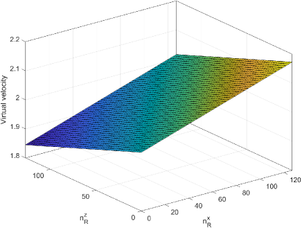
Fig. 4 shows an example of virtual velocity estimation and fitting. It can be seen from the figure that different antennas have observed different virtual velocities for the same dynamic target, the 2D antenna index and virtual velocity form a plane in the 3D coordinate system, and thus we can recover the radial velocity, horizontal angular velocity, and pitch angular velocity of the target from these virtual velocities {(nRx,nRz,vˇk,l,nRx,nRzLong,vir)|nRx=0,1,,NRx1;nRz=0,1,,NRz1}\{(n_{R}^{x},n_{R}^{z},\check{v}^{Long,vir}_{k^{\prime},l,n^{x}_{R},n^{z}_{R}})|n_{R}^{x}=0,1,...,N^{x}_{R}-1;n_{R}^{z}=0,1,...,N^{z}_{R}-1\} based on formulas from (58) to (64).

III-F Long-Term Motion Tracking

We consider the 6D motion parameters of the kk-th dynamic target 𝐒k,lLong\mathbf{S}^{Long}_{k,l} as the state of one micro-system, and consider the 𝐒ˇk,lLong\check{\mathbf{S}}^{Long}_{k,l} obtained through the 6D sensing algorithm as the observation of this micro-system. Based on the formulas from (8) to (13), the state equation can be expressed as

𝐒k,l+1Long=𝚽𝐒k,lLong+𝐁𝐮k,lLong+𝐰k,lLong,\begin{split}\begin{aligned} \mathbf{S}^{Long}_{k,l+1}=\mathbf{\Phi}\mathbf{S}^{Long}_{k,l}+\mathbf{B}\mathbf{u}^{Long}_{k,l}+\mathbf{w}_{k,l}^{Long},\end{aligned}\end{split} (65)

where 𝚽=[𝐈3×3TTTS𝐈3×3𝟎3×3𝐈3×3]\mathbf{\Phi}=\begin{bmatrix}\mathbf{I}_{3\times 3}&-T_{TTS}\mathbf{I}_{3\times 3}\\ \mathbf{0}_{3\times 3}&\mathbf{I}_{3\times 3}\end{bmatrix} is state transition matrix, 𝐁=[12TTTS2𝐈3×3TTTS𝐈3×3]\mathbf{B}=\begin{bmatrix}-\frac{1}{2}T_{TTS}^{2}\mathbf{I}_{3\times 3}\\ -T_{TTS}\mathbf{I}_{3\times 3}\end{bmatrix} is disturbance driven matrix, 𝐰k,lLong\mathbf{w}_{k,l}^{Long} is the state noise matrix and its covariance matrix is 𝐐\mathbf{Q}. Besides, the observation equation of the micro-system can be represented as

𝐒ˇk,lLong=𝐆𝐒k,lLong+𝐯k,lLong,\begin{split}\begin{aligned} \check{\mathbf{S}}^{Long}_{k,l}=\mathbf{G}\mathbf{S}^{Long}_{k,l}+\mathbf{v}_{k,l}^{Long},\end{aligned}\end{split} (66)

where 𝐆=𝐈6×6\mathbf{G}=\mathbf{I}_{6\times 6} is the observation matrix, 𝐯k,lLong\mathbf{v}_{k,l}^{Long} is equivalent observation noise vector and its covariance matrix is 𝐑\mathbf{R}. Then we can use Kalman filtering (KF) [34] to track the long-term motion of the kk-th dynamic target as follows:

1) Initialization: ISAC BS can obtain the 6D parameters estimation 𝐒kSBS\mathbf{S}^{SBS}_{k} of the kk-th dynamic target through beam scanning during SBS stage. Next, to enter the SBT stage, we initialize the time as l=0l=0, the observation as 𝐒ˇk,0Long=𝐒kSBS\check{\mathbf{S}}^{Long}_{k,0}=\mathbf{S}^{SBS}_{k}, the state estimation as 𝐒^k,0Long=𝐒kSBS\hat{\mathbf{S}}^{Long}_{k,0}=\mathbf{S}^{SBS}_{k}, and 𝐏^k,0=𝐈6×6\hat{\mathbf{P}}_{k,0}=\mathbf{I}_{6\times 6}.

2) State prediction: Based on 𝐒^k,l1Long\hat{\mathbf{S}}^{Long}_{k,l-1}, the state prediction within the ll-th TTS can be calculated as 𝐒~k,lLong=𝚽𝐒^k,l1Long\tilde{\mathbf{S}}^{Long}_{k,l}=\mathbf{\Phi}\hat{\mathbf{S}}^{Long}_{k,l-1}.

3) Observation prediction: The observation prediction within the ll-th TTS can be computed as 𝐒ˇ~k,lLong=𝐆𝐒~k,lLong\tilde{\check{\mathbf{S}}}^{Long}_{k,l}=\mathbf{G}\tilde{\mathbf{S}}^{Long}_{k,l}.

4) Calculate Kalman gain: Based on 𝐏^k,l1\hat{\mathbf{P}}_{k,l-1}, we can compute 𝐏~k,l=𝚽𝐏^k,l1𝚽T\tilde{{\mathbf{P}}}_{k,l}=\mathbf{\Phi}\hat{\mathbf{P}}_{k,l-1}\mathbf{\Phi}^{T}. Then the Kalman gain can be obtained as 𝐊k,lgain=𝐏~k,l𝐆T(𝐆𝐏~k,l𝐆T+𝐑)1\mathbf{K}^{gain}_{k,l}=\tilde{{\mathbf{P}}}_{k,l}\mathbf{G}^{T}\left(\mathbf{G}\tilde{{\mathbf{P}}}_{k,l}\mathbf{G}^{T}+\mathbf{R}\right)^{-1}.

5) State estimation update: The KF estimation of the 6D motion parameters can be updated and represented as 𝐒^k,lLong=𝐒~k,lLong+𝐊k,lgain(𝐒ˇk,lLong𝐒ˇ~k,lLong)\hat{\mathbf{S}}^{Long}_{k,l}=\tilde{\mathbf{S}}^{Long}_{k,l}+\mathbf{K}^{gain}_{k,l}({\check{\mathbf{S}}}^{Long}_{k,l}-\tilde{\check{\mathbf{S}}}^{Long}_{k,l}). Besides, 𝐏^k,l\hat{\mathbf{P}}_{k,l} can be updated as 𝐏^k,l=(𝐈6×6𝐊k,lgain𝐆)𝐏~k,l\hat{\mathbf{P}}_{k,l}=(\mathbf{I}_{6\times 6}-\mathbf{K}^{gain}_{k,l}\mathbf{G})\tilde{{\mathbf{P}}}_{k,l}.

Based on the above steps, we can continuously track the dynamic targets within LL TTS, and we employ 𝐒^k,lLong\hat{\mathbf{S}}^{Long}_{k,l} as the final 6D motion parameters estimation result of the kk-th dynamic target within the ll-th TTS.

Refer to caption
(a)
Refer to caption
(b)
Refer to caption
(c)
Refer to caption
(d)
Figure 5: (a) The RMSEϕ{\rm RMSE}_{\phi} versus SNR curves of different targets. (b) The RMSEr{\rm RMSE}_{r} versus SNR curves of different targets. (c) The RMSEvr{\rm RMSE}_{v_{r}} versus SNR curves of different targets. (d) The RMSEωϕ{\rm RMSE}_{\omega_{\phi}} versus SNR curves of different targets.

IV Simulation Results

In simulations, we set the lowest carrier frequency of the ISAC system as f0=100f_{0}=100 GHz, set the subcarrier frequency interval as Δf=480\Delta f=480 kHz, and set the antenna spacing as d=12λd=\frac{1}{2}\lambda. To succinctly display the simulation results, we set the horizontal angle and horizontal angular velocity of the dynamic target as θk=90\theta_{k}=90^{\circ} and ωθ,k=0\omega_{\theta,k}=0, and thus the dynamic target is fixed to move within a 2D plane. Then we focus on the sensing accuracy of the {rk,ϕk,vr,k,ωϕ,k}\{r_{k},\phi_{k},v_{r,k},\omega_{\phi,k}\} parameters of the dynamic target.

Specifically, for the aspect of evaluating 6D radar sensing, the root mean square error (RMSE) of distance sensing, angle sensing, radial velocity sensing and angular velocity sensing are defined as RMSEr=i=1Count(rˇs(i)rs)2Count{\rm RMSE}_{r}=\sqrt{\frac{\sum_{i=1}^{Count}(\check{r}_{s(i)}-r_{s})^{2}}{Count}}, RMSEϕ=i=1Count(ϕˇs(i)ϕs)2Count{\rm RMSE}_{\phi}=\sqrt{\frac{\sum_{i=1}^{Count}(\check{\phi}_{s(i)}-\phi_{s})^{2}}{Count}}, RMSEvr=i=1Count(vˇr,s(i)vr,s)2Count{\rm RMSE}_{v_{r}}=\sqrt{\frac{\sum_{i=1}^{Count}(\check{v}_{r,s(i)}-v_{r,s})^{2}}{Count}}, and RMSEωϕ=i=1Count(ωˇϕ,s(i)ωϕ,s)2Count{\rm RMSE}_{\omega_{\phi}}=\sqrt{\frac{\sum_{i=1}^{Count}(\check{\omega}_{\phi,s(i)}-\omega_{\phi,s})^{2}}{Count}}, where CountCount is the number of the Monte Carlo runs, the real parameters of the dynamic target is (rs,ϕs,vr,s,ωϕ,s)(r_{s},\phi_{s},v_{r,s},\omega_{\phi,s}), and (rˇs,ϕˇs,vˇr,s,ωˇϕ,s)(\check{r}_{s},\check{\phi}_{s},\check{v}_{r,s},\check{\omega}_{\phi,s}) is the estimation parameters of the target.

Refer to caption
(a)
Refer to caption
(b)
Refer to caption
(c)
Figure 6: (a) Distance sensing performance under different numbers of OFDM symbols. (b) Radial velocity sensing performance under different numbers of OFDM symbols. (c) Angular velocity sensing performance under different numbers of OFDM symbols.
Refer to caption
(a)
Refer to caption
(b)
Refer to caption
(c)
Figure 7: (a) Distance sensing performance under different numbers of subcarriers. (b) Radial velocity sensing performance under different numbers of subcarriers. (c) Angular velocity sensing performance under different numbers of subcarriers.

IV-A The Performance of 6D Radar Single-Shot Sensing

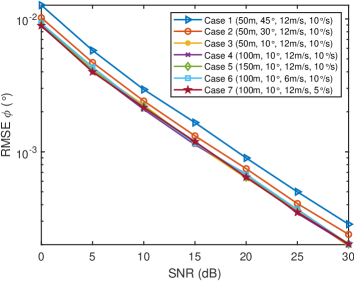
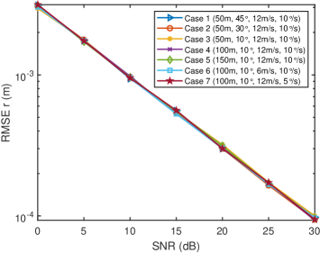
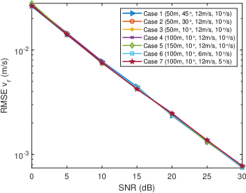
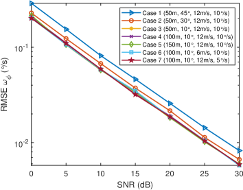
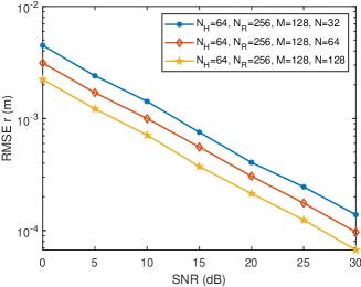
We set that the number of subcarriers is M=128M=128, the number of OFDM symbols is N=64N=64, the number of the antennas in HU-UPA is NH=64N_{H}=64, the number of the antennas in RU-UPA is NR=256N_{R}=256. Fig. 5 shows the single-shot sensing RMSE of the proposed scheme for different dynamic targets with different motion parameters versus SNR. It can be seen that the RMSEϕ{\rm RMSE}_{\phi}, RMSEr{\rm RMSE}_{r}, RMSEvr{\rm RMSE}_{v_{r}}, and RMSEωϕ{\rm RMSE}_{\omega_{\phi}} gradually decrease with the increase of SNR. When SNR =0=0 dB, the average sensing RMSEs are RMSEϕ=0.0097{\rm RMSE}_{\phi}=0.0097^{\circ}, RMSEr=0.0031m{\rm RMSE}_{r}=0.0031m, RMSEvr=0.0267m/s{\rm RMSE}_{v_{r}}=0.0267m/s, and RMSEωϕ=0.2208/s{\rm RMSE}_{\omega_{\phi}}=0.2208^{\circ}/s. When SNR increases to 2020 dB, the average sensing RMSEs decrease to RMSEϕ=0.0007{\rm RMSE}_{\phi}=0.0007^{\circ}, RMSEr=0.0003m{\rm RMSE}_{r}=0.0003m, RMSEvr=0.0024m/s{\rm RMSE}_{v_{r}}=0.0024m/s, and RMSEωϕ=0.0200/s{\rm RMSE}_{\omega_{\phi}}=0.0200^{\circ}/s.

Unlike most existing ISAC studies believing that only the radial velocity of far-field dynamic target can be measured based on one single BS. These simulation results indicate that the proposed 6D radar sensing algorithm has high sensing accuracy, especially confirming that one single BS with MIMO array can effectively estimate the angular velocity of the dynamic target.

Besides, it is found from Fig. 5(b) and Fig. 5(c) that under the same system parameter settings, the distance sensing and radial velocity sensing performance of dynamic targets with different motion parameters are basically consistent. However, it is seen from Fig. 5(a) and Fig. 5(d) that under the same system parameter settings, the accuracy of dynamic target angle sensing and angular velocity senisng gradually improves as the target approaches 00^{\circ}, mainly because the MIMO array has narrower beamwidth near 00^{\circ}, thus improving the accuracy of angle sensing. Since the angular velocity sensing depends on the angle change of the target, the narrower beam near 00^{\circ} also brings higher angular velocity sensing accuracy.

IV-B The Impact of System Parameters on the Performance of 6D Radar Single-Shot Sensing

We take the sensing of the dynamic target with motion parameters (ϕ=20\phi=20^{\circ}, r=120mr=120m, vr=15m/sv_{r}=15m/s, ωϕ=8/s\omega_{\phi}=8^{\circ}/s) as the example, and investigate the impact of system parameter settings on the performance of 6D radar single-shot sensing.

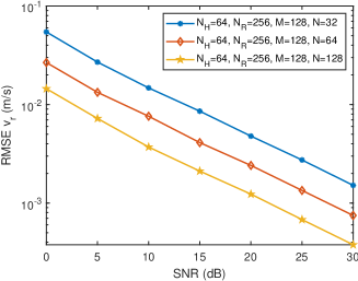
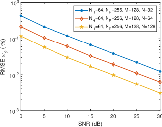
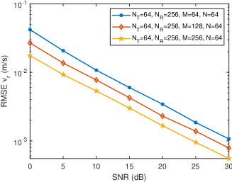
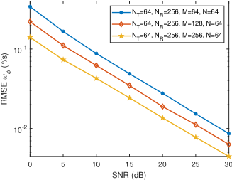
Fig. 6 shows the variation curves of distance sensing, radial velocity sensing, and angular velocity sensing versus SNR under different number of OFDM symbols. It can be seen from Fig. 6(a) that the RMSEr{\rm RMSE}_{r} gradually decreases as the number of OFDM symbols NN increases. This is because more OFDM symbols bring more observations to the distance array, making the estimation of the covariance matrix of the distance array more accurate, and thereby improving the accuracy of distance sensing. Besides, it can be found from Fig. 6(b) and Fig. 6(c) that the RMSEvr{\rm RMSE}_{v_{r}} and the RMSEωϕ{\rm RMSE}_{\omega_{\phi}} significantly decrease with the increase of NN. This is because more OFDM symbols form a larger virtual velocity array, making the sensing of radial velocity and angular velocity more accurate.

Refer to caption
(a)
Refer to caption
(b)
Refer to caption
(c)
Figure 8: (a) Distance sensing performance under different numbers of receiving antennas. (b) Radial velocity sensing performance under different numbers of receiving antennas. (c) Angular velocity sensing performance under different numbers of receiving antennas.
Refer to caption
Figure 9: The performance of multiple-shots tracking.

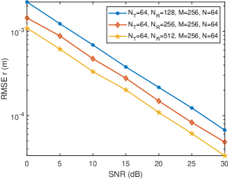
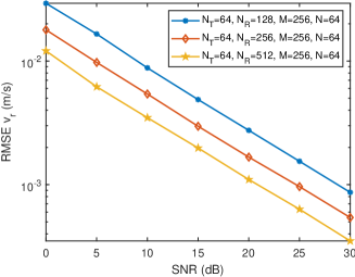
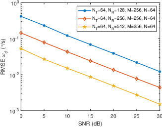
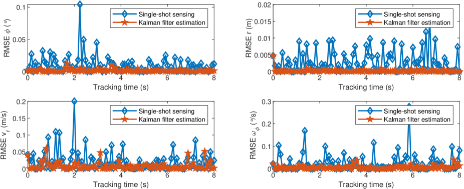
Fig. 7 shows the variation curves of sensing RMSEs versus SNR under different number of subcarriers. It can be seen from Fig. 7(a) that the RMSEr{\rm RMSE}_{r} gradually decreases with the increase of the number of subcarriers MM, because more subcarriers can form a larger distance array, thereby improving the accuracy of distance sensing. It can be found from Fig. 7(b) and Fig. 7(c) that the RMSEvr{\rm RMSE}_{v_{r}} and the RMSEωϕ{\rm RMSE}_{\omega_{\phi}} gradually decrease with the increase of MM. This is because more subcarriers bring more observations to the virtual velocity array, making the covariance matrix estimation of the virtual velocity array more accurate, thereby improving the sensing accuracy of radial velocity and angular velocity.

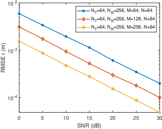
Fig. 8 shows the variation curves of sensing RMSEs versus SNR under different number of antennas. It can be seen from Fig. 8(a) that RMSEr{\rm RMSE}_{r} gradually decreases as the number of antennas NRN_{R} increases. This is because more receiving antennas provide more observations for distance array, thereby improving the accuracy of distance sensing. More importantly, it can be observed from Fig. 8(b) and Fig. 8(c) that the RMSEvr{\rm RMSE}_{v_{r}} and the RMSEωϕ{\rm RMSE}_{\omega_{\phi}} gradually decrease with the increase of NRN_{R}. This is because when there are more receiving antennas measuring the virtual velocity, the system can better fit the virtual velocity plane, thereby more accurately recovering the radial velocity and angular velocity of dynamic target.

IV-C The Performance of Multiple-Shots Tracking

We set the dynamic target with the initial motion parameter of ϕ=55\phi=55^{\circ}, r=100mr=100m, vr=8m/sv_{r}=8m/s, ωϕ=4/s\omega_{\phi}=4^{\circ}/s, and the BS needs to track this target within 88 seconds. We set the system parameters as M=128M=128, N=64N=64, NH=64N_{H}=64, and NR=256N_{R}=256. Fig. 9 shows the tracking performance of multiple-shots tracking for dynamic target when SNR =0=0 dB. It can be seen from the figure that the dynamic target tracking algorithm based on Kalman filtering can further improve the sensing accuracy of 6D radar single-shot sensing, especially the performance of angular velocity sensing. These simulation results verify the effectiveness of the proposed scheme.

V Conclusions

In this paper, we have proposed a novel scheme for 6D radar sensing and tracking of dynamic target based on MIMO array for monostatic ISAC system. We have re-examined and re-derived the relationship between 6D motion parameters of dynamic target and sensing echo channel of MIMO-ISAC system, and found that the sensing echo channel actually includes the distance, horizontal angle, pitch angle, radial velocity, horizontal angular velocity, and pitch angular velocity of dynamic target. Specifically, we have proposed the 6D long-term motion and short-term motion model of dynamic target. Then we have derived the sensing channel model corresponding to short-term motion. Next, for single-shot sensing, we employed the array signal processing methods to estimate the dynamic target’s distance, horizontal angle, pitch angle, and virtual velocity. Then we found that the virtual velocities observed by different antennas were different, which allowed us to utilize plane parameter fitting to estimate the radial velocity, horizontal angular velocity, and pitch angular velocity of the dynamic target. Furthermore, we have realized the multiple-shots tracking of dynamic target based on each single-shot sensing results and Kalman filtering. Simulation results have been provided to demonstrate the effectiveness of the proposed 6D radar sensing and tracking scheme.

References

  • [1] A. Hassanien, M. G. Amin, E. Aboutanios, and B. Himed, “Dual-function radar communication systems: A solution to the spectrum congestion problem,” IEEE Signal Process. Mag., vol. 36, no. 5, pp. 115–126, Sep. 2019.
  • [2] F. Liu, C. Masouros, A. P. Petropulu, H. Griffiths, and L. Hanzo, “Joint radar and communication design: Applications, state-of-the-art, and the road ahead,” IEEE Trans. Commun., vol. 68, no. 6, pp. 3834–3862, Feb. 2020.
  • [3] F. Liu, Y. Cui, C. Masouros, J. Xu, T. X. Han, Y. C. Eldar, and S. Buzzi, “Integrated sensing and communications: Toward dual-functional wireless networks for 6G and beyond,” IEEE J. Sel. Areas Commun., vol. 40, no. 6, pp. 1728–1767, Jun. 2022.
  • [4] M. Giordani, M. Polese, M. Mezzavilla, S. Rangan, and M. Zorzi, “Toward 6G networks: Use cases and technologies,” IEEE Commun. Mag., vol. 58, no. 3, pp. 55–61, Mar. 2020.
  • [5] Y. Cui, F. Liu, X. Jing, and J. Mu, “Integrating sensing and communications for ubiquitous IoT: Applications, trends, and challenges,” IEEE Network, vol. 35, no. 5, pp. 158–167, Nov. 2021.
  • [6] C. Chaccour, M. N. Soorki, W. Saad, M. Bennis, P. Popovski, and M. Debbah, “Seven defining features of terahertz (THz) wireless systems: A fellowship of communication and sensing,” IEEE Commun. Surveys Tuts., vol. 24, no. 2, pp. 967–993, Jan. 2022.
  • [7] Z. Wei, F. Liu, C. Masouros, N. Su, and A. P. Petropulu, “Toward multi-functional 6G wireless networks: Integrating sensing, communication, and security,” IEEE Commun. Mag., vol. 60, no. 4, pp. 65–71, Apr. 2022.
  • [8] S. Lu, F. Liu, and L. Hanzo, “The degrees-of-freedom in monostatic ISAC channels: NLoS exploitation vs. reduction,” IEEE Trans. Veh. Technol., vol. 72, no. 2, pp. 2643–2648, Feb. 2023.
  • [9] Z. Han, L. Han, X. Zhang, Y. Wang, L. Ma, M. Lou, J. Jin, and G. Liu, “Multistatic Integrated Sensing and Communication System in Cellular Networks,” arXiv e-prints, p. arXiv:2305.12994, May 2023.
  • [10] X. Chen, Z. Feng, Z. Wei, X. Yuan, P. Zhang, J. Andrew Zhang, and H. Yang, “Multiple signal classification based joint communication and sensing system,” IEEE Trans. Wireless Commun., pp. 1–1, 2023.
  • [11] W. Jiang, D. Ma, Z. Wei, Z. Feng, and P. Zhang, “ISAC-NET: Model-driven deep learning for integrated passive sensing and communication,” arXiv e-prints, p. arXiv:2307.15074, July 2023.
  • [12] F. Liu, W. Yuan, C. Masouros, and J. Yuan, “Radar-assisted predictive beamforming for vehicular links: Communication served by sensing,” IEEE Trans. Wireless Commun., vol. 19, no. 11, pp. 7704–7719, Nov. 2020.
  • [13] Z. Du, F. Liu, W. Yuan, C. Masouros, Z. Zhang, S. Xia, and G. Caire, “Integrated sensing and communications for v2i networks: Dynamic predictive beamforming for extended vehicle targets,” IEEE Trans. Wireless Commun., vol. 22, no. 6, pp. 3612–3627, Jun. 2023.
  • [14] S. Sun and Y. D. Zhang, “4D automotive radar sensing for autonomous vehicles: A sparsity-oriented approach,” IEEE J. Sel. Topics Signal Process., vol. 15, no. 4, pp. 879–891, Jun. 2021.
  • [15] M. Lei, D. Yang, and X. Weng, “Integrated sensor fusion based on 4D MIMO radar and camera: A solution for connected vehicle applications,” IEEE Veh. Technol. Mag., vol. 17, no. 4, pp. 38–46, Dec. 2022.
  • [16] J. A. Nanzer, “Millimeter-wave interferometric angular velocity detection,” IEEE Trans. Microw. Theory Techn., vol. 58, no. 12, pp. 4128–4136, Dec. 2010.
  • [17] J. A. Nanzer, K. Kammerman, and K. S. Zilevu, “A 29.5 GHz radar interferometer for measuring the angular velocity of moving objects,” in Proc. IEEE Int. Microwave Symp. Digest, pp. 1–3, Jun. 2013.
  • [18] J. A. Nanzer and K. S. Zilevu, “Time-frequency measurement of moving objects using a 29.5GHz dual interferometric-Doppler radar,” in Proc. IEEE Antennas and Propagation Soc. Int. Symp., pp. 830–831, Jul. 2013.
  • [19] J. A. Nanzer, “On the resolution of the interferometric measurement of the angular velocity of moving objects,” IEEE Trans. Antennas Propag., vol. 60, no. 11, pp. 5356–5363, Nov. 2012.
  • [20] X. Wang, P. Wang, and V. C. Chen, “Simultaneous measurement of radial and transversal velocities using a dual-frequency interferometric radar,” in Proc. IEEE RadarConf, pp. 1–6, Apr. 2019.
  • [21] X. Wang, P. Wang, and V. C. Chen, “Simultaneous measurement of radial and transversal velocities using interferometric radar,” IEEE Trans. Aerosp. Electron. Syst., vol. 56, no. 4, pp. 3080–3098, Aug. 2020.
  • [22] P. Wang, H. Liang, X. Wang, and E. Aboutanios, “Transversal velocity measurement of multiple targets based on spatial interferometric averaging,” in Proc. IEEE Int. Radar Conf. (RADAR), pp. 709–713, Apr. 2020.
  • [23] Z. Gao, Z. Wan, D. Zheng, S. Tan, C. Masouros, D. W. K. Ng, and S. Chen, “Integrated sensing and communication with mmWave massive MIMO: A compressed sampling perspective,” IEEE Trans. Wireless Commun., vol. 22, no. 3, pp. 1745–1762, Mar. 2023.
  • [24] H. Chen, H. Sarieddeen, T. Ballal, H. Wymeersch, M.-S. Alouini, and T. Y. Al-Naffouri, “A tutorial on terahertz-band localization for 6G communication systems,” IEEE Commun. Surveys Tuts., vol. 24, no. 3, pp. 1780–1815, May 2022.
  • [25] H. Luo, F. Gao, W. Yuan, and S. Zhang, “Beam squint assisted user localization in near-field integrated sensing and communications systems,” IEEE Trans. Wireless Commun., pp. 1–1, Oct. 2023.
  • [26] Z. Lin, T. Lv, J. A. Zhang, and R. P. Liu, “3D wideband mmwave localization for 5G massive MIMO systems,” in Proc. IEEE Global Commun. Conf. (GLOBECOM), Waikoloa, HI, USA, Dec. 2019, pp. 1–6.
  • [27] H. Luo, Y. Wang, J. Zhao, H. Wu, S. Ma, and F. Gao, “Integrated sensing and communications in clutter environment,” arXiv e-prints, p. arXiv:2311.01674, Nov. 2023.
  • [28] H. Luo, F. Gao, H. Lin, S. Ma, and H. V. Poor, “YOLO: An efficient terahertz band integrated sensing and communications scheme with beam squint,” arXiv e-prints, p. arXiv:2305.12064, May 2023.
  • [29] R. Roy and T. Kailath, “ESPRIT-estimation of signal parameters via rotational invariance techniques,” IEEE Trans. Acoust., Speech, Signal Process., vol. 37, no. 7, pp. 984–995, Jul. 1989.
  • [30] R. Roy, A. Paulraj, and T. Kailath, “ESPRIT–a subspace rotation approach to estimation of parameters of cisoids in noise,” IEEE Trans. Acoust., Speech, Signal Process., vol. 34, no. 5, pp. 1340–1342, Oct. 1986.
  • [31] A. Paulraj, R. Roy, and T. Kailath, “Estimation of signal parameters via rotational invariance techniques- esprit,” in Nineteeth Asilomar Conference on Circuits, Systems and Computers, 1985., pp. 83–89, Nov. 1985.
  • [32] M. Wax and T. Kailath, “Detection of signals by information theoretic criteria,” IEEE Trans. Acoust., Speech, Signal Process., vol. 33, no. 2, pp. 387–392, Apr. 1985.
  • [33] A. Barron, J. Rissanen, and B. Yu, “The minimum description length principle in coding and modeling,” IEEE Trans. Inf. Theory, vol. 44, no. 6, pp. 2743–2760, Oct. 1998.
  • [34] H. Ma, L. Yan, Y. Xia, and M. Fu, Introduction to Kalman Filtering, pp. 3–9. Singapore: Springer Singapore, 2020.