††thanks: marco.patriarca@kbfi.ee
A Bayesian Approach to the Naming Game Model
Abstract
Abstract.
We present a novel Bayesian approach to semiotic dynamics, which is a cognitive analogue of the naming game model restricted to two conventions.
The one-shot learning that characterizes the agent dynamics in the basic naming game is replaced by a word-learning process, in which agents learn a new word by generalizing from the evidence garnered through pairwise-interactions with other agents.
The principle underlying the model is that agents — like humans — can learn from a few positive examples and that such a process is modeled in a Bayesian probabilistic framework.
We show that the model presents some analogies but also crucial differences with respect to the dynamics of the basic two-convention naming game model.
The model introduced aims at providing a starting point for the construction of a general framework for studying the combined effects of cognitive and social dynamics.
Keywords:
Complex Systems, Language Dynamics, Bayesian Statistics, Cognitive Models, Consensus Dynamics, Semiotic Dynamics, naming game, Individual-Based Models
I Introduction
A basic question in complexity theory is how the interactions between the units of the system lead to the emergence of ordered states from initially disordered configurations Castellano-2009a ; Baronchelli-2018a . This general question concerns phenomena ranging from phase transitions in condensed matter systems and self-organization in living matter to the appearance of norm conventions and cultural paradigms in social systems. Various models were used in order to study social interactions and cooperation, e.g. models of condensed matter systems (such as spin systems), statistical mechanical models (e.g. based on the master equation), ecological competition models Castellano-2009a , many-agents game-theoretical models Xia-2017a ; Xia-2018a ; Zhang-2017a . Opinion dynamics and cultural spreading models represent suitable theoretical frameworks for a quantitative description of the emergence of social consensus Baronchelli-2018a .
In this respect, the emergence of human language remains a challenging, multi-fold question, related in turn to biological, ecological, social, logical, and cognitive aspects Mufwene-2001a ; Lass1997 ; Berruto-2004a ; Edelman-2007a ; Tenenbaum-1999 . Language dynamics Wichmann-2008b ; Wichmann-2008c has provided models describing phenomena of language competition and change that focus on the mutual interactions of linguistic traits (sounds, phonemes, grammatical rules, or languages understood as fixed entities) under the influence of ecological and social factors, modeling such interactions in analogy to biological competition and evolution.
However, the basic learning process of a word has a complex dynamics due to its cognitive dimension. In fact, learning a word means to learn a concept (understood as a pointer to a subset of objects, see Refs. Tenenbaum-1999 ; Tenenbaum-2000a ; Xu-2007a ) and a linguistic label —for example the name of the object— used for communicating the concept. The double conceptname nature of words has been studied through semiotic dynamics models, such as the models of Hurford Hurford-1989a and Nowak Nowak-1999a (see also Nowak-2000a ; Trapa-2000a ) and the naming game (NG) model Baronchelli-2006c ; guanrong2019 .
In the basic version of the model of Nowak Nowak-1999a , the language spoken by each agent () is defined by two personal matrices, representing the links of a bipartite network joining names and concepts: (1) an active matrix representing the conceptname links, where the element () gives the probability that agent will utter the th name to communicate the th concept; (2) the passive matrix , representing the nameconcept links, in which the element represents the probability that an agent interprets the th name as referring to the th concept. In the models of Hurford and in the model of Nowak, the languages of each individual evolve with time according to a game-theoretical dynamics, with agents gaining a reproductive advantage if their matrices have a higher communication efficiency. These studies have achieved interesting results, such as the emergence of non-ambiguous one-to-one links between objects and sounds, and explain why homonyms are more frequent than synonyms Hurford-1989a ; Nowak-1999a ; Nowak-2000a ; Trapa-2000a .
In the NG model Baronchelli-2006c ; guanrong2019 there is only one concept () that can be linked to a set of different names. The model can be reformulated through the agents’ lists of the nameconcept connections known to each agent . In the case of two-conventions models, where the conventions are the names and , the list of the th agent can be (no connection), or (one name is known), or (both nameconcept connections are known).
Extending semiotic dynamics models is not trivial and already two-opinion variants of the NG model, taking into account committed groups, show a remarkable phase diagram Xie-2012a ; and trying to describe actual cognitive effects requires entirely new features Fan-2018a . This paper presents a minimal model to study the interplay of the cognitive and social dynamical dimensions, assuming for simplicity the two-conventions NG model as a semiotic framework Baronchelli-2016a ; guanrong2019 and making a cognitive generalization within the experimentally validated Bayesian framework of Tenenbaum-1999 (see also Refs. Tenenbaum2001 ; Tenenbaum-2000a ; Griffiths2006 ; Xu-2007a ; Perfors-2011a ; Lake2015 ). In that framework, an individual can learn a concept from a small number of examples, a most remarkable feature of human learning Tenenbaum-1999 ; Tenenbaum-1999b ; Tenenbaum-2011a , to be contrasted with machine learning algorithms, which require a large amount of examples for generalizing successfully barber2012 ; Murphy-2012a ; Evgeniou-2000a .
The paper is organized as follows. The new model is introduced in Sec. II. In Sec. III, we present and discuss the features of the semiotic dynamics emerging from the numerical simulations and quantitatively compare them with those of the two-conventions NG model. Future directions in the study of the interplay of the cognitive and the social dynamics are outlined in Sec. V.
II A Bayesian learning approach to the naming game
II.1 The two-conventions naming game model
Before introducing the new model, we recall the basic 2-conventions NG model Castello2009 , in which there is a single concept , corresponding to an external object, and two possible names (synonyms) and for referring to . Thus, the possibility of homonymy is excluded Baronchelli-2016a . Each agent is equipped with the list of the names known to the agent. We assume that at each agent knows either or and has therefore a list or , respectively.
During a pair-wise interaction, an agent can act as a speaker, when conveying a word to another agent, or as a hearer, when receiving a word from a speaker. One can think of an agent conveying a word as uttering a name, e.g. , while pointing at an external object, corresponding to concept : thus, the hearer records not only the name but also the nameconcept association between and . At a later time , the list of the th agent can contain one or both names, i.e., , , or .
The system evolves according to the following update rules Baronchelli-2016a :
-
1.
Two agents and , the speaker and the hearer, respectively, are randomly selected.
-
2.
The speaker randomly extracts a name (here either or ) from the list and conveys it to the hearer . Depending on the state of agent , the communication is usually described as:
-
(a)
Success: the conveyed name is present also in the hearer’s list , i.e. also agent knows its meaning; then the two agents erase the other name from their lists, if present.
-
(b)
Failure: the conveyed name is not present in the hearer’s list ; then agent records and adds it to the list .
-
(a)
-
3.
Time is increased of one step, , and the simulation is reiterated from the first point above.
An example of unsuccessful and one of successful communication are schematized in the left panel (A) of Fig. 1, see Ref. Baronchelli-2006c for more examples. Despite its simple structure, the basic NG model describes the emergence of consensus about which name to use, which is reached for any (disordered) initial configuration baronchelli2007 .
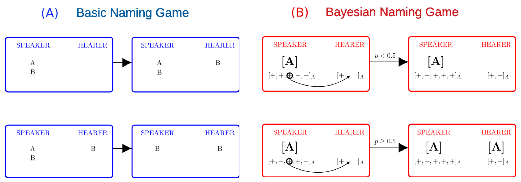
Panel (A): basic 2-conventions NG model. In a communication failure (upper figure), the name conveyed, in the example, is not present in the list of the hearer, who adds it to the list. In a communication success (lower figure), the word is already present in the hearer’s list and both agents erase from their lists.
Panel (B): Bayesian NG model; in order to convey an example “+” to the hearer in association with name , the speaker must have already generalized concept in association with , represented here by the label . In a communication failure (upper figure), the hearer computes the Bayes probability and the result is a ; then the only outcome is that the hearer records the example (reinforcement). In the Bayesian NG, there are two ways, in which the communication can be successful. The first way (lower figure) is when : the hearer generalizes in association with and attaches the label to the inventory. The second way (not shown) is the the agreement process, analogous to that of the basic NG, when both agents had already generalized concept in association with name and remove label from the inventory if present. See text for further details.
II.2 Toward a Bayesian naming game model
From a cognitive perspective, a “communication failure” of the NG model can be understood as a learning process, in which the hearer learns a new word. It is a “one-shot learning process”, because it takes place instantaneously (in a single time step) and independently of the the agent’s history (i.e. of the previous knowledge of the agent). However, modeling an actual learning process should take into account the agents’ experience, based on the previous observations (the data already acquired) as well as the uncertain/incomplete character naturally accompanying any learning process.
Here, the one-shot learning is replaced by a process that can describe basic but realistic situations, such as the prototypical “linguistic games” Wittgenstein1953 . For example, consider a “lecture game”, in which a lecturer (speaker) utters the name of an object and shows a real example “+” of the object to a student (hearer), repeating this process a few times. Then, the teacher can e.g. (a) show another example and ask the student to name the object; (b) utter the same name and ask the student to show an example of that object; or (c) do both things (uttering the name and showing the object) and ask the student whether the nameobject correspondence is correct. The student will not be able to answer correctly if not after having received some examples, enabling the student to generalize the concept corresponding to the object in association to name . To model these and similar learning processes, we need a criterion enabling the hearer to assess the degree of equivalence between the new example and a the examples recorded previously.
The starting point for the replacement of the one-shot learning is Bayes’ theorem. According to Bayes’ theorem, the posterior probability that the generic hypothesis is the true hypothesis, after observing a new evidence , reads Harney-2003a ; Jeffreys1961 ,
| (1) |
Here, the prior probability gives the probability of occurrence of the hypothesis before observing the data and gives the probability of observing if is given. Finally, gives the normalization constraint; in the applications it can be evaluated as , where represents the set of hypotheses, within the hypothesis space .
The next step is to find a way to compute explicitly the posterior probability , through a representation of the concepts and their relative examples in a suitable hypothesis space of the possible extensions of a given concept , constituted by the mutually exclusive and exhaustive hypotheses . Following the experimentally verified Bayesian statistical framework of Refs. Tenenbaum-1999 ; Tenenbaum-1999b , we adopt the paradigmatic representation of a concept as a geometrical shape. For example, the concept of “healthy level” of an individual in terms of the levels of cholesterol and insulin , defined by the ranges and , where and () are suitable values, represents a rectangle in the Euclidean - plane . Examples of healthy levels of specific individuals correspond to points . In the following, we assume that a hypothesis is represented by a rectangular region in . Figure 2 shows four positive examples, denoted by the symbol “+”, associated to four different points of the plane, consistent with (i.e. contained in) three different hypotheses, shown as rectangles.
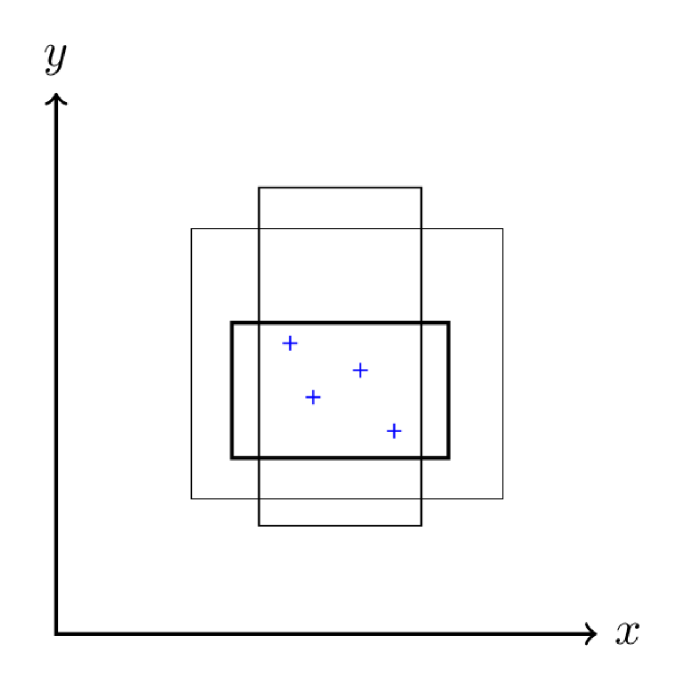
The problem of learning a word is now recast into an equivalent problem, consisting in acquiring the ability to infer whether a new example recorded, corresponding to a new point “+” in , corresponds to the concept , after having seen a small set of positive examples “+” of . More precisely, let be a sequence of examples of the true concept , already observed by the hearer, and the new example. The learner does not know the true concept , i.e. the exact shape of the rectangle associated to , but can compute the generalization function by integrating the predictions of all hypotheses , weighted by their posterior probabilities :
| (2) |
Clearly, if and otherwise. By means of the Bayes’ theorem (1), one can obtain the right Bayesian probability for the problem at hand. A successful generalization is then defined quantitatively by introducing a threshold , representing an acceptance probability: an agent will generalize if the Bayesian probability . The value is assumed, as in Ref. Tenenbaum-1999b .
We assume that an Erlang prior characterizes the agents’ background knowledge. For a rectangle in defined by the tuple , where are the Cartesian coordinates of its lower-left corner and its sides along dimension , the Erlang prior density is Tenenbaum-1999 ; Tenenbaum-1999b
| (3) |
where the parameters represent the actual sizes of the concept, i.e. they are the sides of the concept rectangle along dimension . The choice of a specific informative prior, such as the Erlang prior, is well motivated by the fact that in the real world individuals have always some prior knowledge or expectation. In fact, a Bayesian learning framework with an Erlang prior of the form (3) well describes experimental observations of learning processes of human beings Tenenbaum-1999b . The final expression used below for computing the Bayesian probability that, given the set of previous examples , the new example falls in the same category of concept , reads Tenenbaum-1999b
| (4) |
Here () is an estimate of the extension of the set of examples along direction , given by the maximum mutual distance along dimension between the examples of ; measures an effective distance between the new example and the previously recorded examples, i.e., if falls inside the value range of the examples of along dimension , otherwise is the distance between and the nearest example in along the dimension . Equation (4) is actually a “quick-and-dirty” approximation that is reasonably good, except for and , estimating the actual generalization function within a error, see Refs. Tenenbaum-1999 ; Tenenbaum-1999b for details. Despite these approximations, Eq. (4) will ensure that our computational model, described in the next section, retains the main features of the Bayesian learning framework. It is to be noticed that for the validity of the Bayesian framework, it is crucial that the examples are drawn randomly from the concept (strong sampling assumption), i.e. they are extracted from a probability density that is uniform in the rectangle corresponding to the true concept Tenenbaum-1999b . This definition of generalization is now applied below to word-learning.
II.3 The Bayesian word-learning model
Based on the Bayesian learning framework discussed above, in this section we introduce a minimal Bayesian individual-based model of word-learning. For the sake of clarity, in analogy with the basic NG model, we study the emergence of consensus in the simple situation, in which two names and can be used for referring to the same concept in pair-wise interactions among agents.
At variance with the NG model, here in each basic pair-wise interaction an agent , acting as a speaker, conveys an example “+” of concept , in association with either name or , to another agent , who acts as hearer (). In order to be able to communicate concept uttering a name, e.g. name , the speaker must have already generalized concept in association with name . This is signalled by the presence of name in the list . On the other hand, the hearer always records the example received in the respective inventory, in the example the inventory .
The state of a generic agent at time is defined by
-
•
the list , to which a name is added whenever agent generalizes concept in association with that name; agent can use any name in to communicate ;
-
•
two inventories and , containing the examples “+” of concept received from the other agents in association with name and , respectively.
It is assumed that initially each agent knows one word: a fraction of the agents know concept in association with name and the remaining fraction in association with name — no agent knows both words, . We will examine three different initial conditions:
| symmetric initial conditions | (SIC): | ||||
| asymmetric initial conditions | (AIC): | ||||
| reversed case of AIC | (AICr): |
Initially, each agent , within the fraction of agents that know name , is assigned examples “+” of concept in association with name , but no examples in association with the other name , so that agent has an -inventory and an empty -inventory . The complementary situation holds for the other agents that know only name , who initially receive examples of concept in association with name but none in association with . This choice, somehow arbitrary, is dictated by the condition that Eq. (4) becomes a good approximation for Tenenbaum-1999 .
Examples are points uniformly generated inside the fixed rectangle corresponding to the true concept , here assumed to be a rectangle with lower left corner coordinates and sizes and along the and axis, respectively. Results are independent of the assumed numerical values; in particular, no appreciable variation in the convergence times is observed as the rectangle area is varied, which is consistent with the strong sampling assumption, on which the Bayesian learning framework rests; see Ref. Tenenbaum-1999 and Sec. III.
Furthermore, we introduce an element of asymmetry between the names and , related to the word-learning process: different minimum numbers of examples and will be used, which are needed by agents to generalize concept in association with and , respectively. This is equivalent to assume that concept is slightly easier to learn in association with name than . Such an asymmetry plays a relevant role in the model dynamics in differentiating the Bayesian generalization functions and from each other, see Sec. IV.
The dynamics of the model can be summarized by the following update rules:
-
1.
A pair of agents and , acting as speaker and hearer, respectively, are randomly chosen among the agents.
-
2.
The speaker selects randomly: (a) a name from the list (or selects the name present if contains a single name), for example (analogous steps follow if the word is selected); (b) an example among those contained in the corresponding inventory — ;
then the speaker conveys the example extracted in association with (e.g. uttering) the name selected to the hearer . -
3.
The hearer adds the new example (in association with ) to the inventory . This reinforcement process of the hearer’s knowledge always takes place.
-
4.
Instead, the next step depends on the state of the hearer:
-
(a)
Generalization. If the selected name, in the example, is not present in the hearer’s list , then the hearer computes the relative Bayesian probability that the new example falls in the same category of concept , using the examples previously recorded in association with , i.e. from the set of examples . If , the hearer has managed to generalize concept and connects the inventory to name ; this is done by adding name to the list . Starting from this moment, agent can communicate concept to other agents by conveying an example taken from the inventory while uttering the name . If , the hearer has not managed to generalize the concept and nothing more happens (the reinforcement of the previous point is the only event taking place).
-
(b)
Agreement. The name uttered by the speaker, in the example, is present in the hearer’s list , meaning that that agent has already generalized concept in association with name and has connected the corresponding inventory to . In this case, the hearer and the speaker proceed to make an agreement — analogous to that of the NG model, leaving in their lists and and removing is present. No examples contained in any inventory are removed.
-
(a)
-
5.
Time is updated, , and the simulation is reiterated from the first point above.
Two examples of Bayesian word-learning process, a successful and an unsuccessful one, are illustrated in the cartoon in the right panel (B) of Fig. 1. Table 1 lists the possible encounter situations, together with the corresponding relevant probabilities.
Notice that an agent can enter a pair-wise interaction with a non-empty inventory of examples, e.g. , associated to name , without being able to use name to convey examples to other agents, i.e., without the name in the list due to not having generalized concept in association with . Those examples can have different origins: (1) in the initial conditions, when randomly extracted examples associated to and to are assigned to each agent; (2) in previous interactions, in which the examples were conveyed by other agents; (3) in an agreement about convention , which removed label from the list while leaving all the corresponding examples in the inventory associated to name . In the latter case, the inventory may be “ready” for a generalization process, since it contains a sufficient number of examples, i.e., agent will probably be able to generalize as soon as another example is conveyed by an agent. This situation is not as peculiar as it may look at first sight. In fact, there is a linguistic analogue in the case where a speaker that loses the habit to use a certain word (or a language) can regain it promptly, if exposed to again.
Notice also that without the agreement dynamics scheme introduced in the model, borrowed from the basic NG model, the population fraction of individuals who know both and () would be growing, until eventually .
| S-List | Name | H-List | Branching | Process | Condition | S- List | H-List |
| (before) | conveyed | (before) | probability | (after) | (after) | ||
| Reinforcement | always | ||||||
| Reinforcement | |||||||
| Learning | |||||||
| Agreement | always | ||||||
| Reinforcement | |||||||
| Learning | |||||||
| Reinforcement | always | ||||||
| Agreement | always | ||||||
| Agreement | always | ||||||
| Reinforcement | |||||||
| Learning | |||||||
| Reinforcement | |||||||
| Learning | |||||||
| Agreement | always | ||||||
| Agreement | always | ||||||
| Agreement | always |
III Results
In this section we study numerically the Bayesian NG model introduced above and discuss its main features. We limit ourselves to study the model dynamics on a fully-connected network.
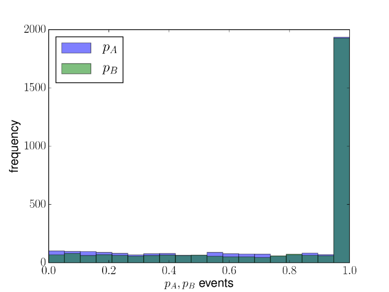
In the new learning scheme, which replaces the one-shot learning of the two-conventions NG model, an individual generalizes concept on a suitable time scale , rather than during a single interaction. However, a few examples are sufficient for an agent to generalize concept , as in a realistic concept-learning process. This is visible from the Bayesian probabilities and computed by agents in the role of hearer, according to Eq. (4), once at least and examples “+”, respectively, have been stored in the inventory associated to the name and : Figure 3 shows the histograms of the ’s and ’s computed from the initial time until consensus for a single run with agents and starting with SIC. The low frequencies at small values of and and the highest frequencies at values close to unity are due to the fact that the Bayesian probabilities reach values very fast, after a few learning attempts, consistently with the size principle, on which the Bayesian learning paradigm, and in turn Eq. (4), are based Tenenbaum-1999 .
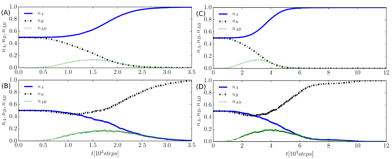
In order to visualize how the system approaches consensus, it is useful to consider some global observables, such as the fractions , , and of agents that have generalized concept in association with name only, name only, or both names and , respectively, or the success rate . The dynamics of a population of agents (panels (A) and (B)) using different initial conditions, SIC, AIC, and AICr, and that of a population of agents starting with SIC (panels (C) and (D)) are shown in Fig. 4.
Panel (A) of Fig. 4 shows only the population fractions corresponding to the name found at consensus, for the sake of clarity (the remaining population fractions eventually go to zero). For asymmetrical initial condition (AIC or AICr), it is the initial majority that determines the convention found at consensus (that is for AIC and for AICr). If the system starts from SIC, the convention , for which agents can generalize earlier (), is always found at consensus — in this case it is the asymmetry in the thresholds and , characterizing the Bayesian learning process, to determine consensus.
Panel (B) of Fig. 4 shows the success rate , representing the average over different runs of the instantaneous success rate of the th interaction at time , defined as follows: in case of agreement between the two agents or when a successful learning of the hearer takes places, following a Bayes probability ; or in case of unsuccessful generalization, when and only reinforcement takes place. The success rate varies between , due to the respective fractions of agents that initially know the two conventions and , to at consensus, following a typical S-shaped curve of learning processes Baronchelli2006 . In the case of SIC, the initial value is , while for AIC or AICr the initial value is .
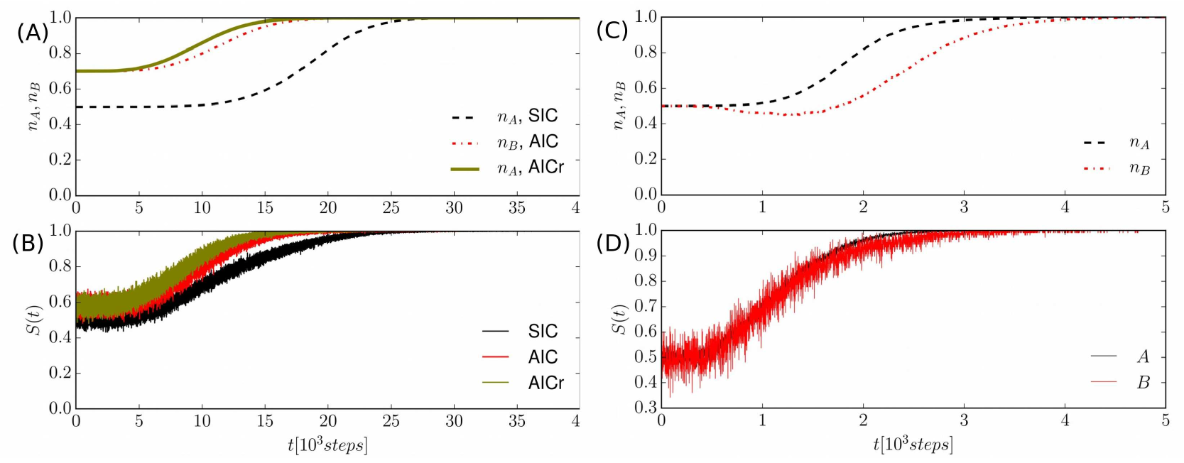
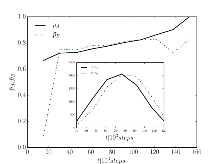
We now investigate how the modified Bayesian dynamics affects the convergence times to consensus. The study of the size-dependence of the convergence to consensus shows that there is a critical value in the case of SIC, such that for there is a non-negligible probability that the final absorbing state is . Panels (C) and (D) of Fig. 4, representing the results for a system starting with SIC and a smaller size , show the existence of two possible final absorbing states and that there are different times scales associated to the convergence to consensus: name is found at consensus in about of cases and name in the remaining cases. The branching probability into or consensus is further investigated in panel (A) of Fig. 5, where we plot the branching probabilities versus the system sizes . The nonlinear behavior (symmetrical sigmoid) signals the presence of finite-size effects, particularly clear for relatively small -values. In fact, when the fluctuations in the system are larger, the system size can play an important role in the dynamics of social systems, as an actual thermodynamic limit is only allowed for simulations of macroscopic physical systems Toral2007a .
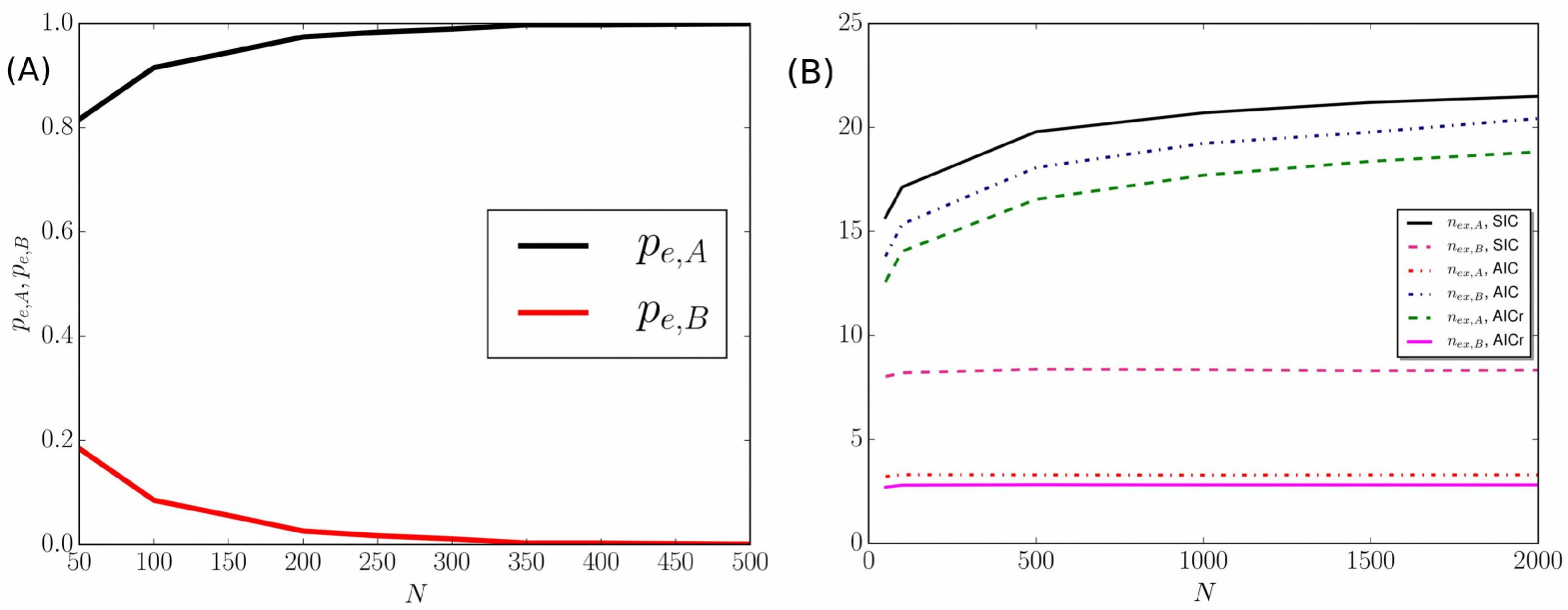
The convergence time follows a simple scaling rule with the system size , related to the average number of examples relative to respectively, stored in the agents’ inventories at consensus. These values depend on the number of learning and reinforcement processes, and hence are related to the system size . The average number of interactions undergone by the agents until the system reaches the consensus is given by the sum 111The examples given initially to each agent are not accounted for by and .. One expects that
| (5) |
which suggests a linear scaling law () for convergence time with the system size for all the possible initial conditions. A linear behavior is indeed confirmed by the numerical simulations with population sizes starting from SIC, AIC, AICr. The relative numerical results are reported in Table 2. Moreover, in Eq. (5) the size-dependence of is ignored as it shows a weak dependence upon , see panel (B) in Fig. 5.
| outcome | ||||
|---|---|---|---|---|
| SIC | ||||
| AIC | ||||
| AICr |
From the above mentioned scaling law, it is clear that the average number of examples stored by the agents at consensus plays an important role in the semiotic dynamics. In particular, it is found that if the final absorbing state is (or B), then ( ). Moreover, the average number of examples, relative to the absorbing state, always increases monotonically with the system size while a size-independent behavior is observed in the opposite case, see the right panel (B) of Fig. 5.
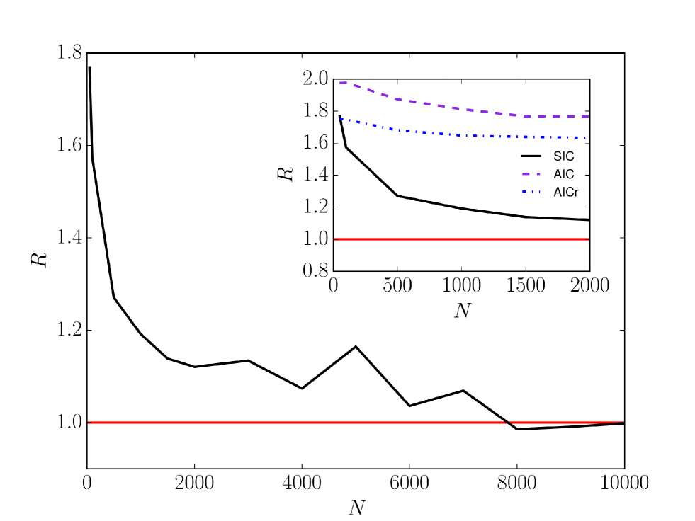
Finally, we compare the convergence time of the Bayesian word-learning model, , with that of two-conventions NG model, Castello2009 , by studying the corresponding ratio for common initial conditions and population sizes. When starting with SIC, the values of the convergence times obtained from the two models become of the same order by increasing : decreases with , reaching unity for , see Fig. 6. In other words, the time scales of the two models become equivalent for relatively large system sizes, i.e., the learning processes of the two models perform equivalently and the Bayesian approach roughly gives rise to the one-shot learning that characterizes the two-conventions NG model. In the next section we discuss how the Bayesian model becomes asymptotically equivalent to the minimal NG model. The inset of Fig. 6 represents versus , for , given different starting configurations, with SIC, AIC and AICr, and different population sizes. In the following, we focus on the case of SIC.
IV Stability analysis
In this section we investigate the stability properties of the mean-field dynamics of the Bayesian NG model, in which statistical fluctuations and correlations are neglected. In the Bayesian NG model, as in the basic NG, agents can use two non-excluding options and to refer to the same concept . The main difference between the Bayesian model and the basic NG model is in the learning process: a one-shot learning process in the basic NG and a Bayesian process in the Bayesian NG model. In the latter case the presence of a name in the word list indicates that the agent has generalized the corresponding concept from a set of positive recorded examples.
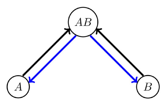
The NG model belongs to the wide class of models with two non-excluding options and , such as many models of bilingualism Patriarca2012a , in which transitions between state and state are allowed only through an intermediate (“bilingual”) state , as schematized in Fig. 7. The mean-field equations for the fractions and can be obtained considering the gain and loss contributions of the transitions depicted in Fig. 7,
| (6) |
Here and the quantities represent the respective transition rates per individual, corresponding to the arrows in Fig. 7 (). The equation for was omitted, since it is determined by the condition that the total number of agents is constant, .
The details of the possible pair-wise interactions in the Bayesian naming game are listed in Table 1. From the various contributions, one obtains the master equation
| (7) |
which can be rewritten in the form (IV) with transition rates per individual given by
| (8) | ||||||
| (9) |
Equations (8) provide the transition rates of learning processes, while Eqs. (9) give the transition rates of agreement processes. Setting , , and , the autonomous system (IV) becomes
| (10) | |||
| (11) |
where is the velocity field in the phase plane. For the following analysis, it is convenient to write the Bayesian probabilities and appearing in these equations as time-dependent parameters of the model, but they are actually highly non-linear functions of the variables. In fact, they can be thought as averages of the microscopic Bayesian probability in Eq. (4) over the possible dynamical realizations. For this reason, they have also a complex non-local time-dependence on the previous history of the interactions between agents. For the moment, we assume , returning later to the general case.
From the conditions defining the critical points, , one obtains . Setting , one obtains two solutions that correspond to consensus in or , given by and . Instead, setting leads to the equation
| (12) |
that has the solutions
| (13) |
For , the corresponding solutions are not suitable solutions, because .
This analysis is valid for . In fact, is a function of time and for a finite interval of time after the initial time one has that , which defines a different dynamical system. In the initial conditions used, , which implies , , and at any later time as long as , since (see Eq. (IV); in fact, the whole line (for ) represents a continuous set of equilibrium points. The reason why in this model at and also during a subsequent finite interval of time is twofold. First, agents do not have any examples associated to the name not known and they have to receive at least or examples, before being able to compute the corresponding Bayesian probability or — thus it is to be expected that meanwhile. Furthermore, even when agents can compute the Bayesian probabilities, the effective probability to generalize is actually zero, due to the threshold for a generalization to take place. The existence of the (temporary) equilibrium points on the line ends as soon as the parameter and, according to Eqs. (IV), the two - and -consensus states become the only stable equilibrium points. The representative point in the --plane is deemed to leave the initial conditions on the line, due to the stochastic nature of the dynamics, which is not invariant under time reversal hinrichsen2006 .
To determine the nature of the critical points and , one needs to evaluate at the equilibrium points the Jacobian matrix , where . It is easy to show that both the critical points and are asymptotically stable strogatz2000 .
As long as the general case , it can be shown that the trajectory of the system can point toward and eventually reach the consensus state with or , depending on whether or , where is the critical time at which the representative point leaves the initial position.
The convention or is selected randomly, depending on various factors related to the specific realization of the system evolution, such as the numbers of examples and recorded by the agents until time , their quality from the point of view of the generalization, and the initial asymmetry of the thresholds for generalizing, . The asymmetrical thresholds produce a bias toward consensus in and play a crucial role in the subsequent Bayesian semiotic dynamics; in fact, swapping the threshold values (setting ), the approach to consensus occurs with the outcomes , swapped.
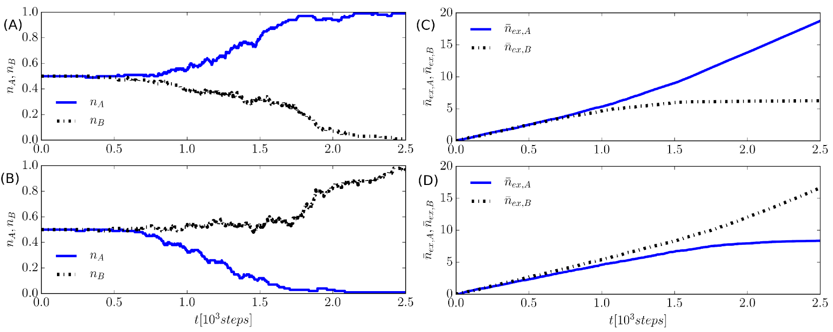
We observed that for , the chances that the system converges to become negligible. This can be seen in panels (C) and (D) of Fig. 8, showing and versus time (averaged over the agents of the system) for single runs, a population of agents, and SIC, for different runs that relax toward consensus and , respectively. After an initial transient, in which , they differ more and more from each other at times . In turn, also and begin to differ significantly from each other, thus affecting the rate of depletion of the populations during the subsequent dynamics. For instance, if , then , see Eqs. (8), which means that the depletion of occurs faster then that of . In turn, this favours the decay of the mixed states into the state , see Eqs. (9), being .
The asymmetry discussed above also affects the convergence times and and we find in all the numerical simulations. Despite the noise, such a trend is already appreciable in a single run, as shown in panels (A) and (B) of Fig. 8. The mean fractions , , and versus time, obtained by averaging over many runs, result in less noisy outputs and provide a more clear picture of the difference, which is visible in Fig. 9, obtained using runs starting with SIC and for agents (panels (A) and (B)) and agents (panels (C) and (D)). In addition, the convergence times depend on the system size, increasing with the number of agents : compare the left panels (A) and (B), where agents, with the right panels (C) and (D), where agents.
The possibility that the same system, starting with the same initial conditions and evolving with the same dynamical parameters, can reach either or is a consequence of the stochastic nature of dynamics. This does not happen for , when both and reach some threshold values close to those observed at , which is clearly a value sufficient for the agents to generalizing concept . In fact, the scaling law of with shows that the sum of with becomes nearly constant for , implying that the dynamics is uniquely determined, that is, the consensus always occurs at from SIC, once the agents have stored a threshold number of , . It is found that these threshold values correspond to , . Note that in , we add values the four initial given examples stored in the agents’ inventories at the beginning. The reason is that the generalization function outputs will effectively depend on them all. Therefore, at these threshold values, it would be very unlikely that , and so it would be the same for the consensus at .
Now we consider the Bayesian probabilities and computed by agents and the corresponding number of learning attempts and made by agents at time to learn concept in association with word or , respectively, i.e. the number of times that the agents compute or (only the case of a system starting with SIC is considered). We consider a single run of a system with agents and study the average values , obtained by averaging and over the agents of the system. We also assume a coarse-grained view, consisting in an additional average of , , and , , over a a temporal bin , in order to reduce random fluctuations. Figure 10 shows the time evolution of the average probabilities and in the time-range where data allow a good statistics. The probabilities grow monotonically and eventually reach the value one. While this points at an equivalence between the mean-field regime of the Bayesian naming game and that of the two-conventions NG model, in which agents learn at the first attempt (one-shoot learning), such an equivalence is suggested but not fully reproduced by the coarse-grained analysis. The time evolution of the number of learning attempts and shows that they are negligible both at the beginning and at the end of the dynamics — see inset in Fig. 10. This is due to the fact that at the beginning it is most likely that either interactions between agents with the same conventions take place (starting with SIC, each agent has a probability of 50% to interact with an agent having the same convention) or interactions between agents with different conventions but with still too small inventories to be able to generalize concept , leading to reinforcement processes only. When approaching consensus, agents with one of the conventions constitute the large majority of the population and thus they are again most likely to interact through reinforcements only. Thus, the largest numbers of attempt to learn concept in association with and are expected to occur at the intermediate stage of the dynamics. In fact, and are observed to reach a maximum at for any given system size , as visible in the inset of Fig. 10. Notice that also the fraction of agents , who know both conventions and can communicate using both name and name , possibly allowing other agents to generalize in association with name or , reaches its maximum roughly at the same time.
V Conclusion
We introduced a novel agent-based model that describes the appearance of linguistic consensus through a word-learning process. The work presented is exploratory in nature, concerning the minimal problem of a single concept that can be associated to two different possible names or , but is aimed at providing a prototype of general framework for describing the interaction between the social and the cognitive dimension. To this aim, the model is constructed on the basis of the semiotic dynamics of the NG model and is then extended by adding a Bayesian cognitive process, mimicking human learning processes.
The model describes in a natural way (1) the uncertainty accompanying the first phase of a learning process, (2) the gradual reduction of the uncertainty as more and more examples are provided, and (3) the ability to learn from a few examples. The semiotic dynamics of the synonyms is different from the basic NG, in that it depends on parameters that are of a strictly cognitive nature, such as the thresholds of the number of examples necessary before an agent can try to generalize and the acceptance threshold for carrying out the generalization of a concept. The interplay between the asymmetry of the conventions and , the system size, and the stochastic character of the time evolution, have dramatic consequences on the consensus dynamics: there is a critical time , when the system begins to move in the phase-plane to eventually converge toward a consensus state; there is a critical system size , such that for the system can end up in any of the two consensus states and the convergence times depends on ; there is an asymmetry in the branching probabilities that the system converges toward one of the two possible conventions and of the corresponding convergence times; the scaling laws of the convergence times versus differ from those observed in the basic NG model, because they depend on the learning experience of the agents.
The cognitive dimension offers additional possibilities for modelling in terms of specific cognitive parameters problems that are out of the reach of traditional social dynamics models. The model illustrated in this work represents a step toward a generalized Bayesian approach to social interactions, leading to cultural conventions.
Future work can address specific problems of current interest from the point of view of cognitive processes; or features relevant from the general standpoint of complexity theory. In the first case, it is possible to study in the cognitive dimension the semiotic dynamics of homonyms, synonyms, and innovation, e.g., the cognitive conditions leading to a name , associated to a concept , splitting into two names and , associated to two related but distinct concepts and , as more examples become available that make the two concepts eventually distinguishable from each other — a type of problems that cannot be tackled within models of cultural competition. In the second case, one can mention the classical problem of the interplay between a central information source (bias) and the local influences of individuals — this time in a cognitive framework.
Another question to be investigated within a cognitive framework would be the role of heterogeneity. In fact, heterogeneity is known to characterize most of the known complex systems at various levels — here the diversity could affect the dynamical parameters of e.g. the different competing names as well as those of the agents. Heterogeneity of individuals can lead to counter-intuitive effects, such as resonant behaviors Tessone2009a ; VazMartins2009a . Furthermore, the complex, heterogeneous nature of a local underlying social network can change drastically the co-evolution and the time-scales of the conventions in competition with each other Toivonen2009a .
Acknowledgements
The authors acknowledge support from the Estonian Ministry of Education and Research through Institutional Research Funding IUT (IUT39-1), the Estonian Research Council through Grant PUT (PUT1356), and the ERDF (European Development Research Fund) CoE (Center of Excellence) program through Grant TK133.
We also thank Andrea Baronchelli for providing useful remarks about the naming game model and the manuscript.
References
- (1) C. Castellano, S. Fortunato, and V. Loreto. Statistical physics of social dynamics. Rev. Mod. Phys., 81:591, 2009.
- (2) A. Baronchelli. The emergence of consensus: a primer. R. Soc. open sci., 5:172189, 2018.
- (3) C. Xia, S. Ding, C. Wang, J. Wang, and Z. Chen. Risk analysis and enhancement of cooperation yielded by the individual reputation in the spatial public goods game. IEEE Systems Journal, 11(3):1516–1525, Sep. 2017.
- (4) Chengyi Xia, Xiaopeng Li, Zhen Wang, and Matjaž Perc. Doubly effects of information sharing on interdependent network reciprocity. New Journal of Physics, 20(7):075005, jul 2018.
- (5) Yingchao Zhang, Juan Wang, Chenxi Ding, and Chengyi Xia. Impact of individual difference and investment heterogeneity on the collective cooperation in the spatial public goods game. Knowledge-Based Systems, 136:150 – 158, 2017.
- (6) S. Mufwene. The ecology of language evolution. Cambridge University Press, Cambridge, 2001.
- (7) R. Lass. Historical Linguistics and Language Change. Cambridge University Press, Cambridge, UK, 1997.
- (8) C. Berruto. Prima lezione di sociolinguistica. Laterza, Roma & Bari, 2004.
- (9) S. Edelman and H. Waterfall. Behavioral and computational aspects of language and its acquisition. Phys. Life Rev., 4:253–277, 2007.
- (10) J. B Tenenbaum. A Bayesian Framework For Concept Learning. PhD thesis, MIT, 1999.
- (11) S. Wichmann. The emerging field of language dynamics. Language and Linguistics Compass, 2/3:442, 2008.
- (12) S. Wichmann. Teaching & learning guide for: The emerging field of language dynamics. Language and Linguistics Compass, 2, 2008.
- (13) Joshua B. Tenenbaum and Fei Xu. Word learning as Bayesian inference. In Proceedings of the 22nd Annual Conference of the Cognitive Science Society, 2000.
- (14) F. Xu and J. B. Tenenbaum. Word learning as Bayesian inference. Psychological Review, 114:245–272, 2007.
- (15) J.R. Hurford. Biological evolution of the saussurean sign as a component of the language-acquisition device. Lingua, 77:187–222, 1989.
- (16) Martin A. Nowak, Joshua B. Plotkin, and David C. Krakauer. The evolutionary language game. Journal of Theoretical Biology, 200(2):147 – 162, 1999.
- (17) M.A. Nowak. Evolutionary biology of language. Philos. Trans. R. Soc. London B Biol. Sci., 355(1403):1615–22, 2000.
- (18) Peter E. Trapa and Martin A. Nowak. Nash equilibria for an evolutionary language game. Journal of Mathematical Biology, 41(2):172–188, Aug 2000.
- (19) Andrea Baronchelli, Maddalena Felici, Vittorio Loreto, Emanuele Caglioti, and Luc Steels. Sharp transition towards shared vocabularies in multi-agent systems. Journal of Statistical Mechanics: Theory and Experiment, 2006(06):P06014, 2006.
- (20) Guanrong Chen and Yang Lou. Naming Game. Springer International Publishing, Switzerland, 2019.
- (21) Jierui Xie, Jeffrey Emenheiser, Matthew Kirby, Sameet Sreenivasan, Boleslaw K. Szymanski, and Gyorgy Korniss. Evolution of opinions on social networks in the presence of competing committed groups. PLOS ONE, 7(3):1–9, 03 2012.
- (22) Zhong-Yan Fan, Ying-Cheng Lai, and Wallace Kit-Sang Tang. Knowledge consensus in complex networks: the role of learning. tt arXiv:1809.00297, 2018.
- (23) Andrea Baronchelli. A gentle introduction to the minimal naming game. Belgian Journal of Linguistics, 30(1):171–192, 2016.
- (24) Joshua B. Tenenbaum and Thomas L. Griffiths. Generalization, similarity, and Bayesian inference. The Behavioral and brain sciences, 24 4:629–40; discussion 652–791, 2001.
- (25) Thomas L. Griffiths and Joshua B. Tenenbaum. Optimal predictions in everyday cognition. Psychological Science, 17(9):767–773, 2006. PMID: 16984293.
- (26) Amy Perfors, Joshua B. Tenenbaum, Thomas L. Griffiths, and Fei Xu. A tutorial introduction to Bayesian models of cognitive development. Cognition, 120 3:302–21, 2011.
- (27) Brenden M. Lake, Ruslan Salakhutdinov, and Joshua B. Tenenbaum. Human-level concept learning through probabilistic program induction. Science, 350(6266):1332–1338, 2015.
- (28) Joshua B. Tenenbaum. Bayesian modeling of human concept learning. In Proceedings of the 1998 Conference on Advances in Neural Information Processing Systems II, pages 59–65, Cambridge, MA, USA, 1999. MIT Press.
- (29) Joshua B. Tenenbaum, Charles Kemp, Thomas L. Griffiths, and Noah D. Goodman. How to grow a mind: Statistics, structure, and abstraction. Science, 331(6022):1279–1285, 2011.
- (30) D. Barber. Bayesian Reasoning and Machine Learning. Cambridge University Press, Cambridge, UK, 2012.
- (31) K.P. Murphy. Machine Learning: A Probabilistic Perspective. Adaptive Computation and Machine Learning series. MIT Press, Cambridge,MA, 2012.
- (32) Theodoros Evgeniou, Massimiliano Pontil, and Tomaso Poggio. Statistical learning theory: A primer. International Journal of Computer Vision, 38(1):9–13, Jun 2000.
- (33) Castelló, X., Baronchelli, A., and Loreto, V. Eur. Phys. J. B, 71(4):557–564, 2009.
- (34) Andrea Baronchelli, Luca Dall’Asta, Alain Barrat, and Vittorio Loreto. Phys. Rev. E, 76:051102, Nov 2007.
- (35) Ludwig Wittgenstein. Philosophical investigations. Macmillan, New York, 1953.
- (36) Hanns Ludwig Harney. Bayesian Inference. Data Evaluation and Decision. Springer, 2003.
- (37) H. Jeffreys. Theory of Probability. Clarendon Press, Oxford, 1939.
- (38) Andrea Baronchelli, Maddalena Felici, Vittorio Loreto, Emanuele Caglioti, and Luc Steels. Journal of Statistical Mechanics: Theory and Experiment, 2006(06):P06014, 2006.
- (39) R. Toral and C.J. Tessone. Finite size effects in the dynamics of opinion formation. Comm. Comp. Phys., 2:177, 2007.
- (40) The examples given initially to each agent are not accounted for by and .
- (41) M. Patriarca, X. Castelló, J.R. Uriarte, V.M. Eguíluz, and M. San Miguel. Modeling two-language competition dynamics. Adv. Comp. Syst., 15(3&4):1250048, 2012.
- (42) Haye Hinrichsen. Non-equilibrium phase transitions. Physica A: Statistical Mechanics and its Applications, 369(1):1 – 28, 2006. Fundamental Problems in Statistical Physics.
- (43) Steven H. Strogatz. Nonlinear Dynamics and Chaos: With Applications to Physics, Biology, Chemistry and Engineering. Westview Press, 1995.
- (44) C.J. Tessone and R. Toral. Diversity-induced resonance in a model for opinion formation. Eur. Phys. J. B, 71:549, 2009.
- (45) T. Vaz Martins, R. Toral, and M.A. Santos. Divide and conquer: resonance induced by competitive interactions. Eur. Phys. J. B, 67:329–336, 2009.
- (46) R. Toivonen, X. Castelló, V.M. Eguíluz, J. Saramäki, K. Kaski, and M. San Miguel. Broad lifetime distributions for ordering dynamics in complex networks. Phys. Rev. E, 79:016109, 2009.