A Bayesian Composite Risk Approach for Stochastic Optimal Control and Markov Decision Processes

Wentao Ma Email: mwtmwt7@stu.xjtu.edu.cn School of Mathematics and Statistics, Xi’an Jiaotong University, Xi’an, Shaanxi, P. R. China Center for Optimization Technique and Quantitative Finance, Xi’an International Academy for Mathematics and Mathematical Technology, Xi’an, P. R. China Zhiping Chen Email: zchen@mail.xjtu.edu.cn School of Mathematics and Statistics, Xi’an Jiaotong University, Xi’an, Shaanxi, P. R. China Center for Optimization Technique and Quantitative Finance, Xi’an International Academy for Mathematics and Mathematical Technology, Xi’an, P. R. China Huifu Xu Corresponding author. Email: h.xu@cuhk.edu.hk Department of Systems Engineering and Engineering Management, The Chinese University of Hong Kong, Hong Kong

Abstract

Inspired by Shapiro et al. [63], we consider a stochastic optimal control (SOC) and Markov decision process (MDP) where the risks arising from epistemic and aleatoric uncertainties are assessed using Bayesian composite risk (BCR) measures (Qian et al. [52]). The time dependence of the risk measures allows us to capture the decision maker’s (DM) dynamic risk preferences opportunely as increasing information about both uncertainties is obtained. This makes the new BCR-SOC/MDP model more flexible than conventional risk-averse SOC/MDP models. Unlike [63] where the control/action at each episode is based on the current state alone, the new model allows the control to depend on the probability distribution of the epistemic uncertainty, which reflects the fact that in many practical instances the cumulative information about epistemic uncertainty often affects the DM’s belief about the future aleatoric uncertainty and hence the DM’s action [67]. The new modeling paradigm incorporates several existing SOC/MDP models including distributionally robust SOC/MDP models and Bayes-adaptive MDP models and generates so-called preference robust SOC/MDP models. Moreover, we derive conditions under which the BCR-SOC/MDP model is well-defined, demonstrate that finite-horizon BCR-SOC/MDP models can be solved using dynamic programming techniques, and extend the discussion to the infinite-horizon case. By using Bellman equations, we show that under some standard conditions, asymptotic convergence of the optimal values and optimal actions as the episodic variable goes to infinity is achieved. Finally, we carry out numerical tests on a finite horizon spread betting problem and an inventory control problem and show the effectiveness of the proposed model and numerical schemes.

Keywords: Stochastic optimal control, Markov decision process, Bayesian learning , Bayesian composite risk measure

1 Introduction

Stochastic optimal control (SOC) and Markov decision process (MDP) are the fundamental models for sequential decision-making where the outcomes are partly random and partly under the control of a decision maker (DM). In recent years, MDP has become even more popular because of its close relationship to reinforcement learning. In a SOC/MDP, the environment is characterized by a finite or infinite set of states, and the DM’s actions influence the transitions between these states. Each action taken in a given state determines the next state probabilistically, thereby capturing the dynamic and stochastic nature of the environment and the long-term consequences of decisions. SOC/MDP have been applied extensively in diverse fields such as inventory control [51], hydro-thermal planning [22], economics and behavioral ecology [5], among other fields [18].

A critical component of a SOC/MDP model’s validity lies in its ability to characterize uncertainty effectively. The uncertainties addressed by such models can arise from both epistemic uncertainty—that is, arising from limited data availability that affects the estimation of model parameters—and the inherent randomness of the environment, referred to as aleatoric uncertainty [69], which are both inevitable in the real world. Aleatoric uncertainty pertains to the variability in the outcome of an experiment arising from inherently random effects. Consequently, even the most accurate model of this process can only offer probabilities for different outcomes, rather than exact answers. On the other hand, epistemic uncertainty arises from a lack of knowledge about the correct model. In other words, it reflects the ignorance of the DM regarding the epistemic state, rather than the inherent randomness of the system. Unlike uncertainty caused by inherent randomness, epistemic uncertainty can, in principle, be reduced by acquiring additional information. We will review existing SOC/MDP models that address these two types of uncertainty below.

The primary goal of SOC/MDP is to develop a policy that on average minimizes a specified cost function under uncertainty, typically by mapping states to actions. However, this risk-neutral SOC/MDP neglects critical low-probability events with potentially severe consequences. To address this limitation, risk-averse SOC/MDP has been proposed to minimize not only the expected costs but also the variability and associated risks of outcomes. These models typically handle aleatoric uncertainty using a fixed distribution. Early work in this area adopted the expected utility framework, where a convex utility function is adopted to achieve risk aversion [29]. Other studies have explored a static risk-averse SOC/MDP, where a risk measure is applied to the total accumulated cost, e.g., the mean-variance [65, 42], or value-at-risk (VaR) [19]. However, these measures are not coherent, failing to satisfy properties consistent with rational decision-making. Various approaches have emerged [9, 68] within the realm of coherent risk measures. Nonetheless, SOC/MDPs employing a static risk-averse formulation cannot guarantee time-consistent optimal policies, where a current optimal policy may lose its optimality when new realizations emerge. As highlighted in [57], utilizing nested compositions of risk transition mappings at each episode facilitates time-consistent decision-making through dynamic programming solutions. Notable research has explored dynamic formulation on finite and infinite horizons further, including average value-at-risk (AVaR) [3], quantile-based risk measure [33], and entropic risk measure (ERM) [50, 26], respectively.

Although SOC/MDP and their risk-averse variants provide valuable frameworks for decision-making under aleatoric uncertainty, a common practical challenge is the neglect of epistemic uncertainty in model parameters. In addition, the inherent randomness of the environment complicates the task of maintaining the robustness of learned policies against small perturbations in real-world applications ([41]). Distributionally robust optimization (DRO) has emerged as a powerful approach which takes epistemic uncertainty into consideration by constructing an ambiguity set for possible distributions of the environment. Ambiguity sets in DRO can generally be categorized into two main types: moment-based and distance-based. In moment-based DRO [14, 77, 81], the DM has certain information about the moments of the random variable’s distribution. In distance-based DRO, the DM has a known reference distribution and considers a region of uncertainty around it, typically defined by a probability metric such as Kullback-Leibler divergence [49] or Wasserstein distance [20]. This has led to the development of distributionally robust SOC/MDP, as introduced in [44, 31]. Extensive discussions of distributionally robust SOC/MDP can be found in studies such as [43, 76, 82, 60, 84], which usually rely on robust Bellman equations. However, it is essential to note that an inappropriately constructed ambiguity set may lead to an over conservative consideration of epistemic uncertainty, which will generate a policy that performs poorly under far more realistic scenarios than the worst case [79].

The existing SOC/MDP models discussed above highlight an important issue: there is a large middle ground between an optimistic belief in a fixed environment, and a pessimistic focus on worst-case scenarios when dealing with epistemic uncertainty. Further, since both risk-averse SOC/MDP and distributionally robust SOC/MDP operate within the domain of continuous decision-making, the dynamics of certain potential parameters may vary between interaction episodes and remain elusive. When faced with unfamiliar scenarios, the DM is compelled to learn continuously through a single episode of interaction, striving to deduce the underlying model parameters while simultaneously aiming to optimize the objective function (see, [6, 32]). Although relying on point estimates of potential parameters can yield feasible strategies within the current risk-averse SOC/MDP framework, and taking worst-case scenarios of these parameters into consideration can produce feasible strategies in the distributionally robust SOC/MDP framework, the absence of adaptive learning between episodes often results in insufficiently robust or over conservative strategies. This issue highlights a common shortcoming that is inadequately addressed in conventional SOC/MDP models, which assume no prior knowledge and depend solely on learning through repetitive interactions within the same system. These challenges can be addressed effectively through a Bayesian approach to MDP, known as Bayes-adaptive MDP [67]. In Bayes-adaptive MDPs, the DM utilizes prior knowledge expressed as a belief distribution over a range of potential environments, continually updating this belief using Bayes’ rule during engagement with the system [16]. By incorporating Bayesian posterior information instead of concentrating solely on extreme scenarios, the Bayes-adaptive MDP model offers a more balanced and practical approach than distributionally robust SOC/MDP problems where uncertainty plays a critical role. Building on the Bayes-adaptive MDP, a significant body of work [11, 45] enhances our understanding and application of Bayesian approaches in MDP, contributing to a broader landscape of intelligent decision-making systems. In this framework, the posterior distribution is treated as an augmented state, complementing the original physical state, and is updated at each episode based on the observed reward and transition, see [55]. In essence, this Bayesian approach not only enhances a deeper understanding of possible scenarios but also enables a more adaptive and flexible optimization policy.

In conclusion, the risk-averse SOC/MDP model captures low-probability, high-impact events effectively under aleatoric uncertainty, while the Bayes-adaptive MDP model adapts to and delineates epistemic uncertainty robustly through a learning process. These models complement each other, enhancing DM’s management of risk. Therefore, exploring the integration of these models into a risk-averse Bayes-adaptive SOC/MDP framework is essential to capture and manage risks effectively, particularly those involving cognitive uncertainties and the integration of observational data and prior knowledge. However, existing literature on this topic remains sparse, with most studies primarily focusing on optimizing risk measures using finite and discrete states over MDPs such as [64]. In addition, previous studies have predominantly addressed static risk, overlooking the dynamic evolution of risk over time, which is crucial for comprehensive and timely risk assessment [53, 9]. However, in the absence of the nested risk function structure, prior studies such as [46, 30] have demonstrated that optimizing a static risk function can also potentially lead to time-inconsistent behavior. Hence, investigating dynamic risk becomes paramount, especially in the context of risk-averse Bayes-adaptive SOC/MDPs with a continuous state space. In a more recent development, a Bayesian risk MDP (BR-MDP) framework is proposed in [38, 73] to dynamically solve a risk-neutral Bayes-adaptive MDP, whereby some specific coherent risk measures are used to quantify the risk of the expected value of the cost function associated with epistemic uncertainty. To reduce computational challenges, Shapiro et al. [63] proposed a suboptimal episodic Bayesian SOC framework compared to BR-MDP, which is like conventional SOC/MDPs in avoiding the incorporation of the posterior distribution as an augmented state. They demonstrate convergence of the optimal values like that of conventional SOC/MDP models. In this paper, we follow this strand of research by adopting general law invariant risk measures to quantify the risks associated with both epistemic and aleatoric uncertainties and allow the explicit dependence of the optimal policy at each episode on the posterior distribution. The new model provides a more general adaptive framework for risk management of dynamic decision-making.

Building on these insights, it becomes evident that a unified framework integrating risk-averse SOC/MDP, distributionally robust SOC/MDP, and Bayes-adaptive MDPs may help to address the limitations of existing models. Such a framework not only captures the dynamic interplay between epistemic and aleatoric uncertainties but also integrates these uncertainties into objective functions tailored to a wide range of risk preferences. Conventional approaches, while handling specific aspects of uncertainty effectively, often fail to achieve this level of flexibility and comprehensiveness. To leverage fully the Bayesian approach in modeling decision-making under distributional uncertainty, given its suitability for such problems, we adopt a perspective akin to composite risk optimization (CRO). This approach, introduced by [52], has proven effective for static (single-stage) optimization. By extending this approach to dynamic SOC/MDP settings, our research aims to analyze the temporal evolution of risk and its impact on state transitions and decisions, offering a refined strategy for timely, adaptive risk management policies. This perspective offers a robust foundation for unifying the existent SOC/MDP models within a coherent and dynamic framework. The main contributions of this paper can be summarized as follows.

•

Modeling. We propose an adaptive SOC/MDP where the risks arising from epistemic and aleatoric uncertainties are assessed by Bayesian composite risk (BCR) measures. Unlike the episodic Bayesian SOC model [63], where the control or action at each episode is based on the current state alone and ignores any future revelation of the randomness process, the BCR-SOC/MDP model allows the action to depend explicitly on the probability distribution of the epistemic uncertainty [67], which reflects the fact that, in many practical situations, accumulated information about epistemic uncertainty can influence the DM’s belief about future aleatoric uncertainty, thereby impacting the DM’s actions. The new modeling paradigm subsumes several existing SOC/MDP models including distributionally robust SOC/MDP models, risk-averse SOC/MDP models, and Bayes-adaptive MDP models and generates so-called preference robust SOC/MDP models. Note that it is well known in the risk neutral setting that SOC and MDP models are equivalent [60]. The equivalence also holds in risk averse setting. We use SOC/MDP instead of merely SOC or MDP as both are used in the literature [38, 57].
•

Analysis. We derive conditions under which the BCR-SOC/MDP model is well defined and demonstrate how the BCR-SOC/MDP model can be solved in both the finite and infinite horizon cases. Moreover, we demonstrate, through detailed case studies, the adaptability of the BCR-SOC/MDP model, illustrating its ability to generalize from existing models and be applied to innovative SOC/MDP contexts. By employing a composite risk measure framework, we investigate the fundamental properties of the BCR-SOC/MDP model across both finite and infinite horizons. Further, using Bellman equations, we demonstrate asymptotic convergence of the optimal values as the episodic variable goes to infinity under some standard conditions and provide quantitative evaluations for specific settings. Notably, we show that, as information or data accumulates, the optimal value and optimal policy derived from our infinite-horizon BCR-SOC/MDP model converge on their respective true optimal counterparts under the true SOC/MDP model. We haven’t seen such theoretical guarantees for current risk-averse or distributionally robust SOC/MDP models. We further explore the tractability and probabilistic guarantees of specific models, such as the VaR-Expectation SOC/MDP and the AVaR-AVaR SOC/MDP.
•

Applications. We examine performances of the proposed BCR-SOC/MDP models and computational schemes by applying them to two conventional SOC/MDP problems: a finite-horizon spread betting problem and an infinite-horizon inventory control problem. In the spread betting problem, the BCR-SOC/MDP model is more robust and has lower variability than the standard risk-averse and distributionally robust SOC/MDP models, particularly when the number of historical records of market movement is small. In the inventory control problem, the BCR-SOC/MDP framework exhibits convergence of the optimal values and optimal policies to their true counterparts as information on aleatoric uncertainty accumulates, demonstrates its adaptability and dynamic learning capabilities. The preliminary numerical results show the efficiency and effectiveness of the BCR-SOC/MDP model in tackling complex decision-making problems with evolving uncertainties in real-world applications.

The rest of the paper is structured as follows. In Section 2, we revisit some basic notions and results in SOC/MDP and risk measures which are needed throughout the paper. In Section 3, we introduce the BCR-SOC/MDP model and demonstrate how it can subsume some existing SOC/MDP models. In Section 4, we briefly discuss the dynamic programming formulation of finite horizon BCR-SOC/MDP. In Section 5, we establish the existence, uniqueness, and convergence of a stationary optimal policy for the infinite-horizon BCR-SOC/MDP. In Section 6, we present a computationally efficient SAA algorithm for two special cases. Finally, in Section 7, we report numerical test results about the BCR-SOC/MDP model, displaying their superior performance and applicability.

2 Preliminaries

In this section, we revisit some basic notions and results in SOC/MDP and risk measurement that are needed throughout the paper.

2.1 Stochastic optimal control/Markov decision process

By convention (see e.g. [51]), we express a discounted MDP by a 5-tuple $(\mathcal{S},\mathcal{A},\mathcal{P},\mathcal{C},\gamma)$ , where $\mathcal{S}$ and $\mathcal{A}$ denote the state space of the system and the action space respectively, $\mathcal{P}$ represents the transition probability matrix, with $\mathcal{P}\left(s_{t+1}|s_{t},a_{t}\right)$ signifying the probability of transition from state $s_{t}$ to state $s_{t+1}$ under action $a_{t}$ . Earlier research has shown that the state transition equation in the SOC model, coupled with the random variable $\xi_{t}$ , determines the transition probability matrix in the MDP model at episode $t$ . In particular, the state transition process in the MDP model can be described by the equation $s_{t+1}=g_{t}(s_{t},a_{t},\xi_{t})$ , where $g_{t}:\mathcal{S}\times\mathcal{A}\times\Xi\to\mathcal{S}$ is a state transition function (see e.g., [38, 60]). Here, $\xi_{t}$ is a random vector mapping from probability space $(\Omega,{\cal F},\mathbb{P})$ with support set $\Xi$ . This relationship can be established by setting $\mathcal{P}(s_{t+1}=s^{\prime}\mid s_{t},a_{t})=P(\xi_{t}=\xi^{\prime})$ , where $\xi^{\prime}\in\Xi$ is a realization of $\xi_{t}$ such that $g_{t}(s_{t},a_{t},\xi^{\prime})=s^{\prime}$ . Indeed, it is well known in the risk neutral setting, that SOC and MDP models are equivalent ([60]). The cost function $\mathcal{C}_{t}\left(s_{t},a_{t},\xi_{t}\right)$ quantifies the immediate cost incurred at episode $t$ and the parameter $\gamma\in(0,1]$ represents the discount factor of the cost function. A deterministic Markovian policy, $\pi$ , maps each state in $\mathcal{S}$ to an action in $\mathcal{A}$ . The objective of a standard SOC/MDP is to find an optimal policy $\pi^{*}$ that minimizes the expected cumulative cost over all initial states $s_{1}\in\mathcal{S}$ , formulated as

\displaystyle\pi^{*}(s_{1})\in\arg\min_{\pi}\mathbb{E}^{\pi}\left[\sum_{t=1}^{T}\gamma^{t}\mathcal{C}_{t}\left(s_{t},a_{t},\xi_{t}\right)\right],

(2.1)

where $\mathbb{E}^{\pi}$ denotes the mathematical expectation with respect to (w.r.t. for short) the joint probability distribution of $(\xi_{1},\cdots,\xi_{T})$ for each fixed policy $\pi$ and $T\in{\mathbb{N}^{+}\cup\{\infty\}}$ represents time horizon. In the case that $T=\infty$ , (2.1) becomes a SOC/MDP with infinite time horizon. In that case, the discount factor $\gamma$ is restricted to taking values over $(0,1)$ .

2.2 Topology of weak convergence and risk measures

Consider a probability space $(\Omega,\mathcal{F},\mathbb{P})$ and an $\mathcal{F}$ -measurable function $X:\Omega\to\mathbb{R}$ , where $X$ represents random losses. Let $P=\mathbb{P}\circ X^{-1}$ denote the probability measure/distribution ¹¹1Throughout the paper, we use the terminologies probability measure and probability distribution interchangeably. on $\mathbb{R}$ induced by $X$ , let $F_{P}$ denote the cumulative distribution function (cdf) of $X$ and $F_{P}^{\leftarrow}$ be the left quantile function, that is, $F_{P}^{\leftarrow}(t)=\inf\{x:F_{P}(x)\geq t,\forall t\in[0,1]\}.$ Let $p\in[0,\infty)$ and $L^{p}$ denote the space of random variables defined over $(\Omega,{\cal F},\mathbb{P})$ with $p$ -th order finite moments $\mathbb{E}_{\mathbb{P}}[|X|^{p}]:=\int_{\mathbb{R}}|X(\omega)|^{p}\mathbb{P}(d\omega)<\infty$ . Let $\mathscr{P}(\mathbb{R})$ denote the space of all probability measures over $(\mathbb{R},{\cal B})$ and

\displaystyle{\cal M}^{p}_{1}=\left\{Q\in\mathscr{P}(\mathbb{R}):\int_{\mathbb{R}}|x|^{p}Q(dx)<\infty\right\}.

(2.2)

In the case when $p=0$ , ${\cal M}_{1}^{0}=\mathscr{P}(\mathbb{R})$ and in the case when $p\to\infty$ , ${\cal M}_{1}^{p}$ reduces to the set of all probability measures $Q$ with $Q([-1,1])>0$ and $Q(\mathbb{R}\backslash[-1,1])=0$ . Note also that $X\in L^{p}$ iff $Q=\mathbb{P}\circ X^{-1}\in{\cal M}_{1}^{p}$ in that $\int_{\mathbb{R}}|x|^{p}Q(dx)=\int_{\Omega}|X(\omega)|^{p}\mathbb{P}(d\omega)$ . Define $\mathfrak{C}^{p}_{1}$ as the linear space of all continuous functions $h:\mathbb{R}\to\mathbb{R}$ for which there exists a positive constant $c$ such that

\displaystyle|h(x)|\leq c(|x|^{p}+1),\forall x\in\mathbb{R}.

(2.3)

In the case when $p=\infty$ , $h(x)$ is bounded by $c$ over $[-1,1]$ . By [85, Proposition 2.1], the Fortet-Mourier metric $\mathsf{d\kern-0.70007ptl}_{FM}$ (see definition in appendix) metricizes the $\psi$ -weak topology on ${\cal M}^{p}_{1}$ for $\psi(x)=c(|x|^{p}+1)$ , denoted by $\tau_{|\cdot|^{p}}$ , which is the coarsest topology on ${\cal M}_{1}^{p}$ for which the mapping $g_{h}:{\cal M}_{1}^{p}\to\mathbb{R}$ defined by

g_{h}(Q):=\int_{\mathbb{R}^{k}}h(x)Q(dx),\;h\in\mathfrak{C}_{1}^{p}

is continuous. A sequence $\{P_{k}\}\subset{\cal M}_{1}^{p}$ is said to converge $|\cdot|^{p}$ -weakly to $P\in{\cal M}_{1}^{p}$ , written ${P_{k}}\xrightarrow[]{|\cdot|^{p}}P$ , if it converges with respect to (w.r.t.) $\tau_{|\cdot|^{p}}$ . In the case when $p=0$ , it reduces to the usual topology of weak convergence. Recall that a function $\rho(\cdot):L^{p}\rightarrow\mathbb{R}$ is called a monetary risk measure if it satisfies: (a) For any $X,\ Y\in L^{p}$ , $X(\omega)\geqslant Y(\omega)$ for all $\omega\in\Omega$ implies that $\rho(X)\geqslant\rho(Y)$ , and (b) $\rho(X+c)=\rho(X)+c$ for any $X\in L^{p}$ and real number $c\in\mathbb{R}$ . A monetary risk measure $\rho(\cdot)$ is said to be convex if it also satisfies: (c) for any $X,Y\in L^{p}$ and $\lambda\in[0,1],$ $\rho(\lambda X+(1-\lambda)Y)\leq\lambda\rho(X)+(1-\lambda)\rho(Y)$ . A convex risk measure $\rho(\cdot)$ is said to be coherent if it further satisfies (d) $\text{for any }X\in L^{p}\text{ and any }\lambda\geqslant 0,\text{ it holds that }\rho(\lambda X)=\lambda\rho(X).$ A risk measure $\rho$ is law invariant if $\rho(X)=\rho(Y)$ for any random variables $X,Y\in L^{p}$ with the same probability distribution.

Note that in [61], $F^{\leftarrow}_{P}(1-\alpha)$ is called value-at-risk (VaR)²²2In some references, VaR is defined as the quantile function at $\alpha$ , see e.g. [54, 1]. Here we follow the definition in [61]., which is a monetary risk measure satisfying positive homogeneity but not convexity. By convention, we denote it by $\text{VaR}^{\alpha}_{P}(X)$ , for a random variable $X$ with $\alpha\in[0,1]$ . Let $\sigma:[0,1]\to\mathbb{R}$ be a non-negative, non-decreasing function with the normalized property $\int_{0}^{1}\sigma(t)dt=1$ and $\mathfrak{S}$ denote the set of all such $\sigma$ . The spectral risk measure of $X$ with $\sigma\in\mathfrak{S}$ , is defined as

\displaystyle\text{(SRM)}\quad M_{\sigma}(X):=\int_{0}^{1}F^{\leftarrow}_{P}(t)\sigma(t)dt=\int_{0}^{1}\text{VaR}^{1-t}_{P}(X)\sigma(t)dt,

(2.4)

where $\sigma$ is called a risk spectrum representing the DM’s risk preference. Obviously $\sigma$ plays a role of weighting and $M_{\sigma}(X)$ is the weighted average loss of $X$ . Moreover, by changing variables in the integral (2.4) (setting $x=F^{\leftarrow}_{P}(t)$ ), we obtain

\displaystyle M_{\sigma}(X)=\int_{-\infty}^{\infty}x\sigma(F_{P}(x))dF_{P}(x),

(2.5)

in which case $\sigma$ may be interpreted as a distortion function of probability. Thus SRM is also known as distortion risk measure ([25]) although the latter has a slightly different representation. SRM is introduced by Acerbi [1]. It shows that $M_{\sigma}(X)$ is a law invariant coherent risk measure. The following example lists a few well-known spectral risk measures in the literature.

Example 1.

By choosing some specific risk spectra, we can recover a number of well-known law invariant coherent risk measures.

(i)

Average Value-at-Risk (AVaR).³³3 AVaR is also known as conditional value-at-risk (CVaR), see [54]. Here we follow the definition and terminology from [61]. The relationship between the two is $\text{AVaR}^{\alpha}_{P}(X)=\text{CVaR}^{1-\alpha}_{P}(X)$ . Let $\sigma_{\alpha}(\tau):=\frac{1}{\alpha}\mathbf{1}_{[1-\alpha,1]}(\tau)$ , where $\mathbf{1}_{[1-\alpha,1]}$ is the indicator function and $\alpha\in(0,1)$ . Then

$\displaystyle M_{\sigma_{\alpha}}(X)=\frac{1}{\alpha}\int_{1-\alpha}^{1}F^{\leftarrow}_{P}(t)dt=:\text{AVaR}^{\alpha}_{P}(X).$ (2.6)
(ii)

Wang’s proportional hazards transform or power distortion [78]. Let $\sigma_{\nu}(\tau)=\nu(1-\tau)^{\nu-1},$ where $\nu\in(0,1]$ is a parameter. Then $M_{\sigma_{\nu}}(X)=\int_{0}^{\infty}(1-F_{P}(t))^{\nu}dt.$
(iii)

Gini’s measure [78]. Let $\sigma_{s}(\tau)=(1-s)+2s\tau,$ where $s\in(0,1)$ . Then $M_{\sigma_{s}}(X)=\mathbb{E}_{P}[X]+s\mathbb{E}_{P}(|X-X^{\prime}|)=:\text{Gini}_{s}(X),$ where $X^{\prime}$ is an independent copy of $X$ .

(iv)

Convex combination of expected value and AVaR. Let

\displaystyle\sigma_{\lambda}(\tau)=\lambda\mathbf{1}_{[0,1]}(\tau)+(1-\lambda)\frac{1}{\alpha}\mathbf{1}_{[1-\alpha,1]}(\tau)

for some $\lambda\in[0,1]$ , where $\mathbf{1}_{[a,b]}$ is the indicator function over interval $[a,b]$ . Then

\displaystyle M_{\sigma_{\lambda}}(X)=\lambda\mathbb{E}_{P}[X]+(1-\lambda)\text{AVaR}_{P}^{\alpha}(X).

(2.7)

It may be helpful to note that any law invariant risk measure defined over a non-atomic $L^{p}$ space can be represented as a risk functional over the space of the probability distributions of the random variables in the space. Specifically, there exists a unique functional $\varrho:{\cal M}_{1}^{p}\to\mathbb{R}$ such that

\displaystyle\rho(X)=\varrho(P):=\rho(F_{P}^{-1}(U)),

(2.8)

where $U$ is a random variable uniformly distributed over $[0,1]$ . In the case when $\rho$ is a coherent risk measure and $X,Y\in L^{1}$ , we have

|\rho(X)-\rho(Y)|=|\varrho(P)-\varrho(Q)|\leq L\mathsf{d\kern-0.70007ptl}_{K}(P,Q),

(2.9)

where $L$ is the Lipschitz modulus of $\rho$ , $Q$ denotes the probability distribution of $Y$ , and $\mathsf{d\kern-0.70007ptl}_{K}$ denotes the Kantorovich metric (see the definition in the appendix), see the proof of [72, Corollary 4.8]. Moreover, any monetary risk measure $\rho:L^{\infty}\to\mathbb{R}$ is Lipschitz continuous with respect to the Wasserstein distance $\mathsf{d\kern-0.70007ptl}_{W}^{\infty}$ , that is,

\displaystyle|\rho(X)-\rho(Y)|\leq\mathsf{d\kern-0.70007ptl}_{W}^{\infty}(P,Q)=\sup_{0<u<1}|F_{P}^{\leftarrow}(u)-F_{Q}^{\leftarrow}(u)|=\|X-Y\|_{\infty},

(2.10)

see e.g. [74, Lemma 2.1]. The continuity of a risk measure of a random function w.r.t. the parameters of the function is slightly more complicated. The next lemma addresses this.

Lemma 1.

Let $X\in L^{p}$ be a random variable with support ${\cal X}$ and $z\in{\cal Z}\subset\mathbb{R}^{n}$ be a decision vector. Let $f:\mathcal{Z}\times{\cal X}\to\mathbb{R}$ be a continuous function such that

\displaystyle|f(z,x)|\leq\kappa(|x|^{\upsilon}+1),\forall z\in{\cal Z},x\in{\cal X}

(2.11)

for some positive constants $\kappa,\upsilon$ . Let $P_{X}\in{\cal M}_{1}^{\upsilon p}$ denote the probability distribution of $X$ over $\mathbb{R}$ , and for any fixed $z$ , let $\nu_{z,P_{X}}=P_{X}\circ f^{-1}(z,\cdot)\in{\cal M}_{1}^{p}$ be a probability measure on $\mathbb{R}$ induced by $f(z,X)$ . Let $F_{\nu_{z,P_{X}}}(x)=:\nu_{z,P_{X}}((-\infty,x])$ for any $x\in\mathbb{R}$ . Then the following assertions hold.

(i)

$\nu_{z,P_{X}}$ is continuous in $(z,P_{X})$ with respect to topology $\tau_{\mathbb{R}}\times\tau_{\mathbb{R}}\times\tau_{|\cdot|^{\upsilon p}}$ and $\tau^{p}$ .
(ii)

Let

$\displaystyle M_{\sigma}(f(z,X)):=\int_{0}^{1}F_{\nu_{z,P_{X}}}^{\leftarrow}(x)\sigma(x)dx$ (2.12)

be a spectral risk measure of $f(z,X)$ , where $\sigma$ is a risk spectrum. Let $\mathfrak{A}$ be a set of risk spectra. Suppose that there exists a positive number $q>1$ such that $\mathfrak{A}\subset{\cal L}^{q}[0,1]$ and there is a positive constant $p$ with $\frac{1}{p}+\frac{1}{q}=1$ such that $P_{X}\in{\cal M}_{1}^{\upsilon p}$ and $\mathfrak{A}$ is a compact set. Then

\displaystyle\left|\sup_{\sigma\in\mathfrak{A}}M_{\sigma}(f(z^{\prime},X^{\prime}))-\sup_{\sigma\in\mathfrak{A}}M_{\sigma}(f(z,X))\right|\leq\mathsf{d\kern-0.70007ptl}_{W}^{p}(\nu_{z^{\prime},P_{X^{\prime}}},\nu_{z,P_{X}})\sup_{\sigma\in\mathfrak{A}}\left[\int_{0}^{1}\sigma(x)^{q}dx\right]^{\frac{1}{q}},

(2.13)

where $\mathsf{d\kern-0.70007ptl}_{W}^{p}$ is the Wasserstein distance of order $p$ . In the special case that $\mathfrak{A}$ is a singleton, $M_{\sigma}(f(z,X))$ is continuous in $(z,P_{X})$ with respect to topology $\tau_{\mathbb{R}}\times\tau_{\mathbb{R}}\times\tau_{|\cdot|^{\upsilon p}}$ and $\tau_{\mathbb{R}}$ .

For any law invariant continuous risk measure $\rho$ , $\rho(f(z,X))$ is continuous in $(z,P_{X})$ with respect to topology $\tau_{\mathbb{R}}\times\tau_{\mathbb{R}}\times\tau_{|\cdot|^{\upsilon p}}$ and $\tau_{\mathbb{R}}$ .

In the case that ${\cal X}$ is compact, $\rho(f(z,X))$ is continuous in $(z,P_{X})$ for any law invariant monetary risk measure $\rho$ with respect to topology $\tau_{\mathbb{R}}\times\tau_{\mathbb{R}}\times\tau_{|\cdot|^{0}}$ and $\tau_{\mathbb{R}}$ , where $\tau_{|\cdot|^{0}}$ denotes the weak topology.

Proof. Part (i) follows directly from [10, Lemma 2.74]. Part (ii) follows from [71, Proposition 5.1]. Part (iii) follows from Part (i). Part (iv) follows from the fact that $f$ is bounded. $\Box$

2.3 Bayesian composite risk measure

Consider a random variable $X:(\Omega,{\cal F},P)\to\mathbb{R}$ whose true distribution belongs to a family of parametric distributions, denoted by $\{P_{\theta}\}$ , where $\theta\in\Theta\subseteq\mathbb{R}^{d}$ is a vector of parameters. The true probability distribution is associated with an unknown underlying parameter ${{\theta}^{c}}$ , i.e., $P^{c}=P_{{\theta}^{c}}$ for some ${\theta}^{c}\in\Theta\subseteq\mathbb{R}^{d}$ . To ease the exposition, we consider the case that $d=1$ . All of our results in the forthcoming discussions are applicable to the case when $d\geq 1$ . Since the information on $\theta^{c}$ is incomplete, it might be sensible to describe $\theta$ as a random variable with prior distribution $\mu$ from a modeler’s perspective. This distribution may be obtained from partially available information and/or subjective judgment. For each realization of $\theta$ , $P_{\theta}$ gives rise to a probability distribution of $X$ . In practice, we may not be able to obtain a closed form of $P_{\theta}$ , rather we may obtain samples of $X$ , denoted by $\boldsymbol{X}^{N}=\{X^{1},\cdots,X^{N}\}$ and use them to estimate $\theta^{c}$ by maximum likelihood. Alternatively, we may use Bayes’ formula to obtain a posterior distribution of $\theta$ , that is,

\mu(\theta|\boldsymbol{X}^{N})=\frac{p(\boldsymbol{X}^{N}|\theta)\mu(\theta)}{\int_{\Theta}p(\boldsymbol{X}^{N}|\theta)\mu(\theta)d\theta},

(2.14)

where $p(\cdot|\theta)$ is the probability density function (pdf) of $X$ associated with $P_{\theta}$ , $p(\boldsymbol{X}^{N}|\theta)=\prod_{i=1}^{N}p\left(X^{i}|\theta\right)$ is the likelihood function and $\int_{\Theta}p(\boldsymbol{X}^{N}|\theta)\mu(\theta)d\theta$ is the normalizing factor. As more samples are gathered, $\mu(\theta|\boldsymbol{X}^{N})$ converges to the Dirac distribution of $\theta$ at $\theta^{c}$ and subsequently the BCR converges to $\rho_{P_{\theta^{c}}}$ . In this paper, we focus on the latter approach and apply it within the framework of SOC/MDP.

To quantify the risk of $X$ (which represents losses), we may adopt a law invariant risk measure, that is, $\rho(X)$ . The notation does not capture the probability distribution of $X$ . However, if we use the risk functional $\varrho$ defined in (2.8), then equivalently we can write $\rho(X)$ as $\varrho(P_{\theta})$ . Since $\theta$ is a random variable, then $\varrho(P_{\theta})$ is a random function of $\theta$ . There are two ways to quantify the risk of $\varrho(P_{\theta})$ . One is to consider the mean value of $\varrho(P_{\theta})$ with respect to the posterior distribution of $\theta$ , that is, $\mathbb{E}_{\mu(\theta|\boldsymbol{X}^{N})}(\varrho(P_{\theta}))$ . The other is to adopt a law invariant risk measure $\hat{\rho}$ to quantify the risk of $\varrho(P_{\theta})$ , that is, $\hat{\rho}(\varrho(P_{\theta}))$ . By using the equivalent risk function of $\hat{\rho}$ , written $\hat{\varrho}$ , we can write $\hat{\rho}(\varrho(P_{\theta}))$ as $\hat{\varrho}(\eta)$ , where $\eta$ denotes the probability distribution of $\varrho(P_{\theta})$ . Unfortunately, this notation is too complex. To ease the exposition, we write $\rho_{P_{\theta}}(X)$ for $\rho(X)$ and $\rho_{\mu}\circ\rho_{P_{\theta}}(X)$ for $\hat{\varrho}(\eta)$ even though this notation is not consistent with our previous discussions. We call $\rho_{\mu}\circ\rho_{P_{\theta}}(\cdot)$ a Bayesian composite risk (BCR) measure with $\rho_{P_{\theta}}$ being the inner risk measure conditional on $\theta$ and $\rho_{\mu}$ being the outer risk measure. This composite framework was proposed by Qian et al. [52]. In a particular case that $\rho_{P_{\theta}}$ is a spectral risk measure parameterized by $\theta$ and $\rho_{\mu}$ is the mathematical expectation, the composite risk measure recovers the average randomized spectral risk measure introduced by Li et al. [37]. The next proposition states the definition of well-defined for the BCR.

Proposition 1.

Consider the setting of Lemma 1. Assume: (a) the inequality (2.11) holds, (b) $p(\cdot|\theta)$ is continuous in $\theta$ and (c) $\rho_{P_{\theta}}$ is any law invariant continuous risk measure. Then $\rho_{\mu}\circ\rho_{P_{\theta}}({f}(z,X))$ is well defined.

3 The BCR-SOC/MDP model

In this section, we move on from the conventional SOC/MDP model (2.1) to propose a BCR-SOC/MDP model by adopting BCR to quantify the risk of loss during each episode and discuss its relationship with some existing SOC/MDP models in the literature. Specifically we consider


$\displaystyle\min_{\pi}$	$\displaystyle\mathcal{J}_{T}^{\gamma}(\pi,s_{1},\mu_{1}):=\rho_{\mu_{1}}\circ\rho_{P_{\theta_{1}}}\left[\mathcal{C}_{1}\left(s_{1},a_{1},\xi_{1}\right)+\cdots+\gamma\rho_{\mu_{T-1}}\circ\rho_{P_{\theta_{T-1}}}\left[\mathcal{C}_{T-1}\left(s_{T-1},a_{T-1},\xi_{T-1}\right)+\gamma\mathcal{C}_{T}\left(s_{T}\right)\right]\right]$
s.t.	$\displaystyle s_{t+1}=g_{t}\left(s_{t},a_{t},\xi_{t}\right),\ a_{t}=\pi_{t}(s_{t},\mu_{t}),\ t=1,\cdots,T-1,$	(3.1b)
	$\displaystyle\mu_{t+1}(\theta)=\frac{p\left(\xi_{t}\|\theta\right)\mu_{t}(\theta)}{\int_{\Theta}p\left(\xi_{t}\|\theta\right)\mu_{t}(\theta)d\theta},t=1,\cdots,T-1,$	(3.1b)

where $\theta_{t}$ , $t=1,\cdots,T-1$ , is a random variable with probability density function $\mu_{t}$ at episode $t$ , the cost function $\mathcal{C}_{t}(s_{t},a_{t},\xi_{t})$ is continuous with respect to $\xi_{t}$ and $\pi_{t}:\mathcal{S}\times\mathcal{D}_{1}^{p}\rightarrow\mathcal{A}$ is the policy for action at episode $t$ , where $\mathcal{D}_{1}^{p}$ denotes the set of all density functions whose corresponding probability distributions are in ${\cal M}_{1}^{p}$ . Compared to (2.1), the BCR-SOC/MDP model has several new features.

(i)

For $t=1,\cdots,T-1$ , the true probability distribution of $\xi_{t}$ is unknown, but it is known that it belongs to a family of parametric distributions, written as $P_{\theta}$ , where $\theta$ is a random variable with prior distribution $\mu_{1}(\theta)$ , see [63]. In the objective function of the BCR-SOC/MDP model (3.1), we write $\theta_{t}$ for $P_{\theta}$ at episode $t$ to indicate that $\theta_{t}$ corresponds to the density function $\mu_{t}$ . In the initial episode, the epistemic uncertainty is based on prior data and/or subjective judgment, which leads to a prior distribution $\mu:=\mu_{1}$ over $\Theta$ . As the stochastic process $\bm{\xi}^{t}:=\{\xi_{1},\xi_{2},\cdots,\xi_{t}\}$ is observed, the posterior distribution $\mu_{t+1}(\theta):=\mu(\theta|\bm{\xi}^{t})$ is updated with the Bayes’ formula:

\displaystyle\mu_{t+1}(\theta)=\frac{p(\bm{\xi}^{t}|\theta)\mu_{1}(\theta)}{\int_{\Theta}p(\bm{\xi}^{t}|\theta)\mu_{1}(\theta)d\theta}=\frac{p\left(\xi_{t}|\theta\right)\mu_{t}(\theta)}{\int_{\Theta}p\left(\xi_{t}|\theta\right)\mu_{t}(\theta)d\theta}.

(3.2)

Moreover, instead of using the mean values as in [63], we propose to use law invariant risk measures $\rho_{P_{\theta}}$ and $\rho_{\mu_{t}}$ to quantify the risks arising from aleatoric uncertainty and epistemic uncertainty respectively during each episode. This is intended to provide a complement to [63] which can be used effectively to deal with the cases where some DMs are risk-averse rather than risk neutral. The time dependence of the risk measures allows us to capture the DM’s dynamic risk preferences as more information about both uncertainties is obtained. This makes the new BCR-SOC/MDP model more flexible than the conventional SOC/MDP model (2.1).

(ii)

Unlike [63] where $\pi_{t}$ is purely based on the physical state $s_{t}$ , the policy $\pi_{t}$ in the BCR-SOC/MDP model depends not only on $s_{t}$ but also on the belief $\mu_{t}$ , as considered in [38]. This is motivated by the fact that $\mu_{t}$ signifies how $\theta_{t}$ takes values over $\Theta$ and subsequently affects the probability distribution $P_{\theta_{t}}$ of $\xi_{t}$ . If we interpret $\xi_{t}$ as the underlying uncertainty that affects the loss function ${\cal C}_{t}$ , then $\mu_{t}$ may be regarded as the DM’s belief about the prospect of the future market, such as a bull market or bear market, at state $t$ . Such belief is accumulated over the decision-making process over the past $t-1$ episodes and affects the DM’s decision at episode $t$ . Nevertheless, the above augmented pair of states might bring some computational difficulties as envisaged by Shapiro et al. [63], where the authors propose a so-called episodic Bayesian stochastic optimal control framework to avoid explicit inclusion of $\mu_{t}$ as an augmented state. In the forthcoming discussions, we will demonstrate how to overcome the resulting computational difficulties.

(iii)

The SOC/MDP model serves as an effective tool to demonstrate various foundational concepts becaues, on the one hand, it can be expressed naturally as a type of stochastic optimal control model [51, 60, 63], and on the other hand, it can be formulated within the multi-stage stochastic programming (MSP) framework [15, 17, 59], by considering $x_{t}=(x_{t}^{s},x_{t}^{a})$ with $x_{t}^{s}=s_{t}$ and $x_{t}^{a}=a_{t}$ , as an augmented decision variable. Specifically, the BCR-SOC/MDP model can be reformulated as a risk-averse MSP model in [48] as follows:


$\displaystyle\min_{x}$	$\displaystyle\rho_{\xi_{1}}\left[\mathcal{C}_{1}\left(x_{1},\xi_{1}\right)+\cdots+\gamma\rho_{\xi_{T-1}\|\bm{\xi}^{T-2}}\left[\mathcal{C}_{T-1}\left(x_{T-1},\xi_{T-1}\right)+\gamma\mathcal{C}_{T}\left(x_{T}\right)\right]\right]$	(3.3a)
s.t.	$\displaystyle x_{t+1}^{s}=g_{t}\left(x_{t},\xi_{t}\right),x_{t+1}^{a}\in\mathcal{A}_{t},t=1,\cdots,T-1,$	(3.3b)

where $\rho_{\xi_{t+1}|\bm{\xi}^{t}}:=\rho_{\mu_{t+1}}\circ\rho_{P_{\theta_{t+1}}}$ with $\mu_{t}$ being updated according to (3.1b) and the stochastic process $\bm{\xi}^{t}=\{\xi_{1},\xi_{2},\cdots,\xi_{t}\}$ . For a detailed example, we refer the readers to [61], which illustrates how the classical inventory model can be adapted to fit the above framework.

To ensure the BCR-SOC/MDP model to be well-defined, we make the following assumption.

Assumption 1.

(a) For $t=1,\cdots,T$ , the cost function ${\cal C}_{t}(s_{t},a_{t},\xi_{t}):\mathcal{S}\times\mathcal{A}\times\Xi\to\mathbb{R}$ is continuous, and there exist positive constants $\kappa_{\cal C},\upsilon$ such that

\displaystyle|{\cal C}_{t}(s_{t},a_{t},\xi_{t})|\leq\kappa_{\cal C}(|\xi_{t}|^{\upsilon}+1),\forall s_{t},a_{t},\xi_{t},\ t=1,\cdots,T-1

(3.4)

holds, and

\displaystyle|\mathcal{C}_{T}\left(g_{T-1}\left(s_{T-1},a_{T-1},\xi_{T-1}\right)\right)|\leq\kappa_{\cal C}(|\xi_{T-1}|^{\upsilon}+1),\forall s_{T-1},a_{T-1},\xi_{T-1}.

(3.5)

(b) For $t=1,\cdots,T-1$ , $\rho_{P_{\theta_{t}}}:L^{\upsilon}\to\mathbb{R}$ is a continuous law invariant monetary risk measure such that $\rho_{P_{\theta_{t}}}(|\xi_{t}|^{\upsilon})<\infty,\forall\theta_{t}\in\Theta$ , and

\displaystyle\quad\rho_{\mu_{t}}\circ\rho_{P_{\theta_{t}}}(|\xi_{t}|^{\upsilon})\leq\kappa_{\rho}(|\xi_{t-1}|^{\upsilon}+1),

(3.6)

where $\kappa_{\rho}$ is a positive constant depending on $t$ . (c) The random variables $\xi_{1},\cdots,\xi_{T}$ are independent and identically distributed (i.i.d.) with true unknown distribution $P_{\theta^{c}}$ which belongs to a parametric family of distributions $\{P_{\theta}\mid\theta\in\Theta\}$ , where $P_{\theta}\in{\cal M}_{1}^{\upsilon p}$ for all $\theta\in\Theta$ . (d) The density function $p(\xi|\theta)$ is continuous in $\theta$ over $\Theta\subset\mathbb{R}$ . (e) The action space $\mathcal{A}$ is a compact and convex set.

The following comments about how the specified conditions in the assumption can be satisfied might be helpful. Inequalities (3.4)-(3.5) in Assumption 1 (a) specify the growth conditions of the cost functions in terms of $\xi_{t}$ . This type of condition is widely used in stochastic programming, see e.g., [23] and references therein, but it is a new consideration for SOC/MDP models. In the literature of SOC/MDP models, the cost functions are often assumed to be bounded. Here we relax the boundedness condition to cover the case where the dependence of ${\cal C}_{t}$ on $\xi_{t}$ is non-linear and the support set of $\xi_{t}$ can be unbounded. Condition (b) is closely related to (a). In the case where $\upsilon=0$ in (3.5), condition (a) subsumes the case that ${\cal C}_{t}$ is bounded. By setting $\kappa_{\rho}=1$ , condition (b) will also accommodate this case. We will return to this shortly to show how condition (b) can be satisfied under some specific circumstances. Assumption 1 (c) is the set-up of the BCR-SOC/MDP model. The independence of $\xi_{1},\cdots,\xi_{T}$ is usually assumed in SOC/MDP models and holds automatically in many scenarios. Assumption 1 (d) is also satisfied by many probability distributions and is widely used in the literature, see e.g., [63].

Inequality (3.6) in Assumption 1 (b) poses a bound on $|\xi_{t}|^{\upsilon}$ under the BCR. Since ${\mu_{t}}$ depends on $\xi_{t-1}$ , the upper bound of the BCR depends on $\xi_{t-1}$ . Inequality (3.6) requires the bound to be controllable by $|\xi_{t-1}|^{\upsilon}$ . This kind of condition is less intuitive, so we use an example to explain how the condition can be satisfied in some important cases.

Example 2.

Inequality (3.6) holds under the following specific cases.

(a)

The support set of $\xi_{t}$ , $\Xi$ , is bounded. In this case, $\rho_{\mu_{t}}\circ\rho_{P_{\theta_{t}}}(|\xi_{t}|^{\upsilon})$ is bounded by a positive constant $C$ .

(b)

Both $\xi_{t}$ and $\theta_{t}$ follow a normal distribution with $\xi_{t}\sim\mathcal{N}(\theta_{t},\sigma^{2})$ and $\theta_{t}\sim\mathcal{N}(m_{t},d_{t}^{2})$ . Let $\mu_{0}(\theta):=\mathcal{N}(m_{0},d_{0}^{2})$ . Then

m_{t}=\lambda_{t}m_{t-1}+(1-\lambda_{t})\xi_{t-1},\quad\lambda_{t}=\frac{d_{t-1}^{2}}{d_{t-1}^{2}+\sigma^{2}},\quad d_{t}^{-2}=d_{t-1}^{-2}+\sigma^{-2}.

(3.7)

Since $\xi_{t}=\theta_{t}+\sigma Z$ , then

\displaystyle|\xi_{t}|^{\upsilon}=|\theta_{t}+\sigma Z|^{\upsilon}\leq 2^{\upsilon-1}\left(|\theta_{t}|^{\upsilon}+|\sigma Z|^{\upsilon}\right),

(3.8)

where $Z\sim\mathcal{N}(0,1)$ and the inequality is based on the generalized Minkowski inequality. By applying the inner risk measure $\rho_{P_{\theta_{t}}}$ to both sides of the inequality, we obtain

\rho_{P_{\theta_{t}}}(|\xi_{t}|^{\upsilon})\leq 2^{\upsilon-1}\left(|\theta_{t}|^{\upsilon}+\sigma^{\upsilon}\rho(|Z|^{\upsilon})\right)=C_{1}|\theta_{t}|^{\upsilon}+C_{2},

(3.9)

where $C_{1}=2^{\upsilon-1}$ and $C_{2}=C_{1}\sigma^{\upsilon}\rho(|Z|^{\upsilon})$ . Since $\theta_{t}\sim\mathcal{N}(m_{t},d_{t}^{2})$ , then

\displaystyle|\theta_{t}|^{\upsilon}\leq 2^{\upsilon-1}\left(|m_{t}|^{\upsilon}+d_{t}^{\upsilon}|Z|^{\upsilon}\right).

(3.10)

By applying the outer risk measure $\rho_{\mu_{t}}$ to both sides of the inequality above, we obtain

\rho_{\mu_{t}}(|\theta_{t}|^{\upsilon})\leq 2^{\upsilon-1}\left(|m_{t}|^{\upsilon}+d_{t}^{\upsilon}\rho(|Z|^{\upsilon})\right).

(3.11)

A combination of (3.9)-(3.11) yields

\displaystyle\rho_{\mu_{t}}\circ\rho_{P_{\theta_{t}}}(|\xi_{t}|^{\upsilon})\leq C_{3}|m_{t}|^{\upsilon}+C_{4}d_{t}^{\upsilon}+C_{2},

(3.12)

where $C_{3}=C_{1}\cdot 2^{\upsilon-1}$ , $C_{4}=C_{1}2^{\upsilon-1}\rho(|Z|^{\upsilon})$ . By applying (3.7) to the right-hand side of (3.12), we obtain

\rho_{\mu_{t}}\circ\rho_{P_{\theta_{t}}}(|\xi_{t}|^{\upsilon})\leq K|\xi_{t-1}|^{\upsilon}+C,

where $K$ and $C$ are constants defined as $K=C_{3}\cdot 2^{\upsilon-1}$ , $C=Km_{t-1}^{\upsilon}+C_{4}d_{t}^{\upsilon}+C_{2}$ depending on $t$ .

(c)

$\xi_{t}\sim\text{Exponential}(\theta_{t})$ and $\theta_{t}\sim\text{Gamma}(m_{t},d_{t})$ . Let $\mu_{0}(\theta)=\text{Gamma}(m_{0},d_{0})$ . Then the posterior distribution $\mu_{t}(\theta)=\text{Gamma}(m_{t},d_{t})$ can be updated based on $\xi_{t-1}$ as follows:

\displaystyle m_{t}=m_{t-1}+1,\quad d_{t}=d_{t-1}+\xi_{t-1}.

(3.13)

We consider BCR with both the inner and outer risk measures being mathematical expectation. Since $\xi_{t}\sim\text{Exponential}(\theta_{t})$ , then

\mathbb{E}_{P_{\theta_{t}}}(|\xi_{t}|^{\upsilon})=\int_{0}^{\infty}\xi_{t}^{\upsilon}\theta_{t}e^{-\theta_{t}\xi_{t}}d\xi_{t}=\frac{\Gamma(\upsilon+1)}{\theta_{t}^{\upsilon}}

and subsequently

\rho_{\mu_{t}}\circ\rho_{P_{\theta_{t}}}(|\xi_{t}|^{\upsilon})=\mathbb{E}_{\mu_{t}}\mathbb{E}_{P_{\theta_{t}}}(|\xi_{t}|^{\upsilon})=\Gamma(\upsilon+1)\mathbb{E}_{\mu_{t}}\left(\frac{1}{\theta_{t}^{\upsilon}}\right).

Moreover, since $\mu_{t}=\text{Gamma}(m_{t},d_{t})$ , then we have

\mathbb{E}_{\mu_{t}}\left(\frac{1}{\theta_{t}^{\upsilon}}\right)=\frac{d_{t}^{m_{t}}}{\Gamma(m_{t})}\int_{0}^{\infty}\theta_{t}^{m_{t}-\upsilon-1}e^{-d_{t}\theta_{t}}d\theta_{t}=\frac{d_{t}^{\upsilon}\Gamma(m_{t}-\upsilon)}{\Gamma(m_{t})}

for $m_{t}>\upsilon$ . By exploiting (3.13), we obtain

d_{t}^{\upsilon}=(d_{t-1}+\xi_{t-1})^{\upsilon}\leq 2^{\upsilon-1}\left(d_{t-1}^{\upsilon}+|\xi_{t-1}|^{\upsilon}\right).

Let

K=\Gamma(\upsilon+1)\frac{\Gamma(m_{t}-\upsilon)}{\Gamma(m_{t})}2^{\upsilon-1},\quad C=Kd_{t-1}^{\upsilon}.

Then

\rho_{\mu_{t}}\circ\rho_{P_{\theta_{t}}}(|\xi_{t}|^{\upsilon})=\mathbb{E}_{\mu_{t}}\mathbb{E}_{P_{\theta_{t}}}(|\xi_{t}|^{\upsilon})\leq K|\xi_{t-1}|^{\upsilon}+C.

Next, we consider the case where the inner risk measure is $\rho_{P_{\theta_{t}}}=\text{AVaR}^{\beta}_{P_{\theta_{t}}}$ . Since $\text{AVaR}^{\beta}_{P_{\theta_{t}}}(|\xi_{t}|^{\upsilon})\leq\frac{1}{\beta}\mathbb{E}_{P_{\theta_{t}}}(|\xi_{t}|^{\upsilon})$ , the result follows in a similar manner to the case where $\rho_{P_{\theta_{t}}}=\mathbb{E}_{P_{\theta_{t}}}$ . Furthermore, consider the case where the inner risk measure is $\rho_{P_{\theta_{t}}}=\text{VaR}^{\beta}_{P_{\theta_{t}}}$ . Since $\text{VaR}^{\beta}_{P_{\theta_{t}}}(|\xi_{t}|^{\upsilon})\leq\text{AVaR}^{\beta}_{P_{\theta_{t}}}(|\xi_{t}|^{\upsilon})$ , the result can be deduced in a similar manner to the $\rho_{P_{\theta_{t}}}=\text{AVaR}^{\beta}_{P_{\theta_{t}}}(|\xi_{t}|^{\upsilon})$ case. For the outer risk measures $\rho_{\mu_{t}}=\text{VaR}^{\alpha}_{\mu_{t}}$ and $\rho_{\mu_{t}}=\text{AVaR}^{\alpha}_{\mu_{t}}$ , similar results hold.

(d)

$\xi_{t}\sim\text{Poisson}(\theta_{t})$ and $\theta_{t}\sim\text{Gamma}(m_{t},d_{t})$ . By setting the prior distribution $\mu_{0}(\theta)=\text{Gamma}(m_{0},d_{0})$ , the posterior distribution $\mu_{t}(\theta)=\text{Gamma}(m_{t},d_{t})$ can be updated based on sample $\xi_{t-1}$ as follows:

\displaystyle m_{t}=m_{t-1}+\xi_{t-1},\quad d_{t}=d_{t-1}+1.

(3.14)

Consider the case that both the inner and outer risk measures are mathematical expectations. For $\xi_{t}\sim\text{Poisson}(\theta_{t})$ , the expectation is given by:

\mathbb{E}_{P_{\theta_{t}}}(|\xi_{t}|^{\upsilon})=\mathbb{E}_{P_{\theta_{t}}}(\xi_{t}^{\upsilon})=\theta_{t}^{\upsilon}+\text{terms involving lower powers of }\theta_{t}.

For simplicity, we can find constants $C_{1}$ and $C_{2}$ such that $\mathbb{E}_{P_{\theta_{t}}}(\xi_{t}^{\upsilon})\leq C_{1}\theta_{t}^{\upsilon}+C_{2}.$

Since $\mu_{t}=\text{Gamma}(m_{t},d_{t})$ , we have:

\mathbb{E}_{\mu_{t}}(\theta_{t}^{\upsilon})=\frac{\Gamma(m_{t}+\upsilon)}{\Gamma(m_{t})}d_{t}^{-\upsilon}.

Substituting $m_{t}=m_{t-1}+\xi_{t-1}$ and $d_{t}=d_{t-1}+1$ into the equation above, we obtain

\mathbb{E}_{\mu_{t}}(\theta_{t}^{\upsilon})=\frac{\Gamma(m_{t-1}+\xi_{t-1}+\upsilon)}{\Gamma(m_{t-1}+\xi_{t-1})}(d_{t-1}+1)^{-\upsilon}.

Using the properties of the Gamma function, we have

\frac{\Gamma(m_{t-1}+\xi_{t-1}+\upsilon)}{\Gamma(m_{t-1}+\xi_{t-1})}=\prod_{k=0}^{\upsilon-1}(m_{t-1}+\xi_{t-1}+k).

Consequently we can establish

\mathbb{E}_{\mu_{t}}\mathbb{E}_{P_{\theta_{t}}}(|\xi_{t}|^{\upsilon})\leq C_{1}\mathbb{E}_{\mu_{t}}(\theta_{t}^{\upsilon})+C_{2}\leq C_{1}(\xi_{t-1}+m_{t-1}+\upsilon-1)^{\upsilon}(d_{t-1}+1)^{-\upsilon}+C_{2}\leq K|\xi_{t-1}|^{\upsilon}+C,

where $K=C_{1}(d_{t-1}+1)^{-\upsilon}$ and $C=K(m_{t-1}+\upsilon-1)^{\upsilon}+C_{2}$ . Similar results can be established when VaR and AVaR are chosen for the inner and outer risk measures respectively. We omit the details.

We are now ready to address the well-definedness of the BCR-SOC/MDP problem (3.1).

Proposition 2.

Under Assumption 1, the BCR-SOC/MDP problem (3.1) is well-defined.

Proof. Let

	$\displaystyle{\vartheta}_{T}(s_{T},a_{T},\xi_{T},\mu_{T})$	$\displaystyle:=$	$\displaystyle{\cal C}_{T}(s_{T}),$
	$\displaystyle{\vartheta}_{t}(s_{t},a_{t},\xi_{t},\mu_{t})$	$\displaystyle:=$	$\displaystyle\mathcal{C}_{t}\left(s_{t},a_{t},\xi_{t}\right)+\gamma\rho_{\mu_{t+1}}\circ\rho_{P_{\theta_{t+1}}}\left({\vartheta}_{t+1}(s_{t+1},a_{t+1},\xi_{t+1},\mu_{t+1})\right),t=1,\cdots,T-1.$

We begin by considering $t:=T$ case. Since $s_{T}=g_{T-1}\left(s_{T-1},a_{T-1},\xi_{T-1}\right)$ , then

	$\displaystyle{\vartheta}_{T-1}(s_{T-1},a_{T-1},\xi_{T-1},\mu_{T-1})$	$\displaystyle=$	$\displaystyle\mathcal{C}_{T-1}\left(s_{T-1},a_{T-1},\xi_{T-1}\right)+\gamma\rho_{\mu_{T}}\circ\rho_{P_{\theta_{T}}}\left({\vartheta}_{T}(s_{T},a_{T},\xi_{T},\mu_{T})\right)$
		$\displaystyle=$	$\displaystyle\mathcal{C}_{T-1}\left(s_{T-1},a_{T-1},\xi_{T-1}\right)+\gamma\mathcal{C}_{T}\left(g_{T-1}\left(s_{T-1},a_{T-1},\xi_{T-1}\right)\right).$

Under Assumption 1 (c),

\displaystyle|{\vartheta}_{T-1}(s_{T-1},a_{T-1},\xi_{T-1},\mu_{T-1})|\leq(1+\gamma)\kappa_{\cal C}(|\xi_{T-1}|^{\upsilon}+1).

(3.15)

By setting $\kappa:=(1+\gamma)\kappa_{\cal C}$ , we know by Proposition 1 that $\rho_{\mu_{T-1}}\circ\rho_{P_{\theta_{T-1}}}\left({\vartheta}_{T-1}(s_{T-1},a_{T-1},\xi_{T-1},\mu_{T-1})\right)$ is well defined and is continuous in $a_{T-1}$ . Repeating the analysis above, we can show by induction that

\displaystyle\begin{aligned} |{\vartheta}_{t}(s_{t},a_{t},\xi_{t},\mu_{t})|&\leq\mathcal{C}_{t}\left(s_{t},a_{t},\xi_{t}\right)+\gamma\rho_{\mu_{t+1}}\circ\rho_{P_{\theta_{t}}}|{\vartheta}_{t+1}(s_{t+1},a_{t+1},\xi_{t+1},\mu_{t+1})|\\ &\leq\kappa_{\mathcal{C}}\frac{1-(\gamma\kappa_{\rho})^{T-t+1}}{1-\gamma\kappa_{\rho}}(|\xi_{t}|^{\upsilon}+1)+\gamma\frac{1-(\gamma\kappa_{\rho})^{T-t}}{1-\gamma\kappa_{\rho}}\end{aligned}

(3.16)

and hence the well-definedness of $\rho_{\mu_{t}}\circ\rho_{P_{\theta_{t}}}\left({\vartheta}_{t}(s_{t},a_{t},\xi_{t},\mu_{t})\right)$ by virtue of Proposition 1 and continuity in $a_{t}$ by Lemma 1 for $t=T-2,\cdots,1$ . $\Box$

The proposition applies to the case where $T<\infty$ , that is, the BCR-SOC/MDP is a finite-horizon problem. In the case of $T=\infty$ , we need to assume that $\mathcal{C}_{t}$ is bounded and $\gamma<1$ . The condition is widely used in the literature of infinite horizon SOC/MDP. In the context of Assumption 1, it corresponds to $\upsilon=0$ and $\kappa_{\rho}=1$ . Consequently, $\vartheta_{1}(s_{1},a_{1},\xi_{1},\mu_{1})$ is bounded by a constant $\frac{2\kappa_{\mathcal{C}}+\gamma}{1-\gamma}$ for all $(s_{1},a_{1},\xi_{1},\mu_{1})\in\mathcal{S}\times\mathcal{A}\times\Xi\times\mathcal{D}_{1}^{0}$ , which leads to the well-definedness of BCR-SOC/MDP problem (3.1) with $T=\infty$ .

3.1 BCR-SOC/MDP vs conventional SOC/MDP models

The proposed BCR-SOC/MDP model subsumes several important SOC/MDP models in the literature. Here we list some of them.

Example 3 (Conventional risk-averse SOC/MDPs).

Conventional risk-averse SOC/MDP models (see e.g. [2, 47, 33]) assume that the transition probability matrix $\mathcal{P}$ or the distribution $P$ for $\xi$ is known. These models can be regarded as a special case of the BCR-SOC/MDP model by setting $\mu_{1}(\theta)=\delta_{\theta^{c}}$ , where $\delta_{\theta^{c}}$ is the Dirac probability measure at $\theta^{c}$ . Consequently the posterior distribution $\mu_{t}(\theta)$ remains $\delta_{\theta^{c}}$ for all $t=1,\cdots,T$ , because of the Bayes’ updating mechanism $\delta_{\theta^{c}}\equiv\frac{p\left(\xi|\theta\right)\delta_{\theta^{c}}}{\int_{\Theta}p\left(\xi|\theta\right)\delta_{\theta^{c}}d\theta}$ . The resulting objective function of problem (3.1) can be reformulated as:

\min_{\pi}\rho_{P_{\theta^{c}}}\left[\mathcal{C}_{1}\left(s_{1},a_{1},\xi_{1}\right)+\cdots+\gamma\rho_{P_{\theta^{c}}}\left[\mathcal{C}_{T-1}\left(s_{T-1},a_{T-1},\xi_{T-1}\right)+\gamma\mathcal{C}_{T}\left(s_{T}\right)\right]\right].

(3.17)

Moreover, by adopting the inner risk measure $\rho_{P_{\theta^{c}}}$ as expectation, VaR and AVaR, respectively, the BCR-SOC/MDP model recovers the relevant risk-averse SOC/MDP models in the literature.

Example 4 (Distributionally robust SOC/MDPs).

In the distributionally robust SOC/MDP models (see e.g. [60, 76]), the DM uses partially available information to construct an ambiguity set of transition probability matrices to mitigate the risk arising from incomplete information about the true transition probability matrix $\mathcal{P}\left(s_{t+1}=s|s_{t},a_{t}\right)$ for $s_{t}\in\mathcal{S}$ and $a_{t}\in\mathcal{A}$ . The optimal decision is based on the worst expected cost calculated with the ambiguity set of transition matrices. The distributionally robust SOC/MDP models can be recast as BCR-SOC/MDP models.

•

The ambiguity set of transition probabilities can equivalently be described by the ambiguity set of the distributions of the random parameters within the BCR-SOC/MDP framework. For instance, if we set the inner risk measure $\rho_{P_{\theta}}$ with the mathematical expectation $\mathbb{E}_{P_{\theta}}$ and the outer risk measure with essential supremum ( $\text{VaR}_{\mu_{t}}^{\alpha}$ ) where $\alpha=0$ , then the objective function of problem (3.1) becomes

\min_{\pi}\text{VaR}_{\mu_{1}}^{\alpha}\circ\mathbb{E}_{P_{\theta_{1}}}\left[\mathcal{C}_{1}\left(s_{1},a_{1},\xi_{1}\right)+\cdots+\gamma\text{VaR}_{\mu_{T-1}}^{\alpha}\circ\mathbb{E}_{P_{\theta_{T-1}}}\left[\mathcal{C}_{T-1}\left(s_{T-1},a_{T-1},\xi_{T-1}\right)+\gamma\mathcal{C}_{T}\left(s_{T}\right)\right]\right]

or equivalently

\min_{\pi}\max_{\theta_{1}\in\Theta_{1}}\mathbb{E}_{P_{\theta_{1}}}\left[\mathcal{C}_{1}\left(s_{1},a_{1},\xi_{1}\right)+\cdots+\gamma\max_{\theta_{T-1}\in\Theta_{T-1}}\mathbb{E}_{P_{\theta_{T-1}}}\left[\mathcal{C}_{T-1}\left(s_{T-1},a_{T-1},\xi_{T-1}\right)+\gamma\mathcal{C}_{T}\left(s_{T}\right)\right]\right],

(3.18)

where $\Theta_{t}$ is the support set of $\mu_{t}$ for $t=1,\cdots,T-1$ . As demonstrated in [40], this reformulation is in alignment with distributionally robust SOC/MDP models if we treat $\{P_{\theta_{t}},\theta_{t}\in\Theta_{t}\}$ as an ambiguity set of $P_{\theta^{c}}$ . If the inner risk measure is set using a general risk measure instead of the mathematical expectation, the BCR-SOC/MDP model is equivalent to the distributionally robust risk-averse SOC/MDP model proposed in [56]. Moreover, by choosing $\alpha\in(0,1)$ for outer risk measure $\text{VaR}_{\mu_{t}}^{\alpha}$ , the BCR-SOC/MDP model effectively transforms into a less conservative chance-constrained SOC/MDP form, as proposed in [13]. This BCR-SOC/MDP model can thus be viewed as a distributionally robust SOC/MDP with respect to the Bayesian ambiguity set defined in [24]. Further elaboration on this equivalence will be provided in Section 6.1.

•

In view of the robust representation of coherent risk measures, employing some coherent risk measure as the outer risk measure $\rho_{\mu_{t}}$ gives our BCR-SOC/MDP framework (3.17) an interpretation aligned with distributionally robust SOC/MDP models concerning the corresponding ambiguity sets. To be consistent with the setting of our article, we refer to [60] for the detailed equivalence between the distributional robust model and the risk-averse model under the premise of parametric family of probability distributions.

Example 5 (Bayes-adaptive MDP).

Like the concept behind BCR-SOC/MDP, the state space of Bayes-adaptive MDPs consists of the physical state space $\mathcal{S}$ and the posterior distribution space $\mathcal{D}_{1}^{p}$ , as introduced in [55]. Specifically, as demonstrated in [8], the objective function of the episodic Bayesian SOC in [63] can be formulated as the following Bayes-adaptive form:

\min_{\pi}\mathbb{E}_{\hat{P}_{{\theta}_{1}}}\left[\mathcal{C}\left(s_{1},a_{1},\xi_{1}\right)+\cdots+\gamma\mathbb{E}_{\hat{P}_{{\theta}_{T-1}}}\left[\mathcal{C}\left(s_{T-1},a_{T-1},\xi_{T-1}\right)+\gamma\mathcal{C}\left(s_{T}\right)\right]\right].

(3.19)

Here, $\hat{P}_{{\theta}_{t}}$ satisfying $d\hat{P}_{{\theta}_{t}}:=\int_{\Theta}p(\xi|\theta)\mu_{t}(\theta)d\theta$ , represents the posterior estimate of the underlying distribution ${P_{\theta^{c}}}$ . By setting both the inner risk measure $\rho_{P_{\theta_{t}}}$ and the outer risk measure $\rho_{\mu_{t}}$ as the expectation operators $\mathbb{E}_{P_{\theta_{t}}}$ and $\mathbb{E}_{{\mu_{t}}}$ respectively, the objective function of the BCR-SOC/MDP model reduces to

\min_{\pi}\mathbb{E}_{{\mu_{1}}}\circ\mathbb{E}_{P_{\theta_{1}}}\left[\mathcal{C}\left(s_{1},a_{1},\xi_{1}\right)+\cdots+\gamma\mathbb{E}_{{\mu_{T-1}}}\circ\mathbb{E}_{P_{\theta_{T-1}}}\left[\mathcal{C}\left(s_{T-1},a_{T-1},\xi_{T-1}\right)+\gamma\mathcal{C}\left(s_{T}\right)\right]\right],

(3.20)

which is equivalent to that of Bayes-adaptive MDP. This can easily be derived by exchanging the order of integrals. Furthermore, the objective function of the BR-MDP in [38]

\min_{\pi}\rho_{{\mu_{1}}}\circ\mathbb{E}_{P_{\theta_{1}}}\left(\mathcal{C}\left(s_{1},a_{1},\xi_{1}\right)+\cdots+\gamma\rho_{{\mu_{T-1}}}\circ\mathbb{E}_{P_{\theta_{T-1}}}\left[\mathcal{C}\left(s_{T-1},a_{T-1},\xi_{T-1}\right)+\gamma\mathcal{C}\left(s_{T}\right)\right]\right)

(3.21)

can be derived from the BCR-SOC/MDP model by only setting the inner risk measure $\rho_{P_{\theta_{t}}}$ as the expectation operator $\mathbb{E}_{P_{\theta_{t}}}$ .

3.2 BCR-SOC/MDP with randomized VaR and SRM – a preference robust viewpoint

BCR can be understood as the risk measure of a random risk measure. In decision analytics, $P_{\theta}$ is DM’s belief about uncertainty of the state of nature and $\rho_{P_{\theta}}(X)$ is a measure of the risk of such uncertainty. The risk measure captures the DM’s risk preference and the uncertainty of $\theta$ makes $\rho_{P_{\theta}}(X)$ a random variable. In this subsection, we will use two examples to compare empirical distributions and ambiguity sets, and highlight the importance and practical relevance of the BCR model in real-world problems.

In a data-driven environment, a popular approach is to use samples to derive an estimation of $\theta$ and subsequently an approximation of $P_{\theta^{c}}$ . However, the approach may not work well when the sample size is small. The next example illustrates this.

Example 6.

Consider an example of predicting the price movement of a stock. The true probability distribution of the stock price increasing is $P_{\theta}$ , where $\theta$ signifies the likelihood of an upward movement (stock price increase). When $\theta\in(0,0.5)$ , it means the probability that the stock price will increase is less than 0.5, indicating a generally downward market trend. Let us consider the case where the stock price movement is neutral, i.e., $\theta^{c}=0.5$ , meaning the probability of an upward movement is 50%. Suppose that we observe the stock price movement over five trading days, resulting in 2 days of price increases (up days) and 3 days of price decreases (down days). In this case, we may deduce that $\theta=0.4$ , suggesting a higher probability of a downward movement than the true $\theta^{c}=0.5$ . This estimate deviates significantly from the true $\theta^{c}=0.5$ because the sample size is small. Indeed, by using the Binomial distribution, we have

		$\displaystyle P_{0.4}(\boldsymbol{\xi}^{5}=\{\text{2 up days and 3 down days}\}):=P(\boldsymbol{\xi}^{5}=\{\text{2 up days and 3 down days}\}\|\theta=0.4)=0.34$
	$\displaystyle\approx$	$\displaystyle P_{0.5}(\boldsymbol{\xi}^{5}=\{\text{2 up days and 3 down days}\}):=P(\boldsymbol{\xi}^{5}=\{\text{2 up days and 3 down days}\}\|\theta=0.5)=0.31,$

which means that the probability of observing 2 up days and 3 down days with a stock market with a neutral price movement is very close to that of a stock market where $\theta=0.4$ . To address the issue, we can use a convex combination $0.4\rho_{P_{0.4}}(X)+0.6\rho_{P_{0.5}}(X)$ , instead of $\rho_{P_{0.4}}(X)$ , to evaluate the risk of loss $X$ in the market. This concept is used by Li et al. [37, Example 1] in the context of randomized spectral risk measures.

It might be tempting to adopt a robust approach by considering the worst-case probability distribution of $P_{\theta}$ from an ambiguity set such as $\{P_{\theta}|\theta\in[0.3,0.6]\}$ . In that case, we have

		$\displaystyle P_{0.4}(\boldsymbol{\xi}^{5}=\{\text{2 up days and 3 down days}\}):=P(\boldsymbol{\xi}^{5}=\{\text{2 up days and 3 down days}\}\|\theta=0.4)=0.34$
	$\displaystyle>$	$\displaystyle P_{0.6}(\boldsymbol{\xi}^{5}=\{\text{2 up days and 3 down days}\}):=P(\boldsymbol{\xi}^{5}=\{\text{2 up days and 3 down days}\}\|\theta=0.6)=0.23,$

which means that the worst-case probability distribution is too conservative for use. This is because $\theta$ is assumed to have equal probability over the range $[0.3,0.6]$ in the robust argument. The simple calculation shows that adopting a distributional form of estimation of $\theta$ which weights the different effects of the $\theta$ values on the distribution of $\xi$ might be more appropriate in the absence of complete information about $\theta$ based on a small sample size of $\xi$ .

We can cope with the above issue from a Bayesian perspective: before observing any data, we assume that no specific information about the true parameter $\theta^{c}$ is known by the DM, and thus the DM can consider $\theta^{c}$ to be a realization of a random variable $\theta$ following a uniform distribution over the interval [0, 1], i.e., $\mu_{0}(\theta)=1$ for all $\theta\in[0,1]$ . After observing data with 2 up days and 3 down days, we easily derive using Bayes’ formula that the posterior distribution $\mu(\theta|\boldsymbol{\xi}^{5}=\text{\{2 up days and 3 down days\}})$ follows a Beta(3,4) distribution, as illustrated in Figure 1.

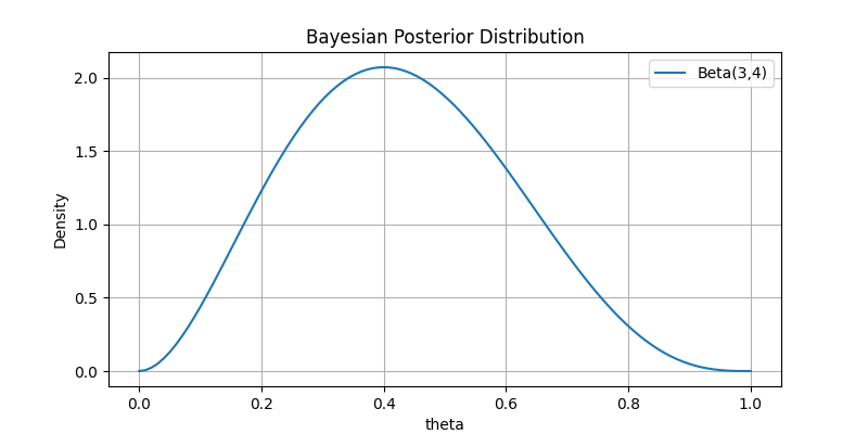
Refer to caption — Figure 1: Posterior distribution of $\theta$ based on observations with 2 up days and 3 down days

As depicted, in such cases, employing a distribution $\mu$ to randomize $\theta$ allows us to capture the variability in environmental performance more effectively. From a modeling perspective, evaluating $\rho_{P_{\theta}}(X)$ under this framework can quantify the DM’s risk preference with respect to the environment through $\rho_{\mu}\circ\rho_{P_{\theta}}(X)$ . Therefore, utilizing $\mu$ as the probability distribution of $\theta$ is more reasonable.

It is possible to express BCR-SOC/MDP as a preference robust SOC/MDP under some specific circumstances. To see this, we consider a BCR where $\rho_{P_{\theta}}=\text{VaR}_{P_{\theta}}^{\alpha}$ for some $\alpha\in(0,1)$ and $\rho_{\mu}=\mathbb{E}_{\mu}$ . The resulting BCR is

\mathbb{E}_{\mu}\circ\text{VaR}_{P_{\theta}}^{\alpha}(X)=\int_{\Theta}\text{VaR}_{P_{\theta}}^{\alpha}(X)\mu(\theta)d\theta.

We will show shortly that the BCR may be expressed as an SRM. Assume, for fixed $\alpha$ , that there exists a bijective function $f:\Theta\to(0,1)$ such that $\text{VaR}_{P_{\theta}}^{\alpha}(X)=\text{VaR}_{P_{\theta^{c}}}^{f(\theta)}(X)$ , where $P_{\theta^{c}}$ is the true probability distribution of $X$ . For fixed $\mu$ and $f$ , let

t=1-f(\theta)\text{ and }\sigma(t)=\mu(f^{-1}(1-t))\cdot\left|\frac{d}{dt}f^{-1}(1-t)\right|.

(3.22)

Then

	$\displaystyle\mathbb{E}_{\mu}\circ\text{VaR}_{P_{\theta}}^{\alpha}(X)$		$\displaystyle=\int_{\Theta}\text{VaR}_{P_{\theta}}^{\alpha}(X)\mu(\theta)d\theta=\int_{\Theta}\text{VaR}_{P_{\theta^{c}}}^{f(\theta)}(X)\mu(\theta)d\theta$
			$\displaystyle=\int_{0}^{1}\text{VaR}_{P_{\theta^{c}}}^{1-t}(X)\sigma(t)dt=\int_{0}^{1}F^{\leftarrow}_{P_{\theta^{c}}}(t)\sigma(t)dt.$

The right-hand side of the equation above is a spectral risk measure, which can be viewed as the weighted average of the randomized $F^{\leftarrow}_{P_{\theta^{c}}}(t)$ . The next example explains how it may work.

Example 7.

Consider a random variable $X$ which follows an exponential distribution parameterized by $\theta$ . It is easy to derive that

\displaystyle\text{VaR}_{P_{\theta}}^{\alpha}(X)=\frac{-\ln\alpha}{\theta}.

Suppose that the true probability distribution of $X$ is $P_{\theta^{c}}$ . By definition, the SRM of $X$ is

\displaystyle M_{\sigma}(X)=\int_{0}^{1}\text{VaR}_{P_{\theta}^{c}}^{1-t}(X)\sigma(t)dt=\int_{0}^{1}\frac{-\ln(1-t)}{\theta^{c}}\sigma(t)dt.

On the other hand, the BCR of $X$ is

\displaystyle\mathbb{E}_{\mu}\circ\text{VaR}_{P_{\theta}}^{\alpha}(X)=\int_{\Theta}\frac{-\ln\alpha}{\theta}\mu(\theta)d\theta.

By setting $f(\theta)=\alpha^{\frac{\theta^{c}}{\theta}}\quad\text{and}\quad t=1-f(\theta)=1-\alpha^{\frac{\theta^{c}}{\theta}}$ , we demonstrate that $\text{VaR}_{P_{\theta}}^{\alpha}(X)=\text{VaR}_{P_{\theta^{c}}}^{1-t}(X).$ Thus, by letting risk spectrum

\displaystyle\sigma(t):=\mu\left(\frac{\theta^{c}\ln\alpha}{\ln(1-t)}\right)\frac{\theta^{c}\ln 1/\alpha}{(1-t)(\ln(1-t))^{2}},

we obtain $\mathbb{E}_{\mu}\circ\text{VaR}_{P_{\theta}}^{\alpha}(X)=M_{\sigma}(X)$ .

Generalizing from this, we consider a generic law invariant coherent risk measure $\rho$ . We know from [61] that $\rho$ can be represented as

\rho(X)=\sup_{\zeta\in\mathfrak{D}}\mathbb{E}_{\zeta}X,

where $\mathfrak{D}$ represents a set of probability density functions.

By adopting a coherent risk measure for the outer risk measure $\rho_{\mu}$ , we have

\rho_{\mu}\circ\text{VaR}_{P_{\theta}}^{\alpha}(X):=\sup_{\tilde{\mu}\in\mathfrak{D}_{\rho_{\mu}}}\int_{\Theta}\text{VaR}_{P_{\theta}}^{\alpha}(X)\tilde{\mu}(\theta)d\theta=\sup_{\sigma\in\mathfrak{A}_{\rho_{\mu}}}\int_{0}^{1}\text{VaR}_{P_{\theta^{c}}}^{1-t}(X)\sigma(t)dt\equiv\sup_{\sigma\in\mathfrak{A}_{\rho_{\mu}}}M_{\sigma}(X),

(3.23)

where $\mathfrak{D}_{\rho_{\mu}}$ is the domain of the Fenchel’s conjugate of $\rho_{\mu}$ (see [61, Theorem 6.5]), and $\mathfrak{A}_{\rho_{\mu}}$ is a set of risk spectra corresponding to $\mathfrak{D}_{\rho_{\mu}}$ based on the one-to-one correspondence between $\mu$ and $\sigma$ as specified in (3.22). The second term in equation (3.23) can be viewed as distributionally robust formulation of $\rho_{\mu}\circ\text{VaR}_{P_{\theta}}^{\alpha}(X)$ , while the third term of the equation is preference robustness of SRM. The robustness in the former is concerned with the ambiguity of the environmental risk represented by $\tilde{\mu}$ whereas the robustness in the latter is concerned with ambiguity of the DM’s preference (represented by $\sigma$ ) associated with the ambiguity in the environmental risk.

Example 8 (Preference robust SOC/MDP).

Let the inner risk measure $\rho_{P_{\theta}}$ be $\text{VaR}_{P_{\theta}}^{\beta}$ and the outer risk measure $\rho_{\mu_{t}}$ be a coherent risk measure. In this case, the objective function of the BCR-SOC/MDP model (3.1) becomes

\min_{\pi}\rho_{\mu_{1}}\circ\text{VaR}_{P_{\theta_{1}}}^{\beta}\left(\mathcal{C}\left(s_{1},a_{1},\xi_{1}\right)+\cdots+\gamma\rho_{\mu_{T-1}}\circ\text{VaR}_{P_{\theta_{T-1}}}^{\beta}\left[\mathcal{C}\left(s_{T-1},a_{T-1},\xi_{T-1}\right)+\gamma\mathcal{C}\left(s_{T}\right)\right]\right).

By virtue of (3.23), we can recast the problem as a preference robust SOC/MDP problem:

\min_{\pi}\sup_{\sigma_{1}\in\mathfrak{A}_{\rho_{\mu_{1}}}}M_{\sigma_{1}}\left[\mathcal{C}\left(s_{1},a_{1},\xi_{1}\right)+\cdots+\gamma\sup_{\sigma_{T-1}\in\mathfrak{A}_{\rho_{\mu_{T-1}}}}M_{\sigma_{T-1}}\left[\mathcal{C}\left(s_{T-1},a_{T-1},\xi_{T-1}\right)+\gamma\mathcal{C}\left(s_{T}\right)\right]\right],

where $\mathfrak{A}_{\rho_{\mu_{t}}}$ , $1\leq t\leq T-1$ , is a set of risk spectra representing the uncertainty of a DM’s risk attitude at episode $t$ . Based on Bayes’ rule, we understand that the updates of $\mu_{t}$ can be established by a continuous process of learning and correction. Therefore, in the corresponding preference robust SOC/MDP model, the DM’s ambiguity set of risk attitude $\mathfrak{A}_{\mu_{t}}$ also evolves continually as the sample data accumulates.

A similar correspondence between BCR-SOC/MDP and preference robust SOC/MDP can be established when the inner risk measure $\rho_{P_{\theta}}$ is $\text{AVaR}_{P_{\theta}}^{\alpha}$ and the outer risk measure $\rho_{\mu}$ is a coherent risk measure. In that case, we can derive a representation akin to the Kusuoka’s representation [36], with Kusuoka’s ambiguity set being induced by $\mu$ . All these will lead to another preference robust SOC/MDP model with Kusuoka’s ambiguity set representing DM’s preference uncertainty.

In summary, the examples discussed above show that the BCR-SOC/MDP model displays the breath of its scope and appropriateness for adaptive and self-learning systems within the realm of risk control. Moreover, by judiciously selecting risk measures and configuring posterior distributions, we can align BCR-SOC/MDP models with preference robust SOC/MDP models.

4 Finite-horizon BCR-SOC/MDP

We now turn to discussing numerical methods for solving (3.1). As with the conventional SOC/MDP models, we need to separate the discussions depending on whether $T<\infty$ and $T=\infty$ . We begin with the former in this section. The finite horizon BCR-SOC/MDP may be regarded as an extension of the risk-neutral MDP [38]. The key step is to derive dynamic recursive equations. In the literature of SOC/MDP and multistage stochastic programming, this relies heavily on interchangeability and the decomposability of the objective function [60]. However, the BCR-SOC/MDP does not require these conditions. The next proposition states this.

Proposition 3.

Let


$\displaystyle V_{T}^{*}\left(s_{T},\mu_{T}\right)$	$\displaystyle=$	$\displaystyle\mathcal{C}_{T}\left(s_{T}\right),\forall\left(s_{T},\mu_{T}\right)\in\mathcal{S}\times\mathcal{D}_{1}^{p},$	(4.1a)
$\displaystyle V_{t}^{*}\left(s_{t},\mu_{t}\right)$	$\displaystyle=$	$\displaystyle\min_{a_{t}\in\mathcal{A}}\rho_{\mu_{t}}\circ\rho_{P_{\theta_{t}}}\left[\mathcal{C}_{t}\left(s_{t},a_{t},\xi_{t}\right)+\gamma V_{t+1}^{*}\left(s_{t+1},\mu_{t+1}\right)\right],$	(4.1b)
		$\displaystyle\qquad\qquad\qquad\qquad\qquad\qquad\forall(s_{t},\mu_{t})\in\mathcal{S}\times\mathcal{D}_{1}^{p},\ t=1,\cdots,T-1,$	(4.1b)

where $s_{t}$ and $\mu_{t}$ satisfy equations (3.1b) and (3.1b), respectively. Let $\mathcal{J}_{T}^{\gamma,*}(s_{1},\mu_{1})$ denote the optimal value of problem (3.1). Under Assumption 1,

\displaystyle\mathcal{J}_{T}^{\gamma,*}(s_{1},\mu_{1})=V_{1}^{*}(s_{1},\mu_{1}).

(4.2)

Moreover, the optimal policy $\pi^{*}=\{\pi_{1}^{*},\cdots,\pi_{T-1}^{*}\}$ corresponding to $\mathcal{J}_{T}^{\gamma,*}(s_{1},\mu_{1})$ exists and can be determined recursively by:

\pi_{t}^{*}\left(s_{t},\mu_{t}\right)\in\arg\min_{a\in\mathcal{A}}\rho_{\mu_{t}}\circ\rho_{P_{\theta_{t}}}\left[\mathcal{C}_{t}\left(s_{t},a_{t},\xi_{t}\right)+\gamma V_{t+1}^{*}\left(s_{t+1},\mu_{t+1}\right)\right].

(4.3)

By analogy with the analysis in [57], Proposition 3 is evident if we treat the state space $\mathcal{S}$ and the posterior distribution space $\mathcal{D}_{1}^{p}$ together as an augmented state space, see [38] for the latter. In alignment with the discussions in [12, 59], the BCR-SOC/MDP formulation (3.1) emphasizes the critical aspect of time consistency within the nested risk function framework. Thus, for the proposed BCR-SOC/MDP model with a finite horizon, we can recursively solve it using a dynamic programming solution procedure such as that outlined in Algorithm 1. We will discuss the details of solving the Bellman equations (4.1a)-(4.1b) in Section 6.

Algorithm 1 Dynamic Programming Method for Finite-horizon BCR-SOC/MDP (3.1).

1: Initialization:

V_{T}^{*}\left(s_{T},\mu_{T}\right)=\mathcal{C}_{T}\left(s_{T}\right)

, for all

\left(s_{T},\mu_{T}\right)\in\mathcal{S}\times\mathcal{D}_{1}^{p}

2: for

t=T-1,T-2,\cdots,1

3: for all

\left(s_{t},\mu_{t}\right)\in\mathcal{S}\times\mathcal{D}_{1}^{p}

4: Solve problem


$\displaystyle\min_{a\in\mathcal{A}}$	$\displaystyle\rho_{\mu_{t}}\circ\rho_{P_{\theta_{t}}}\left[\mathcal{C}_{t}\left(s_{t},a_{t},\xi_{t}\right)+\gamma V_{t+1}^{*}\left(s^{\prime},\mu^{\prime}\right)\right]$	(4.4a)
s.t.	$\displaystyle s^{\prime}=g_{t}(s_{t},a_{t},\xi_{t}),\ \mu^{\prime}=\frac{p\left(\xi_{t}\|\theta\right)\mu_{t}(\theta)}{\int_{\Theta}p\left(\xi_{t}\|\theta\right)\mu_{t}(\theta)d\theta}$	(4.4b)

to obtain an optimal policy

\pi_{t}^{*}\left(s_{t},\mu_{t}\right)

5: Setting

V_{t}^{*}\left(s_{t},\mu_{t}\right):=\rho_{\mu_{t}}\circ\rho_{P_{\theta_{t}}}\left[\mathcal{C}_{t}\left(s_{t},\pi_{t}^{*}\left(s_{t},\mu_{t}\right),\xi_{t}\right)+\gamma V_{t+1}^{*}\left(s^{\prime},\mu^{\prime}\right)\right]

6: end for

7: end for

8: Setting

\mathcal{J}_{T}^{\gamma,*}(s,\mu):=V_{1}^{*}\left(s_{t},\mu_{t}\right)

for all

(s,\mu)\in\mathcal{S}\times\mathcal{D}_{1}^{p}

9: return Optimal policy

\pi^{*}=\{\pi^{*}_{1},\pi^{*}_{1},\cdots,\pi^{*}_{T-1}\}

and the optimal value function

\mathcal{J}_{T}^{\gamma,*}

A key step in Algorithm 1 is to solve problem (4.4) for all $\left(s_{t},\mu_{t}\right)\in\mathcal{S}\times\mathcal{D}_{1}^{p}$ . This is implementable in practice only when $\mathcal{S}\times\mathcal{D}_{1}^{p}$ is a discrete set with finite elements. Moreover, it is often difficult to obtain a closed form of the objective function when $\xi$ is continuously distributed. All these mean that the algorithm is conceptual as it stands. We will return to the issues in Section 6. Another issue is the convexity of problem (4.4). We need to ensure that this is a convex program so that $\pi_{t}^{*}\left(s_{t},\mu_{t}\right)$ is an optimal solution. It is sufficient to ensure that $V_{t+1}^{*}(g_{t}(s_{t},a_{t},\xi_{t}),\mu^{\prime})$ is convex in $a_{t}$ . We address this below. The following assumption is required.

Assumption 2.

For all $\xi_{t}\in\Xi$ , $\mathcal{C}_{t}(s_{t},a_{t},\xi_{t})$ and $g_{t}(s_{t},a_{t},\xi_{t})$ are jointly convex with respect to $(s_{t},a_{t})\in\mathcal{S}\times\mathcal{A}$ .

By comparison with the assumptions in the existing literature (e.g., [22, 63]), Assumption 2 is mild. In these works and in many practical applications, it is typically assumed that $g_{t}$ is affine. Note that the convexity of $g$ is required to ensure that problem (4.1b) is convex which will facilitate numerical solution of the problem. The next proposition states the convexity of problem (4.1b).

Proposition 4.

Let Assumptions 1 and 2 hold. If $\rho_{\mu_{t}}(\cdot)$ and $\rho_{P_{\theta_{t}}}(\cdot)$ are convex risk measures for each episode $t=1,\cdots,T$ , then the following assertions hold.

(i)

Problem (4.1b) is a convex program.

(ii)

If, in addition, $\mathcal{C}_{t}(s_{t},a_{t},\xi_{t})$ and $g_{t}(s_{t},a_{t},\xi_{t})$ are Lipschitz continuous in $s_{t}\in\mathcal{S}$ uniformly for all $a_{t}$ and $\xi_{t}$ with modulus $L_{\mathcal{C}}$ and $L_{g}$ , respectively, then $V^{*}_{t}(s_{t},\mu_{t})$ is Lipschtz continuous in $s_{t}$ , i.e.,

\displaystyle|V_{t}^{*}(s_{t}^{2},\mu_{t})-V_{t}^{*}(s_{t}^{1},\mu_{t})|\leq(L_{\mathcal{C}}+\gamma L_{V_{t+1}}L_{g})\left\|s_{t}^{1}-s_{t}^{2}\right\|,\forall s_{t}^{1},s_{t}^{2}\in{\cal S},

(4.5)

for $t=1,\cdots,T-1$ , where $L_{V_{t}}=\sum_{i=0}^{T-t}(\gamma L_{g})^{i}L_{\mathcal{C}}$ .

(iii)

If, further, $\mathcal{C}_{t}(s_{t},a_{t},\xi_{t})$ and $g_{t}(s_{t},a_{t},\xi_{t})$ are Lipschitz continuous in $a_{t}\in\mathcal{A}$ uniformly for all $s_{t}$ and $\xi_{t}$ , then ${\cal C}_{t}(s_{t},a_{t},\xi_{t})+\gamma V^{*}_{t+1}(s_{t+1},\mu_{t+1})$ is Lipschtz continuous in $a_{t}$ , i.e.,

			$\displaystyle\|\mathcal{C}_{t}\left(s_{t},a_{t}^{1},\xi_{t}\right)+\gamma V^{}_{t+1}\left(g_{t}(s_{t},a_{t}^{1},\xi_{t}),\mu^{\prime}\right)-\mathcal{C}_{t}\left(s_{t},a_{t}^{2},\xi_{t}\right)+\gamma V^{}_{t+1}\left(g_{t}(s_{t},a_{t}^{2},\xi_{t}),\mu^{\prime}\right)\|$		(4.6)
		$\displaystyle\leq$	$\displaystyle(L_{\mathcal{C}}+\gamma L_{V_{t+1}}L_{g})\left\\|a_{t}^{1}-a_{t}^{2}\right\\|,\forall a_{t}^{1},a_{t}^{2}\in{\cal A},$		(4.6)

for $t=1,\cdots,T-1$ .

Proof. Part (i). Due to Assumption 1 (e), it suffices to show that $\rho_{\mu_{t}}\circ\rho_{P_{\theta_{t}}}\left[\mathcal{C}(s_{t},a_{t},\xi_{t})+\gamma V^{*}_{t+1}\left(s_{t+1},\mu_{t+1}\right)\right]$ is jointly convex in $(s_{t},a_{t})$ . Under Assumption 2, the function is jointly convex provided that $V^{*}_{t+1}\left(g_{t}(s_{t},a_{t},\xi_{t}),\mu_{t+1}\right)$ is convex in $a_{t}$ . This is because the BCR is convex and monotone since $\rho_{\mu_{t}}(\cdot)$ and $\rho_{P_{\theta_{t}}}(\cdot)$ are convex risk measures. In what follows, we use backward induction to derive convexity of $V^{*}_{t}$ in $a_{t}$ . Observe that $V_{T}^{*}\left(s_{T},\mu_{T}\right)=\mathcal{C}\left(s_{T}\right),\forall\left(s_{T},\mu_{T}\right)\in\mathcal{S}\times\mathcal{D}_{1}^{p}$ . Thus, the conclusion holds at episode $T$ . Assuming that the convexity holds for episodes from $t+1$ to $T$ , we demonstrate the convexity at episode $t$ . This is evident from (4.1b) in that $V^{*}_{t+1}$ is convex in $s_{t+1}$ and hence $\rho_{\mu_{t}}\circ\rho_{P_{\theta_{t}}}\left[\mathcal{C}_{t}\left(s_{t},a_{t},\xi_{t}\right)+\gamma V_{t+1}^{*}\left(s_{t+1},\mu_{t+1}\right)\right]$ is jointly convex in $(a_{t},s_{t})$ .

Part (ii). We also use backward induction to establish Lipschitz continuity of $V^{*}_{t}(s_{t},\mu_{t})$ in $s_{t}$ . At episode $T$ , the Lipschtz continuity is evident since $V_{T}^{*}\left(s_{T},\mu_{T}\right)=\mathcal{C}\left(s_{T}\right),\forall\left(s_{T},\mu_{T}\right)\in\mathcal{S}\times\mathcal{D}_{1}^{p}$ . Assuming that the Lipschtz continuity holds from episodes $t+1$ to $T$ , we demonstrate that the Lipschitz continuity also holds at episode $t$ . Under the hypothesis of the induction, $V^{*}_{t+1}$ is Lipschtz continuous in $s_{t+1}$ with modulus $L_{V_{t+1}}$ . For any ${s}^{1}_{t},s^{2}_{t}\in\mathcal{S}$ ,

		$\displaystyle\left\|\rho_{\mu_{t}}\circ\rho_{P_{\theta_{t}}}\left[\mathcal{C}_{t}\left(s_{t}^{1},{a}_{t},\xi_{t}\right)+\gamma V^{}_{t+1}\left(g_{t}(s_{t}^{1},a_{t},\xi_{t}),\mu^{\prime}\right)\right]-\rho_{\mu_{t}}\circ\rho_{P_{\theta_{t}}}\left[\mathcal{C}_{t}\left(s_{t}^{2},{a}_{t},\xi_{t}\right)+\gamma V^{}_{t+1}\left(g_{t}(s_{t}^{2},a_{t},\xi_{t}),\mu^{\prime}\right)\right]\right\|$
	$\displaystyle\leq$	$\displaystyle\rho_{\mu_{t}}\circ\rho_{P_{\theta_{t}}}\left\|\mathcal{C}_{t}\left(s_{t}^{1},{a}_{t},\xi_{t}\right)+\gamma V^{}_{t+1}\left(g_{t}(s_{t}^{1},a_{t},\xi_{t}),\mu^{\prime}\right)-\mathcal{C}_{t}\left(s^{2}_{t},{a}_{t},\xi_{t}\right)-\gamma V^{}_{t+1}\left(g_{t}(s_{t}^{2},a_{t},\xi_{t}),\mu^{\prime}\right)\right\|$
	$\displaystyle\leq$	$\displaystyle\rho_{\mu_{t}}\circ\rho_{P_{\theta_{t}}}\left(L_{\mathcal{C}}\left\\|s_{t}^{1}-s_{t}^{2}\right\\|+\gamma L_{V_{t+1}}\left\\|g_{t}(s_{t}^{1},a_{t},\xi_{t})-g_{t}(s_{t}^{2},a_{t},\xi_{t})\right\\|\right)$
	$\displaystyle\leq$	$\displaystyle(L_{\mathcal{C}}+\gamma L_{V_{t+1}}L_{g})\left\\|s_{t}^{1}-s_{t}^{2}\right\\|.$

Thus

		$\displaystyle V_{t}^{}(s_{t}^{1},\mu_{t})-V_{t}^{}(s_{t}^{2},\mu_{t})$
	$\displaystyle\leq$	$\displaystyle\sup_{a_{t}\in\mathcal{A}}\left\|\rho_{\mu_{t}}\circ\rho_{P_{\theta_{t}}}[\mathcal{C}_{t}\left(s_{t}^{1},a_{t},\xi_{t}\right)+\gamma V^{}_{t+1}\left(g_{t}(s_{t}^{1},{a}_{t},\xi_{t}),\mu^{\prime}\right)]-\rho_{\mu_{t}}\circ\rho_{P_{\theta_{t}}}[\mathcal{C}_{t}\left(s^{2}_{t},{a}_{t},\xi_{t}\right)-\gamma V^{}_{t+1}\left(g_{t}(s_{t}^{2},a_{t},\xi_{t}),\mu^{\prime}\right)]\right\|$
	$\displaystyle\leq$	$\displaystyle(L_{\mathcal{C}}+\gamma L_{V_{t+1}}L_{g})\left\\|s_{t}^{1}-s_{t}^{2}\right\\|.$

A similar conclusion can be derived by swapping the positions of $V_{t}^{*}(s_{t}^{1},\mu_{t})$ and $V_{t}^{*}(s_{t}^{2},\mu_{t})$ . Therefore, we have

|V_{t}^{*}(s_{t}^{2},\mu_{t})-V_{t}^{*}(s_{t}^{1},\mu_{t})|\leq(L_{\mathcal{C}}+\gamma L_{V_{t+1}}L_{g})\left\|s_{t}^{1}-s_{t}^{2}\right\|.

This deduction confirms by mathematical induction that the Lipschitz continuity property holds for all episodes.

Part (iii). For any ${a}^{1}_{t},a^{2}_{t}\in\mathcal{A}$ , we have:

		$\displaystyle\|\mathcal{C}_{t}\left(s_{t},a_{t}^{1},\xi_{t}\right)+\gamma V^{}_{t+1}\left(g_{t}(s_{t},a_{t}^{1},\xi_{t}),\mu^{\prime}\right)-\mathcal{C}_{t}\left(s_{t},a_{t}^{2},\xi_{t}\right)+\gamma V^{}_{t+1}\left(g_{t}(s_{t},a_{t}^{2},\xi_{t}),\mu^{\prime}\right)\|$
	$\displaystyle\leq$	$\displaystyle L_{\mathcal{C}}\left\\|a_{t}^{1}-a_{t}^{2}\right\\|+\gamma L_{V_{t+1}}\|\|g_{t}(s_{t},a_{t}^{1},\xi_{t})-g_{t}(s_{t},a_{t}^{2},\xi_{t})\|\|$
	$\displaystyle\leq$	$\displaystyle(L_{\mathcal{C}}+\gamma L_{V_{t+1}}L_{g})\left\\|a_{t}^{1}-a_{t}^{2}\right\\|$

for $t=1,\cdots,T-1$ . $\Box$

5 Infinite-horizon BCR-SOC/MDP

In this section, we move on to discuss the BCR-SOC/MDP problem (3.1) with infinite-horizon, i.e., $T=\infty$ . We start with the following assumption.

Assumption 3.

Consider problem (3.1). (a) The transition dynamics are time-invariant, i.e., $g_{t}(s,a,\xi)\equiv g(s,a,\xi)$ and $\mathcal{C}_{t}(s,a,\xi)\equiv\mathcal{C}(s,a,\xi)$ for all $t$ . (b) For all $(s,a,\xi)\in\mathcal{S}\times\mathcal{A}\times\Xi$ , the absolute value of the cost function $|\mathcal{C}(s,a,\xi)|$ is bounded by a constant $\bar{\mathcal{C}}$ . (c) The discount factor $\gamma\in(0,1)$ .

Under Assumption 3, we can formulate the BCR-SOC/MDP model (3.1) as follows:


$\displaystyle\min_{\pi}$	$\displaystyle\mathcal{J}_{\infty}^{\gamma}(\pi,s_{1},\mu_{1}):=\rho_{\mu_{1}}\circ\rho_{P_{\theta_{1}}}\left[\mathcal{C}\left(s_{1},a_{1},\xi_{1}\right)+\cdots+\gamma\rho_{\mu_{t}}\circ\rho_{P_{\theta_{t}}}\left[\mathcal{C}\left(s_{t},a_{t},\xi_{t}\right)+\cdots\right]\right]$	(5.1a)
s.t.	$\displaystyle s_{t+1}=g\left(s_{t},a_{t},\xi_{t}\right),\ a_{t}=\pi(s_{t},\mu_{t}),\ t=1,2,\cdots;$	(5.1c)
	$\displaystyle\mu_{t+1}(\theta)=\frac{p\left(\xi_{t}\|\theta\right)\mu_{t}(\theta)}{\int_{\Theta}p\left(\xi_{t}\|\theta\right)\mu_{t}(\theta)d\theta},\ t=1,2,\cdots.$	(5.1c)

We use $\mathcal{J}_{\infty}^{\gamma,*}$ to denote the optimal value of problem (5.1). Given the boundness of the cost function $\mathcal{C}(s,a,\xi)$ , it follows that the value function $\mathcal{J}_{\infty}^{\gamma,*}$ is also bounded, i.e.,

||\mathcal{J}_{\infty}^{\gamma,*}||_{\infty}:=\sup_{(s,\mu)\in\mathcal{S}\times\mathcal{D}^{0}_{1}}|\mathcal{J}_{\infty}^{\gamma,*}(s,\mu)|\leq\frac{\bar{\mathcal{C}}}{1-\gamma}.

5.1 Bellman equation and optimality

It is challenging to solve the infinite-horizon BCR-SOC/MDP problem (5.1). A standard approach is to use the Bellman equation to develop an iterative scheme analogous to those used in the existing SOC/MDP models (e.g., [22, 63, 82]). We begin by defining the Bellman equation of (5.1).

Definition 1 (Deterministic Bellman operator).

Let $\mathfrak{B}(\mathcal{S},\mathcal{D}_{1}^{0})$ denote the space of real-valued bounded measurable functions on $\mathcal{S}\times\mathcal{D}_{1}^{0}$ . For any value function $V\in\mathfrak{B}(\mathcal{S},\mathcal{D}_{1}^{0})$ , define the deterministic operator $\mathcal{T}:\mathfrak{B}(\mathcal{S},\mathcal{D}_{1}^{0})\rightarrow\mathfrak{B}(\mathcal{S},\mathcal{D}_{1}^{0})$ as follows:

(\mathcal{T}V)(s,\mu)=\min_{a\in\mathcal{A}}\rho_{\mu}\circ\rho_{P_{\theta}}\left(\mathcal{C}(s,a,\xi)+\gamma V\left(s^{\prime},\mu^{\prime}\right)\right)\text{ for all}\;\;s,\mu

(5.2)

and operator $\mathcal{T}^{\pi}:\mathfrak{B}(\mathcal{S},\mathcal{D}_{1}^{0})\rightarrow\mathfrak{B}(\mathcal{S},\mathcal{D}_{1}^{0})$ for a given $\pi$ :

\displaystyle\left(\mathcal{T}^{\pi}V\right)(s,\mu)=\rho_{\mu}\circ\rho_{P_{\theta}}\left(\mathcal{C}(s,\pi(s,\mu),\xi)+\gamma V\left(s^{\prime},\mu^{\prime}\right)\right).

(5.3)

The dynamic programming formulation integrated into the Bellman operator ensures that risk factors are effectively incorporated into the decision-making process. This approach accounts systematically for both epistemic and aleatoric uncertainties, which are crucial when determining the optimal policy at each decision point. In the Bellman equation presented above, the random variable $\xi$ serves as a general representation of the stochastic input in each decision episode. This simplification helps to maintain the recursive structure of the model without the need to explicitly track time indices for the random variables.

Model (5.1) and the Bellman equation (5.2) assume deterministic policies, but the rationale behind this set-up has not yet been explained fully. The next lemma states that optimizing over randomized policies is essentially equivalent to optimizing over deterministic ones. The latter will simplify the decision problem and improve computational efficiency.

Lemma 2.

The deterministic Bellman operator is equivalent to the random Bellman operator, i.e.,

	$\displaystyle(\mathcal{T}V)(s,\mu)$	$\displaystyle=\min_{a\in\mathcal{A}}\rho_{\mu}\circ\rho_{P_{\theta}}\left(\mathcal{C}(s,a,\xi)+\gamma V\left(s^{\prime},\mu^{\prime}\right)\right)$
		$\displaystyle=\inf_{\pi\in\Pi^{R}}\mathbb{E}_{a\sim\pi(s,\mu)}\left[\rho_{\mu}\circ\rho_{P_{\theta}}\left(\mathcal{C}(s,a,\xi)+\gamma V\left(s^{\prime},\mu^{\prime}\right)\right)\right],$

where $\Pi^{R}$ denotes the set of all randomized policies.

Proof. Denote an arbitrary randomized policy $\pi$ by $\pi(s,\mu,a)=P(\pi(s,\mu)=a)$ . For any value function $V$ , we have

\inf_{a\in\mathcal{A}}\rho_{\mu}\circ\rho_{\theta}\left[\mathcal{C}(s,a,\xi)+\gamma V\left(s^{\prime},\mu^{\prime}\right)\right]\leq\int_{a\in\mathcal{A}}\rho_{\mu}\circ\rho_{\theta}\left[\mathcal{C}(s,a,\xi)+\gamma V\left(s^{\prime},\mu^{\prime}\right)\right]dP.

Hence,

(\mathcal{T}V)(s,\mu)=\min_{a\in\mathcal{A}}\rho_{\mu}\circ\rho_{P_{\theta}}\left[\mathcal{C}(s,a,\xi)+\gamma V\left(s^{\prime},\mu^{\prime}\right)\right]\leq\inf_{\pi\in\Pi^{R}}\mathbb{E}_{a\sim\pi(s,\mu)}\left[\rho_{\mu}\circ\rho_{P_{\theta}}\left[\mathcal{C}(s,a,\xi)+\gamma V\left(s^{\prime},\mu^{\prime}\right)\right]\right].

The reverse is straightforward, as a deterministic policy is a special case of a randomized policy. $\Box$

The proof leverages an arbitrary randomized policy $\pi$ to demonstrate that the deterministic Bellman operator indeed corresponds to the random Bellman operator, thereby justifying our focus on deterministic policies. This simplification, however, does not preclude the extension of our analysis to randomized policies. In what follows, we demonstrate that the optimal value function $\mathcal{J}_{\infty}^{\gamma,*}$ of BCR-SOC/MDP problem (5.1) is the unique fixed point of operator $\mathcal{T}$ . Specifically,

\displaystyle\mathcal{T}\mathcal{J}_{\infty}^{\gamma,*}(s,\mu)=\mathcal{J}_{\infty}^{\gamma,*}(s,\mu),\forall(s,\mu)\in{\cal S}\times{\cal D}_{1}^{0}.

(5.4)

To this end, we derive an intermediate result to ensure that the Bellman operators defined in Definition 1 are monotonic and contractive.

Lemma 3 (Monotonicity and contraction).

Let $\mathcal{T}$ and $\mathcal{T}^{\pi}$ be defined as in (5.2) and (5.3). The following assertions hold.

(i)

Both $\mathcal{T}$ and $\mathcal{T}^{\pi}$ are monotonic, i.e., $V\leq V^{\prime}$ implies that $\mathcal{T}V\leq\mathcal{T}V^{\prime}$ and $\mathcal{T}^{\pi}V\leq\mathcal{T}^{\pi}V^{\prime}$ .

(ii)

For any measurable functions $f_{i}:\Theta\to\mathbb{R}$ and $g_{i}:\Xi\to\mathbb{R}$ , $i=1,2$ ,

\displaystyle|\rho_{\mu}(f_{1}(\theta))-\rho_{\mu}(f_{2}(\theta))|\leq\|f_{1}(\theta)-f_{2}(\theta)\|_{\theta,\infty}

(5.5)

and

\displaystyle|\rho_{P_{\theta}}(g_{1}(\xi))-\rho_{P_{\theta}}(g_{2}(\xi))|\leq\|g_{1}(\xi)-g_{2}(\xi)\|_{\xi,\infty},

(5.6)

where $\|\cdot\|_{\theta,\infty}$ is the sup-norm under probability measure $\mu$ and $\|\cdot\|_{\xi,\infty}$ is the sup-norm under probability measure $P_{\theta}$ .

(iii)

The operators $\mathcal{T}$ and $\mathcal{T}^{\pi}$ are $\gamma$ contractive with respect to the $\|\cdot\|_{\infty}$ norm. That is, for any bounded value functions $V,V^{\prime}\in\mathfrak{B}(\mathcal{S},\mathcal{D}_{1}^{0})$ , we have

\left\|\mathcal{T}V-\mathcal{T}V^{\prime}\right\|_{\infty}\leq\gamma\left\|V-V^{\prime}\right\|_{\infty}\text{ and }\left\|\mathcal{T}^{\pi}V-\mathcal{T}^{\pi}V^{\prime}\right\|_{\infty}\leq\gamma\left\|V-V^{\prime}\right\|_{\infty}.

Proof. Part (i). By definition

\left(\mathcal{T}^{\pi}V\right)(s,\mu)=\rho_{\mu}\circ\rho_{P_{\theta}}\left[\mathcal{C}(s,\pi(s,\mu),\xi)+\gamma V\left(s^{\prime},\mu^{\prime}\right)\right].

If two value functions $V$ and $V^{\prime}$ satisfy $V\left(s^{\prime},\mu^{\prime}\right)\leq V^{\prime}\left(s^{\prime},\mu^{\prime}\right)$ for all $s^{\prime}\in\mathcal{S}$ and $\mu^{\prime}\in\mathcal{D}_{1}^{0}$ , then we can deduce $\left(\mathcal{T}^{\pi}V\right)(s,\mu)\leq\left(\mathcal{T}^{\pi}V^{\prime}\right)(s,\mu)$ given the monotonicity of the composite risk measure. The same argument applies to $\mathcal{T}$ .

Part (ii). The inequalities are known as non-expansive properties of a risk measure satisfying translation invariance, see (2.10).

Part (iii). For any $\varepsilon>0$ , there exists a deterministic policy $\pi$ , such that for any $(s,\mu)\in\mathcal{S}\times\mathcal{D}_{1}^{0}$ ,

(\mathcal{T}V^{\prime})(s,\mu)\geq\rho_{\mu}\circ\rho_{P_{\theta}}\left[\mathcal{C}(s,\pi(s,\mu),\xi)+\gamma V^{\prime}\left(s^{\prime},\mu^{\prime}\right)\right]-\varepsilon.

Consequently, we have

		$\displaystyle(\mathcal{T}V)(s,\mu)-(\mathcal{T}V^{\prime})(s,\mu)$
	$\displaystyle\leq$	$\displaystyle\rho_{\mu}\circ\rho_{P_{\theta}}\left[\mathcal{C}(s,\pi(s,\mu),\xi)+\gamma V\left(s^{\prime},\mu^{\prime}\right)\right]-\rho_{\mu}\circ\rho_{P_{\theta}}\left[\mathcal{C}(s,\pi(s,\mu),\xi)+\gamma V^{\prime}\left(s^{\prime},\mu^{\prime}\right)\right]+\varepsilon$
	$\displaystyle\leq$	$\displaystyle\gamma\left(\rho_{\mu}\circ\rho_{P_{\theta}}\left[V\left(s^{\prime},\mu^{\prime}\right)\right]-\rho_{\mu}\circ\rho_{P_{\theta}}\left[V^{\prime}\left(s^{\prime},\mu^{\prime}\right)\right]\right)+\varepsilon$
	$\displaystyle\leq$	$\displaystyle\gamma\left\\|\rho_{P_{\theta}}\left[V\left(s^{\prime},\mu^{\prime}\right)\right]-\rho_{P_{\theta}}\left[V^{\prime}\left(s^{\prime},\mu^{\prime}\right)\right]\right\\|_{\theta,\infty}+\varepsilon$
	$\displaystyle\leq$	$\displaystyle\gamma\left\\|\left\\|V\left(s^{\prime},\mu^{\prime}\right)-V^{\prime}\left(s^{\prime},\mu^{\prime}\right)\right\\|_{\xi,\infty}\right\\|_{\theta,\infty}+\varepsilon$
	$\displaystyle\leq$	$\displaystyle\gamma\\|V-V^{\prime}\\|_{\infty}+\varepsilon.$

Since an arbitrarily small $\varepsilon$ can be chosen, this implies that $\left\|(\mathcal{T}V)-(\mathcal{T}V^{\prime})\right\|_{\infty}\leq\gamma\|V-V^{\prime}\|_{\infty}$ . Switching the positions of $V$ and $V^{\prime}$ , we obtain the desired result for $\mathcal{T}$ . The proof of $\mathcal{T}^{\pi}$ is analogous to that for $\mathcal{T}$ . $\Box$

We are now ready to present the main result of this section which states the existence of a unique solution to Bellman equation (5.4) and the solution coinciding with the optimal value of the infinite BCR-SOC/MDP (5.1).

Theorem 1.

Consider Bellman equation (5.4). The following assertions hold.

(i)

Equation (5.4) has a unique value function $V^{*}$ . Moreover, for any value function $V\in\mathfrak{B}(\mathcal{S},\mathcal{D}_{1}^{0})$ , if $V\geq\mathcal{T}V$ , then $V\geq V^{*}$ , and, if $V\leq\mathcal{T}V$ , then $V\leq V^{*}$ .
(ii)

The optimal value of problem (5.1), $\mathcal{J}_{\infty}^{\gamma,*}$ , is the unique solution to that of (5.4), i.e.,

$\mathcal{J}_{\infty}^{\gamma,*}(s,\mu)\equiv V^{*}(s,\mu),\ \forall(s,\mu)\in\mathcal{S}\times\mathcal{D}_{1}^{0}.$

Proof. Part (i). Since $\mathcal{T}$ is contractive, the existence and uniqueness of the optimal function $V^{*}$ follows directly from the Banach fixed-point theorem. We prove the other two arguments below. Consider any policy $\pi$ such that

V\geq\mathcal{T}^{\pi}V.

(5.7)

Such a policy $\pi$ always exists since we can choose $\pi$ such that $\mathcal{T}^{\pi}V=\mathcal{T}V$ . By applying $\mathcal{T}^{\pi}$ iteratively to both sides of (5.7) and invoking the monotonicity property from Lemma 3, we deduce that $V\geq\left(\mathcal{T}^{\pi}\right)^{n}V$ for all $n\in\mathbb{N}^{+}$ . Here, $\left(\mathcal{T}^{\pi}\right)^{n}V$ represents the accumulated risk value over a finite horizon with the stationary policy $\pi$ and the terminal value function $V$ . Specifically,

		$\displaystyle\left(\mathcal{T}^{\pi}\right)^{n}V$
		$\displaystyle=\rho_{\mu_{1}}\circ\rho_{P_{\theta_{1}}}\left[\mathcal{C}\left(s_{1},a_{1},\xi_{1}\right)+\gamma\rho_{\mu_{2}}\circ\rho_{P_{\theta_{2}}}\left[\mathcal{C}\left(s_{2},a_{2},\xi_{2}\right)+\cdots+\gamma\rho_{\mu_{n}}\circ\rho_{P_{\theta_{n}}}\left[\mathcal{C}\left(s_{n},a_{n},\xi_{n}\right)+\gamma V\left(s_{n+1},\mu_{n+1}\right)\right]\right]\right]$
		$\displaystyle\geq\rho_{\mu_{1}}\circ\rho_{P_{\theta_{1}}}\left[\mathcal{C}\left(s_{1},a_{1},\xi_{1}\right)+\gamma\rho_{\mu_{2}}\circ\rho_{P_{\theta_{2}}}\left[\mathcal{C}\left(s_{2},a_{2},\xi_{2}\right)+\cdots+\gamma\rho_{\mu_{n}}\circ\rho_{P_{\theta_{n}}}\left[\mathcal{C}\left(s_{n},a_{n},\xi_{n}\right)\right]\right]\right].$

As $n$ tends to infinity, the sequence at right-hand side converges to the value function under the policy $\pi$ . Since $V^{*}$ is defined as the minimum over all such policies, then $V\geq V^{*}$ .

Next, consider a finite horizon BCR-SOC/MDP with the risk value at last episode defined as $V\left(s_{t+1},\mu_{t+1}\right)$ . It follows that:

\rho_{\mu_{t}}\circ\rho_{P_{\theta_{t}}}\left[{\cal C}\left(s_{t},a_{t},\xi_{t}\right)+\gamma V\left(s_{t+1},\mu_{t+1}\right)\right]\geq(\mathcal{T}V)\left(s_{t},\mu_{t}\right)\geq V\left(s_{t},\mu_{t}\right).

Therefore, we can deduce

		$\displaystyle\rho_{\mu_{1}}\circ\rho_{P_{\theta_{1}}}\left[\mathcal{C}\left(s_{1},a_{1},\xi_{1}\right)+\gamma\rho_{\mu_{2}}\circ\rho_{P_{\theta_{2}}}\left[\mathcal{C}\left(s_{2},a_{2},\xi_{2}\right)+\cdots+\gamma V\left(s_{t+1},\mu_{t+1}\right)\right]\right]$
	$\displaystyle\geq$	$\displaystyle\rho_{\mu_{1}}\circ\rho_{P_{\theta_{1}}}\left[\mathcal{C}\left(s_{1},a_{1},\xi_{1}\right)+\gamma\rho_{\mu_{2}}\circ\rho_{P_{\theta_{2}}}\left[\mathcal{C}\left(s_{2},a_{2},\xi_{2}\right)+\cdots+\gamma V\left(s_{t},\mu_{t}\right)\right]\right].$

By setting $s_{1}=s$ and $\mu_{1}=\mu$ , we have

\rho_{\mu_{1}}\circ\rho_{P_{\theta_{1}}}\left[\mathcal{C}\left(s_{1},a_{1},\xi_{1}\right)+\gamma\rho_{\mu_{2}}\circ\rho_{P_{\theta_{2}}}\left[\mathcal{C}\left(s_{2},a_{2},\xi_{2}\right)+\cdots+\gamma V\left(s_{t+1},\mu_{t+1}\right)\right]\right]\geq V(s,\mu).

Let $V_{\max}$ be an upper bound on $|V(s,\mu)|,\forall s\in\mathcal{S},\mu\in\mathcal{D}_{1}^{0}$ , we have

\rho_{\mu_{1}}\circ\rho_{P_{\theta_{1}}}\left[\mathcal{C}\left(s_{1},a_{1},\xi_{1}\right)+\gamma\rho_{\mu_{2}}\circ\rho_{P_{\theta_{2}}}\left[\mathcal{C}\left(s_{2},a_{2},\xi_{2}\right)+\cdots+\gamma\rho_{\mu_{t}}\circ\rho_{P_{\theta_{t}}}\mathcal{C}\left(s_{t},a_{t},\xi_{t}\right)\right]\right]\geq V(s,\mu)-V_{\max}\gamma^{t}.

As $t\rightarrow\infty$ , the left-hand side of the inequality converges to the value function under the policy $\pi$ . The infimum over all policy $\pi$ is bounded from below by $V(s,\mu)$ , leading to the conclusion that $V^{*}\geq V$ .

Part (ii). To begin, with the definition of $\mathcal{J}_{T}^{\gamma}(\pi,s,\mu)$ , for any horizon $T$ , state $s$ , $\mu$ and policy $\pi$ , we have that

\mathcal{J}_{T}^{\gamma,*}(s,\mu)\leq\mathcal{J}_{T}^{\gamma}(\pi,s,\mu)\leq\mathcal{J}_{\infty}^{\gamma}(\pi,s,\mu).

Therefore,

\mathcal{J}_{T}^{\gamma,*}(s,\mu)\leq\mathcal{J}_{\infty}^{\gamma,*}(s,\mu).

Given the monotone property of Bellman operator $\mathcal{T}$ , $\mathcal{J}_{T}^{\gamma,*}(s,\mu)$ forms a nondecreasing sequence which implies that $\lim_{T\to\infty}\mathcal{J}_{T}^{\gamma,*}=V^{*}.$

Hence, to complete the proof, it only remains to show that $V^{*}\geq\mathcal{J}_{\infty}^{\gamma,*}$ . Consider any policy $\pi$ such that $V^{*}\geq(\mathcal{T}^{\pi})V^{*}$ . By iterating this inequality, for all $n\geq 1$ and $(s,\mu)\in\mathcal{S}\times\mathcal{D}_{1}^{0}$ , we obtain:

\displaystyle V^{*}(s,\mu)\geq\rho_{\mu_{1}}\circ\rho_{P_{\theta_{1}}}\left[\mathcal{C}\left(s_{1},a_{1},\xi_{1}\right)+\gamma\rho_{\mu_{2}}\circ\rho_{P_{\theta_{2}}}\left[\mathcal{C}\left(s_{2},a_{2},\xi_{2}\right)+\cdots+\gamma\rho_{\mu_{n}}\circ\rho_{P_{\theta_{n}}}\left[\mathcal{C}\left(s_{n},a_{n},\xi_{n}\right)\right]\right]\right].

Letting $n\to\infty$ , it follows that for all $(s,\mu)\in\mathcal{S}\times\mathcal{D}_{1}^{0}$ ,

V^{*}(s,\mu)\geq\mathcal{J}_{\infty}^{\gamma}(\pi,s,\mu)\geq\mathcal{J}_{\infty}^{\gamma,*}(s,\mu).

Therefore, combining this result with Part (i) of Theorem 1, we conclude that $\mathcal{J}_{\infty}^{\gamma,*}\equiv V^{*}$ satisfies the Bellman equation $\mathcal{J}_{\infty}^{\gamma,*}=\mathcal{T}\mathcal{J}_{\infty}^{\gamma,*}$ . $\Box$

5.2 Asymptotic convergence

Let $V^{*}$ be defined as in Theorem 1 and $P_{\theta^{c}}$ be defined in Section 2. Define

V^{*}(s,\delta_{\theta^{c}})=\min_{a\in\mathcal{A}}\rho_{P_{\theta^{c}}}\left[\mathcal{C}(s,a,\xi)+\gamma V^{*}\left(s^{\prime},\delta_{\theta^{c}}\right)\right]

(5.8)

and

\pi^{*}(s,\delta_{\theta^{c}})\in\arg\min_{a\in\mathcal{A}}\rho_{P_{\theta^{c}}}\left[\mathcal{C}(s,a,\xi)+\gamma V^{*}\left(s^{\prime},\delta_{\theta^{c}}\right)\right].

(5.9)

For $t=1,2,\cdots$ , let $\mu_{t}$ be defined as in (5.1c). Define

V^{*}(s,\mu_{t})=\min_{a\in\mathcal{A}}\rho_{\mu_{t}}\circ\rho_{P_{\theta}}\left[\mathcal{C}(s,a,\xi)+\gamma V^{*}\left(s^{\prime},\mu_{t+1}\right)\right]

(5.10)

and

\pi^{*}(s,\mu_{t})\in\arg\min_{a\in\mathcal{A}}\rho_{\mu_{t}}\circ\rho_{P_{\theta}}\left[\mathcal{C}(s,a,\xi)+\gamma V^{*}\left(s^{\prime},\mu_{t+1}\right)\right].

(5.11)

In this section, we investigate the convergence of $V^{*}(s,\mu_{t})$ to $V^{*}(s,\delta_{\theta^{c}})$ and $\pi^{*}(s,\mu_{t})$ to $\pi^{*}(s,\delta_{\theta^{c}})$ as $t\to\infty$ . The rationale behind the convergence analysis is that in the infinite-horizon Markov decision making process, the DM and the environment interact continuously, allowing the DM to acquire gradually an infinite amount of information about the true environment (represented by the true probability distribution of $\xi$ ). As information or data accumulates, the DM’s understanding of the environment improves continuously, diminishing the uncertainty of $\theta$ . This raises a question as to whether the optimal value $V^{*}(s,\mu_{t})$ and the optimal policy $\pi^{*}(s,\mu_{t})$ , obtained from solving the BCR-SOC/MDP model (5.1), converge to their respective true optimal counterparts, $V^{*}(s,\delta_{\theta^{c}})$ and $\pi^{*}(s,\delta_{\theta^{c}})$ as the data set expands. The first step is to derive weak convergence of $\mu_{t}$ to $\delta_{\theta^{c}}$ . To this end, we need the following assumption.

Assumption 4.

Let $m_{t}$ and $v_{t}$ denote the posterior mean and variance with respect to $\mu_{t}$ . As $t$ tends to infinity, $v_{t}\to 0$ and $m_{t}\to\theta^{c}$ almost surely (a.s.).

This assumption indicates that as the sequence $\bm{\xi}^{t}$ expands with the increase of $t$ , more observations of $\xi$ are gathered. Consequently, the Bayesian posterior distribution will increasingly concentrate around $\theta^{c}$ , eventually reducing to a Dirac function centered at $\theta^{c}$ . The following example illustrates that this assumption is reasonable.

Example 9.

Consider the inventory control problem, as proposed in [38]. Based on experience and relevant expertise, a warehouse manager believes that the customer demand follows a Poisson distribution with parameter $\theta^{c}$ . The prior distribution $\mu_{0}$ is modeled as a $\operatorname{Gamma}(a,b)$ distribution, which, because of its conjugate nature with respect to the Poisson distribution, ensures that the posterior distribution $\mu_{t}$ of $\theta$ remains within the Gamma distribution family with updated parameters $\left(a_{t},b_{t}\right)$ . Here, $a_{t}=a+t\bar{\xi}$ , $\bar{\xi}=\frac{\sum_{i=1}^{t}\xi_{i}}{t}$ and $b_{t}=b+t$ . Therefore, the posterior mean and variance can easily be calculated as

m_{t}=\frac{a+t\bar{\xi}}{b+t}\quad\text{ and }\quad v_{t}=\frac{a+t\bar{\xi}}{(b+t)^{2}}.

By the law of large numbers, $\bar{\xi}\rightarrow\theta^{c}$ a.s. under the true distribution $P_{\theta^{c}}$ . From this, it follows immediately that $v_{t}\rightarrow 0$ and $m_{t}\rightarrow\theta^{c}$ almost surely, thereby satisfying Assumption 4. Further, since the convergence rate of $\bar{\xi}$ is $O(t^{-1/2})$ , we have

\lim_{t\to\infty}{t}\max\{(m_{t}-\theta^{c})^{2},v_{t}\}=\theta^{c},

which verifies the conditions required in Theorem 3 presented below.

Proposition 5.

Under Assumption 4, for any $\varepsilon>0$ , we have that

\lim_{t\to\infty}\int_{\theta\in\mathbb{B}(\theta^{c},\varepsilon)}\mu_{t}(\theta)d\theta=1,\ \text{a.s.}

(5.12)

where $\mathbb{B}(\theta^{c},\varepsilon):=\{\theta:|\theta-\theta^{c}|\leq\varepsilon\}$ denotes the neighborhood around $\theta^{c}$ .

In [63], this result is called Bayesian consistency, see Assumption 3.2 there. As shown in [27], it follows by Markov’s inequality that

\int_{\theta\in\mathbb{B}(\theta^{c},\varepsilon)}\mu_{t}(\theta)d\theta\geq 1-\frac{v_{t}+(m_{t}-\theta^{c})^{2}}{\varepsilon^{2}}.

(5.13)

Therefore, the Bayesian consistency as stated in (5.12) is achieved under Assumption 4.

Lemma 4.

Under Assumption 4, $\mu_{t}$ converges weakly to the Dirac measure $\delta_{\theta^{c}}$ , i.e.,

\displaystyle\lim_{t\to\infty}\int_{\Theta}h(\theta)\mu_{t}(\theta)d\theta=h({\theta^{c}})

(5.14)

for any bounded and continuous function $h$ . Moreover, $\rho_{\mu_{t}}(h(\theta))$ converges to $\rho_{\delta_{\theta^{c}}}\left(h({\theta})\right)=h({\theta^{c}})$ as $t$ goes to infinity.

Proof. The result is similar to [62, Lemma 3.2], here we give a proof for completeness. For any $\epsilon>0$ , decompose the integral as follows:

\displaystyle\int_{\Theta}h(\theta)\mu_{t}(\theta)d\theta=\int_{\mathbb{B}(\theta^{c},\varepsilon)}h(\theta)\mu_{t}(\theta)d\theta+\int_{\Theta\setminus\mathbb{B}(\theta^{c},\varepsilon)}h(\theta)\mu_{t}(\theta)d\theta,

(5.15)

Since $h$ is continuous, for any $\epsilon>0$ , there exists an $\varepsilon_{0}>0$ such that for all $\varepsilon\leq\varepsilon_{0}$ and $\theta\in\mathbb{B}(\theta^{c},\varepsilon)$ , $|h(\theta)-h(\theta^{c})|<\epsilon$ . Consequently, we have

\left|\int_{\mathbb{B}(\theta^{c},\varepsilon)}h(\theta)\mu_{t}(\theta)d\theta-\int_{\mathbb{B}(\theta^{c},\varepsilon)}h(\theta^{c})\mu_{t}(\theta)d\theta\right|<\epsilon\int_{\mathbb{B}(\theta^{c},\varepsilon)}\mu_{t}(\theta)d\theta.

Since $\int_{\mathbb{B}(\theta^{c},\varepsilon)}\mu_{t}(\theta)d\theta\leq 1$ , this implies

\displaystyle\left|\int_{\mathbb{B}(\theta^{c},\varepsilon)}h(\theta)\mu_{t}(\theta)d\theta-\int_{\mathbb{B}(\theta^{c},\varepsilon)}h(\theta^{c})\mu_{t}(\theta)d\theta\right|<\epsilon.

(5.16)

On the other hand, since $h$ is bounded, then there exists a constant $M>0$ such that $|h(\theta)|\leq M$ for all $\theta\in\Theta$ . Together with (5.12), we have

\displaystyle\left|\int_{\Theta\setminus\mathbb{B}(\theta^{c},\varepsilon)}h(\theta)\mu_{t}(\theta)d\theta-\int_{\Theta\setminus\mathbb{B}(\theta^{c},\varepsilon)}h(\theta^{c})\mu_{t}(\theta)d\theta\right|\leq 2M\int_{\Theta\setminus\mathbb{B}(\theta^{c},\varepsilon)}\mu_{t}(\theta)d\theta\to 0

(5.17)

as $t\to\infty$ . Combining (5.15)-(5.17), we obtain

		$\displaystyle\left\|\int_{\Theta}h(\theta)\mu_{t}(\theta)d\theta-h(\theta^{c})\right\|$
	$\displaystyle\leq$	$\displaystyle\left\|\int_{\mathbb{B}(\theta^{c},\varepsilon)}h(\theta)\mu_{t}(\theta)d\theta-h(\theta^{c})\int_{\mathbb{B}(\theta^{c},\varepsilon)}\mu_{t}(\theta)d\theta\right\|+\left\|\int_{\Theta\setminus\mathbb{B}(\theta^{c},\varepsilon)}h(\theta)\mu_{t}(\theta)d\theta-\int_{\Theta\setminus\mathbb{B}(\theta^{c},\varepsilon)}h(\theta^{c})\mu_{t}(\theta)d\theta\right\|$
	$\displaystyle\leq$	$\displaystyle\epsilon+2M\int_{\Theta\setminus\mathbb{B}(\theta^{c},\varepsilon)}\mu_{t}(\theta)d\theta.$

Since $\epsilon$ can be arbitrarily small, and the second term tends to $0$ as $t\to\infty$ , we establish (5.14) as desired. Moreover, since $\mu_{t}$ converges to $\delta_{\theta^{c}}$ weakly and by Lemma 1 $\rho_{\mu_{t}}(h(\theta))$ is continuous in $P_{\mu}$ , we conclude that $\rho_{\mu_{t}}(h(\theta))$ converges to $h({\theta^{c}})$ as $t$ goes to infinity. $\Box$

5.2.1 Qualitative convergence

We are now ready to address qualitative asymptotic convergence of optimal values and optimal policies defined in (5.10) and (5.11).

Theorem 2.

Let $V^{*}(s,\mu_{t})$ and $V^{*}(s,\delta_{\theta^{c}})$ be defined as in (5.10) and (5.8), let $\pi^{*}(s,\mu_{t})$ and $\pi^{*}(s,\delta_{\theta^{c}})$ be the associated optimal policies defined as in (5.11) and (5.9). Under Assumptions 1, 3 and 4, the following assertions hold.

(i)

$V^{*}(s,\mu_{t})$ converges to $V^{*}(s,\delta_{\theta^{c}})$ uniformly w.r.t. $s\in{\cal S}$ as $t\to\infty$ , i.e., for any $\varepsilon>0$ , there exists a $t^{*}(\varepsilon)$ such that for all $t\geq t^{*}(\varepsilon)$ ,

\sup_{s\in\mathcal{S}}\left|V^{*}(s,\mu_{t})-V^{*}(s,\delta_{\theta^{c}})\right|\leq\frac{\varepsilon}{1-\gamma},\text{ a.s.}

(5.18)

(ii)

For each fixed $\bar{s}\in{\cal S}$ , $\pi^{*}(\bar{s},\mu_{t})$ converges to the set $\mathcal{A}^{*}(\bar{s},\delta_{\theta^{c}})$ a.s. as $t\rightarrow\infty$ . Moreover, if $\mathcal{A}^{*}(\bar{s},\delta_{\theta^{c}})=\left\{\pi^{*}(\bar{s},\delta_{\theta^{c}})\right\}$ is a singleton, then $\pi^{*}(\bar{s},\mu_{t})$ converges to $\pi^{*}(\bar{s},\delta_{\theta^{c}})$ almost surely.

Proof. Part (i). It suffices to show the uniform convergence of the right-hand side of (5.10). By definition,

	$\displaystyle\sup_{s\in\mathcal{S}}\left\|V^{}(s,\mu_{t})-V^{}(s,\delta_{\theta^{c}})\right\|$	(5.19)
$\displaystyle=$	$\displaystyle\sup_{s\in\mathcal{S}}\left\|\min_{a\in\mathcal{A}}\rho_{\mu_{t}}\circ\rho_{P_{\theta}}\left[\mathcal{C}(s,a,\xi)+\gamma V^{}\left(s^{\prime},\mu_{t+1}\right)\right]-\min_{a\in\mathcal{A}}\rho_{P_{\theta^{c}}}\left[\mathcal{C}(s,a,\xi)+\gamma V^{}\left(s^{\prime},\delta_{\theta^{c}}\right)\right]\right\|$
$\displaystyle\leq$	$\displaystyle\sup_{(s,a)\in\mathcal{S}\times\mathcal{A}}\left\|\rho_{\mu_{t}}\circ\rho_{P_{\theta}}\left[\mathcal{C}(s,a,\xi)+\gamma V^{}\left(s^{\prime},\mu_{t+1}\right)\right]-\rho_{\delta_{\theta^{c}}}\circ\rho_{P_{\theta}}\left[\mathcal{C}(s,a,\xi)+\gamma V^{}\left(s^{\prime},\delta_{\theta^{c}}\right)\right]\right\|$
$\displaystyle\leq$	$\displaystyle\sup_{(s,a)\in\mathcal{S}\times\mathcal{A}}\left\|\rho_{\mu_{t}}\circ\rho_{P_{\theta}}\left[\mathcal{C}(s,a,\xi)+\gamma V^{}\left(s^{\prime},\mu_{t+1}\right)\right]-\rho_{\delta_{\theta^{c}}}\circ\rho_{P_{\theta}}\left[\mathcal{C}(s,a,\xi)+\gamma V^{}\left(s^{\prime},\mu_{t+1}\right)\right]\right\|$
$\displaystyle+$	$\displaystyle\sup_{(s,a)\in\mathcal{S}\times\mathcal{A}}\left\|\rho_{\delta_{\theta^{c}}}\circ\rho_{P_{\theta}}\left[\mathcal{C}(s,a,\xi)+\gamma V^{}\left(s^{\prime},\mu_{t+1}\right)\right]-\rho_{\delta_{\theta^{c}}}\circ\rho_{P_{\theta}}\left[\mathcal{C}(s,a,\xi)+\gamma V^{}\left(s^{\prime},\delta_{\theta^{c}}\right)\right]\right\|$
$\displaystyle\leq$	$\displaystyle\varepsilon+\gamma\rho_{P_{\theta^{c}}}\left[\sup_{s\in\mathcal{S}}\left\|V^{}\left(s,\mu_{t+1}\right)-V^{}\left(s,\delta_{\theta^{c}}\right)\right\|\right]$
$\displaystyle\leq$	$\displaystyle\varepsilon+\gamma\varepsilon+\gamma^{2}\rho_{P_{\theta^{c}}}\circ\rho_{P_{\theta^{c}}}\left[\sup_{s\in\mathcal{S}}\left\|V^{}\left(s,\mu_{t+2}\right)-V^{}\left(s,\delta_{\theta^{c}}\right)\right\|\right]$
$\displaystyle\leq$	$\displaystyle\sum_{i=1}^{n}\gamma^{i-1}\varepsilon^{i}+\gamma^{n+1}\rho_{P_{\theta^{c}}}\cdots\rho_{P_{\theta^{c}}}\left[\sup_{s\in\mathcal{S}}\left\|V^{}\left(s,\mu_{t+n+1}\right)-V^{}\left(s,\delta_{\theta^{c}}\right)\right\|\right]$
$\displaystyle\leq$	$\displaystyle\frac{\varepsilon}{1-\gamma}.$

The third inequality follows by defining $h(\theta):=\rho_{P_{\theta}}(\mathcal{C}(s,a,\xi)+\gamma V^{*}\left(s^{\prime},\mu_{t+1}\right))$ and applying Lemma 4 directly. Letting $n\to\infty$ , we obtain that $V^{*}(s,\mu_{t})$ converges uniformly to $V^{*}(s,\delta_{\theta^{c}})$ .

Part (ii). The result here is similar to that of [63, Proposition 3.2], we provide a proof for completeness due to the adoption of BCR in our model. By Part (i),

\displaystyle\sup_{(s,a)\in\mathcal{S}\times\mathcal{A}}\left|\rho_{\mu_{t}}\circ\rho_{P_{\theta}}\left[\mathcal{C}(s,a,\xi)+\gamma V^{*}\left(s^{\prime},\mu_{t+1}\right)\right]-\rho_{P_{\theta^{c}}}\left[\mathcal{C}(s,a,\xi)+\gamma V^{*}\left(s^{\prime},\delta_{\theta^{c}}\right)\right]\right|\to 0,\ a.s.

Thus, for any $\varepsilon>0$ , there exists a $t^{*}(\varepsilon)<\infty$ such that for all $t\geq t^{*}(\varepsilon)$ ,

\begin{array}[]{r}\rho_{P_{\theta^{c}}}\left[\mathcal{C}(\bar{s},\pi^{*}(\bar{s},\mu_{t}),\xi)+\gamma V^{*}\left(\bar{s}^{\prime},\delta_{\theta^{c}}\right)\right]-\varepsilon/2\leq\rho_{\mu_{t}}\circ\rho_{P_{\theta}}\left[\mathcal{C}(\bar{s},\pi^{*}(\bar{s},\mu_{t}),\xi)+\gamma V^{*}\left(\bar{s}^{\prime},\mu_{t}\right)\right],\\ \rho_{\mu_{t}}\circ\rho_{P_{\theta}}\left[\mathcal{C}(\bar{s},\pi^{*}(\bar{s},\delta_{\theta^{c}}),\xi)+\gamma V^{*}\left(\bar{s}^{\prime},\mu_{t}\right)\right]-\varepsilon/2\leq\rho_{P_{\theta^{c}}}\left[\mathcal{C}(\bar{s},\pi^{*}(\bar{s},\delta_{\theta^{c}}),\xi)+\gamma V^{*}\left(\bar{s}^{\prime},\delta_{\theta^{c}}\right)\right].\end{array}

By the definition of $\pi^{*}(\bar{s},\mu_{t})$ ,

\rho_{\mu_{t}}\circ\rho_{P_{\theta}}\left[\mathcal{C}(\bar{s},\pi^{*}(\bar{s},\mu_{t}),\xi)+\gamma V^{*}\left(\bar{s}^{\prime},\mu_{t}\right)\right]\leq\rho_{\mu_{t}}\circ\rho_{P_{\theta}}\left[\mathcal{C}(\bar{s},\pi^{*}(\bar{s},\delta_{\theta^{c}}),\xi)+\gamma V^{*}\left(\bar{s}^{\prime},\mu_{t}\right)\right].

Thus, we can derive

\rho_{P_{\theta^{c}}}\left[\mathcal{C}(\bar{s},\pi^{*}(\bar{s},\mu_{t}),\xi)+\gamma V^{*}\left(\bar{s}^{\prime},\delta_{\theta^{c}}\right)\right]\leq\rho_{P_{\theta^{c}}}\left[\mathcal{C}(\bar{s},\pi^{*}(\bar{s},\delta_{\theta^{c}}),\xi)+\gamma V^{*}\left(\bar{s}^{\prime},\delta_{\theta^{c}}\right)\right]+\varepsilon.

Define the lower level set:

L_{\varepsilon}(\bar{s}):=\{a\in\mathcal{A}:\rho_{P_{\theta^{c}}}\left[\mathcal{C}(\bar{s},a,\xi)+\gamma V^{*}\left(\bar{s}^{\prime},\delta_{\theta^{c}}\right)\right]\leq\rho_{P_{\theta^{c}}}\left[\mathcal{C}(\bar{s},\pi^{*}(\bar{s},\delta_{\theta^{c}}),\xi)+\gamma V^{*}\left(\bar{s}^{\prime},\delta_{\theta^{c}}\right)\right]+\varepsilon\}.

Then $\pi^{*}(\bar{s},\mu_{t})\in L_{\varepsilon}(\bar{s})$ . By the convexity of the objective function and the compactness and convexity of the action set, we deduce that for any $\bar{s}\in\mathcal{S}$ , the set of the optimal actions, $\mathcal{A}^{*}(\bar{s},\delta_{\theta^{c}})$ , is nonempty and bounded. Consider a decreasing sequence $\varepsilon_{k}\to 0$ , it is evident that $L_{\varepsilon_{k+1}}(\bar{s})\subseteq L_{\varepsilon_{k}}(\bar{s})$ . Thus the intersection $\cap_{k=1}^{\infty}L_{\varepsilon_{k}}(\bar{s})$ is contained in the topological closure of $\mathcal{A}^{*}(\bar{s},\delta_{\theta^{c}})$ .

Assume for the sake of contradiction that the convergence does not hold. Then we can find a bounded sequence $\{a_{k}\}\in L_{\varepsilon_{k}}(\bar{s})$ such that $\text{dist}\left(a_{k},\mathcal{A}^{*}(\bar{s},\delta_{\theta^{c}})\right)\geq\delta>0$ for any $k$ . Let $a^{*}$ be an accumulation point of the sequence. Then

\rho_{P_{\theta^{c}}}\left[\mathcal{C}(\bar{s},a^{*},\xi)+\gamma V^{*}\left(\bar{s}^{\prime},\delta_{\theta^{c}}\right)\right]\leq\rho_{P_{\theta^{c}}}\left[\mathcal{C}(\bar{s},\pi^{*}(\bar{s},\delta_{\theta^{c}}),\xi)+\gamma V^{*}\left(\bar{s}^{\prime},\delta_{\theta^{c}}\right)\right]+\varepsilon

for any $\varepsilon>0$ , and hence

\rho_{P_{\theta^{c}}}\left[\mathcal{C}(\bar{s},a^{*},\xi)+\gamma V^{*}\left(\bar{s}^{\prime},\delta_{\theta^{c}}\right)\right]=\rho_{P_{\theta^{c}}}\left[\mathcal{C}(\bar{s},\pi^{*}(\bar{s},\delta_{\theta^{c}}),\xi)+\gamma V^{*}\left(\bar{s}^{\prime},\delta_{\theta^{c}}\right)\right],

i.e., $a^{*}\in\mathcal{A}^{*}(\bar{s},\delta_{\theta^{c}})$ . However, this contradicts the assumption that $\operatorname{dist}\left(a^{*},\mathcal{A}^{*}(\bar{s},\delta_{\theta^{c}})\right)\geq\delta$ . Consequently, the distance from $\pi^{*}(\bar{s},\mu_{t})$ to the topological closure of $\mathcal{A}^{*}(\bar{s},\delta_{\theta^{c}})$ converges to zero almost surely, and therefore the distance from $\pi^{*}(\bar{s},\mu_{t})$ to $\mathcal{A}^{*}(\bar{s},\delta_{\theta^{c}})$ converges to zero as well. The conclusion is straightforward when $\mathcal{A}^{*}(\bar{s},\delta_{\theta^{c}})$ is a singleton. $\Box$

The theorem shows uniform convergence of $V^{*}(s,\mu_{t})$ to $V^{*}(s,\delta_{\theta^{c}})$ and point-wise convergence of the optimal policies, which are similar to the convergence results in [63, Propositions 3.1-3.2]. We include a proof as the conventional SOC/MDPs and the episodic Bayesian SOC model [63] focus on a risk-neutral objective function under fixed environment parameters, whereas the BCR-SOC/MDP model (5.1) introduces additional complexity by incorporating epistemic uncertainty about parameter estimation and its impact on both the policy and value function. Moreover, since the BCR does not usually preserve linearity, we need to make sure the specific details of the convergence of the Bellman optimal value function and policy work through. Note also that the asymptotic convergence is short of quantifying $t^{*}(\varepsilon)$ for the prescribed precision $\varepsilon$ . In the next section, we will present some quantitative convergence results when the BCR takes a specific form.

5.2.2 Quantitative convergence

From Theorem 2, we can see that the convergence of the optimal values and optimal policies depends heavily on the convergence of $\mu_{t}$ to $\delta_{\theta^{c}}$ . Under some special circumstances, convergence of the latter may be quantified by the mean and variance of $\mu_{t}$ . This raises a question as to whether the convergence of the optimal values and optimal policies can be quantified in terms of the convergence of the mean and variance of $\mu_{t}$ . In this subsection, we address this. To this end, we need the following generic technical condition.

Assumption 5.

Let $f_{s,a}(\xi)=\mathcal{C}(s,a,\xi)+\gamma V^{*}\left(s^{\prime},\mu_{t+1}\right)$ and $\psi_{s,a}(\theta):=\rho_{P_{\theta}}\left[f_{s,a}(\xi)\right]-\rho_{P_{\theta^{c}}}\left[f_{s,a}(\xi)\right].$ The inner risk measure $\rho_{P_{\theta}}$ is Lipschitz continuous on $\mathbb{B}(\theta^{c},\varepsilon)$ , i.e., there exist constants $L_{\rho}$ and $k$ such that

\displaystyle|\psi_{s,a}(\theta)|\leq L_{\rho}|\theta-\theta^{c}|^{k},\ \forall\theta\in\mathbb{B}(\theta^{c},\varepsilon).

(5.20)

The next proposition states how the assumption may be satisfied.

Proposition 6.

Suppose the total variation (TV) distance [66] between $P_{\theta}$ and $P_{\theta^{c}}$ satisfies the following condition:

\displaystyle{\mathsf{d\kern-0.70007ptl}_{TV}}(P_{\theta},P_{\theta^{c}})=\frac{1}{2}\int_{\Xi}|p(\xi|\theta)-p(\xi|\theta^{c})|d\xi\leq L_{p}|\theta-\theta^{c}|,\;\forall\theta\in\mathbb{B}(\theta^{c},\varepsilon),

(5.21)

where $L_{p}$ is a constant. Then, there exists a constant $L_{\rho}$ such that

\displaystyle|\psi_{s,a}(\theta)|\leq L_{\rho}|\theta-\theta^{c}|,\ \forall\theta\in\mathbb{B}(\theta^{c},\varepsilon),

(5.22)

if one of the following conditions hold: (i) The inner risk measure is a coherent risk measure taking a parametric form as:

\rho_{P_{\theta}}(f_{s,a}(\xi))=\inf_{\phi\in\Phi}\mathbb{E}_{P_{\theta}}[\Psi(f_{s,a}(\xi),\phi)],

(5.23)

where $\Phi$ is a non-empty closed convex subset of $\mathbb{R}^{m}$ , and $\Psi:\mathbb{R}\times\Phi\to\mathbb{R}$ is jointly convex with respect to $(f_{s,a}(\xi),\phi)\in\mathbb{R}\times\Phi$ . For every $\phi\in\Phi$ , the function $\Psi(f_{s,a}(\xi),\phi)$ is nondecreasing and positive homogeneous in $f_{s,a}(\xi)$ . (ii) The diameter $M$ of $\Xi$ is finite and the inner risk measure is a robust SRM as $\rho_{P_{\theta}}(f_{s,a}(\xi))=\sup_{\sigma\in\mathfrak{A}}M_{\sigma}(f_{s,a}(\xi))$ .

Proof. Part (i). By definition

	$\displaystyle\|\psi_{s,a}(\theta)\|=$	$\displaystyle\left\|\rho_{P_{\theta}}\left[\mathcal{C}(s,a,\xi)+\gamma V^{}\left(s^{\prime},\mu_{t+1}\right)\right]-\rho_{P_{\theta^{c}}}\left[\mathcal{C}(s,a,\xi)+\gamma V^{}\left(s^{\prime},\mu_{t+1}\right)\right]\right\|$
	$\displaystyle=$	$\displaystyle\left\|\inf_{\phi\in\Phi}\mathbb{E}_{P_{\theta}}[\Psi(\mathcal{C}(s,a,\xi)+\gamma V^{}\left(s^{\prime},\mu_{t+1}\right),\phi)]-\inf_{\phi\in\Phi}\mathbb{E}_{P_{\theta^{c}}}[\Psi(\mathcal{C}(s,a,\xi)+\gamma V^{}\left(s^{\prime},\mu_{t+1}\right),\phi)]\right\|$
	$\displaystyle\leq$	$\displaystyle\sup_{\phi\in\Phi}\left\|\mathbb{E}_{P_{\theta}}[\Psi(\mathcal{C}(s,a,\xi)+\gamma V^{}\left(s^{\prime},\mu_{t+1}\right),\phi)]-\mathbb{E}_{P_{\theta^{c}}}[\Psi(\mathcal{C}(s,a,\xi)+\gamma V^{}\left(s^{\prime},\mu_{t+1}\right),\phi)]\right\|$
	$\displaystyle\leq$	$\displaystyle K\int\|p(\xi\|\theta)-p(\xi\|\theta^{c})\|d\xi\leq 2KL_{p}\|\theta-\theta^{c}\|,$

where the second last inequality follows from the assumption on $\rho_{P_{\theta}}$ , which guarantees the existence of a constant $K$ such that $\Psi(\mathcal{C}(s,a,\xi)+\gamma V^{*}\left(s^{\prime},\mu_{t+1}\right),\phi)\leq K$ . By setting $L_{\rho}=2KL_{p}$ and $k=1$ , we can draw the conclusion.

Part (ii). Denote $\nu_{s,a,P_{\theta}}=P_{\theta}\circ f_{s,a}^{-1}$ and $\nu_{s,a,P_{\theta^{c}}}=P_{\theta^{c}}\circ f_{s,a}^{-1}$ . Then by definition, we have

\mathsf{d\kern-0.70007ptl}_{W}^{p}(\nu_{s,a,P_{\theta}},\nu_{s,a,P_{\theta^{c}}})\leq M[\mathsf{d\kern-0.70007ptl}_{TV}(\nu_{s,a,P_{\theta}},\nu_{s,a,P_{\theta^{c}}})]^{\frac{1}{p}}\leq M[{\mathsf{d\kern-0.70007ptl}_{TV}}(P_{\theta},P_{\theta^{c}})]^{\frac{1}{p}}\leq L_{p}M|\theta-\theta^{c}|^{\frac{1}{p}}.

Thus, by setting $L_{\rho}=L_{p}M\sup_{\sigma\in\mathfrak{A}}\left[\int_{0}^{1}\sigma(\tau)^{q}d\tau\right]^{\frac{1}{q}}$ and $k=1/p$ , we can draw the conclusion using part (ii) of Lemma 1. $\Box$

The assumption about TV distance in Proposition 6 is satisfied by a number of important parametric probability distributions including exponential, gamma and mixed normal distributions under some moderate conditions. The condition of part (i) in Proposition 6 is commonly used in the literature, such as in [22, 61, 33]. It encompasses a variety of risk measures including AVaR, $\phi$ -divergence risk measure, $L_{1}$ -norm risk measure and $L_{\infty}$ -norm risk measure.

Theorem 3.

Let Assumptions 4 and 5 hold. If there exist positive constants $M_{1}$ and $M_{2}$ such that

\lim_{t\to\infty}{t^{M_{1}}}\max\{(m_{t}-\theta^{c})^{2},v_{t}\}={M_{2}},

(5.24)

then the following assertions hold.

(i)

If the outer risk measure is chosen with $\mathbb{E}_{\mu_{t}}$ , then

\displaystyle\sup_{s\in\mathcal{S}}\left|V^{*}(s,\mu_{t})-V^{*}(s,\delta_{\theta^{c}})\right|\leq L_{\rho}\left(v_{t}+\left(m_{t}-\theta^{c}\right)^{2}\right)^{\frac{k}{2}},\ a.s.

(5.25)

for all $k\leq 2.$

(ii)

If the outer risk measure is chosen with $\text{VaR}_{\mu_{t}}^{\alpha}$ , then

\displaystyle\sup_{s\in\mathcal{S}}\left|V^{*}(s,\mu_{t})-V^{*}(s,\delta_{\theta^{c}})\right|\leq\frac{L_{\rho}}{1-\gamma}\left({\frac{v_{t}+(m_{t}-\theta^{c})^{2}}{\alpha}}\right)^{\frac{k}{2}},\ a.s.

(5.26)

Furthermore, if the outer risk measure is chosen with robust SRM $\sup_{\sigma\in\mathfrak{A}}M_{\sigma}$ , then

\displaystyle\sup_{s\in\mathcal{S}}\left|V^{*}(s,\mu_{t})-V^{*}(s,\delta_{\theta^{c}})\right|\leq\frac{L_{\rho}\left(v_{t}+(m_{t}-\theta^{c})^{2}\right)^{\frac{k}{2}}}{1-\gamma}\sup_{\sigma\in\mathfrak{A}}\int_{0}^{1}(1-\tau)^{-\frac{k}{2}}\sigma(\tau)d\tau,\ a.s.

(5.27)

(iii)

If the outer risk measure is chosen with $\text{AVaR}_{\mu_{t}}^{\alpha}$ , then

	$\displaystyle\sup_{s\in\mathcal{S}}\left\|V^{}(s,\mu_{t})-V^{}(s,\delta_{\theta^{c}})\right\|$	$\displaystyle\leq$	$\displaystyle\frac{L_{\rho}t^{M_{1}k/4}}{(1-\gamma)\alpha}\left({\frac{v_{t}+(m_{t}-\theta^{c})^{2}}{\alpha}}\right)^{\frac{k}{2}}$		(5.28)
			$\displaystyle+\frac{\bar{\mathcal{C}}}{(1-\gamma)^{2}t^{M_{1}/2}},\ a.s.$		(5.28)

Before providing a proof, it might be helpful to comment on the conditions and results of the theorem. Unlike Theorem 2, Theorem 3 explicitly quantifies the convergence by providing a worst-case upper bound for the optimal value functions uniformly with respect to risk measures. This is achieved by strengthening Assumption 4 with an additional condition (5.24) about the rate of convergence of $v_{t}$ and $(m_{t}-\theta^{c})^{2}$ , which means that as episode $t$ increases, both the posterior variance and bias decrease at a rate of $t^{-M_{1}}$ . As shown in [21], under standard statistical assumptions, both $v_{t}$ and $(m_{t}-\theta^{c})^{2}$ typically converge at a rate of $O(\frac{1}{t})$ , corresponding to $M_{1}=1$ , see Example 9. With the convergence rate of $v_{t}$ and $(m_{t}-\theta^{c})^{2}$ , we can establish the rate of convergence of the optimal value function from Theorem 3 under some specific BCRs.

•

If the outer risk measure is chosen with $\mathbb{E}_{\mu_{t}}$ , $\text{VaR}_{\mu_{t}}^{\alpha}$ , and robust SRM, the convergence rate of $V^{*}(s,\mu_{t})$ to $V^{*}(s,\delta_{\theta^{c}})$ is $O(t^{-\frac{k}{2M_{1}}})$ .
•

If the outer risk measure is chosen with $\text{AVaR}_{\mu_{t}}^{\alpha}$ , the convergence rate of $V^{*}(s,\mu_{t})$ to $V^{*}(s,\delta_{\theta^{c}})$ is $O(t^{-\frac{k}{4M_{1}}})$ .

Moreover, Part (i) of the theorem provides a supplement to Part (iii). Specifically, when $k\leq 2$ , we have the inequality $\text{AVaR}_{\mu_{t}}^{\alpha}(\psi_{s,a}(\theta))\leq\frac{1}{\alpha}\mathbb{E}_{\mu_{t}}(\psi_{s,a}(\theta))$ , demonstrating that the convergence rate for $\text{AVaR}_{\mu_{t}}^{\alpha}$ can be as fast as that of $\mathbb{E}_{\mu_{t}}$ .

Proof. Part (i). By the definitions of $v_{t}$ and $m_{t}$ in Assumption 4, we have

\displaystyle\mathbb{E}_{\mu_{t}}\left[\left(\theta-\theta^{c}\right)^{2}\right]=v_{t}+\left(m_{t}-\theta^{c}\right)^{2}.

(5.29)

Since $\rho_{\mu_{t}}=\mathbb{E}_{\mu_{t}}$ , then by (5.20), we have

\displaystyle\sup_{s\in\mathcal{S}}\left|V^{*}(s,\mu_{t})-V^{*}\left(s,\delta_{\theta^{c}}\right)\right|\leq\sup_{(s,a)\in\mathcal{S}\times\mathcal{A}}\mathbb{E}_{\mu_{t}}\left[|\psi_{s,a}(\theta)|\right]\leq L_{\rho}\mathbb{E}_{\mu_{t}}[|\theta-\theta^{c}|^{k}].

(5.30)

By Hölder inequality,

\displaystyle\mathbb{E}_{\mu_{t}}[|\theta-\theta^{c}|^{k}]\leq\left(\mathbb{E}_{\mu_{t}}\left[\left(\theta-\theta^{c}\right)^{2}\right]\right)^{\frac{k}{2}}\leq\left(v_{t}+\left(m_{t}-\theta^{c}\right)^{2}\right)^{\frac{k}{2}}.

(5.31)

A combination of (5.29)- (5.31) yields (5.25).

Part (ii) Under Assumption 5, it follows from (5.13) that

P_{\mu_{t}}\left(|\psi_{s,a}(\theta)|\leq L_{\rho}\varepsilon\right)\geq P_{\mu_{t}}(|\theta-\theta^{c}|^{k}\leq\varepsilon)\geq 1-\frac{v_{t}+(m_{t}-\theta^{c})^{2}}{\varepsilon^{2/k}}.

For the specified $\alpha$ in the definition of $\text{VaR}^{\alpha}_{\mu_{t}}$ , let $\varepsilon:=\left({\frac{v_{t}+(m_{t}-\theta^{c})^{2}}{\alpha}}\right)^{\frac{k}{2}}$ . Then the inequality above can equivalently be written as

P_{\mu_{t}}\left(|\psi_{s,a}(\theta)|\leq L_{\rho}\left({\frac{v_{t}+(m_{t}-\theta^{c})^{2}}{\alpha}}\right)^{\frac{k}{2}}\right)\geq 1-\alpha.

(5.32)

Let $h(\theta)=|\psi_{s,a}(\theta)|$ and $\nu_{h}$ be the probability distribution of $h(\theta)$ . Then (5.32) implies

P_{\nu_{h}}\left(h(\theta)\leq L_{\rho}\left({\frac{v_{t}+(m_{t}-\theta^{c})^{2}}{\alpha}}\right)^{\frac{k}{2}}\right)\geq 1-\alpha.

(5.33)

By the definition of VaR, this implies

\text{VaR}_{\nu_{h}}^{\alpha}(h(\theta))\leq L_{\rho}\left({\frac{v_{t}+(m_{t}-\theta^{c})^{2}}{\alpha}}\right)^{\frac{k}{2}}.

Thus, we obtain that

		$\displaystyle\left\|\text{VaR}_{\mu_{t}}^{\alpha}\circ\rho_{P_{\theta}}\left[\mathcal{C}(s,a,\xi)+\gamma V^{}\left(s^{\prime},\mu_{t+1}\right)\right]-\rho_{P_{\theta^{c}}}\left[\mathcal{C}(s,a,\xi)+\gamma V^{}\left(s^{\prime},\mu_{t+1}\right)\right]\right\|$
	$\displaystyle\leq$	$\displaystyle\text{VaR}_{\mu_{t}}^{\alpha}(\|\psi_{s,a}(\theta)\|)=\text{VaR}_{\nu_{h}}^{\alpha}(h(\theta))\leq L_{\rho}\left({\frac{v_{t}+(m_{t}-\theta^{c})^{2}}{\alpha}}\right)^{\frac{k}{2}}.$

Similar to the proof of (LABEL:4.18), we can conclude that

		$\displaystyle\sup_{s\in\mathcal{S}}\left\|V^{}(s,\mu_{t})-V^{}(s,\delta_{\theta^{c}})\right\|$
	$\displaystyle\leq$	$\displaystyle\sup_{(s,a)\in\mathcal{S}\times\mathcal{A}}\left\|\rho_{\mu_{t}}\circ\rho_{P_{\theta}}\left[\mathcal{C}(s,a,\xi)+\gamma V^{}\left(s^{\prime},\mu_{t+1}\right)\right]-\rho_{\delta_{\theta^{c}}}\circ\rho_{P_{\theta}}\left[\mathcal{C}(s,a,\xi)+\gamma V^{}\left(s^{\prime},\mu_{t+1}\right)\right]\right\|$
	$\displaystyle+$	$\displaystyle\sup_{(s,a)\in\mathcal{S}\times\mathcal{A}}\left\|\rho_{\delta_{\theta^{c}}}\circ\rho_{P_{\theta}}\left[\mathcal{C}(s,a,\xi)+\gamma V^{}\left(s^{\prime},\mu_{t+1}\right)\right]-\rho_{\delta_{\theta^{c}}}\circ\rho_{P_{\theta}}\left[\mathcal{C}(s,a,\xi)+\gamma V^{}\left(s^{\prime},\delta_{\theta^{c}}\right)\right]\right\|$
	$\displaystyle\leq$	$\displaystyle L_{\rho}\left({\frac{v_{t}+(m_{t}-\theta^{c})^{2}}{\alpha}}\right)^{\frac{k}{2}}+\gamma\rho_{P_{\theta^{c}}}\left[\sup_{s\in\mathcal{S}}\left\|V^{}\left(s,\mu_{t+1}\right)-V^{}\left(s,\delta_{\theta^{c}}\right)\right\|\right]$
	$\displaystyle\leq$	$\displaystyle\frac{L_{\rho}}{1-\gamma}\left({\frac{v_{t}+(m_{t}-\theta^{c})^{2}}{\alpha}}\right)^{\frac{k}{2}}.$

Thus the proof for $\text{VaR}_{\mu_{t}}^{\alpha}$ is completed. Similar result can be deduced by the definition of $\sup_{\sigma\in\mathfrak{A}}M_{\sigma}$ .

Part (iii). Similar to the proof of Part (ii), we have

P_{\mu_{t}}\left(|\psi_{s,a}(\theta)|\leq{L_{\rho}}\varepsilon\right)\geq P_{\mu_{t}}(|\theta-\theta^{c}|^{k}\leq\varepsilon)\geq 1-\frac{v_{t}+(m_{t}-\theta^{c})^{2}}{\varepsilon^{2/k}}.

By setting $\varepsilon=t^{M_{1}k/4}\left({\frac{v_{t}+(m_{t}-\theta^{c})^{2}}{\alpha}}\right)^{\frac{k}{2}}$ , we can obtain

P_{\mu_{t}}\left(|\psi_{s,a}(\theta)|\leq{L_{\rho}}{t^{M_{1}k/4}}\left({\frac{v_{t}+(m_{t}-\theta^{c})^{2}}{\alpha}}\right)^{\frac{k}{2}}\right)\geq 1-\frac{\alpha}{t^{M_{1}/2}}\geq 1-\alpha.

(5.34)

Let

\Theta_{\varepsilon}=\left\{\theta:|\psi_{s,a}(\theta)|\leq{L_{\rho}}{t^{M_{1}k/4}}\left({\frac{v_{t}+(m_{t}-\theta^{c})^{2}}{\alpha}}\right)^{\frac{k}{2}}\right\}

and

\Theta_{\alpha}=\left\{\theta:\rho_{P_{\theta}}\left[\mathcal{C}(s,a,\xi)+\gamma V^{*}\left(s^{\prime},\mu_{t+1}\right)\right]\geq\text{VaR}_{\mu_{t}}^{\alpha}\circ\rho_{P_{\theta}}\left[\mathcal{C}(s,a,\xi)+\gamma V^{*}\left(s^{\prime},\mu_{t+1}\right)\right]\right\}.

Then, for all $s\in\mathcal{S}$ , we have

		$\displaystyle\left\|\text{AVaR}_{\mu_{t}}^{\alpha}\circ\rho_{P_{\theta}}\left[\mathcal{C}(s,a,\xi)+\gamma V^{}\left(s^{\prime},\mu_{t+1}\right)\right]-\rho_{P_{\theta^{c}}}\left[\mathcal{C}(s,a,\xi)+\gamma V^{}\left(s^{\prime},\mu_{t+1}\right)\right]\right\|$
	$\displaystyle=$	$\displaystyle\frac{1}{\alpha}\left\|\int_{\Theta_{\alpha}}\left(\rho_{P_{\theta}}\left[\mathcal{C}(s,a,\xi)+\gamma V^{}\left(s^{\prime},\mu_{t+1}\right)\right]-\rho_{P_{\theta^{c}}}\left[\mathcal{C}(s,a,\xi)+\gamma V^{}\left(s^{\prime},\mu_{t+1}\right)\right]\right)\mu_{t}(\theta)d\theta\right\|$
	$\displaystyle\leq$	$\displaystyle\frac{1}{\alpha}\int_{\Theta_{\alpha}\cap\Theta_{\varepsilon}}\left\|\rho_{P_{\theta}}\left[\mathcal{C}(s,a,\xi)+\gamma V^{}\left(s^{\prime},\mu_{t+1}\right)\right]-\rho_{P_{\theta^{c}}}\left[\mathcal{C}(s,a,\xi)+\gamma V^{}\left(s^{\prime},\mu_{t+1}\right)\right]\right\|\mu_{t}(\theta)d\theta$
	$\displaystyle+$	$\displaystyle\frac{1}{\alpha}\int_{\Theta_{\alpha}\cap\Theta_{\varepsilon}^{c}}\left\|\rho_{P_{\theta}}\left[\mathcal{C}(s,a,\xi)+\gamma V^{}\left(s^{\prime},\mu_{t+1}\right)\right]-\rho_{P_{\theta^{c}}}\left[\mathcal{C}(s,a,\xi)+\gamma V^{}\left(s^{\prime},\mu_{t+1}\right)\right]\right\|\mu_{t}(\theta)d\theta$
	$\displaystyle\leq$	$\displaystyle\frac{1}{\alpha}\sup_{\theta\in\Theta_{\varepsilon}}\left\|\rho_{P_{\theta}}\left[\mathcal{C}(s,a,\xi)+\gamma V^{}\left(s^{\prime},\mu_{t+1}\right)\right]-\rho_{P_{\theta^{c}}}\left[\mathcal{C}(s,a,\xi)+\gamma V^{}\left(s^{\prime},\mu_{t+1}\right)\right]\right\|$
	$\displaystyle+$	$\displaystyle\frac{1}{\alpha}\int_{\Theta^{c}_{\varepsilon}}\left\|\rho_{P_{\theta}}\left[\mathcal{C}(s,a,\xi)+\gamma V^{}\left(s^{\prime},\mu_{t+1}\right)\right]-\rho_{P_{\theta^{c}}}\left[\mathcal{C}(s,a,\xi)+\gamma V^{}\left(s^{\prime},\mu_{t+1}\right)\right]\right\|\mu_{t}(\theta)d\theta$
	$\displaystyle\leq$	$\displaystyle\frac{1}{\alpha}\sup_{\theta\in\Theta_{\varepsilon}}\left\|\psi_{s,a}(\theta)\right\|+\frac{\bar{\mathcal{C}}}{(1-\gamma)\alpha}\int_{\Theta_{\varepsilon}^{c}}\mu_{t}(\theta)d\theta$
	$\displaystyle\leq$	$\displaystyle\frac{{L_{\rho}}t^{M_{1}k/4}}{\alpha}\left({\frac{v_{t}+(m_{t}-\theta^{c})^{2}}{\alpha}}\right)^{\frac{k}{2}}+\frac{\bar{\mathcal{C}}}{(1-\gamma)t^{M_{1}/2}}.$

The second last inequality results from the boundedness of the cost function. In combination with (LABEL:4.18), we can conclude that

\sup_{s\in\mathcal{S}}\left|V^{*}(s,\mu_{t})-V^{*}(s,\delta_{\theta^{c}})\right|\leq\frac{L_{\rho}t^{M_{1}k/4}}{(1-\gamma)\alpha}\left({\frac{v_{t}+(m_{t}-\theta^{c})^{2}}{\alpha}}\right)^{\frac{k}{2}}+\frac{\bar{\mathcal{C}}}{(1-\gamma)^{2}t^{M_{1}/2}},

which completes the proof for $\text{AVaR}_{\mu_{t}}^{\alpha}$ . $\Box$

5.3 Algorithms for value iterations and policy iterations

Having examined the theoretical properties of the proposed infinite-horizon BCR-SOC/MDP problem, we now consider its solution. This subsection introduces two algorithms for computing the unique value function $V^{*}$ within the infinite-horizon BCR-SOC/MDP framework. Both algorithms are inspired by the dynamic programming equation $(\mathcal{T}V^{*})(s,\mu)=V^{*}(s,\mu)$ embodying a risk-averse adaptation of the usual value iteration and policy iteration methods applied in standard SOC/MDPs (see [4, 28] for details).

In the BCR-SOC/MDP model, the introduction of risk-averse characteristics requires adjustments to the conventional value iteration algorithm to accommodate the new dynamic programming equations. The core of these adjustments lies in integrating the impact of risk measures on decision-making during the value function update process. Building on the framework of the conventional value iteration algorithm, we propose a value iteration algorithm tailored for BCR-SOC/MDP, as detailed in Algorithm 2, which aims to approximate $V^{*}$ with $\hat{V}^{*}$ and meanwhile identify the corresponding $\varepsilon$ -optimal policy $\pi^{\varepsilon,*}$ .

Algorithm 2 Value Iteration Algorithm for Infinite-horizon BCR-SOC/MDP (5.1).

1: Initialize precision

\varepsilon

and the value functions

V_{0},V_{1}

with

V_{0}=0

and

\left\|V_{1}\right\|_{\infty}\geq\varepsilon(1-\gamma)/2\gamma

, set

k:=0

;

2: while

\left\|V_{k+1}-V_{k}\right\|_{\infty}\geq\varepsilon(1-\gamma)/2\gamma

3: for all

\left(s,\mu\right)\in\mathcal{S}\times\mathcal{D}_{1}^{0}

V_{k+1}(s,\mu)\leftarrow\min_{a\in\mathcal{A}}\rho_{\mu}\circ\rho_{P_{\theta}}\left[\mathcal{C}(s,a,\xi)+\gamma V_{k}\left(s^{\prime},\mu^{\prime}\right)\right],\ s^{\prime}=g\left(s,a,\xi\right),\ \mu^{\prime}(\theta)=\frac{p\left(\xi|\theta\right)\mu(\theta)}{\int_{\Theta}p\left(\xi|\theta\right)\mu(\theta)d\theta}.

5: end for

6: Set

k:=k+1

7: end while

8: for all

\left(s,\mu\right)\in\mathcal{S}\times\mathcal{D}_{1}^{0}

9: Set

\hat{V}^{*}(s,\mu):=V_{k}(s,\mu)

and determine

\pi^{\varepsilon,*}(s,\mu)

\displaystyle\pi^{\varepsilon,*}(s,\mu)=\arg\min_{a\in\mathcal{A}}\rho_{\mu}\circ\rho_{P_{\theta}}\left[\mathcal{C}(s,a,\xi)+\gamma\hat{V}^{*}\left(s^{\prime},\mu^{\prime}\right)\right].

(5.35)

10: end for

11: return The optimal value function

\hat{V}^{*}

and optimal policy

\pi^{\varepsilon,*}

The main component of Algorithm 2 is Steps 2-7 which are designed to obtain an approximate optimal value function of problem (5.1). As in Algorithm 1, this requires the set $\mathcal{S}\times\mathcal{D}^{0}_{1}$ to be a finite discrete set. Once an approximate optimal value function $\hat{V}^{*}$ is obtained, we solve problem (5.35) to obtain an approximate optimal policy in Step 9. This kind of algorithm is well known in the literature of infinite horizon MDP, see [51]. The convergence of such algorithms is also well documented. In the next theorem, we give a statement of convergence of the algorithm for self-containedness resulting from the BCR structure.

Theorem 4.

Let the sequence $\{V_{k}\}$ be generated by Algorithm 2. Then

(i)

$\{V_{k}\}$ converges linearly to the unique value function $V^{*}$ at a rate of $\gamma$ . Further, the initialization $V_{1}=0$ ensures a non-decreasing sequence $\{V_{k}\}$ . Conversely, the initialization $V_{1}\geq\bar{\mathcal{C}}$ results in a non-increasing sequence $\{V_{k}\}$ .
(ii)

The policy $\pi^{\varepsilon,*}$ derived in Algorithm 2 is $\varepsilon$ -optimal, i.e.,

$\left\|V^{\pi^{\varepsilon,*}}-V^{*}\right\|_{\infty}\leq\varepsilon.$

Proof. Part (i). Leveraging Lemma 3, it is evident that the sequence $\{V_{k}\}$ converges linearly to $V^{*}$ , as demonstrated by:

\frac{\left\|V_{k+1}-V^{*}\right\|_{\infty}}{\left\|V_{k}-V^{*}\right\|_{\infty}}=\frac{\left\|\mathcal{T}V_{k}-\mathcal{T}V^{*}\right\|_{\infty}}{\left\|V_{k}-V^{*}\right\|_{\infty}}\leq\gamma.

Starting with $V_{1}=0$ leads to $V_{2}=\mathcal{T}V_{1}\geq V_{1}=0$ . The monotonicity of $\mathcal{T}$ , as established in Lemma 3, ensures that

V_{k+1}=\mathcal{T}^{k-1}V_{2}\geq\mathcal{T}^{k-1}V_{1}=V_{k}

for all $k\geq 1$ . Conversely, initiating with $V_{1}\geq\sup\{\mathcal{C}(s,a,\xi),\forall s\in\mathcal{S},a\in\mathcal{A},\xi\in\Xi\}$ implies that $V_{2}=\mathcal{T}V_{1}\leq V_{1}$ . This reasoning concludes that $V_{k+1}\leq V_{k}$ for all $k\geq 1$ .

Part (ii). We begin by noting that

\left\|V^{\pi^{\varepsilon,*}}-V^{*}\right\|_{\infty}\leq\left\|V^{\pi^{\varepsilon,*}}-V_{k+1}\right\|_{\infty}+\left\|V_{k+1}-V^{*}\right\|_{\infty}.

(5.36)

We dissect the first term of the right-hand side of (5.36) as follows:

	$\displaystyle\left\\|V^{\pi^{\varepsilon,*}}-V_{k+1}\right\\|_{\infty}=$	$\displaystyle\left\\|\mathcal{T}^{\pi^{\varepsilon,}}V^{\pi^{\varepsilon,}}-V_{k+1}\right\\|_{\infty}$
	$\displaystyle\leq$	$\displaystyle\left\\|\mathcal{T}^{\pi^{\varepsilon,}}V^{\pi^{\varepsilon,}}-\mathcal{T}V_{k+1}\right\\|_{\infty}+\left\\|\mathcal{T}V_{k+1}-V_{k+1}\right\\|_{\infty}$
	$\displaystyle=$	$\displaystyle\left\\|\mathcal{T}^{\pi^{\varepsilon,}}V^{\pi^{\varepsilon,}}-\mathcal{T}^{\pi^{\varepsilon,*}}V_{k+1}\right\\|_{\infty}+\left\\|\mathcal{T}V_{k+1}-V_{k+1}\right\\|_{\infty}$
	$\displaystyle\leq$	$\displaystyle\gamma\left\\|V^{\pi^{\varepsilon,*}}-V_{k+1}\right\\|_{\infty}+\gamma\left\\|V_{k+1}-V_{k}\right\\|_{\infty}.$

The first equation is because $V^{\pi^{\varepsilon,*}}$ is the fixed point of $\mathcal{T}^{\pi^{\varepsilon,*}}$ and the second equation is satisfied since $\mathcal{T}V_{k+1}=\mathcal{T}^{\pi^{\varepsilon,*}}V_{k+1}$ according to Algorithm 2. Thus we can infer

\left\|V^{\pi^{\varepsilon,*}}-V_{k+1}\right\|_{\infty}\leq\frac{\gamma}{1-\gamma}\left\|V_{k+1}-V_{k}\right\|_{\infty}.

Further examining the second term of the right-hand side of (5.36) leads to the following recursive deduction:

	$\displaystyle\left\\|V_{k+1}-V^{*}\right\\|_{\infty}\leq$	$\displaystyle\left\\|V_{k+2}-V^{*}\right\\|_{\infty}+\left\\|V_{k+1}-V_{k+2}\right\\|_{\infty}$
	$\displaystyle=$	$\displaystyle\left\\|V_{k+2}-V^{*}\right\\|_{\infty}+\gamma\left\\|V_{k+1}-V_{k}\right\\|_{\infty}$
	$\displaystyle\leq$	$\displaystyle\left\\|V_{k+3}-V^{*}\right\\|_{\infty}+\left\\|V_{k+2}-V_{k+3}\right\\|_{\infty}+\gamma\left\\|V_{k+1}-V_{k}\right\\|_{\infty}$
	$\displaystyle=$	$\displaystyle\left\\|V_{k+3}-V^{*}\right\\|_{\infty}+(\gamma+\gamma^{2})\left\\|V_{k+1}-V_{k}\right\\|_{\infty}$
	$\displaystyle\leq$	$\displaystyle\cdots$
	$\displaystyle\leq$	$\displaystyle(\sum_{i=1}^{\infty}\gamma^{i})\left\\|V_{k+1}-V_{k}\right\\|_{\infty}\leq\frac{\gamma}{1-\gamma}\left\\|V_{k+1}-V_{k}\right\\|_{\infty}.$

Therefore, we conclude from the above two inequalities and (5.36) that whenever

\left\|V_{k+1}-V_{k}\right\|_{\infty}<\varepsilon(1-\gamma)/2\gamma,

it follows that $\left\|V^{\pi^{\varepsilon,*}}-V^{*}\right\|_{\infty}\leq\varepsilon$ . $\Box$

Algorithm 2 is about an iterative process of value function. Once a satisfactory approximate value function is obtained, we solve a single program (5.35) to obtain an approximate optimal policy. It is also possible to carry out policy iterations. Unlike value iterations, policy iterations refine policies directly. This kind of approach is also known in the literature of MDP [57]. Algorithm 3 describes the process.

Algorithm 3 Policy Iteration Algorithm for Infinite-horizon BCR-SOC/MDP (5.1).

1: Initialize policy

\pi_{1}

, the total number of iterations

K

and set

k:=1

;

2: while

k\leq K

3: for all

\left(s,\mu\right)\in\mathcal{S}\times\mathcal{D}_{1}^{0}

4: Solve the equation:

V_{k}(s,\mu)=\rho_{\mu}\circ\rho_{P_{\theta}}\left[\mathcal{C}\left(s,\pi_{k}(s,\mu),\xi\right)+\gamma V_{k}(s^{\prime},\mu^{\prime})\right],\ s^{\prime}=g\left(s,\pi_{k}(s,\mu),\xi\right),\ \mu^{\prime}(\theta)=\frac{p\left(\xi|\theta\right)\mu(\theta)}{\int_{\Theta}p\left(\xi|\theta\right)\mu(\theta)d\theta}

(5.37)

to obtain value function

V_{k}

5: Choose the corresponding policy by

\pi_{k+1}(s,\mu)\in\arg\min_{a\in\mathcal{A}}\rho_{\mu}\circ\rho_{P_{\theta}}\left[\mathcal{C}\left(s,a,\xi\right)+\gamma V_{k}\left(s^{\prime},\mu^{\prime}\right)\right].

(5.38)

6: end for

7: Set

k:=k+1

8: end while

9: return Optimal policy

\pi_{k}

The next theorem states the convergence of Algorithm 3.

Theorem 5.

The sequence of value functions $\{V_{k}\}$ generated by Algorithm 3 is non-increasing and converges linearly to the unique value function $V^{*}$ at a rate of $\gamma$ .

Proof. Equations (5.37)–(5.38) can be expressed concisely as:

V_{k}=\mathcal{T}^{\pi_{k}}V_{k},\text{ and }\mathcal{T}^{\pi_{k+1}}V_{k}=\mathcal{T}V_{k},

respectively. Therefore, we can deduce that

\mathcal{T}^{\pi_{k+1}}V_{k}=\mathcal{T}V_{k}\leq\mathcal{T}^{\pi_{k}}V_{k}=V_{k},

from which we can obtain

\left(\mathcal{T}^{\pi_{k+1}}\right)^{n}V_{k}\leq\mathcal{T}V_{k}\leq V_{k},\quad n=0,1,2,\cdots,

because of the monotonicity of the operator $\mathcal{T}^{\pi_{k+1}}$ . As $n\rightarrow\infty$ , we can conclude that $\left(\mathcal{T}^{\pi_{k+1}}\right)^{n}V_{k}$ converges to $V_{k+1}$ by applying Lemma 3 and Banach fixed-point theorem. Therefore,

V_{k+1}\leq\mathcal{T}V_{k}\leq V_{k}.

(5.39)

Thus, we have established the non-increasing property of the sequence $\left\{V_{k}\right\}$ . Recall that $V_{k}\geq V^{*}$ , we deduce from (5.39) that

0\leq V_{k+1}-V^{*}\leq\mathcal{T}V_{k}-V^{*}=\mathcal{T}V_{k}-\mathcal{T}V^{*}.

As a result of the contraction property of $\mathcal{T}$ , we can conclude that

\left\|V_{k+1}-V^{*}\right\|_{\infty}\leq\gamma\left\|V_{k}-V^{*}\right\|_{\infty}.

Hence, the sequence $\left\{V_{k}\right\}$ converges linearly to $V^{*}$ at a rate of $\gamma$ . $\Box$

Remark 1.

Suppose $\mathcal{S}\times\mathcal{D}_{1}^{0}\times\mathcal{A}$ is finite, there exist only finitely policies. Then Algorithm 3 must terminate after a finite number of iterations $K$ because of the non-increasing property of sequence $\{V_{k}\}$ . That is, for all $\left(s,\mu\right)\in\mathcal{S}\times\mathcal{D}_{1}^{0},$ we have $\pi_{K+1}(s,\mu)=\pi_{K}(s,\mu)$ , $\pi_{K}$ and $\pi_{K+1}$ are optimal policies, and $V_{K}$ is the optimal value function.

In summary, both Algorithm 2 and Algorithm 3 are pivotal in navigating the solution complexities of BCR-SOC/MDPs, each offering distinct advantages in the quest for optimal policies. The transition from approximating value functions to directly refining policies encapsulates a comprehensive approach to addressing BCR-SOC/MDPs, marking a significant advance in the field of Bayes-adaptive risk-averse SOC/MDP methods.

6 Sample average approximation of the BCR-SOC/MDPs

In Algorithms 1-3, we respectively outline how to solve BCR-SOC/MDP (3.1) in the finite horizon case and BCR-SOC/MDP (5.1) in the infinite horizon case. A key step in Algorithms 1 and 2 is to solve the BCR minimization problem. When either $\xi$ or $\theta$ or both are continuously distributed, these problems are not tractable because either a closed form of the objective function cannot be obtained or calculating multiple integrals is prohibitively expensive. This motivates us to adopt the sample average approximation (SAA) approach to discretize the probability distributions in the first place. The same issue exists in Algorithm 3. We begin by considering the general BCR minimization problem as follows:


$\displaystyle\min_{a\in\mathcal{A}}$	$\displaystyle\rho_{\mu}\circ\rho_{P_{\theta}}\left[\mathcal{C}(s,a,\xi)+\gamma V\left(s^{\prime},\mu^{\prime}\right)\right]$	(6.1a)
s.t.	$\displaystyle s^{\prime}=g\left(s,a,\xi\right),\ \mu^{\prime}(\theta)=\frac{p\left(\xi\|\theta\right)\mu(\theta)}{\int_{\Theta}p\left(\xi\|\theta\right)\mu(\theta)d\theta}$	(6.1b)

for a predetermined value function $V\in\mathfrak{B}(\mathcal{S},\mathcal{D}^{p}_{1})$ . In this section, we discuss how an appropriate SAA method can be implemented when the inner and outer risk measures take specific risk measures such as VaR and AVaR.

6.1 The VaR-Expectation case

In Example 4, we explained how BCR-SOC/MDPs can be derived under the distributionally robust SOC/MDP framework by setting the outer risk measure as $\text{VaR}_{\mu}^{\alpha}$ with $\alpha=0$ . In this section, we revisit the problem but with a general $\alpha\in(0,1)$ :


$\displaystyle\min_{a\in\mathcal{A}}$	$\displaystyle\text{VaR}_{\mu}^{\alpha}\circ\mathbb{E}_{P_{\theta}}\left[\mathcal{C}(s,a,\xi)+\gamma V\left(s^{\prime},\mu^{\prime}\right)\right]$	(6.2a)
s.t.	$\displaystyle s^{\prime}=g\left(s,a,\xi\right),\ \mu^{\prime}(\theta)=\frac{p\left(\xi\|\theta\right)\mu(\theta)}{\int_{\Theta}p\left(\xi\|\theta\right)\mu(\theta)d\theta}.$	(6.2b)

In this formulation, the objective is to minimize the $\alpha$ -quantile of the expected costs $\mathbb{E}_{P_{\theta}}\left[\mathcal{C}(s,a,\xi)+\gamma V\left(s^{\prime},\mu^{\prime}\right)\right]$ . This approach is less conservative than a DRO problem

\displaystyle\min_{a\in\mathcal{A}}\max_{\theta\in{\Theta}}\mathbb{E}_{P_{\theta}}\left[\mathcal{C}(s,a,\xi)+\gamma V\left(s^{\prime},\mu^{\prime}\right)\right],

(6.3)

as demonstrated in [52].

Further, problem (6.2) can be reformulated as a chance-constrained minimization problem:

		$\displaystyle\min_{\kappa,a\in\mathcal{A}}\ \ \kappa$		( $\text{P}_{\text{VE}}^{\alpha}$ )
		$\displaystyle\text{ s.t.}\ \ \ \ P_{\mu}(\mathbb{E}_{P_{\theta}}\left[\mathcal{C}\left(s,a,\xi\right)+\gamma V\left(s^{\prime},\mu^{\prime}\right)\right]\geq\kappa)\leq\alpha.$		( $\text{P}_{\text{VE}}^{\alpha}$ )

This reformulation provides a probabilistic interpretation of the $\alpha$ -quantile constraint, aligning it with Bayesian decision-making. Specifically, by treating $\mathbb{E}_{P_{\theta}}\left[\mathcal{C}(s,a,\xi)+\gamma V(s^{\prime},\mu^{\prime})\right]-\kappa$ as a function of $\theta$ , the chance constraint in ( $\text{P}_{\text{VE}}^{\alpha}$ ) can be understood as Bayesian posterior feasibility, as defined in [24]. Thus, problem ( $\text{P}_{\text{VE}}^{\alpha}$ ) can be equivalently reformulated as a DRO problem with a Bayesian ambiguity set, as proposed in [24].

Below, we discuss how to use SAA to discretize (6.2). To this end, let $\theta_{i},i=1,2,\cdots,N$ , be iid random variables having posterior distribution $\mu$ . Analogous to [39, 52], we can formulate the sample average approximation of ( $\text{P}_{\text{VE}}^{\alpha}$ ) as:

$\displaystyle\min_{\kappa,a\in\mathcal{A},z_{i}\in\{0,1\}}$	$\displaystyle\kappa$	( $\text{P}_{\text{VE}}^{N,\alpha}$ )
s.t.	$\displaystyle-Uz_{i}+\mathbb{E}_{P_{\theta_{i}}}\left[\mathcal{C}\left(s,a,\xi\right)+\gamma V\left(s^{\prime},\mu^{\prime}\right)\right]\leq\kappa,\ i=1,2,\cdots,N,$
	$\displaystyle\sum_{i=1}^{N}z_{i}=\lfloor\alpha N\rfloor,$

where $z_{i}$ , $i=1,\cdots N$ are auxiliary variables taking integer values $\{0,1\}$ , $\lfloor b\rfloor$ stands for the largest integer value below $b$ and $U$ is a large positive constant exceeding

\max_{a\in\mathcal{A},i=1,\cdots,N}\mathbb{E}_{P_{\theta_{i}}}\left[\mathcal{C}\left(s,a,\xi\right)+\gamma V\left(s^{\prime},\mu^{\prime}\right)\right]-\min_{a\in\mathcal{A},i=1,\cdots,N}\mathbb{E}_{P_{\theta_{i}}}\left[\mathcal{C}\left(s,a,\xi\right)+\gamma V\left(s^{\prime},\mu^{\prime}\right)\right].

The next proposition states convergence of the problem ( $\text{P}_{\text{VE}}^{N,\alpha}$ ) to its true counterpart ( $\text{P}_{\text{VE}}^{\alpha}$ ) in terms of the optimal value.

Proposition 7.

Assume: (a) $\mathbb{E}_{P_{\theta}}\left[\mathcal{C}\left(s,a,\xi\right)+\gamma V\left(s^{\prime},\mu^{\prime}\right)\right]$ is globally Lipschitz continuous in $a$ with modulus $L$ uniformly for all $s\in\mathcal{S}$ and $\theta\in\Theta$ , (b) the optimal values $\vartheta^{\alpha}_{VE}$ and $\vartheta^{N,\alpha}_{VE}$ of problems ( $\text{P}_{\text{VE}}^{\alpha}$ ) and ( $\text{P}_{\text{VE}}^{N,\alpha}$ ) are finite. Let $0<\tau<\alpha,\epsilon\in(0,1),\eta>0$ , $D\geq||a||$ for all $a\in\mathcal{A}$ and

N_{0}=\frac{2}{\tau^{2}}\left[\log(\frac{1}{\epsilon})+n\log\lceil\frac{2LD}{\eta}\rceil+n\log\lceil\frac{2}{\tau}\rceil\right].

(6.4)

Then with probability at least $1-2\epsilon$ ,

\vartheta^{\alpha+\tau}_{VE}-\eta\leq\vartheta^{N,\alpha}_{VE}\leq\vartheta^{\alpha-\tau}_{VE}

(6.5)

for all $N\geq N_{0}$ .

Proof. By Theorem 3 in [39], we can deduce that $\vartheta^{N,\alpha}_{VE}\leq\vartheta^{\alpha-\tau}_{VE}$ with probability at least $1-\epsilon$ for all $N\geq\frac{1}{2\tau^{2}}\log(\frac{1}{\epsilon})$ . Moreover, following a similar argument to the proof of [39, Theorem 10], we can show that a feasible solution to the problem

$\displaystyle\min_{\kappa,a\in\mathcal{A},z_{i}\in\{0,1\}}$	$\displaystyle\kappa$	(6.6)
s.t.	$\displaystyle-Uz_{i}+\mathbb{E}_{P_{\theta_{i}}}\left[\mathcal{C}\left(s,a,\xi\right)+\gamma V\left(s^{\prime},\mu^{\prime}\right)\right]+\eta\leq\kappa,\ i=1,2,\cdots,N,$
	$\displaystyle\sum_{i=1}^{N}z_{i}=\lfloor\alpha N\rfloor,$

is also a feasible solution to problem $(\text{P}_{\text{VE}}^{\alpha+\tau})$ with probability at least $1-\epsilon$ for all $N\geq N_{0}$ . Thus, the optimal value of problem (6.6) can be written as $\vartheta^{N,\alpha}_{VE}+\eta$ . This means that when the solution to problem (6.6) is feasible for problem $(\text{P}_{\text{VE}}^{\alpha+\tau})$ , it holds that $\vartheta^{N,\alpha}_{VE}+\eta\geq\vartheta^{\alpha+\tau}_{VE}$ . The conclusion follows as $N_{0}\geq\frac{1}{2\tau^{2}}\log(\frac{1}{\epsilon})$ . $\Box$

Note that in (6.4), the sample size $N_{0}$ depends on the logarithm of $1/\epsilon$ and $1/\eta$ , which means $N_{0}$ increases very slowly when $\epsilon$ and $\eta$ are driven to $0$ . Indeed, the numerical experiments in [39] show that the bounds in Proposition 7 are over conservative, potentially allowing for a smaller $N$ in practice. Note also that when $\mathbb{E}_{P_{\theta}}\left[\mathcal{C}\left(s,a,\xi\right)+\gamma V\left(s^{\prime},\mu^{\prime}\right)\right]$ does not have a closed-form and the dimension of $a$ is large, we need to use sample average to approximate $\mathbb{E}_{P_{\theta}}\left[\mathcal{C}\left(s,a,\xi\right)+\gamma V\left(s^{\prime},\mu^{\prime}\right)\right]$ . Consequently, problem ( $\text{P}_{\text{VE}}^{N,\alpha}$ ) can be approximated further by the following MINLP:

$\displaystyle\min_{\kappa,a\in\mathcal{A},z_{i}\in\{0,1\}}$	$\displaystyle\kappa$	( $\text{P}_{\text{VE}}^{N,M,\alpha}$ )
s.t.	$\displaystyle-Uz_{i}+\sum_{j=1}^{M}\left[\mathcal{C}\left(s,a,\xi^{i,j}\right)+\gamma V\left(s^{i,j},\mu^{i,j}\right)\right]\leq\kappa,\ i=1,2,\cdots,N,$
	$\displaystyle\sum_{i=1}^{N}z_{i}=\lfloor\alpha N\rfloor,$

where $(\xi^{i,1},\cdots,\xi^{i,M})$ are i.i.d. samples generated from $P_{\theta_{i}}$ for $i=1,\cdots,N$ . Denote the optimal value of problem ( $\text{P}_{\text{VE}}^{N,M,\alpha}$ ) by $\vartheta^{N,M,\alpha}_{VE}$ . The next proposition states that $\vartheta^{N,M,\alpha}_{VE}$ lies in a neighborhood of $\vartheta^{N,\alpha}_{VE}$ with a high probability when the sample size $M$ is sufficiently large.

Proposition 8.

Suppose: (a) there exists a measurable function $\varphi:\Xi\to\mathbb{R}^{+}$ such that

\displaystyle\left|\mathcal{C}\left(s,a_{1},\xi\right)+\gamma V\left(s_{1}^{\prime},\mu^{\prime}\right)-\mathcal{C}\left(s,a_{2},\xi\right)+\gamma V\left(s_{2}^{\prime},\mu^{\prime}\right)\right|\leq\varphi(\xi)\left\|a_{1}-a_{2}\right\|

(6.7)

for all $s\in\mathcal{S}$ , $a_{1},a_{2}\in\mathcal{A}$ and $\xi\in\Xi$ , (b) the moment generating function of $\varphi(\xi)$ is finite valued in a neighborhood of 0. Define

M_{0}=\frac{8\varsigma^{2}}{\delta^{2}}\left[\log\left(1+\frac{D^{n}}{\upsilon^{n}}\right)+\log(\frac{1}{\varepsilon})\right],

where $\varsigma$ and $\upsilon$ are positive constants corresponding to the given objective function $\mathcal{C}\left(s,a,\xi\right)+\gamma V\left(s^{\prime},\mu^{\prime}\right)$ and distribution $P_{\theta}$ . Then with probability at least $1-2\varepsilon$ , we have

\vartheta^{N,\alpha}_{VE}-\delta\leq\vartheta^{N,M,\alpha}_{VE}\leq\vartheta^{N,\alpha}_{VE}+\delta

(6.8)

for all $M\geq M_{0}$ .

Proof. Proposition 2 in [70] demonstrates that a feasible solution for problem ( $\text{P}_{\text{VE}}^{N,M,\alpha}$ ) is also feasible for the problem:

$\displaystyle\min_{\kappa,a\in\mathcal{A},z_{i}\in\{0,1\}}$	$\displaystyle\kappa$	(6.9)
s.t.	$\displaystyle-Uz_{i}+\mathbb{E}_{P_{\theta_{i}}}\left[\mathcal{C}\left(s,a,\xi\right)+\gamma V\left(s^{\prime},\mu^{\prime}\right)\right]\leq\kappa+\delta,\ i=1,2,\cdots,N,$
	$\displaystyle\sum_{i=1}^{N}z_{i}=\lfloor\alpha N\rfloor,$

with probability at least $1-\varepsilon$ for all $M\geq M_{0}$ . Observe that the optimal value of problem (6.9) is $\vartheta^{N,\alpha}_{VE}-\delta$ . Therefore, if a feasible solution to problem ( $\text{P}_{\text{VE}}^{N,M,\alpha}$ ) is also a feasible solution to problem $(\ref{VE_feasi2})$ , then we have $\vartheta^{N,\alpha}_{VE}-\delta\leq\vartheta^{N,M,\alpha}_{VE}$ . Likewise a feasible solution to the following problem

$\displaystyle\min_{\kappa,a\in\mathcal{A},z_{i}\in\{0,1\}}$	$\displaystyle\kappa$	(6.10)
s.t.	$\displaystyle-Uz_{i}+\mathbb{E}_{P_{\theta_{i}}}\left[\mathcal{C}\left(s,a,\xi\right)+\gamma V\left(s^{\prime},\mu^{\prime}\right)\right]\leq\kappa-\delta,\ i=1,2,\cdots,N,$
	$\displaystyle\sum_{i=1}^{N}z_{i}=\lfloor\alpha N\rfloor,$

is also feasible for problem ( $\text{P}_{\text{VE}}^{N,M,\alpha}$ ) with probability at least $1-\varepsilon$ when $M\geq M_{0}$ . The optimal value of problem (6.10) is given by $\vartheta^{N,\alpha}_{VE}+\delta$ . Therefore, when the feasible solution to problem (6.10) is feasible for problem ( $\text{P}_{\text{VE}}^{N,M,\alpha}$ ), it holds that $\vartheta^{N,\alpha}_{VE}+\delta\geq\vartheta^{N,M,\alpha}_{VE}$ . $\Box$

The assumptions (a) and (b) in Proposition 8 can easily be satisfied, and its justification can be found in part (iii) of Proposition 4. From the numerical perspective, we can conveniently use packages such as BARON to solve moderately-sized problems ( $\text{P}_{\text{VE}}^{N,\alpha}$ ) and ( $\text{P}_{\text{VE}}^{N,M,\alpha}$ ). By combining Propositions 7 and 8, we are ready to state the main result of this section.

Theorem 6.

Assume the settings and conditions of Propositions 7 and 8 are satisfied. Then with probability at least $1-2\epsilon-2\varepsilon$ , we have

\vartheta^{N,M,\alpha+\tau}_{VE}-\delta\leq\vartheta^{\alpha}_{VE}\leq\vartheta^{N,M,\alpha-\tau}_{VE}+\delta+\eta

for all $N\geq N_{0}$ and $M\geq M_{0}$ .

6.2 The VaR-AVaR case

We now discuss the case when the outer risk measure and the inner risk measure in the BCR minimization problem are set with VaR and AVaR respectively:

	$\displaystyle\min_{a\in\mathcal{A}}$	$\displaystyle\text{VaR}_{\mu}^{\alpha}\circ\text{AVaR}_{P_{\theta}}^{\beta}\left[\mathcal{C}\left(s,a,\xi\right)+\gamma V\left(s^{\prime},\mu^{\prime}\right)\right]$		(6.11)
	s.t.	$\displaystyle s^{\prime}=g\left(s,a,\xi\right),\ \mu^{\prime}(\theta)=\frac{p\left(\xi\|\theta\right)\mu(\theta)}{\int_{\Theta}p\left(\xi\|\theta\right)\mu(\theta)d\theta}.$		(6.11)

This kind of model is used to minimize the highest risk value with preference $\text{AVaR}_{P_{\theta}}^{\beta}$ that occurs with a probability less than or equal to a predefined threshold $\alpha$ and can also be interpreted within the framework of a Bayesian DRO problem. Since it is often difficult to derive a closed-form expression for $\text{AVaR}_{P_{\theta}}^{\beta}\left[\mathcal{C}\left(s,a,\xi\right)+\gamma V\left(s^{\prime},\mu^{\prime}\right)\right]$ , we may consider the sample average approximation of the problem. However, accurately evaluating SAA requires a large sample size when $\alpha$ and $\beta$ are close to $1$ . Meanwhile, directly substituting $\mathbb{E}_{P_{\theta}}$ with $\text{AVaR}_{P_{\theta}}^{\beta}$ in model (6.11) results in a large mixed integer program, posing significant computational challenges. To address these issues, we relax the outer risk measure VaR to its closest convex upper bound AVaR, resulting in a convex program which can be solved efficiently using a wide range of algorithms. Specifically, under this setting, we propose an algorithm to solve the following optimization problem within the BCR-SOC/MDP framework:

	$\displaystyle\min_{a\in\mathcal{A}}\text{AVaR}_{\mu}^{\alpha}\circ\text{AVaR}_{P_{\theta}}^{\beta}\left[\mathcal{C}\left(s,a,\xi\right)+\gamma V\left(s^{\prime},\mu^{\prime}\right)\right]$		(6.12)
	$\displaystyle s^{\prime}=g\left(s,a,\xi\right),\ \mu^{\prime}(\theta)=\frac{p\left(\xi\|\theta\right)\mu(\theta)}{\int_{\Theta}p\left(\xi\|\theta\right)\mu(\theta)d\theta}.$		(6.12)

By exploiting Rockafellar-Uryasev’s reformulation of $\mathrm{AVaR}$ in [54] as an optimization problem, we can rewrite problem (6.12) as

\min_{\begin{subarray}{c}a\in\mathcal{A}\\ u\in\mathbb{R}\end{subarray}}\left\{u+\frac{1}{\alpha}\mathbb{E}_{\mu}\left[\text{AVaR}^{\beta}_{P_{\theta}}\left(\mathcal{C}\left(s,a,\xi\right)+\gamma V\left(s^{\prime},\mu^{\prime}\right)\right)-u\right]^{+}d\theta\right\}

(

\text{P}_{\text{CC}}^{\alpha,\beta}

)

and applying SAA to the latter

\mathbb{E}_{\mu}\left[(\text{AVaR}^{\beta}_{P_{\theta}}\left(\mathcal{C}\left(s,a,\xi\right)+\gamma V\left(s^{\prime},\mu^{\prime}\right)\right)-u^{+})\right]\\ \approx\frac{1}{N}\sum_{i=1}^{N}(\text{AVaR}^{\beta}_{P_{\theta_{i}}}\left(\mathcal{C}\left(s,a,\xi\right)+\gamma V\left(s^{\prime},\mu^{\prime}\right)\right)-u^{+}),

(6.13)

we can obtain sample average approximation of problem ( $\text{P}_{\text{CC}}^{\alpha,\beta}$ ):

$\displaystyle\min_{u\in\mathbb{R},a\in\mathcal{A},v\in\mathbb{R}^{N}}$	$\displaystyle u+\frac{1}{\alpha N}e^{T}v$	( $\text{P}_{\text{CC}}^{N,\alpha,\beta}$ )
s.t.	$\displaystyle v_{i}\geq\text{AVaR}^{\beta}_{P_{\theta_{i}}}\left(\mathcal{C}\left(s,a,\xi\right)+\gamma V\left(s^{\prime},\mu^{\prime}\right)\right)-u,$
	$\displaystyle v_{i}\geq 0,\ i=1,2,\cdots,N,$

where $e$ represents the vector with all components being ones. By regarding problem ( $\text{P}_{\text{CC}}^{N,\alpha,\beta}$ ) as a AVaR-constrained problem, we can use another SAA to approximate the AVaR in the constraints:

$\displaystyle\min_{u,a,v,w}$	$\displaystyle u+\frac{1}{\alpha N}e^{T}v$	( $\text{P}_{\text{CC}}^{N,M,\alpha,\beta}$ )
s.t.	$\displaystyle v_{i}\geq w_{i}+\frac{1}{\beta M}\sum_{j=1}^{M}\left[\mathcal{C}\left(s,a,\xi^{i,j}\right)+\gamma V\left(s^{i,j},\mu^{i,j}\right)-w_{i}\right]^{+}-u,$
	$\displaystyle v_{i}\geq 0,\ i=1,2,\cdots,N,$

where $w=(w_{1},\cdots,w_{N})$ denotes an auxiliary variable and $(\xi^{i,1},\cdots,\xi^{i,M})$ are $M$ i.i.d. samples generated from $P_{\theta_{i}}$ for $i=1,\cdots,N$ . Because of the convexity as demonstrated in Proposition 4, problem ( $\text{P}_{\text{CC}}^{N,M,\alpha,\beta}$ ) is a convex optimization problem with a linear objective function, which can be solved efficiently even for large-scale problems.

Next, we examine the necessary sample sizes $N$ and $M$ for a specified precision of the optimal value. Denote the optimal values of ( $\text{P}_{\text{CC}}^{N,\alpha,\beta}$ ) and ( $\text{P}_{\text{CC}}^{N,M,\alpha,\beta}$ ) by $\vartheta^{N,\alpha,\beta}_{CC}$ and $\vartheta^{N,M,\alpha,\beta}_{CC}$ , respectively. Regarding $N$ , it has been proven in [61, Corollary 5.19] that under certain conditions, the next proposition holds.

Proposition 9.

Suppose that for all $s\in\mathcal{S}$ , $a\in\mathcal{A}$ , $\mathcal{C}\left(s,a,\xi\right)+\gamma V\left(s^{\prime},\mu^{\prime}\right)$ is Lipschtiz continuous with respect to $a$ with a Lipschitz constant $L$ . Let $\epsilon,\eta>0$ , and

N_{0}=\left(\frac{O(1)LD}{\eta}\right)^{2}\left[n\log\frac{O(1)LD}{\eta}+\log(\frac{1}{\epsilon})\right],

where $O(1)$ is a constant. Then the optimal solution of problem ( $\text{P}_{\text{CC}}^{N,\alpha,\beta}$ ) lies in the $\eta$ -neighborhood of that of problem ( $\text{P}_{\text{CC}}^{\alpha,\beta}$ ) with probability $1-\epsilon$ for all $N>N_{0}$ . Moreover, the optimal value of problem ( $\text{P}_{\text{CC}}^{N,\alpha,\beta}$ ) lies in the $L\eta$ -neighborhood of that of problem ( $\text{P}_{\text{CC}}^{\alpha,\beta}$ ) with probability $1-\epsilon$ for all $N>N_{0}$ .

As for the selection of $M$ , we give the following proposition.

Proposition 10.

Suppose: (a) there exists a measurable function $\varphi:\Xi\to\mathbb{R}^{+}$ such that

\left|\mathcal{C}\left(s,a_{1},\xi\right)+\gamma V\left(s_{1}^{\prime},\mu^{\prime}\right)-\mathcal{C}\left(s,a_{2},\xi\right)+\gamma V\left(s_{2}^{\prime},\mu^{\prime}\right)\right|\leq\varphi(\xi)\left\|a_{1}-a_{2}\right\|,

for all $s\in\mathcal{S}$ , $a_{1},a_{2}\in\mathcal{A}$ and $\xi\in\Xi$ ; (b) the moment generating function of $\varphi(\xi)$ is finite in a neighborhood of 0. Let $\delta>0$ , $\varepsilon\in(0,1)$ ,

M_{0}=\frac{8\varsigma^{2}}{\delta^{2}}\left[\log\left(1+\frac{D^{n}2\bar{\mathcal{C}}}{\upsilon^{n+1}(1-\gamma)}\right)+\log(\frac{1}{\varepsilon})\right],

where $\varsigma$ and $\upsilon$ are constants associated with a given objective function $\mathcal{C}\left(s,a,\xi\right)+\gamma V\left(s^{\prime},\mu^{\prime}\right)$ and distribution $P_{\theta}$ . Then with probability at least $1-2\varepsilon$ ,

\vartheta^{N,\alpha,\beta}_{CC}-\delta\leq\vartheta^{N,M,\alpha,\beta}_{CC}\leq\vartheta^{N,\alpha,\beta}_{CC}+\delta

(6.14)

for all $M\geq M_{0}$ .

Proof. Proposition 3 in [70] states that with probability at least $1-\varepsilon$ , a feasible solution to problem ( $\text{P}_{\text{CC}}^{N,M,\alpha,\beta}$ ) is also feasible for the problem:

$\displaystyle\min_{u\in\mathbb{R},a\in\mathcal{A},v\in\mathbb{R}^{N}}$	$\displaystyle u+\frac{1}{\alpha N}e^{T}v$	(6.15)
s.t.	$\displaystyle v_{i}\geq\text{AVaR}^{\beta}_{P_{\theta_{i}}}\left(\mathcal{C}\left(s,a,\xi\right)+\gamma V\left(s^{\prime},\mu^{\prime}\right)\right)-u-\delta,$
	$\displaystyle v_{i}\geq 0,\ i=1,2,\cdots,N$

for all $M\geq M_{0}$ . Note that the optimal value of problem (6.15) equals $\vartheta^{N,\alpha,\beta}_{CC}-\delta$ . Thus, if a feasible solution to problem ( $\text{P}_{\text{CC}}^{N,M,\alpha,\beta}$ ) is feasible for problem (6.15), then $\vartheta^{N,\alpha,\beta}_{CC}-\delta\leq\vartheta^{N,M,\alpha,\beta}_{CC}$ . Likewise a feasible solution to the problem

$\displaystyle\min_{u\in\mathbb{R},a\in\mathcal{A},v\in\mathbb{R}^{N}}$	$\displaystyle u+\frac{1}{\alpha N}e^{T}v$	(6.16)
s.t.	$\displaystyle v_{i}\geq\text{AVaR}^{\beta}_{P_{\theta_{i}}}\left(\mathcal{C}\left(s,a,\xi\right)+\gamma V\left(s^{\prime},\mu^{\prime}\right)\right)-u+\delta,$
	$\displaystyle v_{i}\geq 0,\ i=1,2,\cdots,N$

is also feasible for problem (6.15) with probability at least $1-\varepsilon$ for all $M\geq M_{0}$ . The optimal value of problem (6.16) is $\vartheta^{N,\alpha,\beta}_{CC}+\delta$ . Thus, when the feasible solution to problem (6.16) is feasible for problem (6.15), we have $\vartheta^{N,\alpha,\beta}_{CC}+\delta\geq\vartheta^{N,M,\alpha,\beta}_{CC}$ . $\Box$

By combining Propositions 9 and 10, we can generate the second main result of this section.

Theorem 7.

Assume the settings and conditions of Propositions 9 and 10 are satisfied. Then with probability at least $1-\epsilon-2\varepsilon$ ,

\vartheta^{N,M,\alpha,\beta}_{CC}-\delta-L\eta\leq\vartheta^{\alpha,\beta}_{CC}\leq\vartheta^{N,M,\alpha,\beta}_{CC}+\delta+L\eta

for all $N\geq N_{0}$ and $M\geq M_{0}$ .

The sample sizes established in Propositions 9 and 10 could be large. In practice, various strategies may be employed to accelerate the solution process. For example, [83] shows that smoothing the AVaR can improve computational efficiency significantly, potentially speeding up the solution process by several multiples.

7 Numerical results

In this section, we evaluate the performance of proposed BCR-SOC/MDP models and algorithms by applying them to a finite-horizon spread betting problem and an infinite-horizon inventory control problem. All the experiments are carried out on a 64-bit PC with 12 GB of RAM and a 3.20 GHz processor.

We choose the following SOC/MDP models for comparison.

•

BCR-SOC/MDP: for the exact dynamic programming method and value iterations, Algorithm 1 and Algorithm 2, we need to discretize the augmented state $(s_{t},\mu_{t})$ into a fine grid with a step size of 0.1. We consider two variants in our experiment: the VaR-Expectation BCR-SOC/MDP and the AVaR-AVaR BCR-SOC/MDP, as discussed in Section 6.
•

Risk-averse SOC/MDP (RA-SOC/MDP) presented in [7]: we derive a maximal likelihood estimation (MLE) $\hat{\theta}$ from the observations of $\xi$ and solve the corresponding risk-averse SOC/MDP using the estimated distribution $P_{\hat{\theta}}$ . For comparability with the risk-averse Bayes-adaptive MDP (AVaR-AVaR case), we adopt the AVaR as the risk measure.
•

Standard SOC/MDP: for comparability with the risk-averse Bayes-adaptive MDP (VaR-Expectation case), we adopt the expectation operator as the objective function. Likewise, we use the MLE estimator to estimate the true distribution parameter.
•

Bayes-adaptive MDP: here, we focus on the episodic Bayesian approach presented in [63], which can be reformulated as the Expectation-Expectation BCR-SOC/MDP variant as illustrated in Example 4.
•

Distributionally robust SOC/MDP (DR-SOC/MDP) presented in [82, 38]: since prior probabilistic information to construct the ambiguity set might not be available from the dataset directly, we simulate samples of $\theta$ from the posterior distribution to construct the ambiguity set, and derive the optimal policy that minimizes the expected cost under the worst-case scenario of $\theta$ .

Each method will be used to derive the optimal policy from the same sample set, and the performance of the resulting policy will then be tested on a real system, specifically, a SOC/MDP with the true parameter $\theta^{c}$ . Below are detailed descriptions of the problems and the tests.

7.1 Finite horizon spread betting problem

In this subsection, we consider a spread betting problem varied from Birge et al. [6]. In spread betting markets, market makers (e.g., bookmakers) quote a spread line for the outcome of an uncertain event, and participants (bettors) bet on whether the outcome will exceed or fall below the spread line based on their own judgment and experience. A typical example is in sports betting, where the bookmaker sets a point spread for a specific match or game. Bettors then bet on whether the outcome will be greater (favorite wins by more than the spread) or smaller (favorite does not win by more than the spread) than the set spread line. Birge et al. [6] consider the market maker’s decision-making process on setting spread line such that the total expected profit is maximized over a specified time horizon.

Here, we focus on a risk-averse bettor’s optimal decision-making problem where the bettor aims to minimize the long-term risk of random losses by dynamically adjusting the bet size and learning about the market’s movements over time. To model this dynamic decision-making process, we apply the BCR-SOC/MDP model to the informed bettor’s decision problem in [6]. The setup is specified as follows.

(i)

Market movement $\xi_{t}$ . The spread market is a betting market on a specific event, where the outcome of the event is represented by a continuous random variable $X_{t}:\Omega\to\mathbb{R}$ with cdf $F_{X_{t}}$ at episode $t$ . The bookmaker sets a spread line $l_{t}$ for each bet at episode $t$ . The corresponding spread market movement $\xi_{t}$ is a binary random variable, where: $\xi_{t}=1$ represents the event that the outcome of $X_{t}$ exceeds $l_{t}$ and $\xi_{t}=-1$ otherwise. In practice, the probability $P(\xi_{t}=1)=1-F_{X_{t}}(l_{t})$ is unknown to bettors and must be estimated over time. For simplicity, we assume that the market maker maintains a constant probability for the event $\xi_{t}=1$ , denoted as $\theta^{c}$ , for all bets. This may be understood as the market maker striving to control the spread line $l_{t}$ such that the probability of the event exceeding the spread remains constant over time. The assumption means that the market maker would maintain a fixed probability for market movements by adjusting $l_{t}$ according to the distribution of $X_{t}$ . In the case that $\theta^{c}=0.5$ , the market maker remains indifferent to the outcome of the bets in each run, avoiding significant exposure to either side of the bet.
(ii)

Wealth $s_{t}$ . The bettor’s cumulative wealth at episode $t$ , representing the bettor’s account balance. Wealth is updated at each episode based on the trades and the spread market scenarios.
(iii)

Belief $\mu_{t}(\theta)$ . The bettor’s belief (or estimate) of the spread market activity level $\theta^{c}$ . The belief about spread market movements is updated based on the spread market feedback after the trade observation, reflecting the evolving understanding of the spread market state over time. A typical prior $\mu_{1}$ for $\theta$ here is the Beta prior since the posterior $\mu_{t}$ is also a Beta distribution (see [21]).
(iv)

Position Size $a_{t}$ . At each episode $t$ , the bettor chooses the position size $a_{t}$ , which represents the amount of money to bet. The bettor can bet on the event $\{X_{t}>l_{t}\}$ (i.e., the outcome exceeds the spread line). The position size is determined by the bettor’s policy $\pi_{t}(s_{t},\mu_{t})$ , which depends on the bettor’s current wealth $s_{t}$ and belief about the market state $\mu_{t}(\theta)$ . In this model, the bettor cannot bet more than the bettor’s available wealth, so the stake must satisfy the constraint $0\leq a_{t}\leq s_{t}$ , ensuring that the bettor does not wager more than they have.
(v)

Loss function ${\cal C}_{t}$ and state transition function $g_{t}$ . The loss at episode $t$ is defined as the negative profit from the trade. Specifically, the loss function ${\cal C}_{t}$ is defined as:

${\cal C}_{t}(s_{t},a_{t},\xi_{t})=-(1-\tau\boldsymbol{1}_{\{\xi_{t}>0\}})a_{t}\xi_{t},$

where $\tau$ denotes the commission rate (a value between 0 and 1) charged by the market maker, and $\boldsymbol{1}_{\{\xi_{t}>0\}}$ is an indicator function that takes the value of 1 if $\xi_{t}>0$ and 0 otherwise. The net profit for the bettor is calculated as follows. If the bettor wins (i.e., $a_{t}\xi_{t}>0$ ), the effective profit is reduced by the commission: $(1-\tau)a_{t}\xi_{t}$ . If the bettor loses (i.e., $a_{t}\xi_{t}<0$ ), then the net loss is $-a_{t}\xi_{t}$ , and no commission is applied. The cumulative wealth of the bettor at episode $t+1$ , $s_{t+1}$ , can then be defined as $s_{t+1}=g(s_{t},a_{t},\xi_{t}):=s_{t}+(1-\tau\boldsymbol{1}_{\{\xi_{t}>0\}})a_{t}\xi_{t}$ .

The BCR-SOC/MDP formulation of the above spread betting problem can be formulated as:


	$\displaystyle\min_{\pi}\$	$\displaystyle\rho_{\mu_{1}}\circ\rho_{P_{\theta_{1}}}\left[-(1-\tau\mathbf{1}_{\{\xi_{1}>0\}})a_{1}\xi_{1}+\cdots+\rho_{\mu_{T-1}}\circ\rho_{P_{\theta_{T-1}}}\left[-(1-\tau\mathbf{1}_{\{\xi_{T-1}>0\}})a_{T-1}\xi_{T-1}\right]\right]$
	s.t.	$\displaystyle s_{t+1}=s_{t}+(1-\tau\mathbf{1}_{\{\xi_{1}>0\}})a_{t}\xi_{t},\ a_{t}=\pi_{t}(s_{t},\mu_{t}),\ 0\leq a_{t}\leq s_{t},\ \mu_{t+1}(\theta)=\frac{p\left(\xi_{t}\|\theta\right)\mu_{t}(\theta)}{\int_{\Theta}p\left(\xi_{t}\|\theta\right)\mu_{t}(\theta)d\theta},t=1,\cdots,T-1.$

The well-definedness of this problem can be verified using the expressions of loss function, state transition function as well as the boundedness of $\xi_{t}$ . In the numerical tests, the initial wealth is set with $s_{1}=80$ . The true parameter is defined as $\theta^{c}=0.6$ , with the support set of the parameter being $\Theta=\{0.1,0.3,0.4,0.6,0.7,0.9\}$ . The bettor engages in a series of $T=8$ episodes, selecting the betting size $a_{t}$ from the action space $\mathcal{A}=[0,10]$ at each episode. We set $\alpha=0.6$ and $\beta=0.8$ for the outer and inner risk parameters, respectively. The commission rate $\tau=0.05$ . The dataset for this problem comprises historical market movement records of size $N$ . To reduce the effect of random sampling, we repeat each test with 100 simulations, each of which employs an independent dataset. Table 1 displays the average CPU time (in seconds) required to determine the optimal betting policy, as well as the mean and variance of the actual performance of the optimal policy across the 100 simulations with different sample sizes $N=5,10,50,100$ . Figure 2 visualizes the histogram of actual performances for the BCR-SOC/MDP with $\text{AVaR}_{\mu}^{\alpha}$ - $\text{AVaR}_{P_{\theta}}^{\beta}$ , incorporating different combinations of risk levels: $\alpha=0.01,0.5,0.9$ and $\beta=0.01,0.5,0.9$ .

Table 1: CPU time, mean and variance of actual performances of different approaches for the spread betting problem.

Approach	time(s)	$N=5$		$N=10$		$N=50$		$N=100$
		mean	variance	mean	variance	mean	variance	mean	variance
Bayes-adaptive MDP ( $\mathbb{E}_{\mu}$ - $\mathbb{E}_{P_{\theta}}$ )	165.11	-9.94	5.79	-10.48	4.37	-11.51	2.59	-13.61	1.32
Standard SOC/MDP	1.08	-7.85	7.63	-8.07	6.79	-10.78	4.29	-13.07	2.66
BCR-SOC/MDP ( $\text{VaR}_{\mu}^{\alpha}$ - $\mathbb{E}_{P_{\theta}}$ )	172.63	-11.12	4.17	-11.66	3.02	-12.44	1.05	-13.92	0.25
RA-SOC/MDP	1.15	-7.29	6.33	-7.76	5.97	-10.02	3.57	-12.36	2.48
BCR-SOC/MDP ( $\text{AVaR}_{\mu}^{\alpha}$ - $\text{AVaR}_{P_{\theta}}^{\beta}$ )	224.37	-10.09	4.95	-10.63	3.74	-11.79	1.80	-13.78	1.07
DR-SOC/MDP	1.84	0.00	0.00	0.00	0.00	0.00	0.00	0.00	0.00

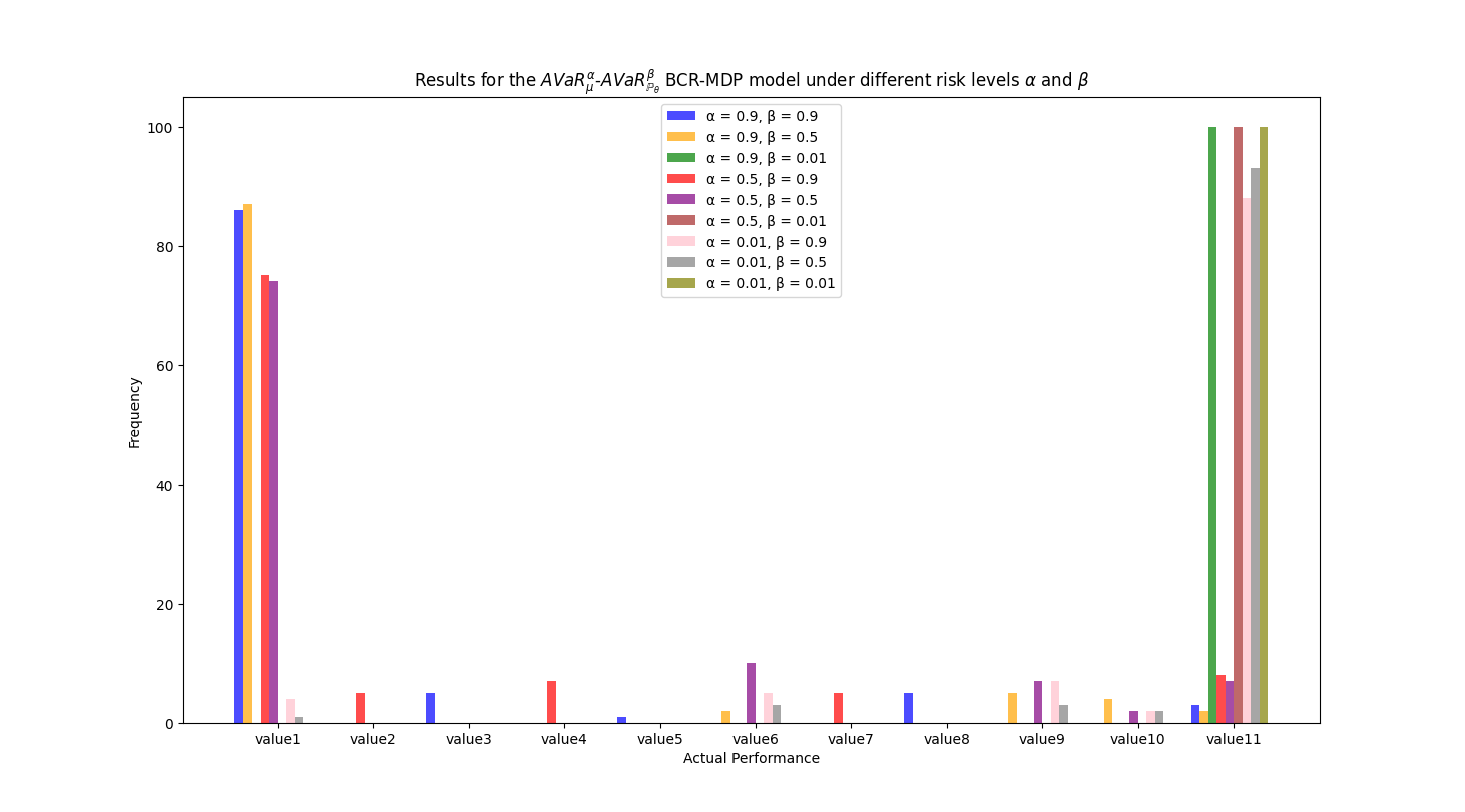
The observations presented in Table 1 and Figure 2 lead to the following conclusions.

•

Compared to the standard SOC/MDP and RA-SOC/MDP, the BCR-SOC/MDP model exhibits better robustness in terms of the mean and variance across different BCR measures (e.g., $\mathbb{E}_{\mu}$ - $\mathbb{E}_{P_{\theta}}$ , $\text{VaR}_{\mu}^{\alpha}$ - $\mathbb{E}_{P_{\theta}}$ and $\text{AVaR}_{\mu}^{\alpha}$ - $\text{AVaR}_{P_{\theta}}^{\beta}$ ). Unlike the methods that depend solely on the point estimate $\hat{\theta}$ , our approach utilizes the distribution $\mu$ to capture the uncertainty in $\theta$ effectively, significantly enhancing the stability of the optimal policy for both small and large sample sizes. Moreover, the DR-SOC/MDP tends to be over conservative, as it always considers the worst-case scenario from the set of all possible market uncertainties, resulting in zero variance in actual performance. In particular, even in situations where the probability of winning at $\theta^{c}$ is high, the DM under DR-SOC/MDP model refrains from betting because of its conservative nature.
•

As the sample size increases, the uncertainty corresponding to the model parameter diminishes. Consequently, the performances of all SOC/MDP models improve consistently, with variance monotonically decreasing. The tendency is underpinned by the convergence of both the posterior distribution $\mu$ and the MLE estimator $\hat{\theta}$ to the true parameter $\theta^{c}$ as the sample size increases. Eventually, every model converges to the SOC/MDP model with respect to the true parameter $\theta^{c}$ in terms of optimal values and optimal policies.
•

In the Bayes-adaptive MDP models (e.g. [38, 55]), we tend to use the augmented pair of the original physical state and the posterior distribution to obtain the optimal value function and policy. Utilizing dynamic programming techniques, we discretize the continuous state, resulting in an exceedingly large augmented state space. As a result of this brute-force approach the computational time for BCR-SOC/MDP model is considerably higher than that of conventional SOC/MDP formulations which involve only a single discrete state physical space $\mathcal{S}$ .
•

In Figure 2, the risk levels $\alpha$ and $\beta$ reflect the bettor’s risk preferences towards the epistemic and aleatoric uncertainties, respectively. With lower values of $\alpha$ and $\beta$ , the DM tends to adopt a more conservative policy, typically choosing not to bet. Consequently, this conservative stance causes the distribution of actual performance to shift toward the right. However, the risk preferences characterized by $\alpha$ and $\beta$ diverge in specific aspects. A lower $\alpha$ indicates a bettor’s increased concern over losses in extreme environment, signifying a preference for avoiding such outcomes. As $\alpha$ decreases, the optimal decisions under BCR-SOC/MDP model closely resemble those of the DR-SOC/MDP approach, resulting in more conservative choices. Conversely, a lower $\beta$ directly signifies a bettor’s aversion to losses, demonstrating prudence and a preference for minimal potential losses. Thus, as $\beta$ decreases, the bettor focuses more on the losses with respect to worst-case $\xi$ irrespective of the environmental parameter $\theta$ , steering the BCR-SOC/MDP model towards the robust SOC/MDP model. This invariably leads to more cautious decisions. Moreover, compared to the risk level $\alpha$ , $\beta$ exerts a stronger influence on the conservativeness of the outcomes. This is because, while the outer conservatism ensures that losses maintain a degree of randomness even in the worst environment, the inner conservatism compels the bettor to directly consider the most adverse scenario.

7.2 Infinite horizon inventory control problem

Having demonstrated the reasonability and efficiency of the proposed BCR-SOC/MDP model compared with typical SOC/MDP models in the literature, in this subsection, we mainly apply the proposed infinite horizon BCR-SOC/MDP model to the inventory control problem with a discount factor $\gamma=0.8$ .

Inventory models have numerous real-world applications, including healthcare systems, electric energy storage systems, and more (see [58, 75] and the references therein). In inventory management, the problem typically involves deciding the order quantity required in each episode to fulfill customer demand while minimizing costs. The goal of the inventory manager is to manage the trade-offs between ordering costs, holding costs, and penalty costs associated with stockouts, while dynamically adjusting orders based on inventory levels and the uncertainty of future demand. A typical risk-averse inventory control problem aims to minimize long-term costs by dynamically adjusting order quantities and updating beliefs about future demand.

To model this dynamic decision-making process using the BCR-SOC/MDP framework, we define the following parameters and assumptions:

(i)

Customer demand $\xi_{t}$ . The random variable $\xi_{t}$ represents the demand for goods at episode $t$ . We assume that the demand $\xi_{t}$ follows a Poisson distribution with an unknown parameter $\theta^{c}$ [61].
(ii)

Inventory level $s_{t}$ . The inventory level at episode $t$ , denoted by $s_{t}$ , represents the quantity of goods available in stock at that episode. Inventory is updated at each episode based on the decision made by the inventory manager (the order quantity) and the actual demand observed during that episode.
(iii)

Belief $\mu_{t}(\theta)$ . The inventory manager’s belief about the demand distribution at episode $t$ , denoted by $\mu_{t}(\theta)$ , represents the manager’s knowledge of the likelihood of various demand amounts. A typical prior $\mu_{1}$ for $\theta$ here is the Gamma prior since the posterior $\mu_{t}$ is also a Gamma distribution (see also [21]).
(iv)

Order quantity $a_{t}$ . The order quantity at episode $t$ , denoted by $a_{t}$ , represents the amount of goods the inventory manager decides to order. This decision $a_{t}$ is determined by the manager’s policy $\pi_{t}(s_{t},\mu_{t})$ , which depends on the current inventory level $s_{t}$ and the inventory manager’s belief $\mu_{t}(\theta)$ about the demand distribution.
(v)

Cost function ${\cal C}$ and state transition function $g$ . The cost ${\cal C}$ at episode $t$ is defined as

$\mathcal{C}(s_{t},a_{t},\xi_{t})=oa_{t}+c(s_{t}+a_{t},\xi_{t}),$

where

$c(y,d):=p\max\{d-y,0\}+h\max\{y-d,0\},$

$o,p$ and $h$ are unit order cost, penalty cost for unfulfilling a unit demand, and unit holding cost for excess inventory, respectively. The inventory level $s_{t+1}$ can then be defined as $s_{t+1}=g(s_{t},a_{t},\xi_{t}):=s_{t}+a_{t}-\xi_{t}$ .

Under the BCR-SOC/MDP framework, the infinite horizon inventory control problem can be formulated as:


$\displaystyle\min_{\pi}\quad$	$\displaystyle\rho_{\mu_{1}}\circ\rho_{P_{\theta_{1}}}\left[oa_{1}+c(s_{1}+a_{1},\xi_{1})+\cdots+\gamma\rho_{\mu_{t}}\circ\rho_{P_{\theta_{t}}}\left[oa_{t}+c(s_{t}+a_{t},\xi_{t})+\cdots\right]\right]$	(7.2a)
s.t.	$\displaystyle s_{t+1}=s_{t}+a_{t}-\xi_{t},\ a_{t}=\pi(s_{t},\mu_{t}),\ a_{t}\geq 0,\ \mu_{t+1}(\theta)=\frac{p\left(\xi_{t}\|\theta\right)\mu_{t}(\theta)}{\int_{\Theta}p\left(\xi_{t}\|\theta\right)\mu_{t}(\theta)d\theta},t=1,2,\cdots.$	(7.2b)

The classical stationary inventory control problem corresponding to the true distribution $P_{\theta^{c}}$ can be described in BCR-SOC/MDP form as follows:

	$\displaystyle\min_{\pi}$	$\displaystyle\rho_{P_{\theta^{c}}}\left[oa_{1}+c(s_{1}+a_{1},\xi_{1})+\cdots+\gamma\rho_{P_{\theta^{c}}}\left[oa_{t}+c(s_{t}+a_{t},\xi_{t})+\cdots\right]\right]$		(7.3)
	s.t.	$\displaystyle s_{t+1}=s_{t}+a_{t}-\xi_{t},\ a_{t}=\pi(s_{t},\delta_{\theta^{c}}),\ a_{t}\geq 0,\ t=1,2,\cdots$		(7.3)

As demonstrated in [63], the optimal policy for problem (7.3) is the base-stock policy $\pi^{*}(s,\delta^{c})=\max\{s^{*}-s,0\}$ , where $s^{*}=H^{-1}(\kappa)$ with $H(\cdot)$ being the cdf of the random demand and $\kappa:=\frac{p-(1-\gamma)o}{p+h}$ . Thus, for $s\leq s^{*}$ , the optimal value of (7.3) is given by:

V^{*}(s,\delta_{\theta^{c}})=-os+os^{*}+(1-\gamma)^{-1}\rho_{P_{\theta^{c}}}[\gamma o\xi+c(s^{*},\xi)].

(7.4)

With this analytical expression, we can compute the true optimal value functions with $\rho_{P_{\theta^{c}}}=\mathbb{E}_{P_{\theta^{c}}}$ and $\rho_{P_{\theta^{c}}}=\text{AVaR}_{P_{\theta^{c}}}^{\beta}$ , respectively, as benchmarks for standard SOC/MDP and risk-averse SOC/MDP to demonstrate the convergence of the BCR-SOC/MDP models corresponding to $\text{VaR}_{\mu}^{\alpha}$ - $\mathbb{E}_{P_{\theta}}$ and $\text{AVaR}_{\mu}^{\alpha}$ - $\text{AVaR}_{P_{\theta}}^{\beta}$ with respect to the value functions.

In this inventory control problem, we set $\Theta=\{6,8,9,10,11,12,14\}$ . The unit cost for ordering is $o=2$ , the unit holding cost is $h=4$ , and the penalty for unmet demand is set at $p=6$ . For the BCR-SOC/MDP model, we set the outer risk parameter $\alpha=0.6$ and the inner risk parameter $\beta=0.4$ . To facilitate comparison with other MDP models, we examine the performance of the model with different true parameter values $\theta^{c}$ . Figure 3 depicts the performance when the learned policy is deployed in various environments with the demand following different Poisson distributions. To illustrate the convergence of optimal value function, we use Algorithm 2 to find the unique optimal value function $V^{*}$ of the Bellman equation corresponding to (7.2a). Then, we generate sample sequences $\bm{\xi}^{t}$ across different episodes $t$ , compute $\mu_{t}$ and obtain the corresponding optimal value $V^{*}(s,\mu_{t})$ . The procedure is replicated 100 times to ensure robustness, and the results are shown in Figures 4 and 5. Specifically, we plot boxplot of the sup-norm of the gap between the estimation $V^{*}(\cdot,\mu_{t})$ and the true optimal value $V^{*}(\cdot,\delta_{\theta^{c}})$ , which is calculated as $\sup_{s\in\mathcal{S}}|V^{*}(s,\mu_{t})-V^{*}(s,\delta_{\theta^{c}})|$ . Moreover, we also use line chart to show the average and standard deviation of the sup-norm of the gap between the estimated value $V^{*}(\cdot,\mu_{t})$ and the true optimal value $V^{*}(\cdot,\delta_{\theta^{c}})$ across different episodes, providing insights into the robustness and variability of the estimation process. We can make the following observations from Figures 3, 4 and 5.

•

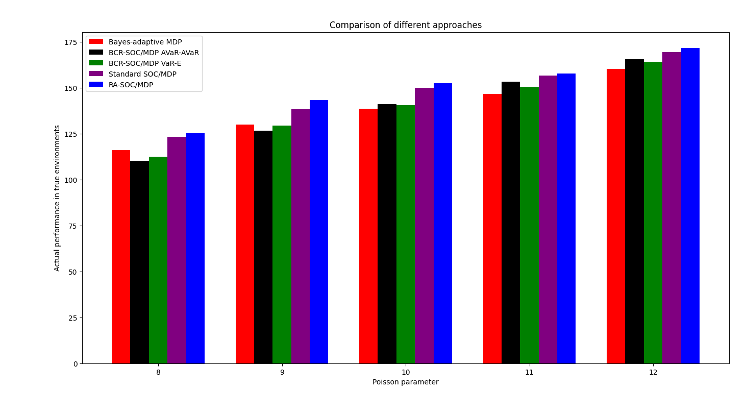
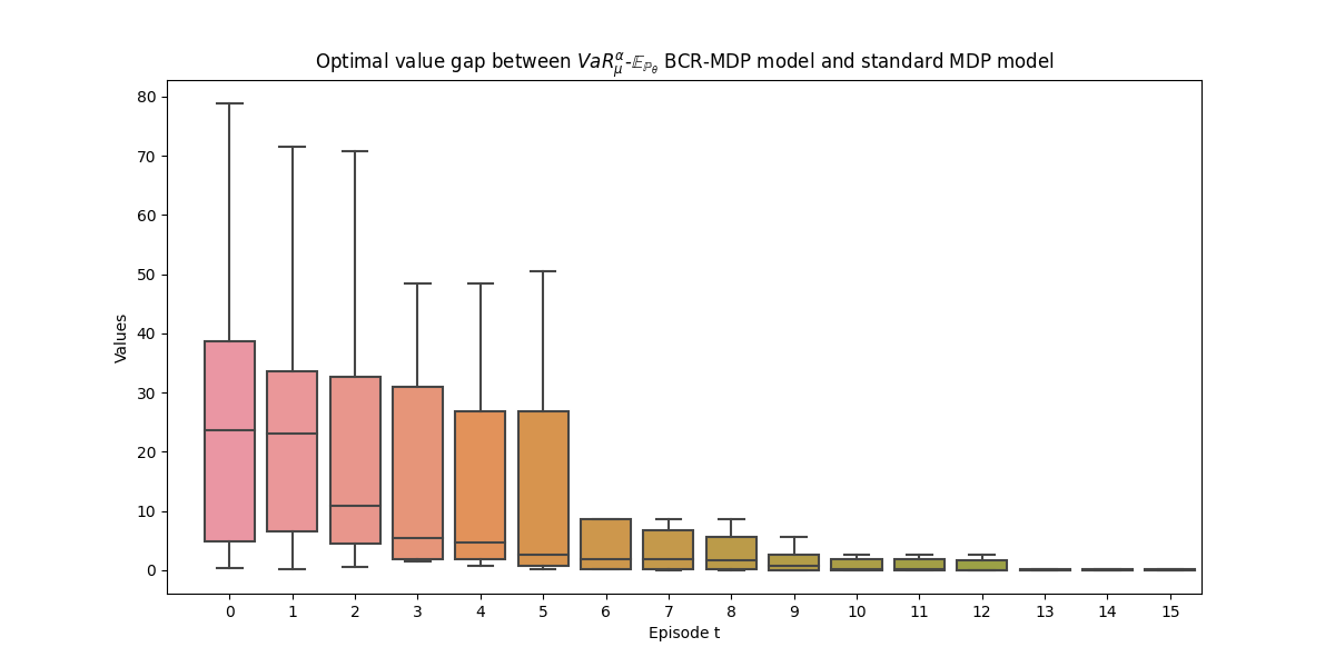
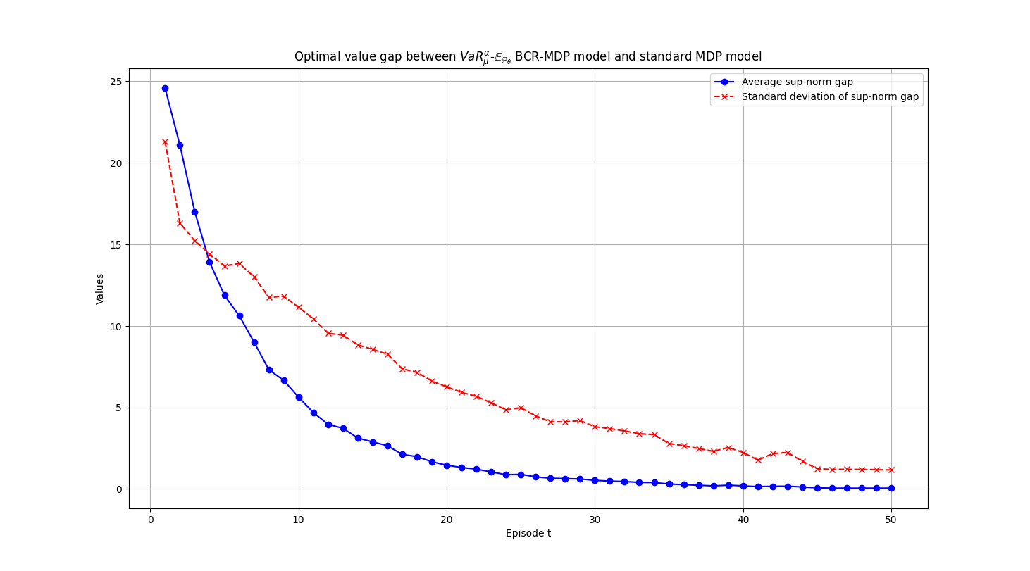
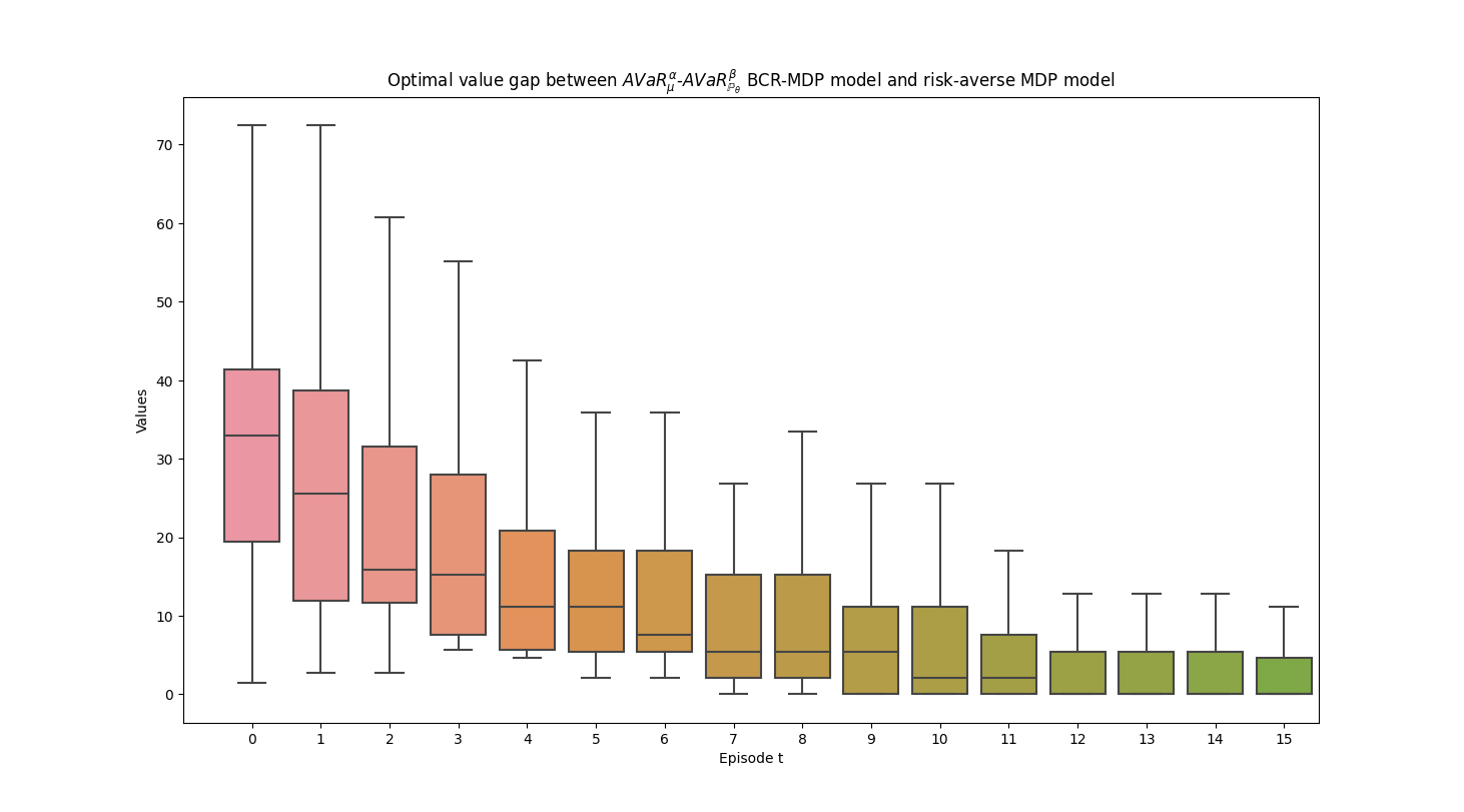
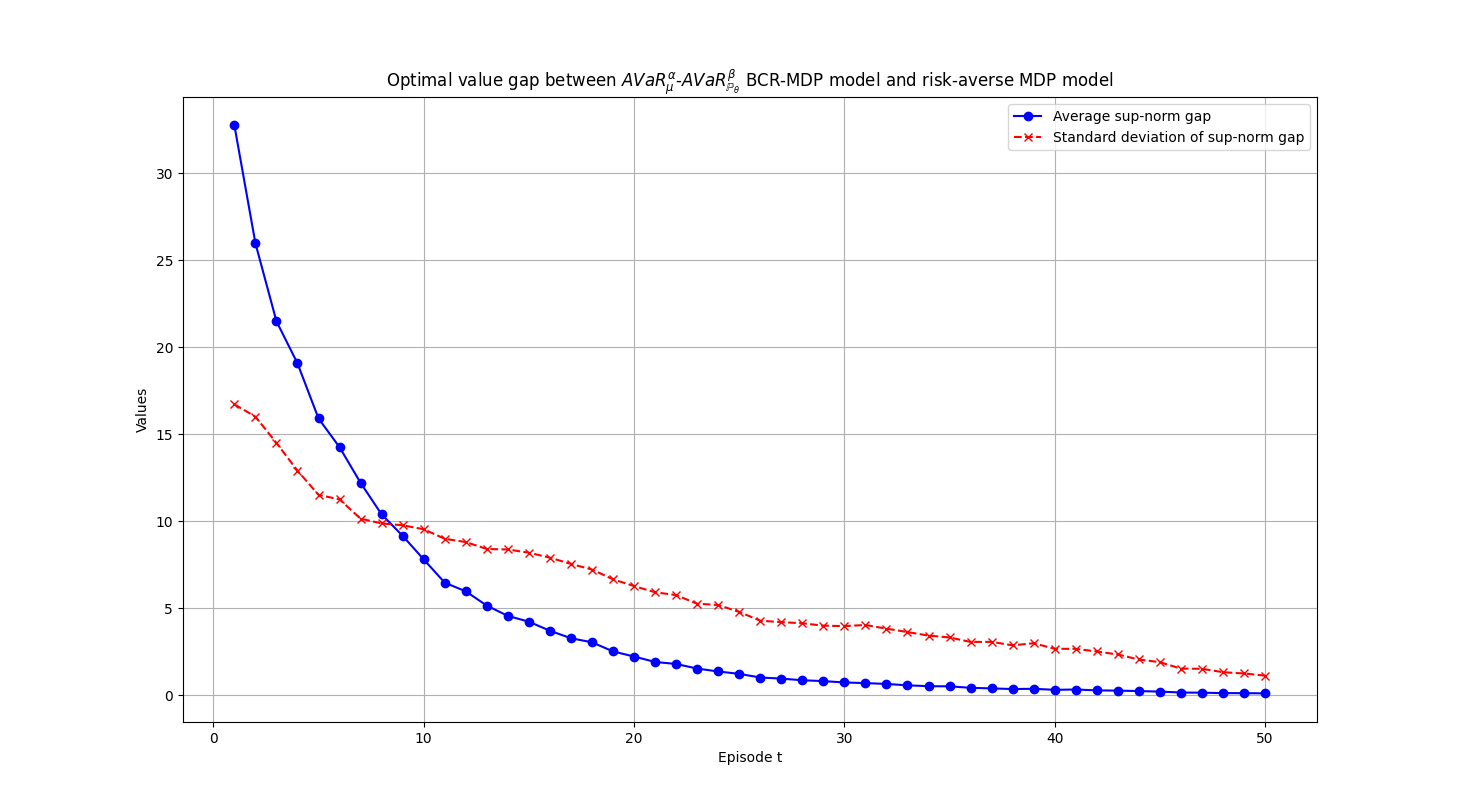
The BCR-SOC/MDP model outperforms the standard SOC/MDP and RA-SOC/MDP models in diverse environments and various BCR measures, such as $\mathbb{E}_{\mu}$ - $\mathbb{E}_{P_{\theta}}$ , $\text{VaR}_{\mu}^{\alpha}$ - $\mathbb{E}_{P_{\theta}}$ and $\text{AVaR}_{\mu}^{\alpha}$ - $\text{AVaR}_{P_{\theta}}^{\beta}$ . Moreover, when compared to the risk-neutral Bayes-adaptive SOC/MDP model, BCR-SOC/MDP models incorporating risk-averse preferences achieve a lower optimal cost value in more adversarial scenarios (e.g., when the Poisson parameter is less than 10), emphasizing their robustness and adaptability to a wide range of challenging environments.
•

The mean, median and the range of the super-norm all decrease to $0$ as $t$ increases, which means that the optimal value functions of all $\text{VaR}_{\mu}^{\alpha}$ - $\mathbb{E}_{P_{\theta}}$ and $\text{AVaR}_{\mu}^{\alpha}$ - $\text{AVaR}_{P_{\theta}}^{\beta}$ BCR-SOC/MDP models display uniform convergence as envisaged by the theoretical results. From the boxplots in Figures 4 and 5, we observe that the convergence rate of the optimal value functions corresponding to the $\text{AVaR}_{\mu}^{\alpha}$ - $\text{AVaR}_{P_{\theta}}^{\beta}$ case is slower than that of the $\text{VaR}_{\mu}^{\alpha}$ - $\mathbb{E}_{P_{\theta}}$ BCR-SOC/MDP model, which is consistent with the conclusion in Theorem 3. Moreover, the line charts in Figures 4 and 5 show that, compared to the $\text{VaR}_{\mu}^{\alpha}$ - $\mathbb{E}_{P_{\theta}}$ BCR-SOC/MDP model, the $\text{AVaR}_{\mu}^{\alpha}$ - $\text{AVaR}_{P_{\theta}}^{\beta}$ BCR-SOC/MDP model exhibits smaller variability in the sup-norm gap, reflecting the more robust characteristics of the latter risk-averse attitude with respect to the value function.
•

As the episode $t$ increases, the elements of the stochastic process $\bm{\xi}^{t}$ increase, and the optimal value function corresponding to state $s$ converges exponentially to the optimal value of the true model as $\mu_{t}$ converges. This manifests the significance and characteristics of Bayes-adaptive MDPs. Specifically, the epistemic uncertainty gradually diminishes as the DM continuously observes/learns about the environment. Consequently, the DM’s understanding of the environment becomes more precise, driving the gap of the optimal values to zero. Likewise, the variability of the gap reduces to zero. By contrast, for a standard SOC/MDP or risk-averse SOC/MDP, once the model is established, the optimal value function remains fixed and does not change over time. Specifically, once an MLE estimator $\hat{\theta}$ is derived for the standard or risk-averse SOC/MDP, the corresponding optimal value function takes a similar form to that in (7.4), with $\theta^{c}$ being replaced by $\hat{\theta}$ . Consequently, for any episode $t$ , the optimal value functions for the estimated SOC/MDP models remain fixed, which explains that these models do not adaptively learn in response to dynamic change of the environment.

8 Concluding remarks

In this paper, we introduce a BCR-SOC/MDP model which subsumes a range of existing SOC/MDP models and relates to preference robust SOC/MDP models. By comparison with [63], the new model exhibits adaptive learning capabilities and ensures robustness against the inherent parameter randomness. In the finite-horizon case, we derive some important properties of the BCR-SOC/MDP model. In the infinite-horizon case, we derive some basic properties and demonstrate the model’s adaptability by showing that as the number of episodes increases, the optimal value functions and optimal policies almost surely converge to those of the true underlying problem. We also propose SAA-type algorithms tailored for solving the BCR-SOC/MDP model under specific composite risk measures and examine the robustness and adaptability of the model through numerical experiments. The theoretical analyses and numerical results show that the monetary risk measure, especially the Value at Risk (VaR), robust spectral risk measure (SRM) and average VaR, also exhibits convergence properties, prompting an examination of how to relax the conditions to encompass a broader range of risk measures.

There are a few aspects that we may take from this work for more in-depth exploration. First, the relationship between the BCR-SOC/MDP and preference-robust SOC/MDP models. We have indicated in Section 3.2 that a relationship between the two models may be established. It might be interesting to investigate the fine details of the relationship between distributionally robustness and preference robustness in the dynamic setting given that both are fundamentally related to DM’s dynamic risk preferences. Moreover, the BCR-SOC/MDP framework may potentially provide a more convenient avenue for solving multistage randomized preference-robust optimization problems [80]. Second, because of the complex structure of the Bayesian composite risk measure and the posterior distributions in the augmented state space, this paper does not explore SDDP-type methods for solving the problem as in [62]. It might be worth discussing SDDP for solving the proposed model at least under some specific cases given the known effectiveness of SDDP approach. Third, in practical application of the BCR-SOC/MDP model, particularly in data-driven problems, samples are often drawn from empirical data which might contain some noise. In that case, it might be relevant to investigate whether the proposed models are stable against perturbations in the uncertainty data in terms of both optimal values and optimal policies. Stability results for conventional SOC/MDP models have been derived by Kern et al. [35], and it would be valuable to explore whether similar stability results can be established for the BCR-SOC/MDP model. Finally, the numerical tests were carried out with two conventional SOC/MDP problems. It will be much more interesting if we can find new applications particularly related to online decision making. We leave all these avenues for future research.

Declarations

•

This project is supported by the National Key R&D Program of China (2022YFA1004000, 2022YFA1004001), National Natural Science Foundation of China (11991023) and CUHK start-up grant.

Acknowledgments

We would like to thank Alex Shapiro and Zhiyao Yang for a number of valuable discussions during preparation of this work.

reference

[1] C. Acerbi, Spectral measures of risk: A coherent representation of subjective risk aversion, Journal of Banking & Finance, 26 (2002), pp. 1505–1518.
[2] M. Ahmadi, U. Rosolia, M. D. Ingham, R. M. Murray, and A. D. Ames, Constrained risk-averse Markov decision processes, in Proceedings of the AAAI Conference on Artificial Intelligence, vol. 35, 2021, pp. 11718–11725.
[3] N. Bäuerle and J. Ott, Markov decision processes with average-value-at-risk criteria, Mathematical Methods of Operations Research, 74 (2011), pp. 361–379.
[4] R. E. Bellman and S. E. Dreyfus, Applied Dynamic Programming, vol. 2050, Princeton University Press, 2015.
[5] D. Bertsekas, Dynamic Programming and Optimal Control: Volume I, Athena scientific, 2012.
[6] J. R. Birge, Y. Feng, N. B. Keskin, and A. Schultz, Dynamic learning and market making in spread betting markets with informed bettors, Operations Research, 69 (2021), pp. 1746–1766.
[7] S. Carpin, Y.-L. Chow, and M. Pavone, Risk aversion in finite Markov decision processes using total cost criteria and average value at risk, in 2016 IEEE International Conference on Robotics and Automation (ICRA), IEEE, 2016, pp. 335–342.
[8] Z. Chen and W. Ma, A Bayesian approach to data-driven multi-stage stochastic optimization, Journal of Global Optimization, 90 (2024), pp. 401–428.
[9] Y. Chow, A. Tamar, S. Mannor, and M. Pavone, Risk-sensitive and robust decision-making: a CVaR optimization approach, Advances in Neural Information Processing Systems, 28 (2015).
[10] M. Claus, Advancing Stability Analysis of Mean-risk Stochastic programs: Bilevel and Two-stage Models, PhD thesis, Dissertation, Duisburg, Essen, Universität Duisburg-Essen, 2016.
[11] R. Dearden, N. Friedman, and D. Andre, Model-based Bayesian exploration, arXiv preprint arXiv:1301.6690, (2013).
[12] E. Delage and D. A. Iancu, Robust multistage decision making, in The operations research revolution, INFORMS, 2015, pp. 20–46.
[13] E. Delage and S. Mannor, Percentile optimization for Markov decision processes with parameter uncertainty, Operations Research, 58 (2010), pp. 203–213.
[14] E. Delage and Y. Ye, Distributionally robust optimization under moment uncertainty with application to data-driven problems, Operations Research, 58 (2010), pp. 595–612.
[15] P. Dommel and A. Pichler, Foundations of Multistage Stochastic Programming, arXiv preprint arXiv:2102.07464, (2021).
[16] M. O. Duff, Optimal Learning: Computational procedures for Bayes-adaptive Markov Decision Processes, University of Massachusetts Amherst, 2002.
[17] J. Dupačová and K. Sladkỳ, Comparison of multistage stochastic programs with recourse and stochastic dynamic programs with discrete time, ZAMM-Journal of Applied Mathematics and Mechanics, 82 (2002), pp. 753–765.
[18] E. A. Feinberg and A. Shwartz, Handbook of Markov Decision Processes: Methods and Applications, vol. 40, Springer Science & Business Media, 2012.
[19] J. A. Filar, D. Krass, and K. W. Ross, Percentile performance criteria for limiting average Markov decision processes, IEEE Transactions on Automatic Control, 40 (1995), pp. 2–10.
[20] R. Gao and A. Kleywegt, Distributionally robust stochastic optimization with Wasserstein distance, Mathematics of Operations Research, 48 (2023), pp. 603–655.
[21] A. Gelman, J. Carlin, H. Stern, D. Dunson, A. Vehtari, and D. Rubin, Bayesian Data Analysis, Third Edition, Chapman & Hall/CRC Texts in Statistical Science, Taylor & Francis, 2013.
[22] V. Guigues, A. Shapiro, and Y. Cheng, Risk-averse stochastic optimal control: an efficiently computable statistical upper bound, Operations Research Letters, 51 (2023), pp. 393–400.
[23] S. Guo and H. Xu, Robust spectral risk optimization when the subjective risk aversion is ambiguous: a moment-type approach, Mathematical Programming, 194 (2022), pp. 305–340.
[24] V. Gupta, Near-optimal bayesian ambiguity sets for distributionally robust optimization, Management Science, 65 (2019), pp. 4242–4260.
[25] H. Gzyl and S. Mayoral, On a relationship between distorted and spectral risk measures., (2008).
[26] J. L. Hau, M. Petrik, and M. Ghavamzadeh, Entropic risk optimization in discounted MDPs, in International Conference on Artificial Intelligence and Statistics, PMLR, 2023, pp. 47–76.
[27] L. Hong and R. Martin, A review of Bayesian asymptotics in general insurance applications, European Actuarial Journal, 7 (2017), pp. 231–255.
[28] R. A. Howard, Dynamic Programming and Markov Processes, John Wiley, 1960.
[29] R. A. Howard and J. E. Matheson, Risk-sensitive Markov decision processes, Management Science, 18 (1972), pp. 356–369.
[30] D. A. Iancu, M. Petrik, and D. Subramanian, Tight approximations of dynamic risk measures, Mathematics of Operations Research, 40 (2015), pp. 655–682.
[31] G. N. Iyengar, Robust dynamic programming, Mathematics of Operations Research, 30 (2005), pp. 257–280.
[32] D. Jalota and Y. Ye, Stochastic online fisher markets: Static pricing limits and adaptive enhancements, Operations Research, (2024).
[33] D. R. Jiang and W. B. Powell, Risk-averse approximate dynamic programming with quantile-based risk measures, Mathematics of Operations Research, 43 (2018), pp. 554–579.
[34] L. V. Kantorovich and S. Rubinshtein, On a space of totally additive functions, Vestnik of the St. Petersburg University: Mathematics, 13 (1958), pp. 52–59.
[35] P. Kern, A. Simroth, and H. Zähle, First-order sensitivity of the optimal value in a Markov decision model with respect to deviations in the transition probability function, Mathematical Methods of Operations Research, 92 (2020), pp. 165–197.
[36] S. Kusuoka, On law invariant coherent risk measures, Advances in mathematical economics, (2001), pp. 83–95.
[37] M. Li, X. Tong, and H. Xu, Randomization of spectral risk measure and distributional robustness, arXiv preprint arXiv:2212.08871, (2022).
[38] Y. Lin, Y. Ren, and E. Zhou, Bayesian risk Markov decision processes, Advances in Neural Information Processing Systems, 35 (2022), pp. 17430–17442.
[39] J. Luedtke and S. Ahmed, A sample approximation approach for optimization with probabilistic constraints, SIAM Journal on Optimization, 19 (2008), pp. 674–699.
[40] W. Ma and Z. Chen, Multi-stage distributionally robust convex stochastic optimization with Bayesian-type ambiguity sets, Mathematical Methods of Operations Research, 100 (2024), pp. 553–600.
[41] S. Mannor, D. Simester, P. Sun, and J. N. Tsitsiklis, Bias and variance in value function estimation, in Proceedings of the twenty-first International Conference on Machine learning, 2004, p. 72.
[42] S. Mannor and J. Tsitsiklis, Mean-variance optimization in Markov decision processes, arXiv preprint arXiv:1104.5601, (2011).
[43] S. Mannor and H. Xu, Data-driven methods for Markov decision problems with parameter uncertainty, in Operations Research & Management Science in the Age of Analytics, INFORMS, 2019, pp. 101–129.
[44] A. Nilim and L. El Ghaoui, Robust control of Markov decision processes with uncertain transition matrices, Operations Research, 53 (2005), pp. 780–798.
[45] I. Osband, D. Russo, and B. Van Roy, (More) efficient reinforcement learning via posterior sampling, Advances in Neural Information Processing Systems, 26 (2013).
[46] T. Osogami and T. Morimura, Time-consistency of optimization problems, in Proceedings of the AAAI Conference on Artificial Intelligence, vol. 26, 2012, pp. 1945–1953.
[47] M. Petrik and D. Subramanian, An approximate solution method for large risk-averse Markov decision processes, arXiv preprint arXiv:1210.4901, (2012).
[48] G. C. Pflug and A. Pichler, Multistage Stochastic Optimization, vol. 1104, Springer, 2014.
[49] A. B. Philpott, V. L. de Matos, and L. Kapelevich, Distributionally robust SDDP, Computational Management Science, 15 (2018), pp. 431–454.
[50] A. Pichler and R. Schlotter, Risk-averse optimal control in continuous time by nesting risk measures, Mathematics of Operations Research, 48 (2023), pp. 1657–1678.
[51] M. L. Puterman, Markov Decision Processes: Discrete Stochastic Dynamic Programming, John Wiley & Sons, 2014.
[52] P. Qian, Z. Wang, and Z. Wen, A composite risk measure framework for decision making under uncertainty, Journal of the Operations Research Society of China, 7 (2019), pp. 43–68.
[53] M. Rigter, B. Lacerda, and N. Hawes, Risk-averse Bayes-adaptive reinforcement learning, Advances in Neural Information Processing Systems, 34 (2021), pp. 1142–1154.
[54] R. T. Rockafellar, S. Uryasev, et al., Optimization of conditional value-at-risk, Journal of risk, 2 (2000), pp. 21–42.
[55] S. Ross, J. Pineau, B. Chaib-draa, and P. Kreitmann, A Bayesian approach for learning and planning in partially observable Markov decision processes., Journal of Machine Learning Research, 12 (2011).
[56] H. Ruan, Z. Chen, and C. P. Ho, Risk-averse MDPs under reward ambiguity, arXiv preprint arXiv:2301.01045, (2023).
[57] A. Ruszczyński, Risk-averse dynamic programming for Markov decision processes, Mathematical Programming, 125 (2010), pp. 235–261.
[58] E. Saha and P. K. Ray, Modelling and analysis of inventory management systems in healthcare: A review and reflections, Computers & Industrial Engineering, 137 (2019), p. 106051.
[59] A. Shapiro, Tutorial on risk neutral, distributionally robust and risk averse multistage stochastic programming, European Journal of Operational Research, 288 (2021), pp. 1–13.
[60] A. Shapiro, Distributionally robust modeling of optimal control, Operations Research Letters, 50 (2022), pp. 561–567.
[61] A. Shapiro, D. Dentcheva, and A. Ruszczynski, Lectures on Stochastic Programming: Modeling and Theory, SIAM, 2021.
[62] A. Shapiro, E. Zhou, and Y. Lin, Bayesian distributionally robust optimization, SIAM Journal on Optimization, 33 (2023), pp. 1279–1304.
[63] A. Shapiro, E. Zhou, Y. Lin, and Y. Wang, Episodic Bayesian optimal control with unknown randomness distributions, arXiv preprint arXiv:2308.08478, (2023).
[64] A. Sharma, J. Harrison, M. Tsao, and M. Pavone, Robust and adaptive planning under model uncertainty, in Proceedings of the international conference on automated planning and scheduling, vol. 29, 2019, pp. 410–418.
[65] M. Sniedovich, A variance-constrained reservoir control problem, Water Resources Research, 16 (1980), pp. 271–274.
[66] H. Strasser, Mathematical Theory of Statistics: Statistical Experiments and Asymptotic Decision Theory, vol. 7, Walter de Gruyter, 1985.
[67] M. Strens, A Bayesian framework for reinforcement learning, in ICML, 2000, pp. 943–950.
[68] A. Tamar, Y. Chow, M. Ghavamzadeh, and S. Mannor, Sequential decision making with coherent risk, IEEE Transactions on Automatic Control, 62 (2016), pp. 3323–3338.
[69] H. Wang, L. He, R. Gao, and F. Calmon, Aleatoric and epistemic discrimination: Fundamental limits of fairness interventions, Advances in Neural Information Processing Systems, 36 (2024).
[70] W. Wang and S. Ahmed, Sample average approximation of expected value constrained stochastic programs, Operations Research Letters, 36 (2008), pp. 515–519.
[71] W. Wang and H. Xu, Robust spectral risk optimization when information on risk spectrum is incomplete, SIAM Journal on Optimization, 30 (2020), pp. 3198–3229.
[72] W. Wang, H. Xu, and T. Ma, Quantitative statistical robustness for tail-dependent law invariant risk measures, Quantitative Finance, 21 (2021), pp. 1669–1685.
[73] Y. Wang and E. Zhou, Bayesian risk-averse Q-Learning with streaming observations, arXiv preprint arXiv:2305.11300, (2023).
[74] S. Weber, Distribution-invariant risk measures, information, and dynamic consistency, Mathematical Finance: An International Journal of Mathematics, Statistics and Financial Economics, 16 (2006), pp. 419–441.
[75] T. Weitzel and C. H. Glock, Energy management for stationary electric energy storage systems: A systematic literature review, European Journal of Operational Research, 264 (2018), pp. 582–606.
[76] W. Wiesemann, D. Kuhn, and B. Rustem, Robust Markov decision processes, Mathematics of Operations Research, 38 (2013), pp. 153–183.
[77] W. Wiesemann, D. Kuhn, and M. Sim, Distributionally robust convex optimization, Operations Research, 62 (2014), pp. 1358–1376.
[78] D. Wozabal, Robustifying convex risk measures for linear portfolios: A nonparametric approach, Operations Research, 62 (2014), pp. 1302–1315.
[79] D. Wu, H. Zhu, and E. Zhou, A Bayesian risk approach to data-driven stochastic optimization: Formulations and asymptotics, SIAM Journal on Optimization, 28 (2018), pp. 1588–1612.
[80] Q. Wu, H. Xu, and H. Zheng, Multistage Robust Average Randomized Spectral Risk Optimization, arXiv preprint arXiv:2409.00892, (2024).
[81] H. Xu, Y. Liu, and H. Sun, Distributionally robust optimization with matrix moment constraints: Lagrange duality and cutting plane methods, Mathematical Programming, 169 (2018), pp. 489–529.
[82] H. Xu and S. Mannor, Distributionally robust Markov decision processes, Advances in Neural Information Processing Systems, 23 (2010).
[83] H. Xu and D. Zhang, Smooth sample average approximation of stationary points in nonsmooth stochastic optimization and applications, Mathematical Programming, 119 (2009), pp. 371–401.
[84] I. Yang, Wasserstein distributionally robust stochastic control: A data-driven approach, IEEE Transactions on Automatic Control, 66 (2020), pp. 3863–3870.
[85] S. Zhang, H. Xu, and H. Sun, Statistical Robustness of Kernel Learning Estimator with Respect to Data Perturbation, arXiv preprint arXiv:2406.10555, (2024).

9 Appendix

Definition 2 (Fortet-Mourier metric).

Let

\displaystyle\mathcal{F}_{p}(Z):=\left\{h:Z\rightarrow\mathbb{R}:|h({\bm{z}}^{\prime})-h({{\bm{z}}^{\prime\prime}})|\leq L_{p}({\bm{z}}^{\prime},{{\bm{z}}^{\prime\prime}})\|{\bm{z}}^{\prime}-{{\bm{z}}^{\prime\prime}}\|,\forall{\bm{z}}^{\prime},{{\bm{z}}^{\prime\prime}}\in Z\right\}

(9.1)

be the set of locally Lipschitz continuous functions of growth order $p$ , where $\|\cdot\|$ denotes some norm on $Z$ , $L_{p}({\bm{z}}^{\prime},{{\bm{z}}^{\prime\prime}}):=\max\{1,\|{\bm{z}}^{\prime}\|,\|{{\bm{z}}^{\prime\prime}}\|\}^{p-1}$ for all ${\bm{z}}^{\prime},{{\bm{z}}^{\prime\prime}}\in Z$ , and $p\geq 1$ describes the growth of the local Lipschitz constants. The $p$ -th order Fortet-Mourier metric over $\mathscr{P}(Z)$ is defined by

\displaystyle\mathsf{d\kern-0.70007ptl}_{\rm FM}(P^{\prime},P^{\prime\prime}):=\sup_{h\in\mathcal{F}_{p}(Z)}\left|\int_{Z}h({\bm{z}})P^{\prime}(d{\bm{z}})-\int_{Z}h({\bm{z}})P^{\prime\prime}(d{\bm{z}})\right|,\forall P^{\prime},P^{\prime\prime}\in\mathscr{P}(Z).

(9.2)

In the case when $p=1$ , it reduces to Kantorovich metric, in which case we denote the distance by $\mathsf{d\kern-0.70007ptl}_{K}$ .

Definition 3 (Wasserstein distance/ metric).

For probability measures $P$ and $\tilde{P}$ , the Wasserstein distance/ metric of order $r\geq 1$ is

\mathsf{d\kern-0.70007ptl}_{W}^{r}(P,\tilde{P})=\left(\inf_{\pi}\iint d\left(\xi,\tilde{\xi}\right)^{r}\pi(\mathrm{d}\xi,\mathrm{d}\tilde{\xi})\right)^{\frac{1}{r}},

(9.3)

where $\pi$ is among all probability measure with marginals $P$ and $\tilde{P}$ , i.e.,

	$\displaystyle P(A)$	$\displaystyle=\pi(A\times\Xi),\quad A\in\mathscr{B}(\Xi)\ \text{ and}$
	$\displaystyle\tilde{P}(B)$	$\displaystyle=\pi(\Xi\times B),\quad B\in\mathscr{B}(\Xi).$		(9.4)

One of the main results concerning the Wasserstein distance is the Kantorovich–Rubinstein Theorem ([34]), which establishes a relationship between the Kantorovich metric of two probability measures and the Wasserstein distance when $r=1$ , i.e.,

\mathsf{d\kern-0.70007ptl}_{W}^{1}(P,\tilde{P})=\mathsf{d\kern-0.70007ptl}_{K}(P,\tilde{P}).

(9.5)

		$\displaystyle\left\|\rho_{\mu_{t}}\circ\rho_{P_{\theta_{t}}}\left[\mathcal{C}_{t}\left(s_{t}^{1},{a}_{t},\xi_{t}\right)+\gamma V^{}_{t+1}\left(g_{t}(s_{t}^{1},a_{t},\xi_{t}),\mu^{\prime}\right)\right]-\rho_{\mu_{t}}\circ\rho_{P_{\theta_{t}}}\left[\mathcal{C}_{t}\left(s_{t}^{2},{a}_{t},\xi_{t}\right)+\gamma V^{}_{t+1}\left(g_{t}(s_{t}^{2},a_{t},\xi_{t}),\mu^{\prime}\right)\right]\right\|$
	$\displaystyle\leq$	$\displaystyle\rho_{\mu_{t}}\circ\rho_{P_{\theta_{t}}}\left\|\mathcal{C}_{t}\left(s_{t}^{1},{a}_{t},\xi_{t}\right)+\gamma V^{}_{t+1}\left(g_{t}(s_{t}^{1},a_{t},\xi_{t}),\mu^{\prime}\right)-\mathcal{C}_{t}\left(s^{2}_{t},{a}_{t},\xi_{t}\right)-\gamma V^{}_{t+1}\left(g_{t}(s_{t}^{2},a_{t},\xi_{t}),\mu^{\prime}\right)\right\|$
	$\displaystyle\leq$	$\displaystyle\rho_{\mu_{t}}\circ\rho_{P_{\theta_{t}}}\left(L_{\mathcal{C}}\left\\|s_{t}^{1}-s_{t}^{2}\right\\|+\gamma L_{V_{t+1}}\left\\|g_{t}(s_{t}^{1},a_{t},\xi_{t})-g_{t}(s_{t}^{2},a_{t},\xi_{t})\right\\|\right)$
	$\displaystyle\leq$	$\displaystyle(L_{\mathcal{C}}+\gamma L_{V_{t+1}}L_{g})\left\\|s_{t}^{1}-s_{t}^{2}\right\\|.$

		$\displaystyle V_{t}^{}(s_{t}^{1},\mu_{t})-V_{t}^{}(s_{t}^{2},\mu_{t})$
	$\displaystyle\leq$	$\displaystyle\sup_{a_{t}\in\mathcal{A}}\left\|\rho_{\mu_{t}}\circ\rho_{P_{\theta_{t}}}[\mathcal{C}_{t}\left(s_{t}^{1},a_{t},\xi_{t}\right)+\gamma V^{}_{t+1}\left(g_{t}(s_{t}^{1},{a}_{t},\xi_{t}),\mu^{\prime}\right)]-\rho_{\mu_{t}}\circ\rho_{P_{\theta_{t}}}[\mathcal{C}_{t}\left(s^{2}_{t},{a}_{t},\xi_{t}\right)-\gamma V^{}_{t+1}\left(g_{t}(s_{t}^{2},a_{t},\xi_{t}),\mu^{\prime}\right)]\right\|$
	$\displaystyle\leq$	$\displaystyle(L_{\mathcal{C}}+\gamma L_{V_{t+1}}L_{g})\left\\|s_{t}^{1}-s_{t}^{2}\right\\|.$

		$\displaystyle\|\mathcal{C}_{t}\left(s_{t},a_{t}^{1},\xi_{t}\right)+\gamma V^{}_{t+1}\left(g_{t}(s_{t},a_{t}^{1},\xi_{t}),\mu^{\prime}\right)-\mathcal{C}_{t}\left(s_{t},a_{t}^{2},\xi_{t}\right)+\gamma V^{}_{t+1}\left(g_{t}(s_{t},a_{t}^{2},\xi_{t}),\mu^{\prime}\right)\|$
	$\displaystyle\leq$	$\displaystyle L_{\mathcal{C}}\left\\|a_{t}^{1}-a_{t}^{2}\right\\|+\gamma L_{V_{t+1}}\|\|g_{t}(s_{t},a_{t}^{1},\xi_{t})-g_{t}(s_{t},a_{t}^{2},\xi_{t})\|\|$
	$\displaystyle\leq$	$\displaystyle(L_{\mathcal{C}}+\gamma L_{V_{t+1}}L_{g})\left\\|a_{t}^{1}-a_{t}^{2}\right\\|$

	$\displaystyle\|\psi_{s,a}(\theta)\|=$	$\displaystyle\left\|\rho_{P_{\theta}}\left[\mathcal{C}(s,a,\xi)+\gamma V^{}\left(s^{\prime},\mu_{t+1}\right)\right]-\rho_{P_{\theta^{c}}}\left[\mathcal{C}(s,a,\xi)+\gamma V^{}\left(s^{\prime},\mu_{t+1}\right)\right]\right\|$
	$\displaystyle=$	$\displaystyle\left\|\inf_{\phi\in\Phi}\mathbb{E}_{P_{\theta}}[\Psi(\mathcal{C}(s,a,\xi)+\gamma V^{}\left(s^{\prime},\mu_{t+1}\right),\phi)]-\inf_{\phi\in\Phi}\mathbb{E}_{P_{\theta^{c}}}[\Psi(\mathcal{C}(s,a,\xi)+\gamma V^{}\left(s^{\prime},\mu_{t+1}\right),\phi)]\right\|$
	$\displaystyle\leq$	$\displaystyle\sup_{\phi\in\Phi}\left\|\mathbb{E}_{P_{\theta}}[\Psi(\mathcal{C}(s,a,\xi)+\gamma V^{}\left(s^{\prime},\mu_{t+1}\right),\phi)]-\mathbb{E}_{P_{\theta^{c}}}[\Psi(\mathcal{C}(s,a,\xi)+\gamma V^{}\left(s^{\prime},\mu_{t+1}\right),\phi)]\right\|$
	$\displaystyle\leq$	$\displaystyle K\int\|p(\xi\|\theta)-p(\xi\|\theta^{c})\|d\xi\leq 2KL_{p}\|\theta-\theta^{c}\|,$

	$\displaystyle\left\\|V^{\pi^{\varepsilon,*}}-V_{k+1}\right\\|_{\infty}=$	$\displaystyle\left\\|\mathcal{T}^{\pi^{\varepsilon,}}V^{\pi^{\varepsilon,}}-V_{k+1}\right\\|_{\infty}$
	$\displaystyle\leq$	$\displaystyle\left\\|\mathcal{T}^{\pi^{\varepsilon,}}V^{\pi^{\varepsilon,}}-\mathcal{T}V_{k+1}\right\\|_{\infty}+\left\\|\mathcal{T}V_{k+1}-V_{k+1}\right\\|_{\infty}$
	$\displaystyle=$	$\displaystyle\left\\|\mathcal{T}^{\pi^{\varepsilon,}}V^{\pi^{\varepsilon,}}-\mathcal{T}^{\pi^{\varepsilon,*}}V_{k+1}\right\\|_{\infty}+\left\\|\mathcal{T}V_{k+1}-V_{k+1}\right\\|_{\infty}$
	$\displaystyle\leq$	$\displaystyle\gamma\left\\|V^{\pi^{\varepsilon,*}}-V_{k+1}\right\\|_{\infty}+\gamma\left\\|V_{k+1}-V_{k}\right\\|_{\infty}.$