A Bayesian Framework for Multivariate Differential Analysis Accounting for Missing Data
1 MRC Biostatistics Unit, University of Cambridge, United Kingdom.
2 Université Paris-Saclay, INRAE, AgroParisTech, GABI, France.
3 Université Paris-Saclay, AgroParisTech, INRAE, UMR MIA Paris-Saclay, France.
∗ Corresponding author: marie.chion@protonmail.com
Abstract
Current statistical methods in differential proteomics analysis generally leave aside several challenges, such as missing values, correlations between peptides’ intensities and uncertainty quantification. Moreover, they provide point estimates, such as the mean intensity for a given peptide or protein in a given condition. Whether an analyte should be considered as differential is based on comparisons of p-values with a significance threshold, usually 5%. In the state-of-the-art limma approach, a hierarchical model is used to deduce the posterior distribution of the variance estimator for each analyte. The expectation of this distribution is then used as a moderated estimate of variance and is injected directly into the expression of the t-statistic. However, instead of merely relying on the moderated estimates, we could provide more informative and intuitive results by leveraging a fully Bayesian approach, hence allowing uncertainty quantification. The present work introduces this idea by leveraging standard results from Bayesian inference with conjugate priors in hierarchical models to derive a methodology tailored to handle multiple imputation contexts. Furthermore, a more general problem is tackled through multivariate differential analysis to account for possible inter-peptide correlations. By defining a hierarchical model with prior distributions on both mean and variance parameters, we achieve a global quantification of the uncertainty for differential analysis. Inference is performed by computing the posterior distribution for the difference in mean peptide intensities between two experimental conditions. In contrast to more flexible models that can be achieved with hierarchical structures, our choice of conjugate priors maintains analytical expressions for direct sampling from posterior distributions. Extensive simulation studies have evaluated the performance of this approach, which has been applied to several real-world controlled data sets. We demonstrated its ability to provide more accurate and intuitive results than standard hypothesis testing methods for handling differential analysis in proteomics at a comparable computational cost.
1 Introduction
Context.
Differential proteomics analysis aims to compare peptide and/or protein expression levels across several biological conditions. The amount of data provided by label-free mass spectrometry-based quantitative proteomics experiments requires reliable statistical modelling tools to assess which proteins are differentially abundant. In summary, Table 1 presents the main state-of-the-art routines for differential proteomics analysis. They are based on well-known statistical methods, although facing several challenges. First, while quantitative proteomics data usually contain missing values, they rely on complete datasets. In label-free quantitative proteomics, missing value proportion ranges between 10% and 50% according to Lazar et al. (2016). Imputation remedies this problem by replacing a missing value with a user-defined one. In particular, multiple imputation (Little and Rubin, 2019) consists of generating several imputed datasets, which are combined to obtain an estimator of the parameter of interest (often peptide or protein’s mean intensity under a given condition) and an estimator of its variability. Recent work in Chion et al. (2022) includes the uncertainty induced by the multiple imputation process in the moderated -testing framework, previously described in Smyth (2004). This approach relies on a hierarchical model to deduce the posterior distribution of the variance estimator for each analyte. The expectation of this distribution is used as a moderated estimation of variance and is substituted into the expression of the -statistic.
Despite such theoretical advances, traditional tools such as -tests or more recent variations like those presented in Table 1 sometimes appear limited or old-fashioned. Inference based on Null Hypothesis Significance Testing (NHST) and p-values has been widely questioned over the past decades. Many authors demonstrated that NHST often leads to underestimated rates of false discoveries, publication bias, and contributes as a major factor to the reproducibility crisis in experimental science (Ioannidis, 2005; Colquhoun, 2014; Wasserstein et al., 2019). Additionally, NHST does not provide insights about effect sizes or uncertainty quantification in contrast with frameworks such as Bayesian statistics, which constitute a valuable alternative in most cases Kruschke and Liddell (2018)). The topic of missing data has been under investigation in the Bayesian community for a long time, particularly in simple cases involving conjugate priors (Dominici et al., 2000). Recently, some authors provided convenient approaches and associated implementations (Kruschke, 2013) to handle differential analysis problems with Bayesian inference. For instance, the R package BEST (standing for Bayesian Estimation Supersedes T-test) has widely contributed to the diffusion of those practices in experimental fields. Subsequently, in the proteomics field, O’Brien et al. (2018) suggested a Bayesian selection model to mitigate the problem of missing values, while The and Käll (2019) implemented in Triqler a probabilistic model accounting for different sources of variability from identification and quantification to differential analysis. More generally, Crook et al. (2022) reviewed the contributions of Bayesian statistics to proteomics data analysis.
Finally, to the best of our knowledge, no framework has been proposed so far for conducting multivariate differential analysis in quantitative proteomics. Although traditional differential analysis routines usually perform on thousands of peptides simultaneously, their computations are based on an underlying hypothesis of independence across analytes. However, the existence of correlations, for instance, between peptides of the same protein, seems like a reasonable assumption. Modelling and accounting for such structures explicitly could enhance the ability to discover and quantify meaningful differences between groups or conditions. In response to the aforementioned methodological issues, we propose a novel framework for differential analysis accounting for missing data, uncertainty quantification, and correlations, with an emphasis on the particular context of quantitative proteomics.
| Method | Software | |||
|---|---|---|---|---|
| t-tests |
|
|||
| ANOVA |
|
|||
| Moderated t-test (limma) |
|
|||
| Linear model |
|
Contribution.
By taking advantage of standard results of Bayesian inference with conjugate priors in hierarchical models, we derive a fully Bayesian framework for differential analysis tailored to handle missing data and multiple imputations, often arising in proteomics. Furthermore, we propose to take one step further and tackle a more general problem of multivariate differential analysis to account for possible correlations between analytes. We propose a hierarchical model with prior distributions on both mean and variance parameters to provide well-calibrated quantification of the uncertainty for subsequent differential analysis. The inference is performed by computing the posterior distribution for the difference in mean peptide intensity between two experimental conditions. In contrast to more flexible models with complex hierarchical structures, our choice of conjugate priors maintains analytical expressions for directly sampling from posterior distributions without requiring time-consuming Monte Carlo Markov Chain (MCMC) methods. This results in a fast inference scheme comparable to classical NHST procedures while providing more interpretable results expressed as probabilistic statements.
Outline.
The paper is organised as follows: Section 2.1 presents well-known results about Bayesian inference for Gaussian-inverse-gamma conjugated priors. Following analogous results for the multivariate case, Section 2.2 introduces a general Bayesian framework for evaluating mean differences in differential proteomics context. Section 2.3 provides insights on the particular case where the considered analytes are uncorrelated. The proofs of these methodological developments can be found in Section 5. Section 3 evaluates our framework, called ProteoBayes, through an extensive simulation study and comparisons with existing approaches. We further illustrated hands-on examples on real proteomics datasets and highlighted the benefits of such a multivariate Bayesian framework for practitioners.
2 Modelling
2.1 Bayesian inference for Normal-Inverse-Gamma conjugated priors
Before deriving our complete workflow, let us recall some classical Bayesian inference results that will further serve our aim. We assume a generative model such that a measurement (typically, the peptide intensity) comes from the following expression:
-
•
is the prior distribution over the mean,
-
•
is the error term,
-
•
is the prior distribution over the variance,
with an arbitrary set of prior hyper-parameters. In Figure 1, we provide an illustration summarising these hypotheses.
From the previous assumptions, we can deduce the likelihood of the model for a sample of observations :
Let us recall that the proposed prior, known as Gaussian-inverse-gamma, is conjugated with the Gaussian likelihood with unknown mean and variance . The probability density function (PDF) of such a prior distribution can be written as follows:
In this particular case, it is a well-known result that the inference is tractable, and the posterior distribution remains a Gaussian-inverse-gamma (Murphy, 2007). We provided an extended proof of this result in Section 5.1. Therefore, the joint posterior distribution can be expressed as:
| (1) |
with:
-
•
,
-
•
,
-
•
,
-
•
.
Although these updating expressions for hyper-parameters already provide a valuable result, we shall see in the sequel that we are more interested in the marginal distribution over the mean parameter for comparison purposes. Computing this marginal from the joint posterior in Equation 1 remains tractable as well by integrating over :
with:
-
•
,
-
•
.
The marginal posterior distribution over can thus be expressed as a non-standardised Student’s -distribution that we express below in terms of the initial hyper-parameters:
| (2) |
We shall see in the next section how to leverage this approach to introduce a novel comparison-of-means methodology based on such analytical posterior computations.
2.2 General Bayesian framework for evaluating mean differences
Recalling our differential proteomics context that assesses the differences in mean intensity values for peptides or proteins quantified in samples divided into groups (also called conditions). As before, Figure 2 illustrates the hierarchical generative structure assumed for each group .
Maintaining the notation analogous to previous ones, the generative model for , can be written as:
where:
-
•
is the prior mean intensities vector of the -th group,
-
•
is the error term of the -th group,
-
•
is the prior variance-covariance matrix of the -th group,
with a set of hyper-parameters that needs to be chosen as modelling hypotheses and represents the inverse-Wishart distribution, used as the conjugate prior for an unknown covariance matrix of a multivariate Gaussian distribution (Bishop, 2006).
Traditionally, in Bayesian inference, those quantities must be carefully chosen for the estimation to be as accurate as possible, particularly with low sample sizes. Incorporating expert or prior knowledge in the model would also come from the adequate setting of these hyper-parameters. We discuss in more detail the choice and influence of those prior hyper-parameters in Section 3.3. However, this article’s final purpose is not to estimate but to compare the mean of different groups (i.e., differential analysis). Interestingly, providing a perfect estimation of the posterior distributions over does not appear as the main concern here, as the posterior difference of means (i.e. represents the actual quantity of interest. Although providing meaningful prior hyper-parameters leads to adequate uncertainty quantification, we shall take those quantities equal between all groups to ensure an unbiased comparison.
The present framework aspires to estimate a posterior distribution for each mean parameter vector , starting from the same prior assumptions in each group. The comparison between the means of all groups would then only rely on the ability to sample directly from these distributions and compute empirical posteriors for the means’ difference. As a bonus, this framework remains compatible with multiple imputations strategies previously introduced to handle missing data that frequently arise in applicative contexts (Chion et al., 2022). From the previous hypotheses, we can deduce the likelihood of the model for an i.i.d. sample :
However, as previously pointed out, such datasets often contain missing data, and we shall introduce here consistent notation. Assume to be the set of all observed data, we additionally define:
-
•
, the set of elements that are observed in the -th group,
-
•
, the set of elements that are missing the -th group.
Moreover, as we remain in the context of multiple imputation, we define as the set of draws of an imputation process applied on missing data in the -th group. In such context, a closed-form approximation for the multiple-imputed posterior distribution of can be derived for each group as stated in Proposition 1.
Proposition 1.
For all , the posterior distribution of can be approximated by a mixture of multiple-imputed multivariate -distributions, such as:
with:
-
•
,
-
•
,
-
•
,
where we introduced the shorthand to represent the -th imputed vector of observed data, and the corresponding average vector .
The proof of Proposition 1 can be found in Section 5.2. This analytical formulation is particularly convenient for approximating, using multiple-imputed datasets, the posterior distribution of the mean vector for each group. Although such a linear combination of multivariate -distributions is not a known specific distribution in itself, it is now straightforward to generate realisations of posterior samples by simply drawing from the multivariate -distributions, each being specific to an imputed dataset, and then compute the mean of the vectors. Therefore, the empirical distribution resulting from a high number of samples generated by this procedure would be easy to visualise and manage for comparison purposes. Generating the empirical distribution of the mean’s difference between two groups and comes directly by computing the difference between each couple of samples drawn from both posterior distributions and . In Bayesian statistics, relying on empirical distributions drawn from the posterior is common practice in the context of Markov chain Monte Carlo (MCMC) algorithms but often comes at a high computational cost. In our framework, we managed to maintain analytical distributions from model hypotheses to benefit from probabilistic inference with adequate uncertainty quantification while remaining tractable and not relying on MCMC procedures. Therefore, the computational cost of the method roughly remains as low as frequentist counterparts, as inference merely requires updating hyper-parameter values and drawing from corresponding -distributions. Empirical evidence of this claim is provided in the further simulation study and summarised in Table 2.
As usual, when it comes to comparing the mean between two groups, we still need to assess if the posterior distribution of the difference appears, in a sense, to be sufficiently away from zero. This practical inference choice is not specific to our context and remains highly dependent on the context of the study. Moreover, as the present model is multi-dimensional, we may also question the metric used to compute the difference between vectors. In a sense, our posterior distribution of means’ differences offers an elegant solution to the traditional problem of multiple testing often encountered in applied science and calls for tailored definitions of what could be called a meaningful result (significant does not appear as an appropriate term anymore in this more general context). For example, displaying the distribution of the squared difference would penalise large differences in elements of the mean vector. In contrast, the absolute difference would give a more balanced conception of the average divergence from one group to the other. Clearly, as any marginal of a multivariate -distribution remains a (multivariate) -distribution, comparing specific elements of the mean vectors merely by restraining to the appropriate dimension is also straightforward. In particular, comparing two groups in the univariate case would be a particular case of Proposition 1 with . Recalling our proteomics context, we could still compare the mean intensity of peptides between groups, one peptide at a time, or choose to compare all peptides at once, accounting for possible correlations between peptides in each group. However, an appropriate manner of accounting for those correlations could be to group peptides according to their reference protein. Let us provide in Algorithm 1 a summary of the overall procedure for comparing mean vectors of two different experimental conditions (i.e. Bayesian multivariate differential analysis).
2.3 The uncorrelated case: no more multiple testing nor imputation
Let us notice that modelling covariances between all variables as in Proposition 1 often constitutes a challenge, which is computationally expensive in high dimensions and not always adapted. However, we detailed in Section 2.1 results that, although classical in Bayesian statistics, remain too rarely exploited in applied science. In particular, we can leverage these results to adapt Algorithm 1 to the univariate case for handling the same problem as in Chion et al. (2022) with a probabilistic flavour. In the classical setting of the absence of correlations between peptides (i.e. being diagonal), the problem reduces to the analysis of independent inference problems (as is supposed Gaussian) and the posterior distributions can be derived in closed-form, as we recalled in Equation 1. Moreover, let us highlight a pleasant property coming from relaxing this assumption that (multiple-)imputation is no longer needed in this context. Using the same notation as before and the uncorrelated assumption (and thus the induced independence between analytes for ), we can write:
| (3) | ||||
| (4) | ||||
| (5) | ||||
| (6) | ||||
| (7) | ||||
| (8) |
with:
-
•
,
-
•
.
It can be noticed that factorises naturally over , and thus only depends upon the data that have actually been observed for each peptide. We observe that integrating over missing data is straightforward in this framework, and neither Rubin’s approximation nor imputation (whether multiple or not) appears necessary. The observed data already bear all relevant information as if each unobserved value could merely be ignored without effect on the posterior distribution.
Let us emphasise that this property of factorisation and tractable integration over missing data comes directly from the covariance structure as a diagonal matrix and thus only constitutes a particular case of the previous model, though convenient. It should also be noted that this result only stands for values that are called Missing At Random (MAR). The more complicated Missing Not At Random (MNAR) scenario remains to be studied and is outside the scope of the present paper. However, in differential proteomics, the most common practice is to analyse each peptide as an independent problem. Under this assumption, the Bayesian framework tackles the missing data issue in a natural and somewhat simpler way.
Moreover, classical inference tools based on hypothesis testing perform numerous successive tests for all peptides. Such an approach often leads to the pitfall of multiple testing that must be carefully dealt with. Interestingly, we notice that the above model also avoids multiple testing (as it does not rely on hypothesis testing and the definition of some threshold) while maintaining the convenient interpretations of Bayesian probabilistic inference. To conclude, whereas the analytical derivation of posterior distributions with Gaussian-inverse-gamma constitutes a well-known result, our proposition to define such probabilistic mean’s comparison procedure provides, under the standard uncorrelated-peptides assumption, an elegant and handy alternative to classical techniques that alleviates both imputation and multiple testing issues. Let us provide in Algorithm 2 the pseudo-code summarising the univariate inference procedure and highlight differences with the fully-correlated case:
3 Experiments
In this section, we illustrate and provide empirical evidence that our framework recovers consistent results on simulated datasets, and confirm this behaviour on real controlled datasets.
3.1 Simulated datasets
To generate simulated datasets to evaluate the performance of our method, called ProteoBayes, we used the generative model presented in Figure 1. A Gaussian distribution is taken as a baseline reference. To compute mean differences between groups, we generated samples from various distributions where and will vary depending on the context. Unless otherwise stated, each experiment is repeated 1000 times, and the results are averaged using computed mean values and standard deviations of the metrics. In each group, we observe 5 distinct samples.
3.2 Real datasets
Full datasets
Further, we evaluate our methodology on real datasets using four well-calibrated proteomics experiments, cited in previous methodological works (Chion et al., 2022; Etourneau et al., 2023). These experiments use a ”spike-in” design, which helps us determine which peptides are expected to show differences in expression. Hence, they provide a diverse and robust framework for benchmarking our method under various experimental conditions.
-
•
The Muller2016 dataset refers to the experiment from Muller et al. (2016), where a mixture of UPS1 proteins has been spiked in increasing amounts (0.5, 1, 2.5, 5, 10, and 25 fmol) in a constant background of Saccharomyces cerevisiae lysate (yeast), with each condition analysed in triplicate using a data-dependent acquisition method. This dataset is available on the ProteomeXchange website using the PXD003841 identifier.
-
•
The Bouyssie2020 dataset from Bouyssié et al. (2020) is similar to Muller_2016 but expands the range of UPS1 spike-in concentrations to include ten levels (0.01, 0.05, 0.1, 0.25, 0.5, 1, 5, 10, 25, and 50 fmol), with each condition analysed in quadruplicate. The dataset is available on ProteomeXchange using the PXD009815 identifier.
-
•
The Huang2020 dataset from Huang et al. (2020) features UPS2 proteins spiked at five concentrations (0.75, 0.83, 1.07, 2.04, and 7.54 amol) into of mouse cerebellum lysate, analysed in pentaplicate using a data-independent acquisition (DIA) method. The dataset is available on the ProteomeXchange repository using the PXD016647 identifier.
-
•
The Chion2022 dataset refers to the ARATH dataset from Chion et al. (2022), where a mixture of UPS1 proteins spiked at seven increasing concentrations (0.05, 0.25, 0.5, 1.25, 2.5, 5, and 10 fmol) into a constant background of Arabidopsis thaliana lysate, with triplicate analyses performed for each condition using a DDA method. The dataset is available on ProteomeXchange using the PXD027800 identifier.
For each experiment, a normalisation step on the log2-intensities was performed before analysis using the normalize.quantiles function of the preprocessCore R package (Bolstad, 2024).
Illustration dataset
Additionally, we illustrate our arguments using the Chion2022 experiment, namely the UPS spiked in Arabidopsis thaliana dataset. Briefly, let us recall that UPS proteins were spiked in increasing amounts into a constant background of Arabidopsis thaliana (ARATH) protein lysate. Hence, UPS proteins are differentially expressed, and ARATH proteins are not. For illustration purposes, we arbitrarily focused the examples on the P12081upsSYHC_HUMAN_UPS and the spF4I893ILA_ARATH proteins. Note that both proteins have nine quantified peptides. Unless otherwise stated, we took the examples of the AALEELVK UPS peptide and the VLPLIIPILSK ARATH peptide and the same values as for synthetic data have been set for the prior hyper-parameters.
Additionally, let us recall that in our real datasets, the constants have the following values:
-
•
data points, in the absence of missing data,
-
•
peptides, when using the multivariate model,
-
•
draws of imputation,
-
•
sample points from the posterior distributions.
In this context, where the number of observed biological samples is extremely low, notably when data are missing, we should expect a perceptible influence of the prior hyper-parameters and a perceptible influence of inherent uncertainty in the posteriors. However, this influence has been reduced to a minimum in all subsequent graphs for the sake of clarity and to ensure a good understanding of the methodology’s underlying properties. The high number of sample points drawn from the posteriors ensures the empirical distribution is smoothly displayed on the graph. However, one should note that sampling is really fast in practice and that this number can be easily increased if necessary.
3.3 Choice of hyperparameters
Throughout the experiment section, we used the following values for prior parameters:
-
•
,
-
•
,
-
•
,
-
•
,
-
•
,
-
•
,
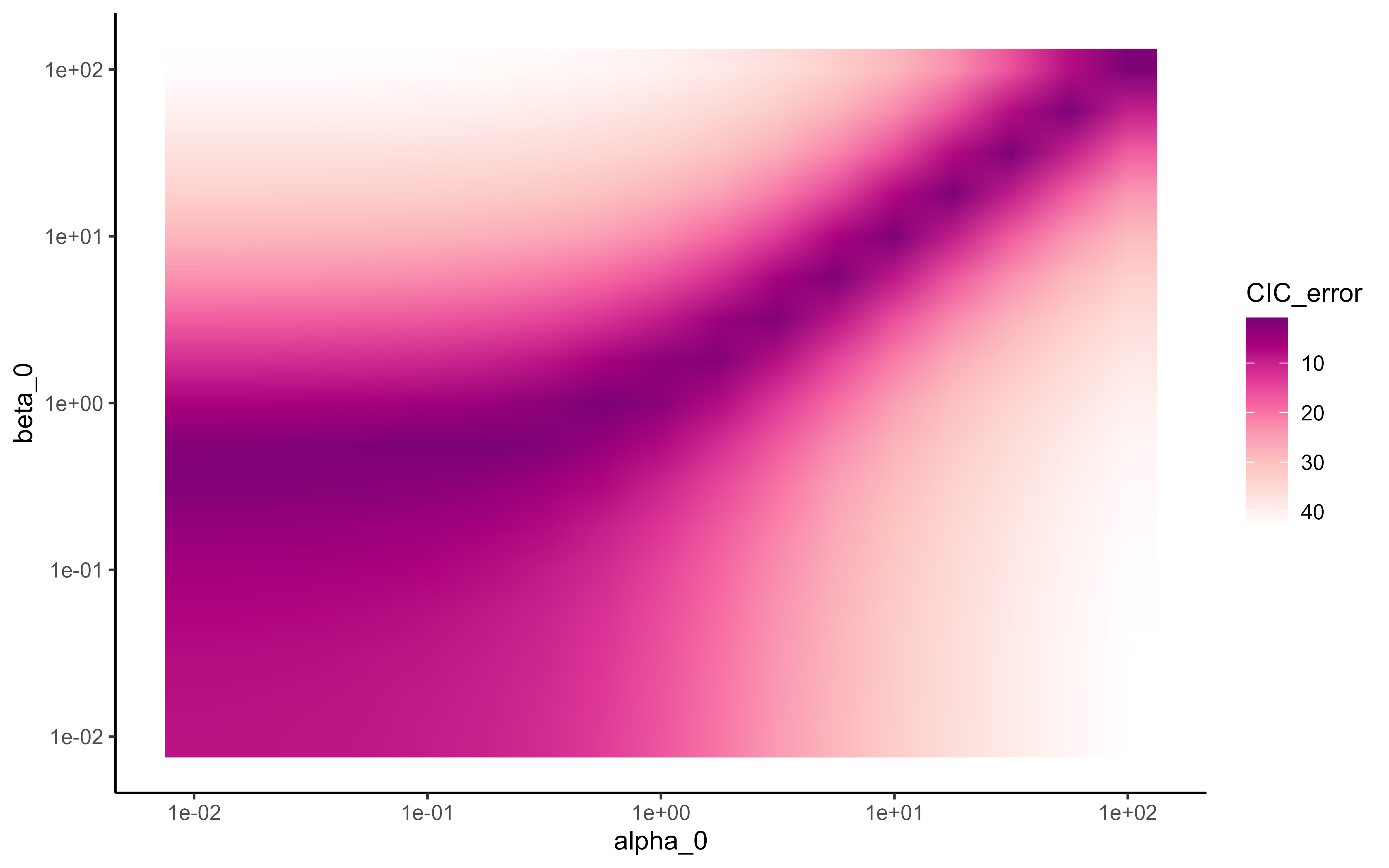
where represent the average of observed values computed over all groups. The values of and correspond to the empirical insights, as displayed in Figure 7, where errors in prior calibration of uncertainty appear to be minimal. The other hyperparameters are set to low informative values to minimise possible bias from the prior distribution in our empirical study. As previously stated, identical values in all groups are essential to ensure a fair and unbiased comparison. In the case where more expert information would be accessible, its incorporation would be possible, for instance, through the definition of a more precise prior mean () associated with a more confident prior variance (encoded through and ).
3.4 Performance metrics
We compared the performance of our method to the limma framework implemented in the ProStaR software through the DAPAR R package Wieczorek et al. (2017). However, due to the intrinsic difference in paradigm, limma being a frequentist tool and ProteoBayes a probabilistic one, we could only compare them in terms of mean difference recovery. To evaluate ProteoBayes as a probabilistic tool, we used other metrics, such as the credible interval width and the RMSE and credible interval coverage, to assess the quality of estimation.
-
•
Mean difference: For each peptide, we computed the difference between the mean intensity in the two groups compared. The common practice in proteomics uses log2-intensities instead of raw intensities. Therefore, the mean difference is similar to the log2-fold change.
-
•
95% Credible Interval Width (CI95 width): This indicator reflects the uncertainty in the posterior distribution of the mean. A smaller CIwidth denotes a more confident result in the estimated intensity mean. For each peptide, we computed the range between the bounds of the 95% credible interval.
-
•
Root Mean Square Error (RMSE): This indicator describes the average error for all peptides between the posterior intensity mean and the reconstructed reference intensity mean (see next paragraph).
-
•
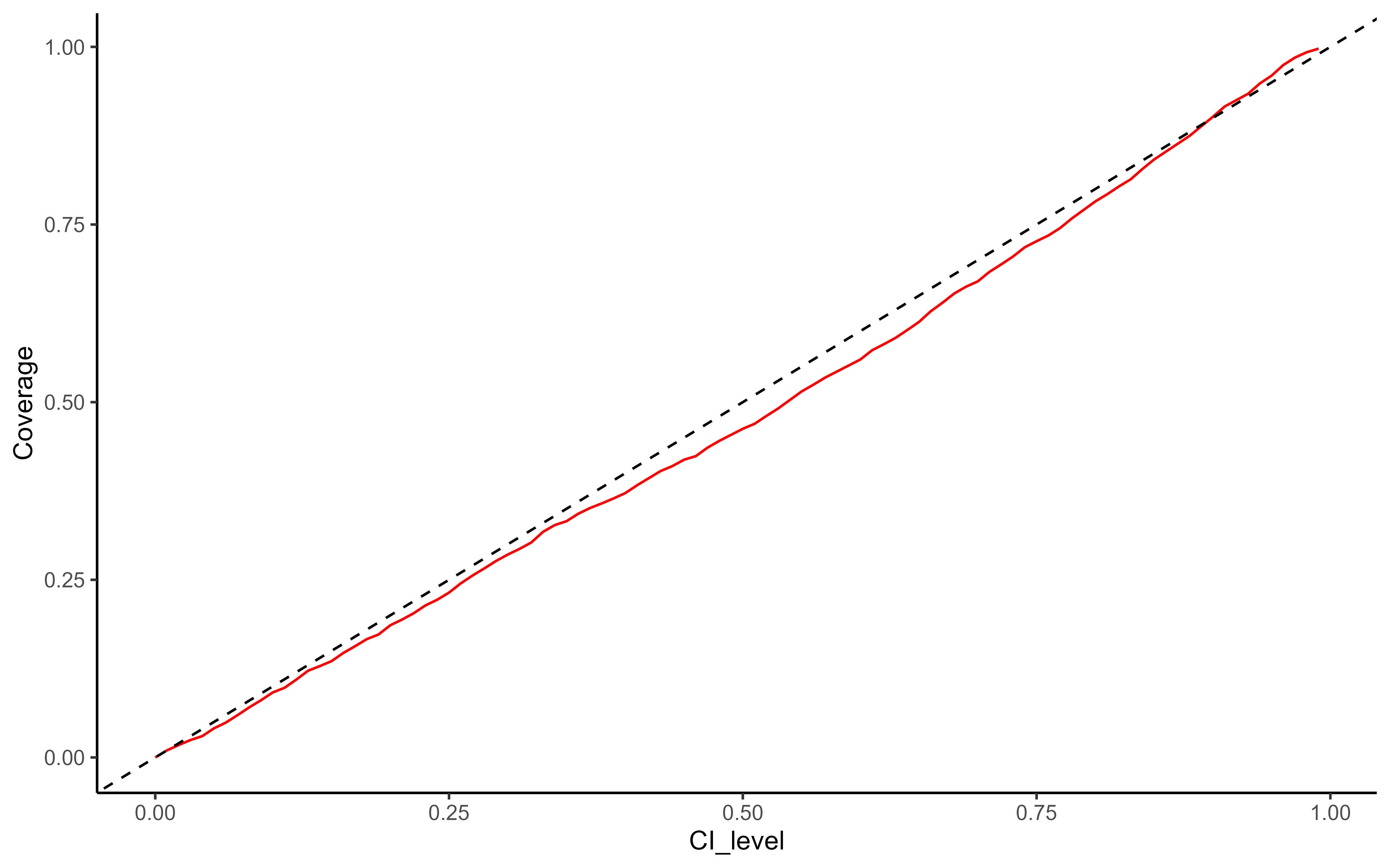
95% Credible Interval Coverage (CIC95): This indicator shows how well our method is calibrated and should have values around 95%. It is computed as the proportion of peptides for which the reference mean falls within the 95% credible interval bounds.
The RMSE and CIC95 indicators rely on a reference mean. Ideally, this would be the true mean intensity for each peptide within a group, but since that value is unknown, we need an alternative approach. Fortunately, the spike-in experimental design provides known theoretical abundances. In proteomics, global quantification assumes that peptide intensity is proportional to its quantity based on its response factor. This means that while we may not know the absolute mean intensity, we do know the true difference in mean intensity between two groups. For each group and each peptide , we reconstructed the reference intensity mean as follows:
-
1.
For each peptide, we adjusted its observed intensity by adding the log2-fold change between its group and a designated reference group (in the real data experiments, the highest point of the spike-in range). This created a reconstructed sample of peptide intensities for the reference group.
-
2.
We then averaged these reconstructed values to obtain the reference mean intensity for the reference group.
-
3.
Finally, for each peptide in any other group, we derived its reference mean intensity by subtracting the log2-fold change from the reference mean of the reference group.
3.5 Illustration and interpretation of posterior distributions
First, let us illustrate the univariate framework described in Section 2.3, using the Chion2022 dataset. In this experiment, we compared the intensity means in the lowest (0.05 fmol UPS1) and the highest points (10 fmol UPS1) of the UPS1 spike range. Remember that our univariate algorithm does not rely on imputation and should be applied directly to raw data. For the sake of illustration, the chosen peptides were observed entirely in all three biological samples of both experimental conditions.
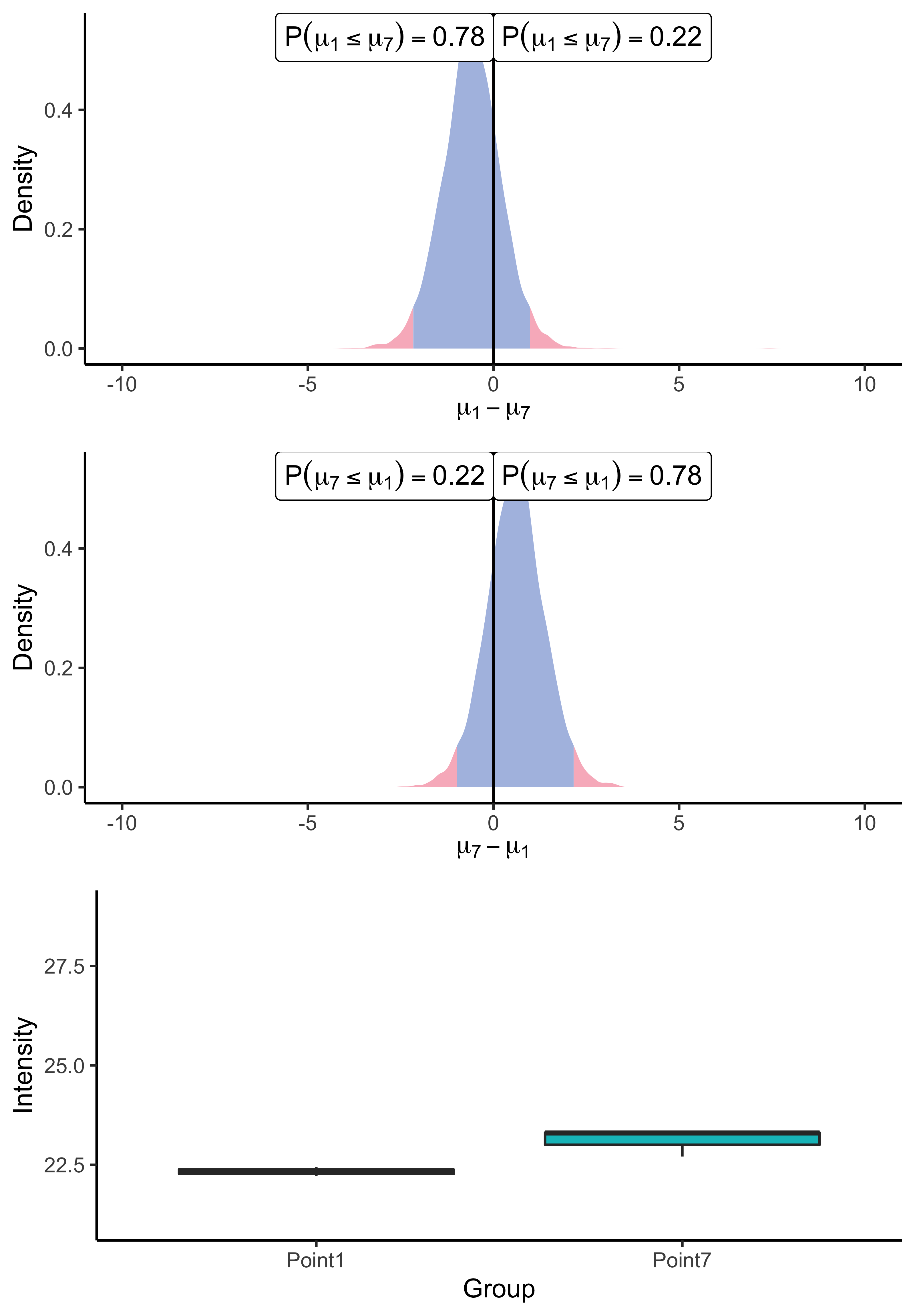
spF4I893ILA_ARATH protein.
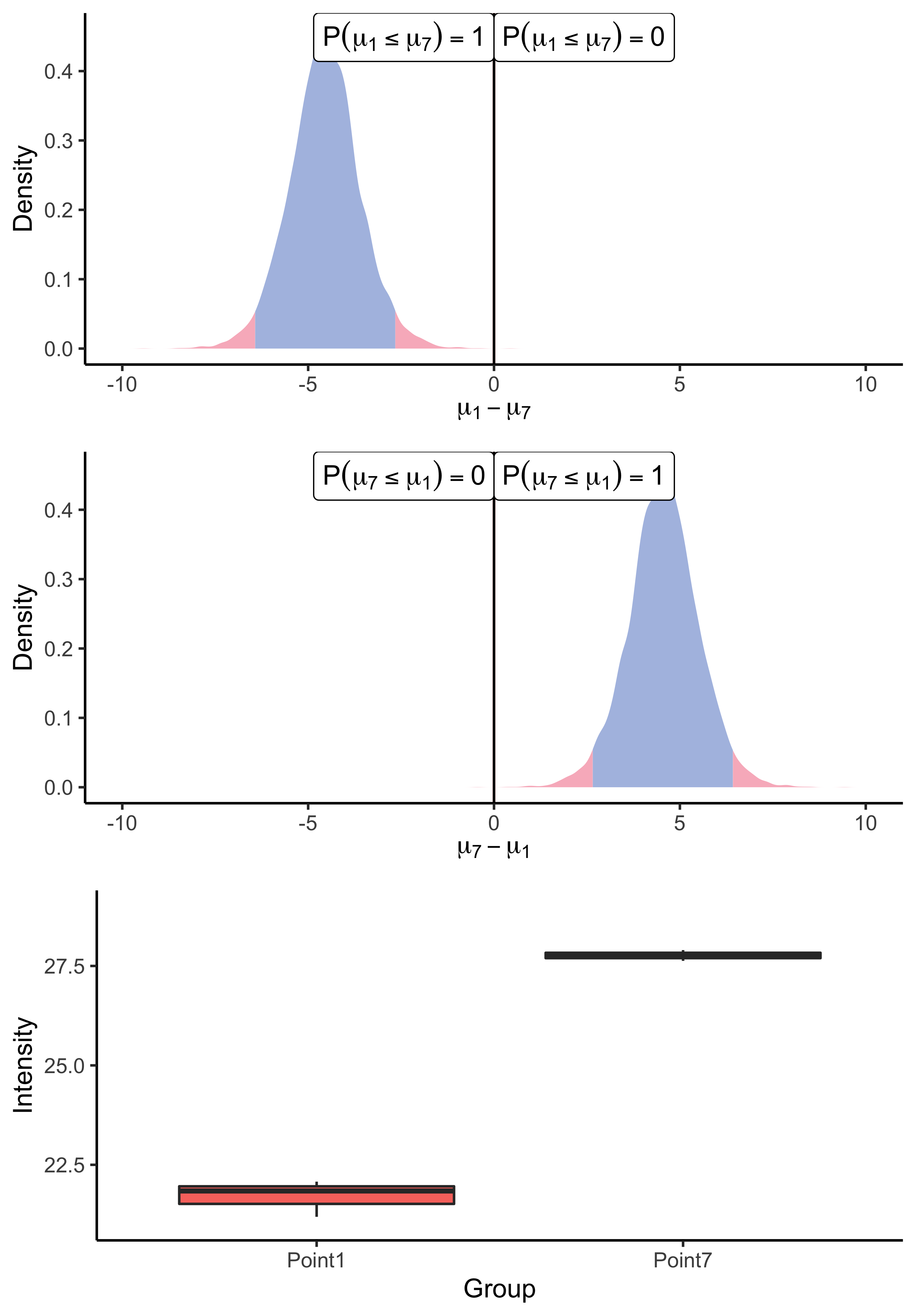
As a result of the application of our univariate algorithm, posterior distributions of the mean difference for both peptides are represented on Figure 3. As the analysis consists of a comparison between conditions, the 0 value has been highlighted on the x-axis to assess both the direction and the magnitude of the difference. The distance to zero of the distributions indicates whether the peptide is differentially expressed or not. In particular, Figure 3(a) shows the posterior distribution of the means’ difference for the UPS peptide. Its location, far from zero, indicates a high probability (almost surely in this case) that the mean intensity of this peptide differs between the two considered groups. Conversely, the posterior distribution of the difference of means for the ARATH peptide (Figure 3(b)) suggests that the probability that means differ is low. Those conclusions support the raw data summaries depicted on the bottom panel of Figure 3. Moreover, the posterior distribution provides additional insights into whether a peptide is under-expressed or over-expressed in a condition compared to another. For example, looking back to the UPS peptide, Figure 3(a) suggests an over-expression of the AALEELVK peptide in the seventh group (being the condition with the highest amount of UPS spike) compared to the first group (being the condition with the lowest amount of UPS spike), which is consistent with the experimental design. Furthermore, the middle panel merely highlights the fact that the posterior distribution of the difference is symmetric of , thus, the sense of the comparison only remains an aesthetic choice.
3.6 Univariate Bayesian inference for differential analysis
In this subsection, we evaluate the univariate framework described in Section 2.3 using the performance indicators defined in Section 3.4.
3.6.1 Running time comparison
A drawback that is often associated with Bayesian methods lies in the increasing computational burden compared to frequentist counterparts. However, by leveraging conjugate priors in our model and relying on sampling from analytical distributions to conduct inference, we managed to maintain a (univariate) algorithm as quick as t-tests in practice, as illustrated in Table 2. As expected, the multivariate version generally takes slightly longer to run as we need to estimate covariance matrices, which typically grow quickly with the number of peptides simultaneously modelled. That said, let us point out that we can still easily scale up to many thousands of peptides in a reasonable time (from a few seconds to minutes).
| ProteoBayes | t-test | limma | ||
|---|---|---|---|---|
| Univariate | Multivariate | |||
| 0.01 (0.01) | 0.22 (0.13) | 0.02 (0.01) | 0.03 (0.02) | |
| 0.05 (0.03) | 0.20 (0.08) | 0.07 (0.08) | 0.04 (0.02) | |
| 0.26 (0.02) | 0.95 (0.42) | 0.24 (0.06) | 0.09 (0.03) | |
| 3.17 (0.99) | 249.17 (27.51) | 2.64 (0.79) | 9.10 (6.34) | |
3.6.2 Acknowledging the effect size
ProteoBayes Quality of estimation t-test limma Mean difference width RMSE p-value p-value 5 samples 1.02 (0.62) 2.09 (0.63) 0.45 (0.53) 95.10 (21.60) 0.24 (0.26) 0.22 (0.26) 5.07 (0.63) 2.11 (0.62) 0.46 (0.54) 94.2 (23.39) 0 (0) 0 (0) 10.05 (0.61) 2.15 (0.65) 0.42 (0.50) 96.6 (18.34) 0 (0) 0 (0) 1.03 (2.34) 9.52 (3.48) 2.30 (2.88) 91.8 (27.45) 0.46 (0.29) 0.75 (0.18) 0.96 (4.59) 19.25 (6.62) 4.57 (5.38) 91.6 (27.75) 0.49 (0.29) 0.58 (0.26) 0.75 (8.96) 38.58 (13.98) 8.95 (10.95) 93.0 (10.95) 0.51 (0.29) 0.40 (0.31) 1000 samples 1 (0.04) 0.12 (0.003) 0.03 (0.04) 95.7 (20.3) 0 (0) 0 (0) 4.99 (0.04) 0.12 (0.003) 0.03 (0.04) 94.6 (22.61) 0 (0) 0 (0) 9.99 (0.04) 0.13 (0.003) 0.03 (0.04) 95.9 (19.84) 0 (0) 0 (0) 1 (0.16) 0.6 (0.01) 0.16 (0.19) 95.5 (20.74) 0 (0) 0.04 (0.04) 0.99 (0.31) 1.2 (0.02) 0.31 (0.37) 95.0 (21.81) 0.03 (0.08) 0.08 (0.12) 1.04 (0.58) 2.4 (0.06) 0.62 (0.75) 95.2 (21.39) 0.22 (0.26) 0.15 (0.24)
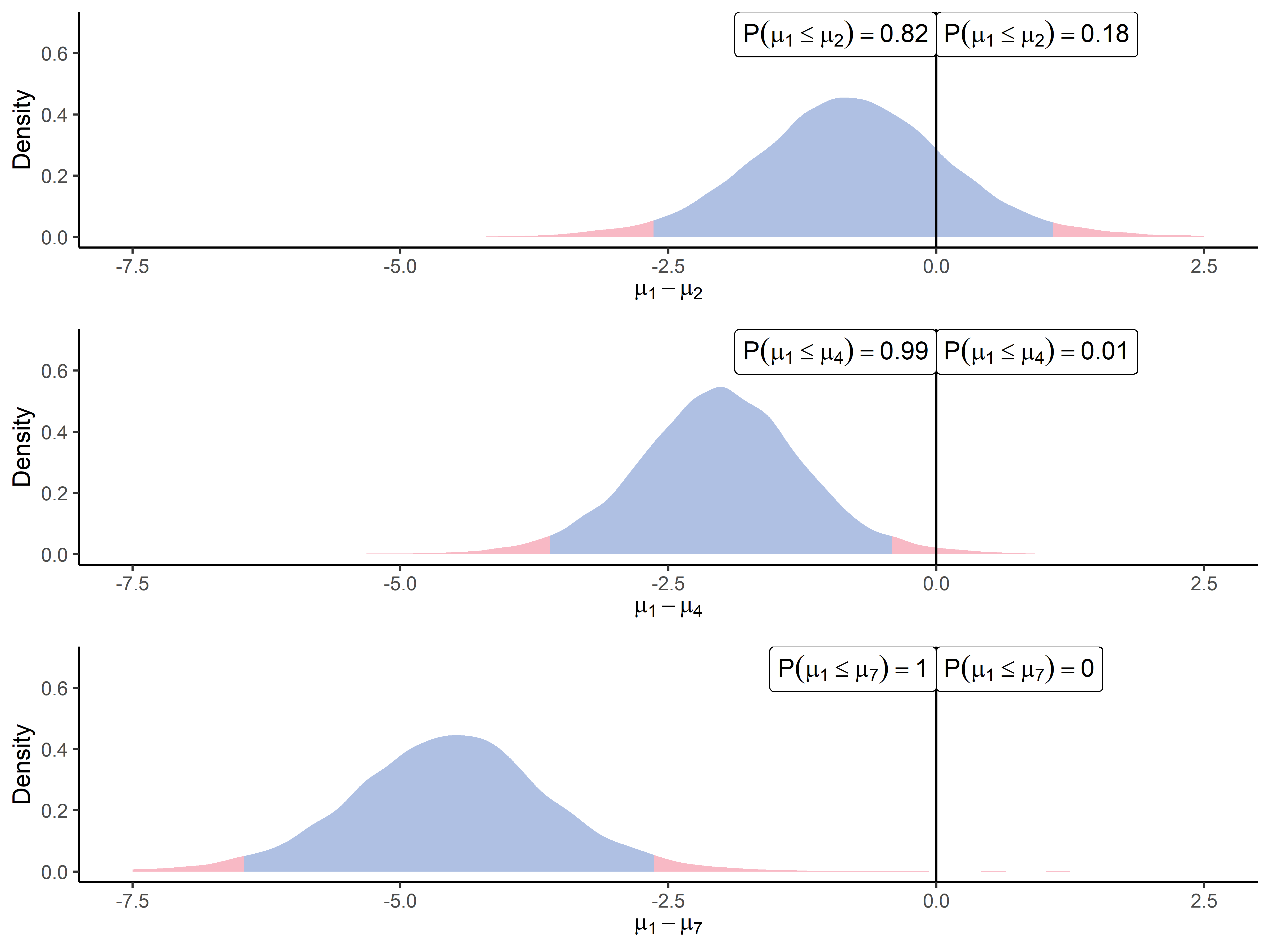
As highlighted in Figure 4, one key feature of ProteoBayes is its ability to naturally provide the effect size, i.e. the estimated difference between two groups (which is generally referred to as fold change in proteomics). The three panels describe the increasing differences that can be observed when we sequentially compare the first point (0.05 fmol UPS1) of the UPS1 spike range () to the second one (0.25 fmol UPS1 - ), the fourth one (1.25 fmol UPS1 - ) and the highest one (25 fmol UPS1 - ). The experimental design suggests that the difference in means for a UPS1 peptide should increase with respect to the amount of UPS proteins that were spiked in the biological sample (Chion et al., 2022). This illustration offers a perspective on how this difference becomes increasingly noticeable, though mitigated by the inherent variability. Such an explicit and adequately quantified variance, combined with the induced uncertainty in the estimation, should help practitioners make more educated decisions with the appropriate degree of caution. In particular, Figure 4 highlights the importance of considering the effect size (increasing here), which is crucial when studying the underlying biological phenomenon. Such a graph may remind us that statistical inference should be more about offering helpful insights to experts of a particular domain rather than defining automatic and blind decision-making procedures (Betensky, 2019). Moreover, let us point out that current statistical tests used for differential analysis express their results solely as -values. One should keep in mind that, no matter their value, they do not provide any information about the effect size of the phenomenon (Sullivan and Feinn, 2012).
To dive into the extensive evaluation of ProteoBayes on synthetic data, we provided in Table 3 a thorough analysis of mean differences computation for various effect size and variance combinations. We recover values that are remarkably close to the true mean difference on average in all cases. As expected, increasing the variance in the data would result in larger credible intervals are the computed posterior distributions adapt to the higher uncertainty context. Even though the literature often points out this issue, the p-values from the t-test in these experiments seem particularly uninformative in this context. Their values are so close to 0 that it is generally difficult to assess how much the two groups are close, with an adequate degree of caution. Moreover, these results were all computed for a sample size of 5 and 1,000. It is well known that p-values can change dramatically depending on sample size, regardless of the true underlying difference between groups.
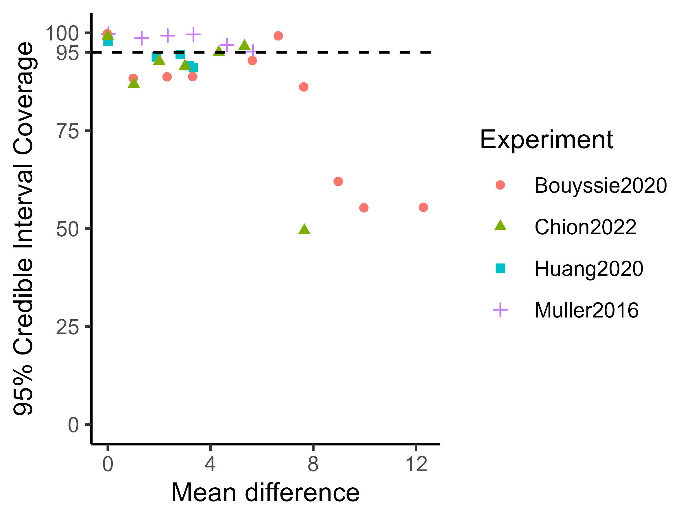
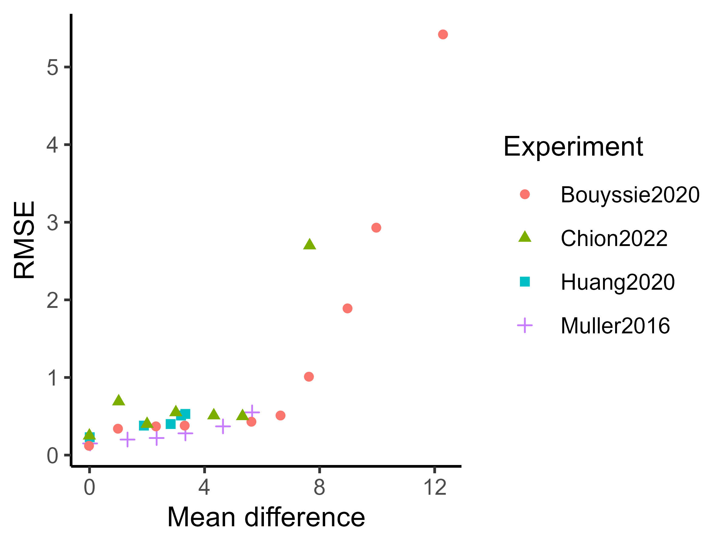
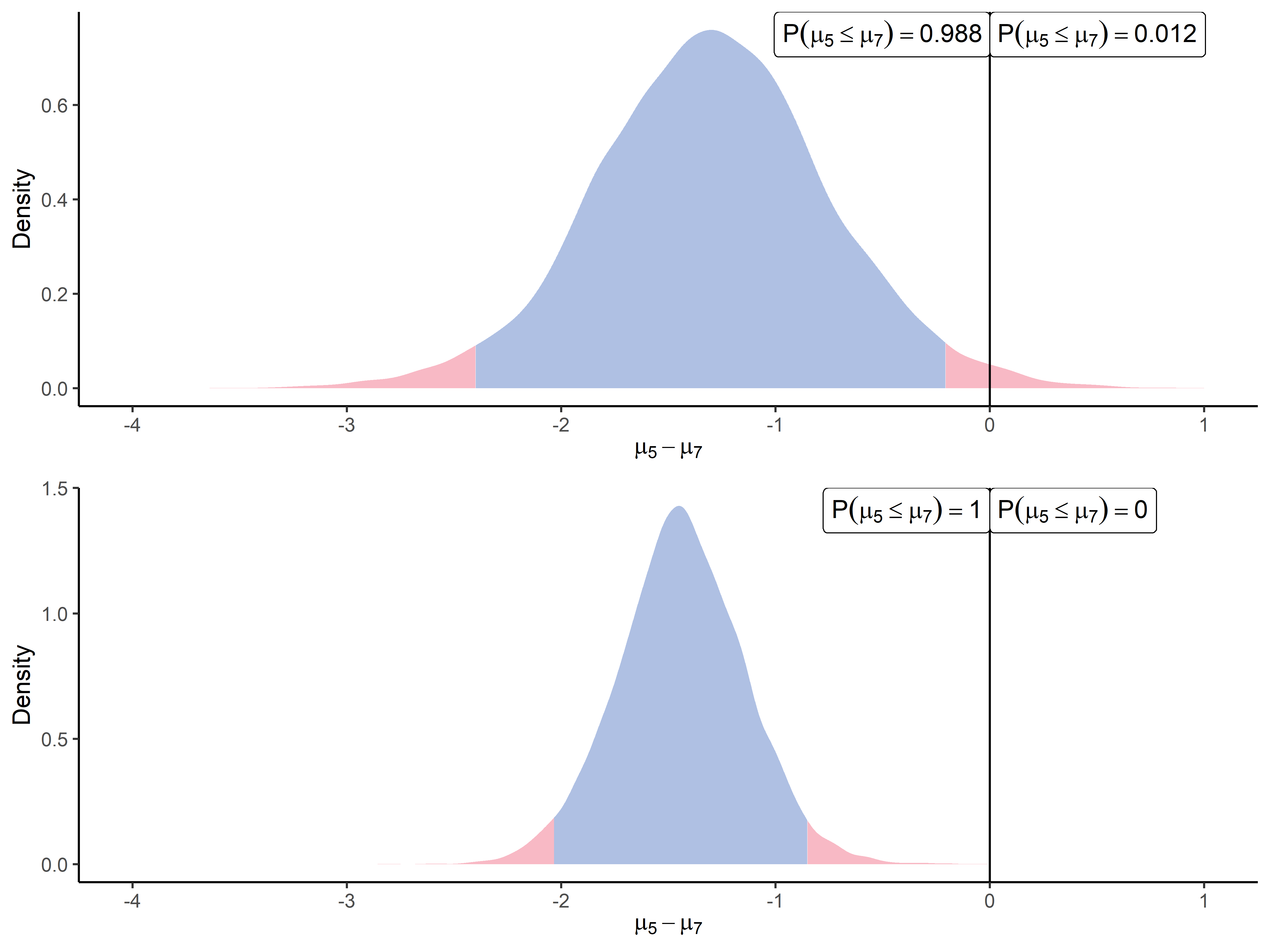
Experiments on real datasets are shown in Tables 4, 7, 8 and 9. While these experiments yield overall good results, there are some noticeable differences compared to the simulated results. As the absolute value of the true mean difference increases, the performance in terms of effect size recovery and uncertainty quantification decreases. In particular, the highest fold changes do not appear to be well recovered by either limma or ProteoBayes, as observed in the Bouyssie2020 and Chion2022 experiments Tables 7 and 9. This could challenge the proportionality hypothesis between the quantity of proteins and their measured intensities, see fig. 10.
Truth Vs. 25 fmol Nb of peptides Mean difference ProteoBayes True limma ProteoBayes CI95 width RMSE CIC95 UPS 0.5 fmol 229 -5.64 -5.01 (1.20) -5.01 (1.20) 7.72 (7.58) 0.92 (1.52) 95.20 (21.43) 1 fmol 350 -4.64 -4.31 (0.86) -4.31 (0.86) 6.08 (6.89) 0.57 (0.91) 96.86 (17.47) 2.5 fmol 478 -3.32 -3.09 (0.71) -3.09 (0.71) 5.06 (6.14) 0.47 (0.83) 99.58 (6.46) 5 fmol 538 -2.32 -2.18 (0.58) -2.18 (0.58) 4.18 (5.45) 0.39 (0.87) 99.26 (8.60) 10 fmol 585 -1.32 -1.20 (0.39) -1.20 (0.39) 2.94 (3.83) 0.32 (0.59) 98.63 (11.62) YEAST 0.5 fmol 19856 0 0.09 (0.45) 0.09 (0.45) 3.14 (4.01) 0.31 (0.74) 99.74 (5.11) 10 fmol 19776 0 0.04 (0.39) 0.04 (0.39) 3.17 (4.23) 0.28 (0.72) 99.70 (5.50) 1 fmol 19784 0 0.11 (0.43) 0.11 (0.43) 3.01 (3.98) 0.30 (1.04) 99.53 (6.80) 2.5 fmol 19835 0 0.10 (0.40) 0.10 (0.40) 3.20 (4.11) 0.27 (0.67) 99.83 (4.08) 5 fmol 19740 0 0.07 (0.38) 0.07 (0.38) 3.09 (4.08) 0.26 (0.66) 99.82 (4.21)
3.6.3 The mirage of imputed data
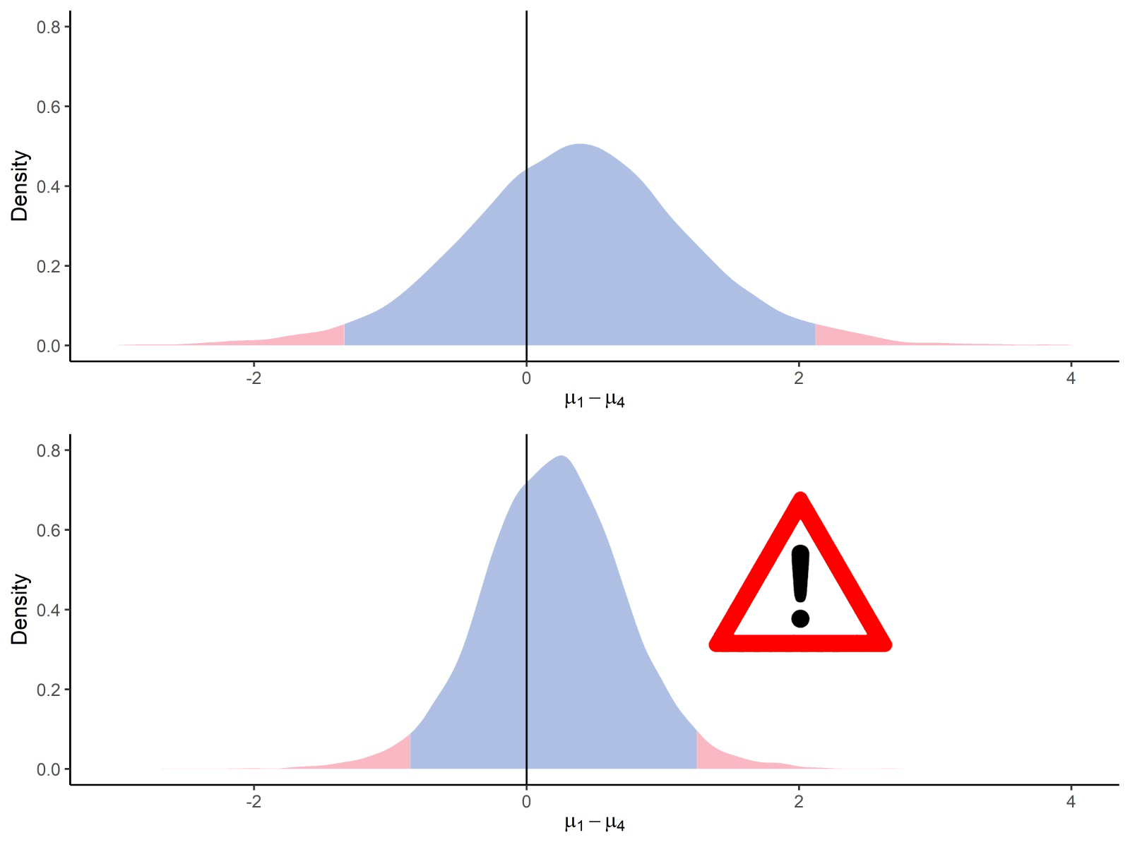
After discussing the advantages and the valuable interpretative properties of our methods, let us mention a pitfall that one should avoid for the inferences to remain valid. In the case of univariate analysis, we pointed out with Equation 3 that all the useful information is contained in observed data, and no imputation is needed since we already integrated out missing data. Imputation does not make sense in one dimension since, by definition, a missing data point is equivalent to an unobserved one, as we shall obtain more information only by collecting more data. Therefore, one should be careful when dealing with imputed datasets and remember that imputation creates new data points that do not bear any additional information. Thus, there is a risk of artificially decreasing the uncertainty of our estimated posterior distributions simply by considering more data points in the computations than what was genuinely observed. For the sake of illustration, let us assume a toy example where 10 points are effectively observed while 1000 remain missing. It would result in a massive underestimation of the actual uncertainty to impute 1000 missing points (say with the average of the ten observed ones) and use the resulting 1010-dimensional vector for computing posterior distributions of the mean. Let us mention that such a problem is not specific to our framework and, more generally, also applies to Rubin’s rules. Let us point out that those approximations only hold for a reasonable ratio of missing data. Otherwise, one may consider adapting the method, for example, by penalising the degree of freedom in the relevant -distributions. To illustrate this issue, we displayed in Figure 9 of the supplementary an example of our univariate algorithm applied both on the observed dataset (top panel) and the imputed dataset (bottom panel). In this context, we observe a reduced variance for the imputed data. However, this behaviour is just an artefact of the phenomenon mentioned above: the bottom graph is merely not valid, and only raw data should be used in our univariate algorithm to avoid spurious inference results. More generally, while imputation is sometimes needed for the methods to work, one should keep in mind that it always constitutes a bias (although controlled) that should be accounted for.
| Missing ratio | ProteoBayes | t-test p_value | limma p_value | |||
|
|
|||||
| Complete data | 0% | 1 (0.44) | 94.94 (21.92) | 1.35 (0.30) | 0.12 (0.18) | 0.11 (0.18) |
| 20% | 1 (0.51) | 94.74 (22.32) | 1.57 (0.44) | 0.16 (0.22) | 0.14 (0.22) | |
| No imputation | 50% | 0.99 (0.67) | 95.86 (19.91) | 2.32 (1.10) | 0.26 (0.27) | 0.24 (0.27) |
| 80% | 1 (0.91) | 97.56 (15.42) | 3.91 (1.88) | 0.37 (0.28) | 0.33 (0.30) | |
| 20% | 1 (0.48) | 88.96 (31.34) | 1.19 (0.31) | 0.10 (0.19) | 0.10 (0.19) | |
| Imputation | 50% | 1.01 (0.49) | 78.00 (41.43) | 0.93 (0.31) | 0.08 (0.18) | 0.07 (0.17) |
| 80% | 1 (0.48) | 61.34 (48.70) | 0.62 (0.25) | 0.04 (0.13) | 0.03 (0.12) |
3.7 Multivariate Bayesian inference
3.7.1 The benefit of intra-protein correlation
One of the main benefits of our methodology is to account for between-peptides correlation, as described in Section 2.2. As the first illustration of such a property, we modelled correlations between all quantified peptides derived from the same protein. In order to highlight the gains that we may expect from such modelling, we displayed on Figure 5 the comparison between a differential analysis using our univariate method or using the multivariate approach.
| Mean difference | width | ||
|---|---|---|---|
| Univariate | 0.92 (0.02) | 1.29 (0.03) | |
| 0.9 (0.03) | 1.69 (0.04) | ||
| Multivariate | 0.93 (0.02) | 0.93 (0.04) | |
| 0.89 (0.03) | 1.28 (0.06) |
In this example, we purposefully considered a group of 9 peptides coming from the same protein (P12081upsSYHC_HUMAN_UPS), which intensities may undoubtedly be correlated to some degree. We consider in this section the comparison of intensity means between the fifth point (2.5 fmol UPS - ) and the seventh point (10 fmol UPS - ) of the UPS spike range. The posterior difference of the mean vector between two conditions has been computed, and the first peptide (AALEELVK) has been extracted for graphical visualisation. Meanwhile, the univariate algorithm has also been applied to compute the posterior difference , solely on the peptide AALEELVK. The top panel of Figure 5 displays the latter approach, while the multivariate case is exhibited on the bottom panel. One should observe clearly that, while the location parameter of the two distributions is close as expected, the multivariate approach takes advantage of the information coming from the correlated peptides to reduce the uncertainty in the posterior estimation. To confirm this visual intuition, we provided in Table 6 additional evidence from synthetic datasets highlighting the tighter credible intervals obtained thanks to the multivariate modelling and accounting for inter-peptide correlations. This tighter range of probable values leads to a more precise estimation of the effect size and increased confidence in the resulting inference (deciding whether the peptide is differential or not).
3.7.2 About protein inference
To conclude on the practical usage of the proposed multivariate algorithm, let us develop ideas for comparing multiple peptides or proteins simultaneously.
As highlighted before, accounting for the covariances between peptides tends to reduce the uncertainty on the posterior distribution of a unique peptide.
However, we only exhibited examples comparing one peptide at a time between two conditions, although in applications, practitioners often need to compare thousands of them simultaneously.
From a practical point of view, while theoretically possible, we probably want to avoid modelling the correlations between every combination of peptides into a full rank matrix for at least two reasons.
First, it probably does not make much sense to assume that all peptides in a biological sample interact with no particular structure.
Secondly, it appears unreasonable to do so from a statistical and practical point of view.
Computing and storing a matrix with roughly rows and columns induces a computational and memory burden that would complicate the procedure while potentially leading to unreliable objects if matrices are estimated merely on a few data points, as in our example.
However, a more promising approach would consist of deriving a sparse approach by leveraging the underlying structure of data from a biological perspective.
If we reasonably assume, as before, that only peptides from common proteins present non-negligible correlations, it is then straightforward to define a block-diagonal matrix for the complete vector of peptides, which would be far more reasonable to estimate.
Such an approach would take advantage of both of our algorithms by using the factorisation (as in Equation 3) over thousands of proteins to sequentially estimate a high number of low-dimensional mean vectors.
Assuming an example with a thousand proteins containing ten peptides each, the approximate computing and storage requirements would be reduced from a order of magnitude (due to one high-dimensional matrix) to (a thousand small matrices).
In our applicative context, the strategy of dividing a big problem into independent smaller ones appears beneficial from both the applicative and statistical perspectives.
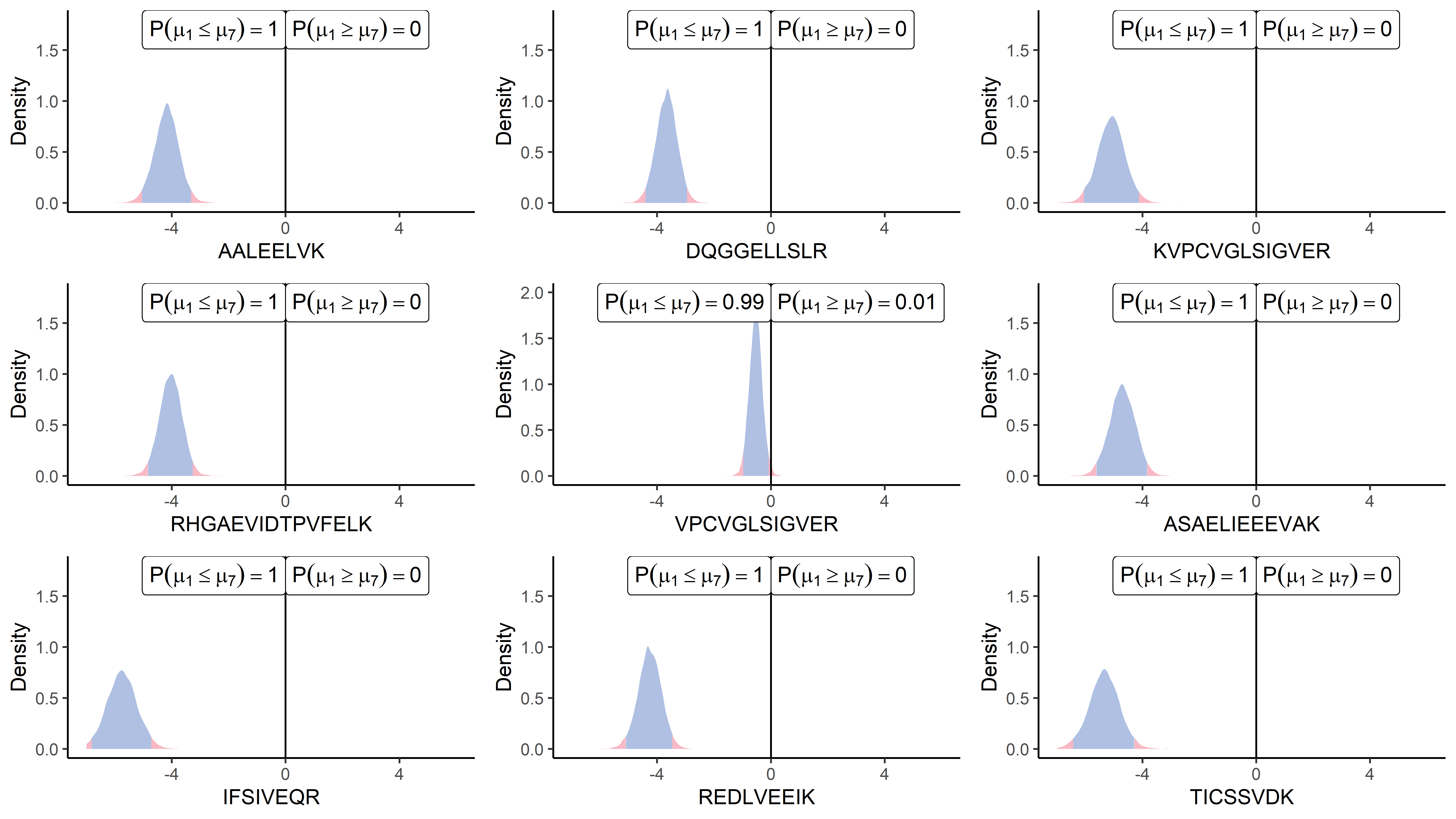
This being said, the question of the global inference, in contrast with a peptide-by-peptide approach, remains pregnant. To illustrate this topic, let us provide on Figure 6 an example of simultaneous differential analysis for nine peptides from the same protein. According to our previous recommendations, we accounted for the correlations through the multivariate algorithm and displayed the results in posterior means’ differences for each peptide from the P12081upsSYHC_HUMAN_UPS protein at once (i.e. ). In this example, eight peptides over nine contained in the protein are clearly differential in the same direction with comparable effect sizes, corroborating our intuition of correlated quantities. However, the situation may become far trickier when distributions lie closer to 0 on the x-axis or if only one peptide presents a clear differential pattern. As multiple and heterogeneous situations could be encountered, we do not provide recommendations here for directly dealing with protein-scale inference. Once again, the criterion for deciding what should be considered as different enough is highly dependent on the context and reasonable hypotheses, and no arbitrary threshold may bear any kind of general relevancy. However, we should still point out that our Bayesian framework provides convenient and natural interpretations in terms of probability for each peptide individually. It is then straightforward to construct probabilistic decision rules and combine them to reach a multivariate inference tool, for instance, by computing an average probability for the means’ difference to be below 0 across all peptides. However, one should note that probability rules prevent directly deriving global probabilistic statements without closely looking at dependencies between the single events (for instance, the factorisation in Equation 3 holds thanks to the induced independence between peptides). Although such an automatic procedure cannot replace expert analysis, it may still provide a handy tool for extracting the most noteworthy results from a massive number of comparisons, which the practitioner should look at more closely afterwards. Therefore, once a maximal risk of the adverse event or a minimum probability of the desired outcome has been defined, one may derive the adequate procedure to reach those properties.
4 Conclusion and perspectives
This article presents a Bayesian inference framework to tackle the problem of differential analysis in both univariate and multivariate contexts while accounting for possible missing data. We proposed two algorithms, leveraging classical results from conjugate priors to compute posterior distributions and easily sample the difference of means when comparing groups. To handle the recurrent problem of missing data, our multivariate approach takes advantage of the approximation of multiple imputations, while the univariate framework allows us to ignore this issue. In addition, this methodology aims to provide information not only on the probability of the means’ difference being null but also on the uncertainty quantification and effect sizes, which are crucial in a biological framework.
We believe that such probabilistic statements offer valuable inference tools to practitioners. In the particular context of differential proteomics, this methodology allows us to account for inter-peptide correlations. With an adequate decision rule and an appropriate correlation structure, Bayesian inference could be used in large-scale proteomics experiments, such as label-free global quantification strategies. Nevertheless, targeted proteomics experiments could already benefit from this approach, as the set of considered peptides is restricted. Furthermore, such experiments used in biomarker research could greatly benefit from the quantification of the uncertainty and the assessment of the effect sizes.
Code availability
The work described in the present article was implemented as an R package called ProteoBayes, available on CRAN, while a development version can be found on GitHub (https://github.com/mariechion/ProteoBayes). A companion web app can also be accessed at https://arthurleroy.shinyapps.io/ProteoBayes/.
Data availability
All simulated datasets and their generating code are available on Github (https://github.com/mariechion/ProteoBayes). All real datasets are public and accessible on the ProteomeXchange website using the following identifiers: PXD003841, PXD009815, PXD016647 and PXD027800.
5 Proofs
5.1 Proof of Bayesian inference for Normal-Inverse-Gamma conjugated priors
Let us recall below the complete development of this derivation by identification of the analytical form (we ignore conditioning over the hyperparameters for convenience):
Let us introduce Lemma 1 below to decompose the term as desired:
Lemma 1.
Assume a set , and note the associated average vector. For any :
Proof.
∎
Applying this result in our context for , we obtain:
5.2 Proof of General Bayesian framework for evaluating mean differences
Proof.
For the sake of clarity, let us omit the groups here and first consider a general case with . Moreover, let us focus on only one imputed dataset and maintain the notation for convenience. From the hypotheses of the model, we can derive , the posterior -PDF over , following the same idea as for the univariate case presented in Section 2.1:
By identification, we recognise the log-PDF that characterises the Gaussian-inverse-Wishart distribution with:
-
•
,
-
•
,
-
•
,
-
•
.
Once more, we can integrate over to compute the mean’s marginal posterior distribution by identifying the PDF of the inverse-Wishart distribution and by reorganising the terms:
The above expression corresponds to the PDF of a multivariate -distribution , with:
-
•
,
-
•
.
Therefore, we demonstrated that for each group and imputed dataset, the complete-data posterior distribution over is a multivariate -distribution. Thus, following Rubin’s rules for multiple imputation (see (Little and Rubin, 2019), we can propose an approximation to the true posterior distribution (that is only conditioned over observed values):
Leading to the desired results when evaluating the previously derived posterior distribution on each multiple-imputed dataset. ∎
References
- Ahlmann-Eltze and Anders (2020) Constantin Ahlmann-Eltze and Simon Anders. proDA: Probabilistic Dropout Analysis for Identifying Differentially Abundant Proteins in Label-Free Mass Spectrometry, May 2020.
- Betensky (2019) Rebecca A. Betensky. The p-Value Requires Context, Not a Threshold. The American Statistician, 73(sup1):115–117, March 2019. ISSN 0003-1305. doi: 10.1080/00031305.2018.1529624.
- Bishop (2006) Christopher M. Bishop. Pattern Recognition and Machine Learning. Springer, August 2006. ISBN 978-0-387-31073-2.
- Bolstad (2024) Ben Bolstad. preprocessCore: A collection of pre-processing functions. Bioconductor version: Release (3.20), 2024.
- Bouyssié et al. (2020) David Bouyssié, Anne-Marie Hesse, Emmanuelle Mouton-Barbosa, Magali Rompais, Charlotte Macron, Christine Carapito, Anne Gonzalez de Peredo, Yohann Couté, Véronique Dupierris, Alexandre Burel, Jean-Philippe Menetrey, Andrea Kalaitzakis, Julie Poisat, Aymen Romdhani, Odile Burlet-Schiltz, Sarah Cianférani, Jerome Garin, and Christophe Bruley. Proline: An efficient and user-friendly software suite for large-scale proteomics. Bioinformatics, 36(10):3148–3155, May 2020. ISSN 1367-4803. doi: 10.1093/bioinformatics/btaa118.
- Chang et al. (2018) Cheng Chang, Kaikun Xu, Chaoping Guo, Jinxia Wang, Qi Yan, Jian Zhang, Fuchu He, and Yunping Zhu. PANDA-view: An easy-to-use tool for statistical analysis and visualization of quantitative proteomics data. Bioinformatics, 34(20):3594–3596, October 2018. ISSN 1367-4803. doi: 10.1093/bioinformatics/bty408.
- Chion et al. (2022) Marie Chion, Christine Carapito, and Frédéric Bertrand. Accounting for multiple imputation-induced variability for differential analysis in mass spectrometry-based label-free quantitative proteomics. PLOS Computational Biology, 18(8):e1010420, August 2022. ISSN 1553-7358. doi: 10.1371/journal.pcbi.1010420.
- Choi et al. (2014) Meena Choi, Ching-Yun Chang, Timothy Clough, Daniel Broudy, Trevor Killeen, Brendan MacLean, and Olga Vitek. MSstats: An R package for statistical analysis of quantitative mass spectrometry-based proteomic experiments. Bioinformatics, 30(17):2524–2526, September 2014. ISSN 1367-4803. doi: 10.1093/bioinformatics/btu305.
- Colquhoun (2014) David Colquhoun. An investigation of the false discovery rate and the misinterpretation of p-values. Royal Society open science, 1(3):140216, 2014.
- Crook et al. (2022) Oliver M. Crook, Chun-wa Chung, and Charlotte M. Deane. Challenges and Opportunities for Bayesian Statistics in Proteomics. Journal of Proteome Research, 21(4):849–864, April 2022. ISSN 1535-3893. doi: 10.1021/acs.jproteome.1c00859.
- Dominici et al. (2000) Francesca Dominici, Giovanni Parmigiani, and Merlise Clyde. Conjugate Analysis of Multivariate Normal Data with Incomplete Observations. The Canadian Journal of Statistics / La Revue Canadienne de Statistique, 28(3):533–550, 2000. ISSN 0319-5724. doi: 10.2307/3315963.
- Etourneau et al. (2023) Lucas Etourneau, Laura Fancello, Samuel Wieczorek, Nelle Varoquaux, and Thomas Burger. A new take on missing value imputation for bottom-up label-free LC-MS/MS proteomics, November 2023.
- Huang et al. (2020) Ting Huang, Roland Bruderer, Jan Muntel, Yue Xuan, Olga Vitek, and Lukas Reiter. Combining Precursor and Fragment Information for Improved Detection of Differential Abundance in Data Independent Acquisition*. Molecular & Cellular Proteomics, 19(2):421–430, February 2020. ISSN 1535-9476. doi: 10.1074/mcp.RA119.001705.
- Ioannidis (2005) John PA Ioannidis. Why most published research findings are false. PLoS medicine, 2(8):e124, 2005.
- Kruschke (2013) John K. Kruschke. Bayesian estimation supersedes the t test. Journal of Experimental Psychology. General, 142(2):573–603, May 2013. ISSN 1939-2222. doi: 10.1037/a0029146.
- Kruschke and Liddell (2018) John K. Kruschke and Torrin M. Liddell. The Bayesian New Statistics: Hypothesis testing, estimation, meta-analysis, and power analysis from a Bayesian perspective. Psychonomic Bulletin & Review, 25(1):178–206, February 2018. ISSN 1531-5320. doi: 10.3758/s13423-016-1221-4.
- Lazar et al. (2016) Cosmin Lazar, Laurent Gatto, Myriam Ferro, Christophe Bruley, and Thomas Burger. Accounting for the Multiple Natures of Missing Values in Label-Free Quantitative Proteomics Data Sets to Compare Imputation Strategies. Journal of Proteome Research, 15(4):1116–1125, April 2016. ISSN 1535-3893. doi: 10.1021/acs.jproteome.5b00981.
- Little and Rubin (2019) Roderick Little and Donald Rubin. Statistical Analysis with Missing Data, Third Edition, volume 26 of Wiley Series in Probability and Statistics. Wiley, wiley edition, 2019. ISBN 978-0-470-52679-8.
- Muller et al. (2016) Leslie Muller, Luc Fornecker, Alain Van Dorsselaer, Sarah Cianférani, and Christine Carapito. Benchmarking sample preparation/digestion protocols reveals tube-gel being a fast and repeatable method for quantitative proteomics. PROTEOMICS, 16(23):2953–2961, 2016. ISSN 1615-9861. doi: 10.1002/pmic.201600288.
- Murphy (2007) Kevin Murphy. Conjugate Bayesian analysis of the Gaussian distribution, November 2007.
- O’Brien et al. (2018) Jonathon J. O’Brien, Harsha P. Gunawardena, Joao A. Paulo, Xian Chen, Joseph G. Ibrahim, Steven P. Gygi, and Bahjat F. Qaqish. The effects of nonignorable missing data on label-free mass spectrometry proteomics experiments. Annals of Applied Statistics, 12(4):2075–2095, December 2018. ISSN 1932-6157, 1941-7330. doi: 10.1214/18-AOAS1144.
- Smyth (2004) Gordon K Smyth. Linear Models and Empirical Bayes Methods for Assessing Differential Expression in Microarray Experiments. Statistical Applications in Genetics and Molecular Biology, 3(1):1–25, January 2004. ISSN 1544-6115. doi: 10.2202/1544-6115.1027.
- Sullivan and Feinn (2012) Gail M. Sullivan and Richard Feinn. Using Effect Size—or Why the P Value Is Not Enough. Journal of Graduate Medical Education, 4(3):279–282, September 2012. ISSN 1949-8349. doi: 10.4300/JGME-D-12-00156.1.
- The and Käll (2019) Matthew The and Lukas Käll. Integrated Identification and Quantification Error Probabilities for Shotgun Proteomics * [S]. Molecular & Cellular Proteomics, 18(3):561–570, March 2019. ISSN 1535-9476, 1535-9484. doi: 10.1074/mcp.RA118.001018.
- Tyanova et al. (2016) Stefka Tyanova, Tikira Temu, Pavel Sinitcyn, Arthur Carlson, Marco Y Hein, Tamar Geiger, Matthias Mann, and Jürgen Cox. The Perseus computational platform for comprehensive analysis of (prote)omics data. Nature Methods, 13(9):731–740, September 2016. ISSN 1548-7091, 1548-7105. doi: 10.1038/nmeth.3901.
- Wasserstein et al. (2019) Ronald L. Wasserstein, Allen L. Schirm, and Nicole A. Lazar. Moving to a World Beyond “p 0.05”. The American Statistician, 73(sup1):1–19, March 2019. ISSN 0003-1305. doi: 10.1080/00031305.2019.1583913.
- Wieczorek et al. (2017) Samuel Wieczorek, Florence Combes, Cosmin Lazar, Quentin Giai Gianetto, Laurent Gatto, Alexia Dorffer, Anne-Marie Hesse, Yohann Couté, Myriam Ferro, Christophe Bruley, and Thomas Burger. DAPAR & ProStaR: Software to perform statistical analyses in quantitative discovery proteomics. Bioinformatics (Oxford, England), 33(1):135–136, January 2017. ISSN 1367-4811. doi: 10.1093/bioinformatics/btw580.
6 Supplementary
Type Vs. 50 fmol Nb of peptides Mean difference ProteoBayes True limma ProteoBayes CI95 width RMSE CIC95 UPS 10 amol 101 -12.29 -5.49 (1.99) -5.49 (1.99) 11.47 (8.07) 5.58 (3.91) 55.45 (49.95) 50 amol 94 -9.97 -5.64 (1.96) -5.64 (1.96) 10.52 (8.20) 3.15 (2.68) 55.32 (49.98) 100 amol 108 -8.97 -5.88 (1.96) -5.88 (1.96) 10.71 (8.17) 2.19 (2.28) 62.04 (48.76) 250 amol 181 -7.64 -5.89 (1.81) -5.89 (1.81) 9.17 (8.04) 1.45 (2.17) 86.19 (34.60) 500 amol 252 -6.64 -5.86 (1.29) -5.86 (1.29) 7.95 (7.85) 0.76 (1.20) 99.21 (8.89) 1 fmol 351 -5.64 -5.20 (1.06) -5.20 (1.06) 6.20 (7.20) 0.64 (1.08) 92.88 (25.76) 5 fmol 545 -3.32 -3.25 (0.56) -3.25 (0.56) 3.62 (5.47) 0.66 (1.11) 88.81 (31.56) 10 fmol 623 -2.32 -2.26 (0.56) -2.26 (0.56) 2.79 (4.47) 0.71 (1.34) 88.76 (31.61) 25 fmol 680 -1 -0.99 (0.39) -0.99 (0.39) 2.02 (3.25) 0.69 (1.40) 88.38 (32.07) YEAST 10 amol 19739 0 0.12 (0.41) 0.12 (0.41) 2.89 (4.62) 0.23 (0.53) 99.75 (4.98) 50 amol 19776 0 0.13 (0.42) 0.13 (0.42) 2.74 (4.41) 0.24 (0.69) 99.69 (5.59) 100 amol 19749 0 0.14 (0.40) 0.14 (0.40) 2.72 (4.39) 0.22 (0.61) 99.78 (4.66) 250 amol 19770 0 0.14 (0.42) 0.14 (0.42) 2.76 (4.46) 0.23 (0.64) 99.76 (4.92) 500 amol 19852 0 0.16 (0.42) 0.16 (0.42) 2.74 (4.40) 0.23 (0.65) 99.83 (4.07) 1 fmol 19783 0 0.16 (0.41) 0.16 (0.41) 2.72 (4.38) 0.23 (0.57) 99.81 (4.38) 5 fmol 19768 0 0.14 (0.40) 0.14 (0.40) 2.73 (4.40) 0.23 (0.59) 99.76 (4.92) 10 fmol 19790 0 0.13 (0.38) 0.13 (0.38) 2.72 (4.40) 0.24 (0.64) 99.66 (5.81) 25 fmol 19632 0 0.06 (0.35) 0.06 (0.35) 2.83 (4.55) 0.25 (0.64) 99.67 (5.70)
Type Vs. 7.54 amol Nb of peptides Mean difference ProteoBayes True limma ProteoBayes CI95 width RMSE CIC95 UPS 0.75 amol 382 -3.33 -2.81 (1.77) -2.81 (1.77) 3.34 (4.46) 0.88 (1.62) 91.10 (28.51) 0.83 amol 382 -3.18 -2.82 (1.69) -2.82 (1.69) 3.45 (4.75) 0.86 (1.50) 91.62 (27.74) 1.07 amol 382 -2.82 -2.56 (1.51) -2.56 (1.51) 3.20 (4.66) 0.71 (1.25) 94.50 (22.82) 2.04 amol 390 -1.89 -1.74 (1.34) -1.74 (1.34) 2.63 (3.97) 0.65 (1.04) 93.85 (24.06) MOUSE 0.75 amol 95599 0 0.03 (0.78) 0.03 (0.78) 1.82 (2.41) 0.46 (1.27) 97.74 (14.86) 0.83 amol 95591 0 0.02 (0.78) 0.02 (0.78) 1.83 (2.46) 0.45 (1.15) 97.77 (14.76) 1.07 amol 95588 0 0.02 (0.77) 0.02 (0.77) 1.83 (2.46) 0.45 (1.21) 98.00 (14.00) 2.04 amol 95553 0 0.01 (0.77) 0.01 (0.77) 1.90 (2.54) 0.46 (1.17) 97.96 (14.14)
Type Vs. 10 fmol Nb of peptides Mean difference ProteoBayes True limma ProteoBayes CI95 width RMSE CIC95 UPS 0.05 fmol 205 -7.64 -4.21 (2.41) -4.21 (2.41) 7.64 (7.64) 3.20 (3.36) 49.76 (50.12) 0.25 fmol 350 -5.32 -4.59 (0.90) -4.59 (0.90) 6.44 (7.12) 0.72 (1.29) 96.29 (18.94) 0.5 fmol 459 -4.32 -3.52 (0.87) -3.52 (0.87) 4.71 (5.97) 0.65 (0.89) 94.99 (21.84) 1.25 fmol 539 -3 -3.06 (0.72) -3.06 (0.72) 4.82 (5.75) 0.72 (0.99) 91.47 (27.97) 2.5 fmol 608 -2 -1.7 (0.49) -1.7 (0.49) 3.35 (4.45) 0.58 (0.92) 92.76 (25.93) 5 fmol 618 -1 -1.43 (0.57) -1.43 (0.57) 3.69 (4.78) 0.88 (1.25) 86.89 (33.77) ARATH 0.05 fmol 15874 0 0.03 (0.60) 0.03 (0.60) 3.25 (4.37) 0.37 (0.77) 99.21 (8.84) 0.25 fmol 15879 0 0.06 (0.58) 0.06 (0.58) 3.12 (4.25) 0.35 (0.79) 99.31 (8.26) 0.5 fmol 15989 0 0.07 (0.56) 0.07 (0.56) 3.15 (4.25) 0.33 (0.93) 99.49 (7.10) 1.25 fmol 16397 0 0.08 (0.61) 0.08 (0.61) 3.74 (4.62) 0.45 (0.90) 98.33 (12.82) 2.5 fmol 16253 0 0.04 (0.46) 0.04 (0.46) 3.45 (4.61) 0.28 (0.80) 99.73 (5.20) 5 fmol 16228 0 0.03 (0.51) 0.03 (0.51) 3.88 (4.95) 0.48 (0.88) 98.24 (13.14)