A Bayesian theory for estimation of biodiversity
Abstract
Statistical inference on biodiversity has a rich history going back to RA Fisher. An influential ecological theory suggests the existence of a fundamental biodiversity number, denoted , which coincides with the precision parameter of a Dirichlet process (dp). In this paper, motivated by this theory, we develop Bayesian nonparametric methods for statistical inference on biodiversity, building on the literature on Gibbs-type priors. We argue that -diversity is the most natural extension of the fundamental biodiversity number and discuss strategies for its estimation. Furthermore, we develop novel theory and methods starting with an Aldous-Pitman (ap) process, which serves as the building block for any Gibbs-type prior with a square-root growth rate. We propose a modeling framework that accommodates the hierarchical structure of Linnean taxonomy, offering a more refined approach to quantifying biodiversity. The analysis of a large and comprehensive dataset on Amazon tree flora provides a motivating application.
1 Introduction
The decline in biodiversity represents a significant global concern, with potential implications for entire ecosystems and profound impacts on human well-being (e.g. Ceballos et al., 2015). Consequently, assessing diversity is a primary goal in ecology, although its practical measurement is a notoriously complex task (Colwell, 2009; Magurran and McGill, 2011). Taxon richness, the number of taxa within a community, is perhaps the simplest way to describe diversity, although alternative indices such as Simpson and Shannon indices, or Fisher’s , are often considered. The estimation of richness involves the analysis of taxon accumulation curves, a statistical methodology with roots that go back to the seminal work of Fisher et al. (1943), Good (1953), and Good and Toulmin (1956). Modern approaches are discussed in Bunge and Fitzpatrick (1993); Colwell (2009); Magurran and McGill (2011). See also Zito et al. (2023) for a recent model-based approach to analyzing accumulation curves and estimating richness.
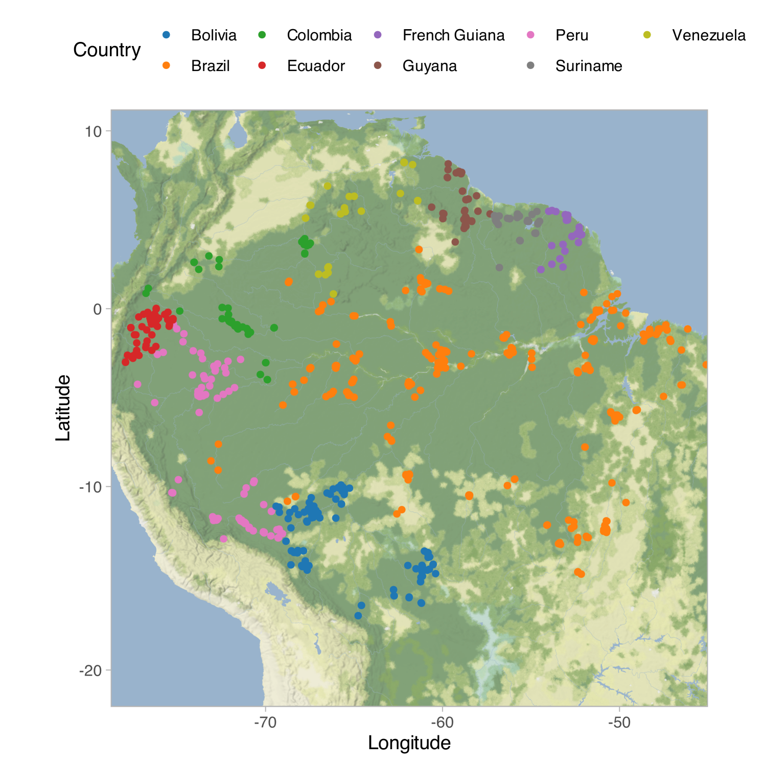
In an influential contribution, Hubbell (2001) postulated the existence of a fundamental biodiversity number , which lies at the core of his unified neutral theory of biodiversity. This number, , represents twice the population size multiplied by the speciation rate. The theory is conceptually attractive as it encapsulates biodiversity into a single number with a clear biological interpretation. In fact, is closely linked to accumulation curves, and Hubbell (2001) demonstrated that Fisher’s is asymptotically equivalent to the fundamental number for large population size values. The theory has found a successful application in predicting the number of tree species in the Amazon basin, as discussed in Hubbell et al. (2008) and ter Steege et al. (2013); the data are shown in Figure 1(a). These studies reported estimates of and for the fundamental biodiversity number, predicting approximately and tree species in the Amazon basin, respectively.
Interestingly, the fundamental biodiversity number in Hubbell’s theory corresponds to the precision parameter of a dp (Hubbell, 2001). The dp has been widely studied and has applications well beyond ecology and biodiversity (Hjort et al., 2010; Ghosal and Van der Vaart, 2017). Hubbell’s theory generated considerable controversy (e.g. McGill, 2003; Chisholm and Burgman, 2004; Ricklefs, 2006), being incompatible with data and ignoring mechanisms regarded important by ecologists (McGill, 2003). In fact, it is well known that dp is restrictive in depending on a single parameter and enforcing a logarithmic growth rate for the number of taxa (Lijoi et al., 2007a, b). To address these limitations, Gibbs-type priors have emerged as the most natural extension of the dp (Gnedin and Pitman, 2005; De Blasi et al., 2015) due to their balance between flexibility and tractability. This class includes the dp, Pitman-Yor process (Perman et al., 1992; Pitman and Yor, 1997), normalized inverse Gaussian process (Lijoi et al., 2005), and normalized generalized gamma process (Lijoi et al., 2007b).
We argue that the most natural generalization of Hubbell’s fundamental biodiversity number is the so-called -diversity of Pitman (2003). This retains the main appealing characteristic of the unified neutral theory, corresponding to the ability to describe biodiversity with a single interpretable number, while improving upon Hubbell by allowing for various growth rates for taxon accumulation curves. Classical estimation of -diversity is possible, but, as we shall see, the Gibbs-type framework naturally calls for Bayesian estimates. We contribute to the theory of Gibbs-type priors with novel statistical results and by pointing out connections among the classical work of Fisher et al. (1943), accumulation curves, and other measures of biodiversity. Moreover, we investigate in depth a Gibbs process we termed Aldous-Pitman after the work of Aldous and Pitman (1998); Pitman (2003), and we show that a suitable data-augmentation enables posterior inference.
Gibbs-type priors are natural tools for modeling biodiversity when focusing on a single level of the Linnean taxonomy, such as family, genus or species. However, each statistical unit often comprises a collection of different taxa, which are organized in a nested fashion; see, e.g., Zito et al. (2023). As a crude exemplification, one might consider using a different Gibbs-type model for each layer of the Linnean taxonomy. However, this approach would overlook the rich and informative nested structure of the data. Bayesian nonparametric models for such data are less developed. When , a sensible proposal is the enriched Dirichlet process (edp) of Wade et al. (2011), subsequently extended by Rigon et al. (2025) to the Pitman-Yor case. A more general prior with , and relying on a Pitman-Yor specification, is implicitly employed in Zito et al. (2023). We propose a general modelling structure that accounts for the complexities of the available data, focusing on the quantification of biodiversity. We call this novel approach taxonomic Gibbs-type priors, which combines the advantages of the enriched Dirichlet process of Wade et al. (2011) with the flexibility of Gibbs processes. In practice, this more refined approach results in taxon-specific indices of biodiversity that might be useful for comparing the biodiversity within branches of the taxonomic tree.
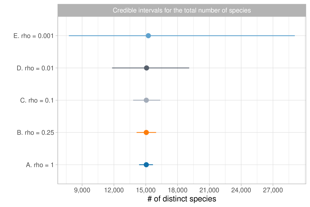
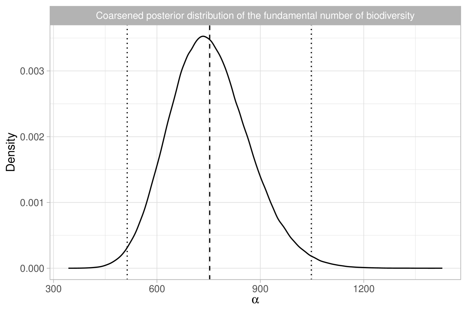
In Section 2, we discuss Bayesian nonparametric foundations of Hubbell (2001)’s theory of biodiversity. In Section 3 we use the Aldous-Pitman process to characterize biodiversity. In Section 4, we propose taxonomic Gibbs priors. In Section 5.1, we compare our Bayesian methodology with the analysis of ter Steege et al. (2013). As depicted in Figure 1(b), our estimate for is in close agreement with Hubbell et al. (2008) and ter Steege et al. (2013), with the benefit of uncertainty quantification. Bayesian inference for the number of tree species is also feasible, as will be discussed in Section 5.1. In Section 5.2, we analyze the Amazonian dataset more in-depth through our taxonomic Gibbs-type prior, providing new insights on the within-genera and within-family biodiversity.
2 Bayesian nonparametric modeling of taxon diversity
2.1 Gibbs-type priors
In this section, we provide an overview of Gibbs-type priors (Gnedin and Pitman, 2005), focusing on their relevance for ecological applications and quantification of biodiversity. For a mathematical exposition, we refer to De Blasi et al. (2015), while key theoretical developments are described in Lijoi et al. (2007a, b, 2008a, 2008b); De Blasi et al. (2013). Our data set comprises taxon labels , representing, for example, species or families, and taking values in a set . We assume that is an (ideally) infinite sequence of exchangeable observations which, according to the de Finetti theorem (de Finetti, 1937), is equivalent to the following hierarchical specification
| (1) | ||||
where is a (random) probability measure whose law is the prior distribution in Bayesian statistics. In our setting, we specify a multinomial model for , namely
| (2) |
where represents the Dirac delta measure at , whereas are random probability weights such that almost surely, and are random -valued locations, denoting distinct taxon labels. This approach is referred to as nonparametric because there are potentially infinitely many probabilities , for which a suitable prior will be specified. We assume that the ’s are iid samples from a diffuse probability distribution on and that and are independent. The diffuseness of implies that the labels ’s are all different. Thus, belongs to the class of proper species sampling models (ssms, Pitman, 1996). The baseline measure serves as a technical tool that simplifies the mathematical exposition, but we are not interested in “learning” it. Indeed, without loss of generality, in species sampling problems, we may let and let be a uniform distribution, meaning that each value is the numerical encoding of the associated taxon.
Remark 1.
The sampling mechanism in equation (1) makes explicit the assumptions behind species sampling models, of which Hubbell (2001)’s theory represents a special case. The core assumptions are: (i) ssms are tailored for the analysis of individual-based accumulation curves (Gotelli and Colwell, 2001) since the taxa are sampled sequentially, one at a time; (ii) taxon labels are independently sampled from (iid), implying that the probability of observing the th species remains constant across data points . These simplifying assumptions facilitate the definition of biodiversity indices, but are often violated in practice, particularly when analyzing meta-community data. For instance, observations may originate from different geographical regions, as in ter Steege et al. (2013), consequently leading to variations in the probability of observing a given taxon. Nevertheless, ssms serve as a useful approximation of reality, offering robust predictive capabilities, when a reasonable degree of homogeneity across observations is plausible.
The primary focus of inference typically lies not in the probabilities but rather in the combinatorial structure induced by the multinomial model of equation (2). Due to the discrete nature of , there will be identical values among with positive probability, comprising a total of distinct values with labels and frequencies such that . The random variable represents the observed taxon richness, whereas denote the associated abundances. The ties among the observations induce a random partition of the indices , where and . A species sampling model is a Gibbs-type process if the law of the random partition, called Gibbs partition, is such that
| (3) |
where denotes a rising factorial, is a discount parameter, and are non-negative weights satisfying the forward recursion for any and . is called the exchangeable partition probability function (eppf) and, in conjunction with , characterizes the distribution of random probability measure (Pitman, 1996). Of considerable importance is the predictive distribution induced by (Lijoi et al., 2007a):
| (4) |
The above predictive rule provides a sampling mechanism for the data . The term denotes the probability of discovering a new taxon, i.e., the probability of not being observed among the previous . Conversely, the probability corresponds to a Bayesian estimate of the sample coverage, namely the fraction of already observed taxa. The probability of re-observing the th taxon is proportional to , explaining why is sometimes referred to as the “discount parameter”, as it diminishes (or augments) the observed frequencies. Notable Gibbs-type priors are discussed below.
Example 1 (Dirichlet–multinomial, case ).
Consider , and let . A valid set of Gibbs coefficients is defined as:
| (5) |
where denotes the indicator function. This model assumes a finite number of taxa at a population level because the in-sample species richness is upper-bounded by . Its predictive scheme is:
Thus, the probability of discovering a new taxon is zero whenever . The corresponding process is called Dirichlet-multinomial, denoted by , with .
Example 2 (Dirichlet process, case ).
For and , a valid set of Gibbs coefficients is:
| (6) |
The corresponding process is the Dirichlet process of Ferguson (1973), with precision parameter , the fundamental biodiversity parameter of Hubbell (2001). The general predictive rule in (4) becomes:
the Blackwell and MacQueen (1973) urn scheme. The Dirichlet process admits a stick-breaking representation (Sethuraman, 1994): with and for , with . This highlights that (i) the dp assumes infinitely many taxa at a population level, and (ii) the probabilities of these taxa decrease exponentially fast at a rate determined by .
Example 3 (-stable Poisson-Kingman process, case ).
For and , we have
| (7) |
where is the gamma function and represents the density of a -stable distribution. The corresponding process is a -stable Poisson-Kingman (pk) process, conditional on “total mass” (Kingman, 1975; Pitman, 2003). The distribution of the associated probability weights is complex, but implies infinitely many species.
Remarkably, the aforementioned set of weights , and form the foundation of any Gibbs-type prior. In fact, Gibbs partitions can always be expressed as a mixture with respect to the parameters , , and . This result was established by Gnedin and Pitman (2005).
Proposition 1 (Gnedin and Pitman (2005)).
The Gibbs coefficients satisfy the recursive equation for any and in the following three cases:
-
1.
If , whenever , for some discrete random variable with probability distribution function , where the ’s are defined as in equation (5).
-
2.
If , whenever , for some positive random variable with probability measure , where the ’s are defined as in equation (6).
-
3.
If , whenever , for some positive random variable with probability measure , where the ’s are defined as in equation (7).
Any Gibbs-type process can be represented hierarchically, involving a suitable prior distribution for the key parameters , , and . Prior distributions for in the case are discussed in Gnedin (2010) and De Blasi et al. (2013); see also Miller and Harrison (2018) for applications to mixture models and Legramanti et al. (2022) for employment in stochastic block models. In the case, a popular choice is the semi-conjugate Gamma prior for as in Escobar and West (1995), with the Stirling-gamma prior of Zito et al. (2024) a recent alternative. Finally, in the regime, a polynomially tilted stable distribution prior for leads to the Pitman-Yor process (Pitman and Yor, 1997), whereas an exponentially tilted stable density leads to the normalized generalized gamma process (Lijoi et al., 2007b); refer to Lijoi et al. (2008b); Favaro et al. (2009) for a thorough investigation and to Favaro et al. (2015) for a general class of priors for .
2.2 The quantification of biodiversity
The simplest measure of biodiversity is arguably the taxon richness. In our notation, we observe different taxa among data points ; we refer to this value as the in-sample richness. A priori, the distribution of induced by a Gibbs-type prior has a simple form
where denotes a generalized factorial coefficient (Charalambides, 2002); the case is recovered as the limit of the above formula, since , which is the signless Stirling number of the first kind. The expected values can be interpreted as a model-based rarefaction curve (Zito et al., 2023). Moreover, we may want to predict the number of new taxa within a future sample ; we call this value the out-of-sample richness. The posterior distribution of given the data , or equivalently of the number of previously unobserved taxa , has been derived by Lijoi et al. (2007a) and is
where the term is the noncentral generalized factorial coefficient; see Lijoi et al. (2007a). The collection represents a model-based extrapolation of the accumulation curve. Note that is a sufficient statistic for predictions.
Example 4 (Dirichlet-multinomial, cont’d).
For the Dirichlet-multinomial, the rarefaction curve is
as shown in Pitman (2006, Chap. 3). Moreover, in the Appendix we provide a simple proof to show that:
Example 5 (Dirichlet process, cont’d).
In the Dirichlet process case, the rarefaction and the extrapolation curves are given by:
For their practical implementation, one can use for any , where is the digamma function. See, for example, Zito et al. (2023).
While rarefaction and extrapolation curves are valuable tools (Gotelli and Colwell, 2001), it is useful to summarize biodiversity with a single number. The concept of richness, defined as , is problematic since for regardless of the observed data, whereas remains finite for . Avoiding is tempting, but leads to poor fit and predictions for some datasets. Gibbs-type priors with positive often excel in predicting future values for highly diverse taxa, compared to models with (Lijoi et al., 2007a; Favaro et al., 2009). Additionally, the total number of taxa present in a given area can be estimated even in models where , e.g. following the strategy of ter Steege et al. (2013). This discussion motivates embracing an alternative concept of diversity, called -diversity, introduced by Pitman (2003), which encompasses Hubbell (2001)’s fundamental biodiversity number when .
Proposition 2 (-diversity, Pitman (2003)).
Let be the number of distinct values arising from a Gibbs-type prior in (3):
-
1.
Let and be defined as in equation (5), then almost surely;
-
2.
Let and be defined as in equation (6), then almost surely;
-
3.
Let and be defined as in equation (7), then almost surely.
For a generic set of weights , let be a function such that if , if , and if . Then as
| (8) |
The random variable is called -diversity and its distribution coincides with the prior for , and , respectively, implied by the mixture representation of the weights in Proposition 1.
The -diversity can be seen as a richness measure that has been appropriately rescaled. Proposition 2 highlights the central role of the Dirichlet-multinomial, Dirichlet, and -stable pk processes among Gibbs-type priors. It shows that their parameters , , and are biodiversity indices. In these three processes, diversity is deterministic and assumed to be known. However, -diversities , , or are typically unknown, and can be estimated employing a prior distribution, leading to a Gibbs-type process for thanks to Proposition 1. In light of this, the posterior law of -diversity is a key quantity for measuring biodiversity. In addition, the posterior distribution of has an elegant connection with accumulation curves, as shown in the following theorem.
Theorem 1.
Let be a sample from a Gibbs-type prior (3) with distinct values and let the function be defined as in Proposition 2. Then as
| (9) |
The random variable is the -diversity and its distribution coincides with the posterior for , and , respectively. Moreover, is a sufficient statistic for given the data .
Theorem 1 states that the posterior law of coincides with the -diversity associated with extrapolation of the accumulation curve. Related results for the normalized generalized gamma model are in Favaro et al. (2012). In practice, deriving the posterior distribution of -diversities , and is based on the Bayes theorem, where the eppf in (3) acts as likelihood function. Notably, in Gibbs-type priors, the abundances appearing in (3) do not provide insights about the diversity, and they do not appear in the posterior for because the number of observed species is a sufficient statistic. This would not be the case for general species sampling models beyond the Gibbs-type.
Example 6 (Dirichlet-multinomial, cont’d).
Bayesian inference for the richness , i.e. the case, is based on the posterior distribution
where denotes a discrete prior distribution for . If the prior has bounded support, sampling from the posterior is trivial. In general, acceptance-rejection or truncation strategies can be considered. When , shifted geometric and shifted Poisson prior specifications have been investigated in De Blasi et al. (2013), whereas Gnedin (2010) proposed a heavy-tailed prior distribution, which leads to a closed-form expression for the posterior distribution of and the weights .
Example 7 (Dirichlet-process, cont’d).
Bayesian inference about the fundamental biodiversity number , i.e. the case, is based on the posterior distribution
where denotes the prior distribution for . As noted in Zito et al. (2023), this problem is equivalent to a logistic regression with an offset. The choice has been advocated by Escobar and West (1995) because it leads to a semi-conjugate Gibbs-sampling scheme. More recently, Zito et al. (2024) proposed the (asymptotically equivalent) Stirling-gamma prior, which has the advantage of being highly interpretable, especially within the context of species sampling models.
Remark 2.
The discount parameter characterizes the asymptotic behavior of the Gibbs partition. Although one could theoretically estimate from data using a prior distribution, leading to a species sampling model beyond the Gibbs type, we argue that the choice of should be regarded as a model selection problem. This avoids difficulties in interpretation, since comparing -diversities across locations makes sense only if they are based on the same asymptotic regime. In practice, based on the data, can be chosen from the following values: (Dirichlet distribution with uniform weights), (Dirichlet process) and (Aldous-Pitman process).
Remark 3.
Fisher’s (Fisher et al., 1943) is an estimator for the parameter of the Dirichlet process (Hubbell, 2001). We compare Fisher’s with the maximum likelihood estimator of the diversity, with these estimators solving
For large , the two estimates are nearly identical, due to the inequalities (see, e.g., Ghosal and Van der Vaart, 2017, Proposition 4.8). This striking similarity between and results because the eppf of a Dirichlet process can be regarded as a conditional likelihood for Fisher’s model, in which the sample size is fixed and not random, contrary to Fisher’s original formulation; see McCullagh (2016) for a detailed historical account and further considerations. Hence, the posterior law of provides a Bayesian Fisher’s . The Bayesian perspective not only establishes an insightful link between Fisher’s and accumulation curves through Proposition 2 and Theorem 1, but also facilitates uncertainty quantification and testing.
2.3 Relationship between -diversity and other biodiversity measures
We show that many classical biodiversity indices can be expressed in terms of , , or , based on the connection with the accumulation curves discussed earlier. Consider the popular Simpson similarity index (e.g., Colwell, 2009), which is the probability that two randomly chosen individuals belong to the same taxa. Within the framework of species sampling models, and due to exchangeability In Gibbs-type priors, it follows that . We can specialize this formula in the Dirichlet multinomial and Dirichlet process case, yielding respectively
Thus, there is an inverse relationship between the expected Simpson similarity and the -diversity. The following section shows a similar relationship in the polynomial regime, when . More generally, most biodiversity indices can be expressed as for some function . For instance, corresponds to the Simpson index, is the Shannon diversity, and for some is the (unnormalized) Tsallis or Hill diversity (Colwell, 2009; Magurran and McGill, 2011). The expectations are a function of and . Additionally, their relationship with can often be explicitly determined: if the random probabilities are in size-biased order, then we have the simplification . For example, in the dp case, the stick-breaking weights are in size-biased order, and we have , which makes computations straightforward.
2.4 Model validation
We propose two approaches to assess the fit of the model. The first approach compares the observed distinct values with the model-based rarefaction curve . As shown above, expectations can often be computed explicitly, and are typically evaluated given an estimate for the diversity parameter, e.g. in the case. Due to exchangeability, expectations do not depend on the order of the data. However, in most cases, the data are not observed in a specific order. Thus, a common practice is to reshuffle the order of and then consider the averages , over all possible permutations of the data. Conveniently, for this combinatorial problem, there exists an explicit solution, which is:
where and are the abundances; see Smith and Grassle (1977); Colwell et al. (2012). The values define the “classical rarefaction”, which can be regarded as a frequentist nonparametric estimator arising from a multinomial model. Our Bayesian nonparametric approach instead depends on a few parameters, imposing some rigidity on the functional shape of the rarefaction, which is critical for extrapolation. Graphically comparing with can give a sense of the suitability of the chosen model. We show a concrete example in Section 5.1.
The second model-checking approach is even simpler and has been used, e.g. in Favaro et al. (2021); see also Thisted and Efron (1987) for early ideas. The abundances can be reformulated in terms of frequency counts , where is the number of taxa appearing with frequency in the sample. Hence, represents the number of singletons, is the number of doubletons, etc. We denote by the associated random variables. To assess goodness of fit, we compare empirical counts with their model-based expectations . In the Dirichlet process case, these expectations have a simple analytical formula
and therefore when , corresponding to the expected singletons implied by Hubbell (2001) theory, we get . The general analytical formulas for the expectations for any prior of Gibbs type are given in Favaro et al. (2013). These expectations can be approximated via Monte Carlo, by sampling from the urn scheme in equation (4).
3 The Aldous-Pitman process ()
The Dirichlet multinomial and Dirichlet process cases, corresponding to , have been extensively investigated in Bayesian nonparametrics. There exist suitable priors and well-established estimation procedures for and , as discussed in Section 2. In contrast, relatively less attention has been devoted to the case , which corresponds to rapidly growing accumulation curves, with notable exceptions such as Lijoi et al. (2007b) and Favaro et al. (2009). The main mathematical challenge lies in the density in equation (7), which lacks a simple analytical expression. However, in the case, this density becomes , significantly simplifying the calculations. This leads to the definition of what we term the Aldous-Pitman process.
Definition 1 (Aldous-Pitman process).
Let , and be a diffuse probability measure on . Additionally, let be iid samples from and and be iid samples from a standard Gaussian distribution. Define a species sampling model where
and . We will say that follows an Aldous-Pitman process with parameters and .
The Aldous-Pitman process, introduced by Aldous and Pitman (1998), is a special case of the -stable pk process described in Example 3, when (Pitman, 2003). Consequently, the Aldous-Pitman process results in a Gibbs partition, where the parameter corresponds to the -diversity. Notably, the weights satisfy , where represents the cumulative probability of rare taxa, which is directly influenced by the -diversity parameter . Furthermore, the associated Gibbs-type coefficients can be explicitly obtained.
Example 8 (Aldous-Pitman process, case ).
Suppose and let . Then a valid set of Gibbs coefficients is given by
| (10) |
where denotes the Hermite function of order (Lebedev, 1965, §10.2). The corresponding process is an Aldous-Pitman process, and the -diversity is . Moreover, the associated urn-scheme is as follows:
It can be shown (Pitman, 2003) that the expected Simpson index of an Aldous-Pitman process is
revealing the close relationship between the -diversity and the Simpson index.
The ap process serves as a building block for Gibbs-type priors with growth rate , having a -diversity . So far, two specific priors for have been investigated: the prior implicitly utilized in the Pitman–Yor process (Favaro et al., 2009) and the one implied by the normalized generalized gamma (ngg) process (Lijoi et al., 2007b). Both options yield tractable Gibbs coefficients for all values of . Furthermore, when these priors reduce to the following specifications
| (Pitman-Yor) | (11) | |||||
| (Normalized inverse Gaussian) |
where and are hyperparameters, and the densities for are given by and , for the Pitman-Yor and the inverse Gaussian case, respectively. These results can be deduced from Favaro et al. (2009) and Lijoi et al. (2005, 2007b). When the ngg process is also known as the normalized inverse Gaussian process (Lijoi et al., 2005).
The prior distributions in (11) are somewhat restrictive since, by fixing the asymptotic regime to , there is a single parameter ( or ) controlling the prior mean and variance for the -diversity. Here, we consider a generic prior law . The posterior for takes the form , where is defined in (10). Naïve sampling algorithms for require evaluating the Hermite function , leading to numerical instabilities. For negative integers , the function may be computed recursively using , with and , where and are the cumulative distribution function and density of a standard Gaussian, respectively. Unfortunately, this recursion is only useful for relatively small values of and . As a more robust alternative, we propose a data augmentation strategy arising from an integral representation of Hermite polynomials: for any (Lebedev, 1965, §10.5). We introduce a positive latent variable conditionally on which inference on becomes straightforward, and standard sampling strategies can be employed. For we consider the following joint likelihood for and :
| (12) |
It is easy to check that , with the latter being the eppf of the Aldous-Pitman model. Although equation (12) is helpful for posterior inference under any prior choice, a particularly simple Gibbs sampling algorithm is available if we let because the corresponding full conditional densities for and are
which means that is conditionally conjugate. Additionally, the conditional distribution of belongs to the family of modified half-normal distributions (Sun et al., 2023), making it straightforward to simulate due to its log-concave density (Devroye, 1986). Alternatively, we can circumvent the need for mcmc. Through simple calculus, one can derive an explicit expression for the density of , which is . This random variable is also easy to simulate, allowing for iid sampling from the posterior distribution of in two steps: first, we sample from , and then from .
The data-augmentation strategy we just proposed has further applications. In fact, it can be verified that the predictive scheme of the Aldous-Pitman process, which enables the Monte Carlo approximation of the taxon accumulation curve, can also be expressed in terms of the latent variable . The predictive distribution is given by:
where the expectations are taken with respect to . With this representation in hand, applying some probability calculus leads to a sampling procedure for described in Algorithm 1; see the Appendix for further details.
4 Taxonomic Gibbs-type Priors
4.1 A modeling framework for taxonomic data
In this Section, we move away from classical species sampling models described in Section 2. Here, we consider a vector of labels representing multiple taxonomic levels, where each denotes the value of the th statistical unit at the th layer of the taxonomy. This richer data structure is used to provide a multifaceted description of biodiversity. We extend the enriched constructions of Wade et al. (2011); Rigon et al. (2025), which are specific to and limited to Dirichlet or Pitman–Yor priors. Instead, we will rely on general Gibbs-type priors. None of these works aim to infer biodiversity, which is the main goal of this paper.
As before, we assume that is an infinite sequence of exchangeable observations, implying
| (13) | ||||
where is a random probability measure on the product space and is its prior law. Directly using a dp for would be inappropriate as it disregards the hierarchical structure of the taxonomy. Here, we decompose in a Markovian fashion, that is we assume
| (14) |
Each represents a conditional random probability measure on that depends solely on the values of the parent level . Thus, the prior distribution for is induced by choosing suitable priors for and . Let denote a Gibbs-type prior with deterministic -diversity and weights , so that corresponds to a Dirichlet process (), whereas the cases and correspond to a Dirichlet-multinomial () and a -stable Poisson-Kingman (), respectively. Moreover, let be a diffuse probability measure encoding the taxa. A taxonomic Gibbs-type prior is then defined as follows
| (15) |
There are potentially infinitely many , that is, one for each label , and they are independent among themselves. In addition, there are no shared values between observations belonging to different parents, i.e. the same species cannot belong to multiple genera. A crucial assumption of (15) is that the values , governing the asymptotic behavior, do not depend on , albeit they are allowed to change across layers, for . Thus, conditional -diversities are comparable within the same layer , because they are expressed on the same scale. If this were not the case, the interpretation of the diversities would be problematic.
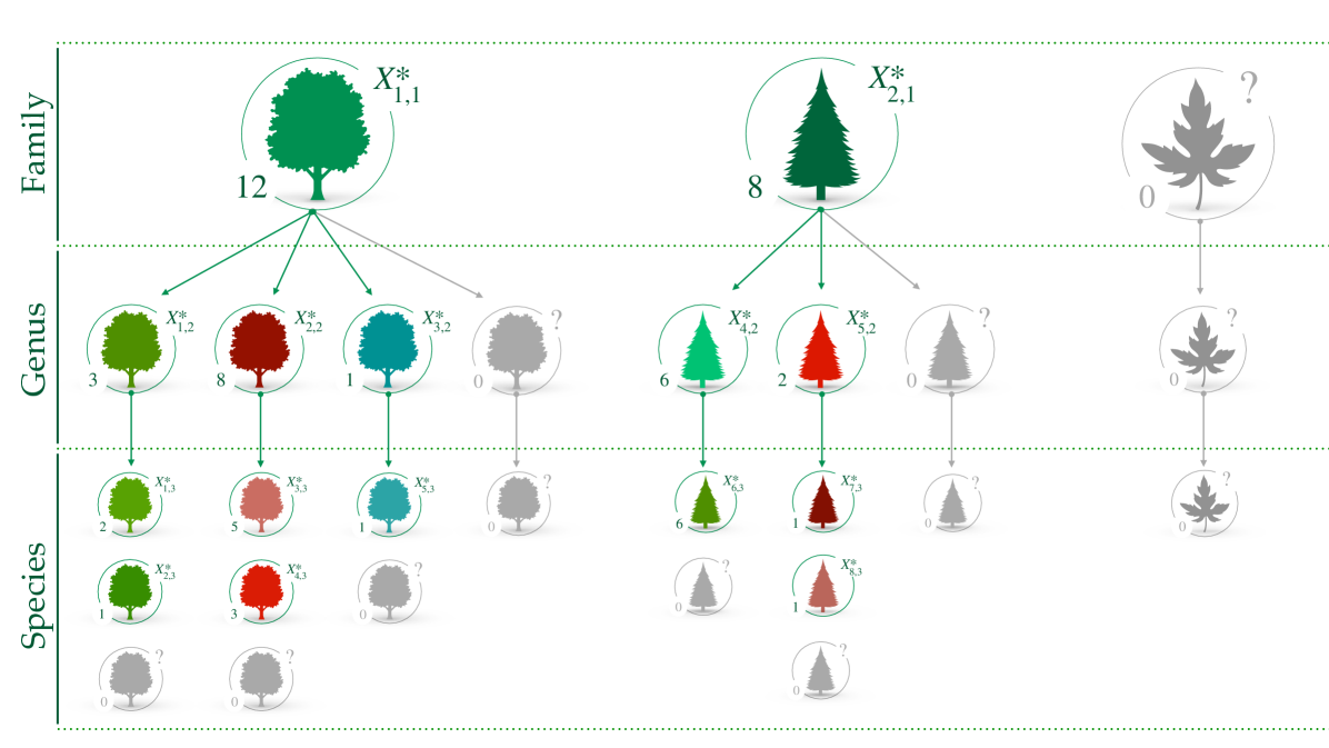
The model outlined in equations (13)-(15) admits a nested representation, depicted in Figure 2, which better clarifies the role of each . The observations can be sampled as follows:
for , and . The data of the first layer follows the same Gibbs-type mechanism that has been extensively described in Section 2. In the subsequent layers, say the th, the observations are grouped according to parent’s value . The data with the same parent are iid samples from , which, in turn, is distributed as a Gibbs-type process with weights . This representation leads to a predictive mechanism that extends (4). The discreteness of each implies that there will be ties in the realization of with positive probability. At the th layer, there will be distinct taxa with labels and frequencies , which may be grouped according to their parent. Let be the number of observations generated by the parent , let be the number of distinct labels generated by , and define the set , so that and . The predictive law is presented in the following proposition.
Proposition 3.
Proposition 3 expresses the learning mechanism in full generality, and it highlights the nested structure induced by taxonomic Gibbs-type priors. For specific choices of the predictive law can be specialized by replacing the ’s with their specific values. For instance, if and we get the following formula
which is a taxon-specific urn scheme. The diversity refers to observations whose parent is . The nested predictive mechanism described in Proposition 3 essentially states that (i) the data in the first layer of the taxonomy follow a Gibbs-type process; (ii) the data for the subsequent branches follow independent predictive mechanisms that are specific to the value of the parent level. As depicted in Figure 2, if a new taxon is observed at a certain layer of the taxonomy, it leads to the discovery of new values for all the children levels.
4.2 Estimation of conditional biodiversity
Compared to classical species sampling models, taxonomic Gibbs-type priors allow us to describe conditional biodiversities of specific branches of the taxonomy. The first layer is modeled as a classical Gibbs-type prior, with a single -diversity , a case that has been extensively discussed in Section 2. Conversely, at the generic th layer there are, potentially, infinitely many -diversities , one for each value of . So far, we have treated the diversities as deterministic, but in practice, they must be learned from the data, and this requires careful prior elicitation. A sample provides information only about the diversities associated to the observed taxa, for . Moreover, from the independence of random conditional distributions , the likelihood function of a taxonomic Gibbs-type model factorizes as follows
| (16) |
where . The likelihood function underlines that the data alone are not informative about the unobserved branches of the taxonomy, i.e., about whenever the taxon has not been observed in the sample.
We offer some suggestions on modeling the infinite collection of conditional diversities . A simple approach assumes that the ’s are iid samples from a layer-specific prior law , for any , independently over . This is computationally convenient because the posterior distributions of the conditional -diversities are independent due to the factorized likelihood in (16), and they can be inferred by applying the tools of Section 2 for each . However, the posterior law of for any unobserved taxon coincides with its prior distribution because there is no information in the likelihood. Hence, it is appealing to borrow information across conditional diversities belonging to the same layer through hierarchical modelling. For example, when we may specify , where each follows a hyperprior. Such a specification borrows strength among the diversities within the same layer , but not across. The factorized structure of (16) ensures that mcmc algorithms can be carried out separately for each layer. We will consider an example in Section 5.2. More sophisticated approaches may induce dependence across layers, for example, incorporating phylogenetic information, but we do not pursue this here.
Remark 4.
Marginal and conditional -diversities provide two different, but complementary, summaries of a complex phenomenon. Conditional diversities strongly depend on the chosen taxonomical structure. Potentially the models developed in this article can be used in concert with models characterizing variation in genetic sequences and morphology data for automatic taxonomic classification of samples, allowing for the discovery of new taxa, in a related manner to Zito et al. (2023).
5 The tree flora in the Amazonian Basin
5.1 The estimation of -diversity
We consider the comprehensive tree data set from the Amazon Basin and the Guiana Shield (Amazonia) provided by ter Steege et al. (2013), which is openly accessible online. This dataset integrates multiple sources and includes sampling plots well distributed among regions and forest types of the Amazon Basin, whose locations are shown in Figure 1(a). The immense size of the Amazon Basin has limited research on its tree communities at local and regional levels. Scientists still lack a complete understanding of the number of species in the Amazon, as well as their abundance and rarity (Hubbell et al., 2008; ter Steege et al., 2013), which leaves the world’s largest tropical carbon reserve mostly unknown to ecologists. The plots included a total of tree species, comprising genera and families, based on observations. In ter Steege et al. (2013), Fisher’s log-series model was applied to estimate the total number of species, generating approximately tree species. About of these species were classified as hyperdominant, which means they are so common that, collectively, they represent half of all trees in the Amazon. These estimates suggest that there may be over rare and poorly known species in the Amazon that could be at risk. We aim to provide a more refined statistical analysis of these data based on a Bayesian nonparametric analysis of the -diversity. In practice, our model-based approach allows us to: (i) check the validity of the underlying assumptions of the model; (ii) provide formal tools for uncertainty quantification even in the presence of model misspecification; (iii) tie together multiple aspects of the analysis within a unified model, making it clear and coherent.
The observations represent tree species and are assumed to be exchangeable under a Gibbs-type species sampling model. In particular, we will show that it is reasonable to assume , leading to the following hierarchical model:
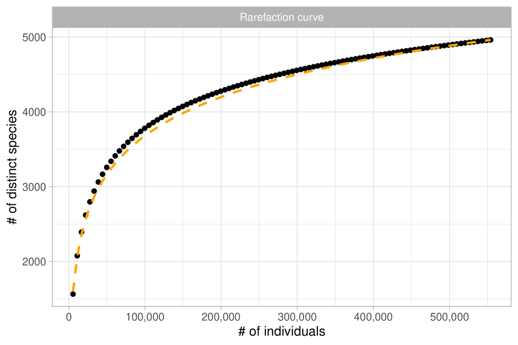
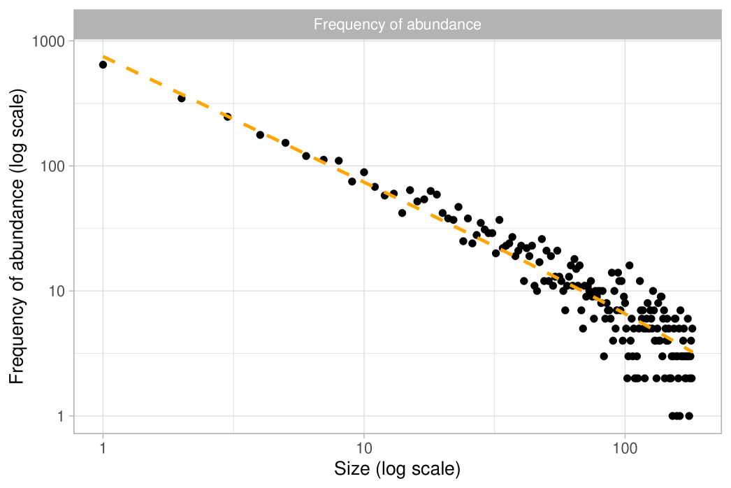
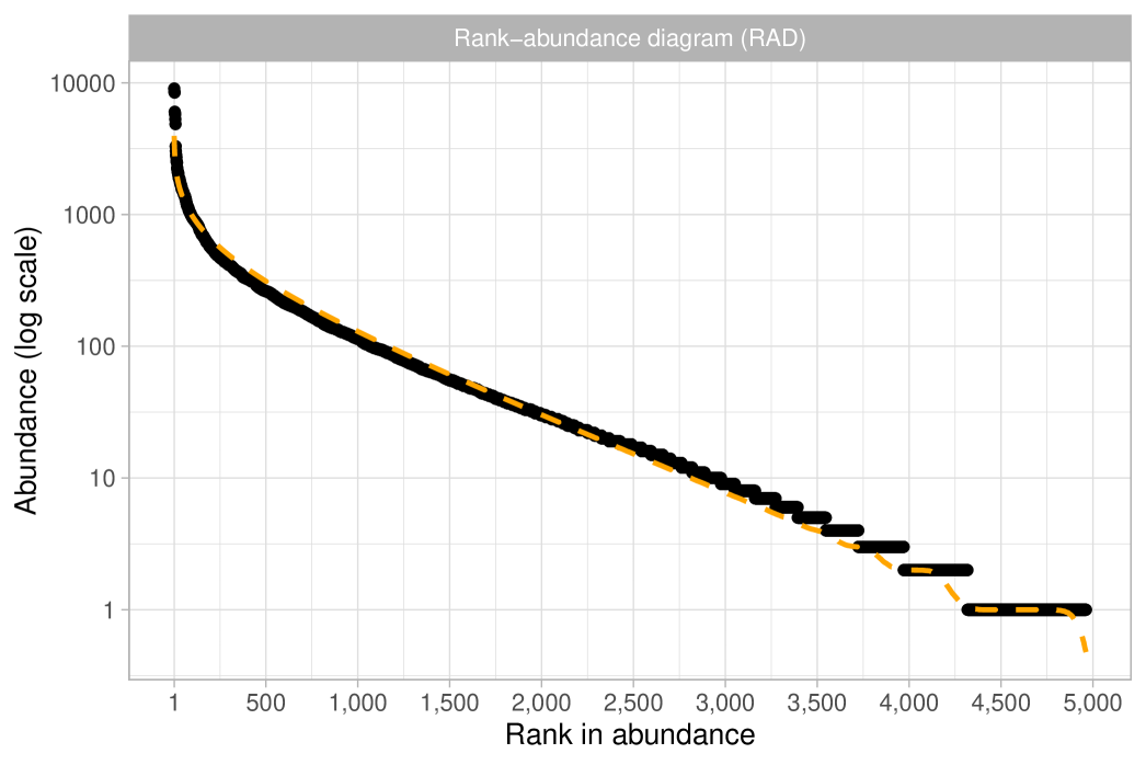
Recall that this specification is equivalent to Fisher’s log-series model. As a preliminary step, we obtain a maximum likelihood estimate for the fundamental biodiversity number of and a Fisher’s estimate of . The former was calculated using the BNPvegan R package (Zito et al., 2023), while the latter was obtained through the vegan R package (Oksanen et al., 2024). As previously mentioned, these two estimates are asymptotically equivalent and nearly indistinguishable for large . To assess the validity of the Dirichlet process specification we follow the guidelines outlined in Section 2.4 and we consider the quantities and . We then compare these expectations with their empirical counterparts, as displayed in Figure 3 (rarefaction) and Figure 4 (frequency of abundance). Both plots give similar conclusions: although the fit is not perfect, the predictions are remarkably close to the observed data. Indeed, the growth rate for the number of distinct species in Figure 3 looks roughly logarithmic, supporting the choice . At the same time, there are mild discrepancies between the data and the model predictions: the empirical rarefaction curve has a slightly higher curvature than the model fit. Moreover, Figure 4 shows that the Dirichlet process model slightly overestimates the number of singletons, and in particular, we get and . Finally, we show in Figure 5 the rank in abundance diagram (rad), which is the main graphical tool considered in ter Steege et al. (2013) to validate the adequacy of the Fisher’s log-series model. Once again, we conclude that the fit is quite good.
Despite its good predictive performance, the Dirichlet process is likely misspecified in this context. The data originates from multiple studies, each examining different regions and forests, which makes the exchangeability assumption for unlikely to hold. Supporting this concern, classical nonparametric and frequentist estimators such as those by Chao (1984), Chao and Lee (1992), and Chao and Bunge (2002) yield predictions–and associated confidence intervals–of between 5,000 and 6,000 for the total number of distinct species. These values were computed using the SPECIES R package (Wang, 2011). However, ter Steege et al. (2013) criticized these predictions, labeling them as “severe underestimations”, due to sharp disagreement with previous studies and expert assessments. This failure of standard nonparametric methods is not unusual in ecological studies (Brose et al., 2003), where assumptions often do not hold. Such estimators typically perform well in localized settings, but here we are considering the entire Amazon Basin. In contrast, the inherent “rigidity” of the Dirichlet process model enforces a logarithmic growth rate, which helps to avoid overfitting to the observed data, thus potentially mitigating the effects of misspecification.
With these considerations in mind, we proceed to conduct a full Bayesian analysis, accounting for potential model misspecification through the use of coarsened posteriors (Miller and Dunson, 2019). In practice, this is approximately achieved by raising the likelihood function to a factor , which effectively deflates the sample size and increases the uncertainty; taking recovers the standard posterior. For our analysis, the coarsened posterior distribution for becomes:
A natural prior choice is , the Stirling-gamma distribution of Zito et al. (2024) with parameters , where and . This prior interacts well with coarsened posteriors, remaining conjugate even after tempering the likelihood. Specifically, under a Stirling-gamma prior, the coarsened posterior is given by , resulting in:
Here, serves as the location of the prior distribution,while acts as a precision (Zito et al., 2024). In particular, we have , the prior estimate of the number of distinct species in a sample of size . In our analysis, we set and , implying , thus providing a non-informative prior centered on a plausible guess. Thanks to conjugacy, i.i.d. sampling from the coarsened posterior is straightforward through the algorithm of Zito et al. (2024).
| Equivalent sample size () | 1% | 25% | 50% | Mean | 75% | 99% | |
|---|---|---|---|---|---|---|---|
| Fundamental biodiversity number | |||||||
| 1 | 553,949 | 725 | 743 | 751 | 751 | 759 | 779 |
| 0.25 | 138,487 | 699 | 736 | 751 | 751 | 767 | 806 |
| 0.1 | 55,395 | 669 | 726 | 751 | 751 | 776 | 839 |
| 0.01 | 5,539 | 514 | 673 | 747 | 753 | 827 | 1,048 |
| 0.001 | 554 | 208 | 517 | 713 | 766 | 956 | 1,792 |
| Total number of tree species | |||||||
| 1 | 553,949 | 14,378 | 14,841 | 15,065 | 15,051 | 15,267 | 15,678 |
| 0.25 | 138,487 | 14,139 | 14,777 | 15,052 | 15,052 | 15,327 | 15,976 |
| 0.1 | 55,395 | 13,814 | 14,675 | 15,045 | 15,054 | 15,422 | 16,371 |
| 0.01 | 5,539 | 11,824 | 13,981 | 14,990 | 15,077 | 16,077 | 19,097 |
| 0.001 | 554 | 7752 | 11,906 | 14,533 | 15,246 | 17,800 | 29,058 |
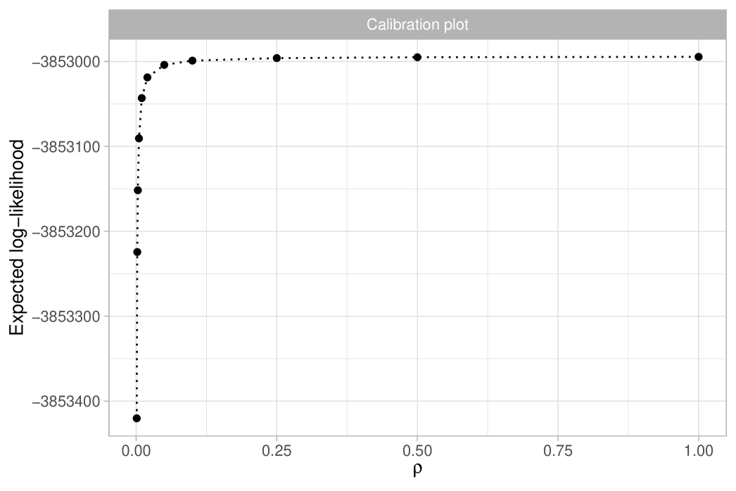
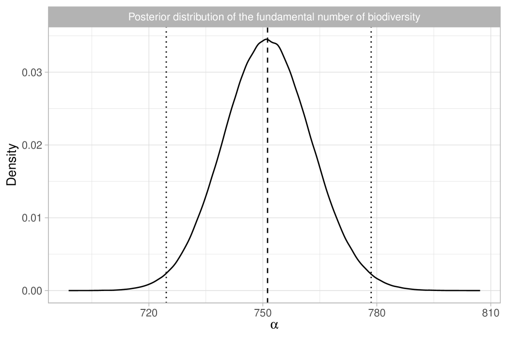
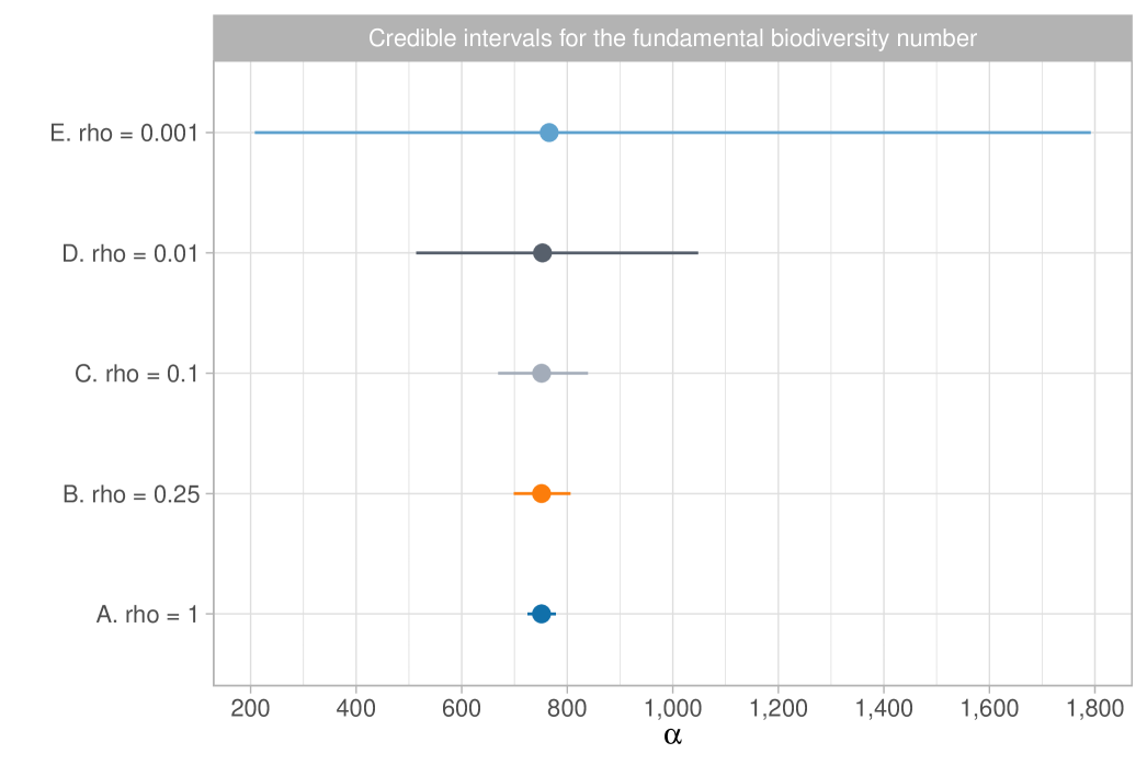
We report the results in Table 1, which shows posterior means and quantiles for under various choices of the tempering parameter . Choosing is challenging, as it requires accurately quantifying the degree of misspecification. Table 1 also includes the equivalent sample size ; we note that, except for the extreme case of , the posterior means and medians remain stable, approximately matching the maximum likelihood estimate of . The value of has a substantial impact on posterior variability, with smaller values representing conservative choices by leading to greater uncertainty. Assuming the model is correctly specified, the credible interval for is . However, with a moderate level of coarsening, say , the 98% credible interval broadens to . Notably, the independent estimate for the Amazon Basin from Hubbell et al. (2008) lies within both intervals. We provide graphical support for in the Supplementary Material, using an informal elbow rule to identify the smallest that does not lead to strong incompatibilities with the observed data, as measured by the likelihood function (Miller and Dunson, 2019). Figure 1(b) displays the coarsened posterior for with . The posterior distribution of , the fundamental biodiversity number, encapsulates various aspects of the data. For example, for large , the expected number of singletons is , so the interval serves also as an estimate for the number of singletons. This also supports the choice , given that the observed number of singletons is , which lies well outside the credible interval of the standard posterior. As detailed in Section 2.3, other biodiversity measures can be derived from the posterior distribution of . For instance, the posterior mean for the Simpson diversity, , is , while the posterior mean for Shannon diversity is .
The most interesting quantity we wish to estimate is arguably the total number of tree species in the Amazon Basin. In ter Steege et al. (2013), this is estimated using Fisher’s log series model in a relatively ad-hoc manner, by extrapolating the rad shown in Figure 5 to obtain approximately 15,000 to 16,000 tree species, depending on the extrapolation method used. Here, we present a more mathematically rigorous approach that also properly quantifies the associated uncertainty. Let us first recall that in the Dirichlet process model, diverges as grows. However, this should not be viewed as a shortcoming of the model. The population size , representing the total number of trees in the Amazon Basin, is finite, implying that the total number of tree species is . Furthermore, ter Steege et al. (2013) provides a reliable estimate of the population size, , based on observed tree density. To be robust against potential errors in this estimate, we specify a prior for centered on by letting . This prior choice is roughly consistent with the standard errors for given in ter Steege et al. (2013). Note we cannot learn based on the publicly available data, so we rely on external information for this inferential step. In summary, the coarsened posterior distribution for the total number of tree species can be obtained through the following sampling steps:
In Section 2, we described general formulas for the law , which could, in principle, be applied here. Additionally, note that the posterior expectation of is . For simplicity and computational efficiency, we rely on a well-known, highly accurate Poisson approximation valid for large values of :
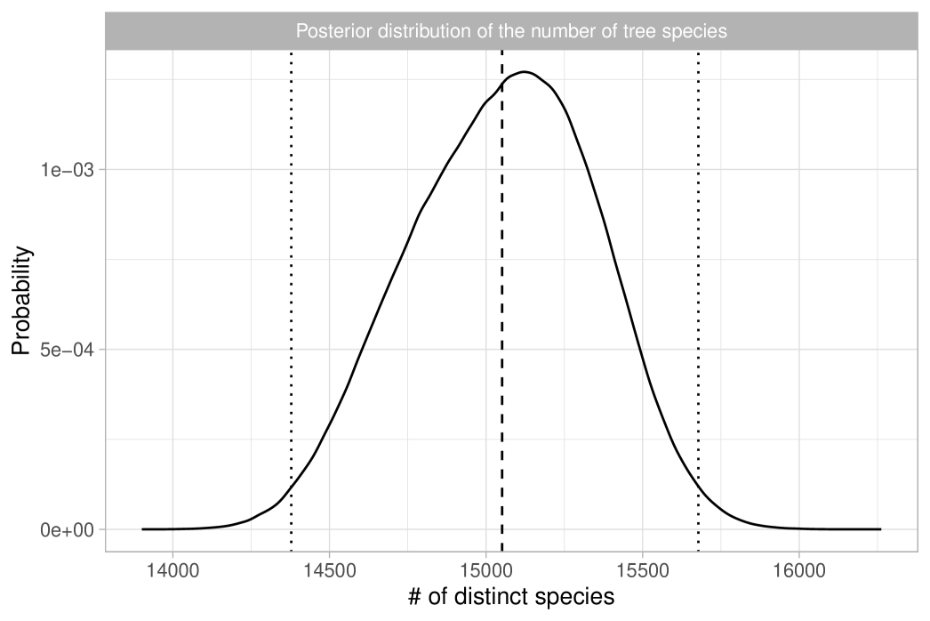
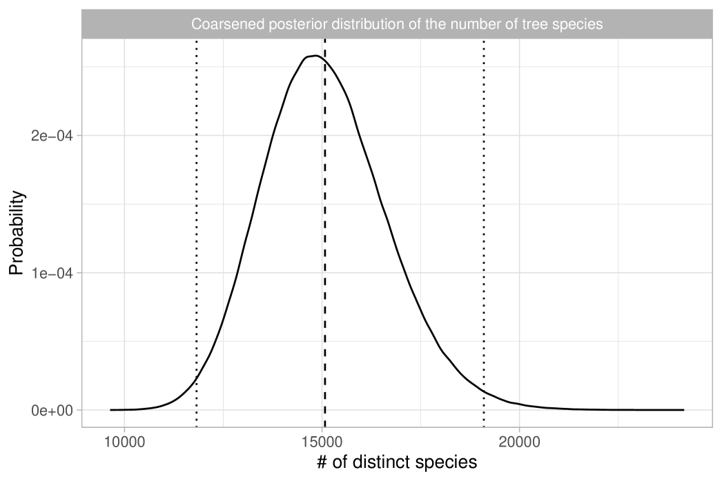
where means “approximately distributed as”, recalling that, given the data, we have . This approximation can be rigorously justified in terms of total variation convergence, which holds for large values of ; see Proposition 4.8 in Ghosal and Van der Vaart (2017). We report the results in Table 1, which shows posterior means and quantiles for under various choices of the tempering parameter. Figure 6 displays the coarsened posterior of with . Our analysis suggests that the Bayesian estimate for the total number of tree species is approximately 15,000, consistent with the main finding of ter Steege et al. (2013). Additionally, we estimate a 98% credible interval for this total to be between 11,800 and 19,100 when . Notably, due to the logarithmic growth rate, the uncertainty in the posterior distribution of is primarily influenced by the variability in , rather than potential misspecifications of the population size .
5.2 Taxonomic -diversity
We now describe a more nuanced analysis of the Amazon tree dataset that incorporates the taxonomic structure of the data. This analysis uses the taxonomic Gibbs-type priors introduced in Section 4 with , where the exchangeable observations are triplets, denoted , whose elements represent the family, genus, and species of the th tree, respectively. The last element of each triplet, , corresponds to the previously analyzed tree species. We let the family labels be iid samples from , where for . Moreover, for the genera and species, we assume the observations as generated as follows
We specify different priors for the second and third layers of the taxonomy. Denoting by and , we assume
In other words, we assume a logarithmic growth rate for genera within families and a faster polynomial growth rate for species within each genus, induced by the Aldous-Pitman model. This taxonomic approach allows us to compare the genus-level biodiversity within each family, denoted by , as well as the species-level biodiversity within each genus, denoted by . To get Bayesian estimates for and we need to specify priors and . In the former case, we let , with , , , a fairly informative prior according to which we expect, a priori and on average, 3 distinct genera for each family, in a hypothetical sample from the same family of size . On the other hand, we assume a hierarchical prior for , to borrow strength across species-level biodiversities, which is needed due to the sparsity of the data. Specifically, we let
where we set and .
We ran an mcmc algorithm for 10,000 iterations, discarding the first 1,000 as burn-in; the computational details are provided in the Supplementary Material. The sampling algorithm is particularly straightforward due to the factorized likelihood (16). This, combined with suitable priors and , results in separate blocks of the model that can be estimated independently. The posterior distribution for the most relevant part of the model–the one describing species-within-genera biodiversity–has been coarsened with to address potential misspecification. As before, this choice of coarsening is supported by an informal elbow rule.
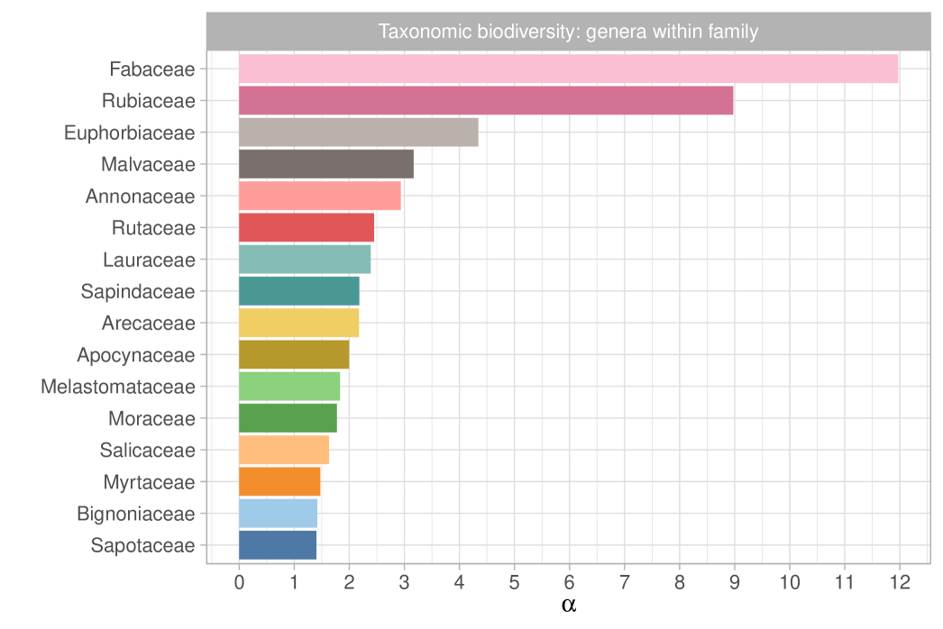
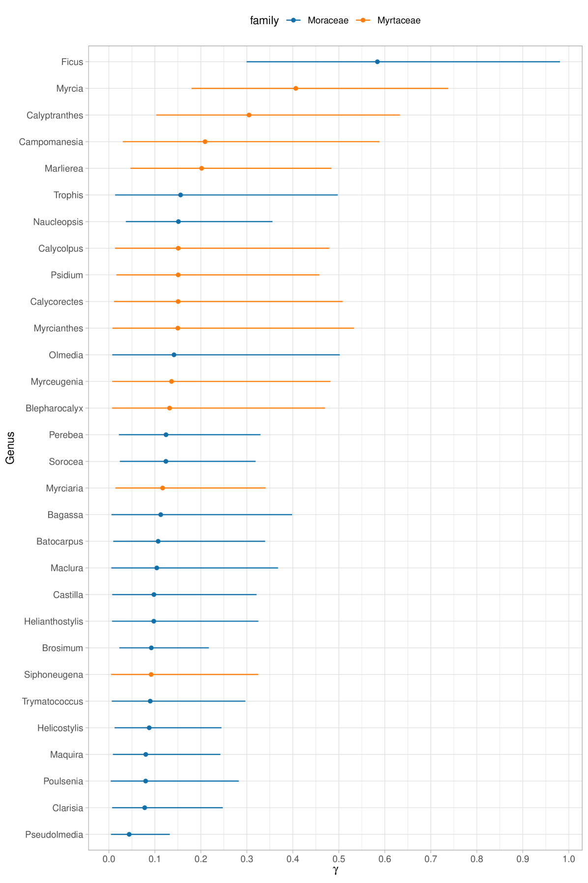
We report in Figure 7 the posterior expectations for selected families. Specifically, we show the 16 most diverse of 115 families, as measured by the fundamental biodiversity numbers . These values represent family-specific biodiversity that accounts for the variety of genera within the same taxonomic branch. However, it is important to note that does not reflect the number of species within each genus. The most biodiverse family is Fabaceae, which is expected, since it is also the most abundant and rich family in the dataset. Furthermore, as observed in ter Steege et al. (2013), Rubiaceae–the second most diverse family according to –has relatively few hyperdominant species, which aligns with its high diversity number. Moreover, in Figure 8, we plot the posterior distributions of select genus-specific biodiversities for all genera in two randomly chosen families, Moraceae and Myrtaceae. As the plot suggests, with few exceptions, there is substantial uncertainty in each , though this is partially reduced by borrowing strength across genera. In particular, in our hierarchical model, the estimated average biodiversity is with a standard deviation of . Two genera that stand out from the average behavior are Ficus and Pseudolmedia. The former ranks among the most diverse genera of trees, as evidenced by the extensive list of species documented in Plants of the World Online (https://powo.science.kew.org); see Baker et al. (2022). To date, there are almost a thousand accepted species of Ficus spread across Amazonia and other regions of the world. In contrast, Pseudolmedia has only 11 known species globally (four of them observed in our dataset), all situated in the Amazon basin and adjacent areas; some of these species may be at risk of extinction.
6 Discussion
In this paper, we discuss what we believe to be one of the most natural definitions of biodiversity from a Bayesian perspective, unifying accumulation curves, and most existing biodiversity measures under a model-based approach. Mathematically, this approach takes advantage of Gibbs-type priors as defined in Gnedin and Pitman (2005), although most of the inferential results crucial for species discovery were developed in a subsequent paper by Lijoi et al. (2007a). This theory has significant connections with ideas developed over the years, particularly by Fisher et al. (1943) and Hubbell (2001). A key natural question is understanding generalizations to different sampling mechanisms, such as those where only species presence is recorded (i.e. incidence data). This has recently been addressed in Ghilotti et al. (2024), which introduced a broad class of models sharing structural properties with Gibbs-type priors and leads to a natural notion of biodiversity for incidence data.
We also envision several promising research directions. First, we observe that a systematic comparison of priors for , representing species richness in a Dirichlet-multinomial model, is currently lacking. This is a straightforward next step that could be effectively explored with moderate effort, at least from an empirical standpoint. A second and more complex issue involves the inclusion of covariates. Estimating localized biodiversity metrics for specific regions or tracking biodiversity changes over time is both more interesting and realistic than estimating a single biodiversity number. However, directly applying covariate-dependent Dirichlet processes (e.g., Quintana et al., 2022) appears unsuitable and requires careful modifications. The work of Zito et al. (2023) goes in that direction by incorporating DNA sequencing into the model, but it does not provide synthetic measures of biodiversity. A third relevant issue refers to a clear definition of the so-called “beta” diversity, namely the heterogeneity of species across different sampling regions. Recently, there have been sensible developments in models that can account for shared species, most notably the hierarchical constructions described in Camerlenghi et al. (2017), Camerlenghi et al. (2019). However, some computational challenges remain open, as well as a precise notion of “beta” diversity which should be as clear and unifying as the -diversity described in this paper.
Acknowledgments
Tommaso Rigon acknowledges support of MUR - Prin 2022 - Grant no. 2022CLTYP4, funded by the European Union - Next Generation EU. This work was partially supported by the European Research Council under the European Union’s Horizon 2020 research and innovation programme (grant agreement No 856506).
References
- Aldous and Pitman (1998) Aldous, D. and J. Pitman (1998). The standard additive coalescent. Ann. Probab. 26(4), 1703–1726.
- Baker et al. (2022) Baker, W. J., P. Bailey, V. Barber, A. Barker, S. Bellot, D. Bishop, L. R. Botigué, G. Brewer, T. Carruthers, J. J. Clarkson, J. Cook, R. S. Cowan, S. Dodsworth, N. Epitawalage, E. Françoso, B. Gallego, M. G. Johnson, J. T. Kim, K. Leempoel, O. Maurin, C. McGinnie, L. Pokorny, S. Roy, M. Stone, E. Toledo, N. J. Wickett, A. R. Zuntini, W. L. Eiserhardt, P. J. Kersey, I. J. Leitch, and F. Forest (2022). A Comprehensive Phylogenomic Platform for Exploring the Angiosperm Tree of Life. Systematic Biology 71(2), 301–319.
- Blackwell and MacQueen (1973) Blackwell, D. and J. B. MacQueen (1973). Ferguson distributions via Pólya urn schemes. Ann. Statist. 1(2), 353–355.
- Brose et al. (2003) Brose, U., N. D. Martinez, and R. J. Williams (2003). Estimating species richness: Sensitivity to sample coverage and insensitivity to spatial patterns. Ecology 84(9), 2364–2377.
- Bunge and Fitzpatrick (1993) Bunge, J. and M. Fitzpatrick (1993). Estimating the number of species: a review. J. Am. Statist. Ass. 88(421), 364–373.
- Camerlenghi et al. (2019) Camerlenghi, F., A. Lijoi, P. Orbanz, and I. Prünster (2019). Distribution theory for hierarchical processes. Ann. Statist. 47(1), 67–92.
- Camerlenghi et al. (2017) Camerlenghi, F., A. Lijoi, and I. Prünster (2017). Bayesian prediction with multiple-samples information. J. Multiv. Anal. 156, 18–28.
- Ceballos et al. (2015) Ceballos, G., P. R. Ehrlich, A. D. Barnosky, A. García, R. M. Pringle, and T. M. Palmer (2015). Accelerated modern human-induced species losses: Entering the sixth mass extinction. Science Advances 1(5), 9–13.
- Chao (1984) Chao, A. (1984). Nonparametric estimation of the number of classes in a population. Scand. J. Statist. 11(4), 265–270.
- Chao and Bunge (2002) Chao, A. and J. Bunge (2002). Estimating the number of species in a stochastic abundance model. Biometrics 58(3), 531–539.
- Chao and Lee (1992) Chao, A. and S. M. Lee (1992). Estimating the number of classes via sample coverage. J. Am. Statist. Ass. 87(417), 210–217.
- Charalambides (2002) Charalambides, C. A. (2002). Enumerative combinatorics. Springer.
- Chisholm and Burgman (2004) Chisholm, R. A. and M. A. Burgman (2004). The unified neutral theory of biodiversity and biogeography: comment. Ecology 85(11), 3172–3174.
- Colwell (2009) Colwell, R. K. (2009). Biodiversity: concepts, patterns, and measurement, pp. 257–263. Princeton University Press.
- Colwell et al. (2012) Colwell, R. K., A. Chao, N. J. Gotelli, S.-Y. Lin, C. X. Mao, R. L. Chazdon, and J. T. Longino (2012). Models and estimators linking individual-based and sample-based rarefaction, extrapolation and comparison of assemblages. J. Plant Ecol. 5(1), 3–21.
- De Blasi et al. (2015) De Blasi, P., S. Favaro, A. Lijoi, R. H. Mena, I. Prunster, and M. Ruggiero (2015). Are Gibbs-type priors the most natural generalization of the Dirichlet process? IEEE Trans. Pattern Anal. Mach. Intell. 37(2), 212–229.
- De Blasi et al. (2013) De Blasi, P., A. Lijoi, and I. Prünster (2013). An asymptotic analysis of a class of discrete nonparametric priors. Statist. Sin. 23(3), 1299–1321.
- de Finetti (1937) de Finetti, B. (1937). La prévision: ses lois logiques, ses sources subjectives. Annales de l’institut Henri Poincaré 7, 1–68.
- Devroye (1986) Devroye, L. (1986). Non-Uniform Random Variate Generation. Springer.
- Escobar and West (1995) Escobar, M. D. and M. West (1995). Bayesian density estimation and inference using mixtures. J. Am. Statist. Ass. 90(430), 577–588.
- Favaro et al. (2009) Favaro, S., A. Lijoi, R. H. Mena, and I. Prünster (2009). Bayesian non-parametric inference for species variety with a two-parameter Poisson-Dirichlet process prior. J. R. Statist. Soc. B 71(5), 993–1008.
- Favaro et al. (2012) Favaro, S., A. Lijoi, and I. Prünster (2012). Asymptotics for a Bayesian nonparametric estimator of species variety. Bernoulli 18(4), 1267–1283.
- Favaro et al. (2013) Favaro, S., A. Lijoi, and I. Prünster (2013). Conditional formulae for Gibbs-type exchangeable random partitions. Ann. Appl. Probab. 23(5), 1721–1754.
- Favaro et al. (2015) Favaro, S., M. Lomeli, and Y. W. Teh (2015). On a class of sigma-stable Poisson–Kingman models and an effective marginalized sampler. Statist. Comp. 25(1), 67–78.
- Favaro et al. (2021) Favaro, S., F. Panero, and T. Rigon (2021). Bayesian nonparametric disclosure risk assessment. Electron. J. Statist. 15(2), 5626–5651.
- Ferguson (1973) Ferguson, T. S. (1973). A Bayesian analysis of some nonparametric problems. Ann. Statist. 1(2), 209–230.
- Fisher et al. (1943) Fisher, R. A., A. S. Corbet, and C. B. Williams (1943). The relation between the number of species and the number of individuals in a random sample of an animal population. J. Anim. Ecol. 12(1), 42–58.
- Ghilotti et al. (2024) Ghilotti, L., F. Camerlenghi, and T. Rigon (2024). Bayesian analysis of product feature allocation models. arXiv:2408.15806.
- Ghosal and Van der Vaart (2017) Ghosal, S. and A. Van der Vaart (2017). Fundamentals of nonparametric Bayesian inference. Cambridge University Press.
- Gnedin (2010) Gnedin, A. (2010). Species sampling model with finitely many types. Electron. Comm. Prob. 15, 79–88.
- Gnedin and Pitman (2005) Gnedin, A. and J. Pitman (2005). Exchangeable Gibbs partitions and Stirling triangles. Zapiski Nauchnykh Seminarov, POMI 325, 83–102.
- Good (1953) Good, I. J. (1953). The population frequencies of species and the estimation of population parameters. Biometrika 40(3-4), 237–264.
- Good and Toulmin (1956) Good, I. J. and G. H. Toulmin (1956). The number of new species, and the increase in population coverage, when a sample is increased. Biometrika 43(1-2), 45–63.
- Gotelli and Colwell (2001) Gotelli, N. J. and R. K. Colwell (2001). Quantifying biodiversity: procedures and pitfalls in the measurement and comparison of species richness. Ecol. Lett. 4, 379–391.
- Hjort et al. (2010) Hjort, N. L., C. Holmes, P. Müller, and S. G. Walker (2010). Bayesian nonparametrics, Volume 28. Cambridge University Press.
- Hubbell (2001) Hubbell, S. P. (2001). The Unified Neutral Theory of Biodiversity and Biogeography. Princeton University Press.
- Hubbell et al. (2008) Hubbell, S. P., F. He, R. Condit, L. Borda-de Água, J. Kellner, and H. Ter Steege (2008). How many tree species are there in the Amazon and how many of them will go extinct? Proceedings of the National Academy of Sciences of the United States of America 105, 11498–11504.
- Kingman (1975) Kingman, J. F. (1975). Random discrete distributions. J. R. Statist. Soc. B 37(1), 1–15.
- Korwar and Hollander (1973) Korwar, R. M. and M. Hollander (1973). Contributions to the theory of Dirichlet processes. Ann. Probab. 1(4), 705–711.
- Lebedev (1965) Lebedev, N. N. (1965). Special functions and their applications. Prentice-Hall, Inc.
- Legramanti et al. (2022) Legramanti, S., T. Rigon, D. Durante, and D. B. Dunson (2022). Extended stochastic block models with application to criminal networks. Ann. Appl. Stat. 16(4), 2369–2395.
- Lijoi et al. (2005) Lijoi, A., R. H. Mena, and I. Prünster (2005). Hierarchical mixture modeling with normalized inverse-Gaussian priors. J. Am. Statist. Ass. 100(472), 1278–1291.
- Lijoi et al. (2007a) Lijoi, A., R. H. Mena, and I. Prünster (2007a). Bayesian nonparametric estimation of the probability of discovering new species. Biometrika 94(4), 769–786.
- Lijoi et al. (2007b) Lijoi, A., R. H. Mena, and I. Prünster (2007b). Controlling the reinforcement in Bayesian non-parametric mixture models. J. R. Statist. Soc. B 69(4), 715–740.
- Lijoi et al. (2008a) Lijoi, A., I. Prünster, and S. G. Walker (2008a). Bayesian nonparametric estimators derived from conditional Gibbs structures. Ann. Appl. Probab. 18(4), 1519–1547.
- Lijoi et al. (2008b) Lijoi, A., I. Prünster, and S. G. Walker (2008b). Investigating nonparametric priors with Gibbs structure. Statist. Sin. 18(4), 1653–1668.
- Magurran and McGill (2011) Magurran, A. E. and B. J. McGill (2011). Biological Diversity: frontiers in measurement and assessment. Oxford Biology.
- McCullagh (2016) McCullagh, P. (2016). Two early contributions to the Ewens saga. Statist. Sci. 31(1), 23–26.
- McGill (2003) McGill, B. J. (2003). A test of the unified neutral theory of biodiversity. Nature 422(6934), 881–885.
- Miller and Dunson (2019) Miller, J. W. and D. B. Dunson (2019). Robust Bayesian inference via coarsening. J. Am. Statist. Ass. 114(527), 1113–1125.
- Miller and Harrison (2018) Miller, J. W. and M. T. Harrison (2018). Mixture models with a prior on the number of components. J. Am. Statist. Ass. 113(521), 340–356.
- Oksanen et al. (2024) Oksanen, J., G. L. Simpson, F. G. Blanchet, R. Kindt, P. Legendre, P. R. Minchin, R. O’Hara, P. Solymos, M. H. H. Stevens, E. Szoecs, H. Wagner, M. Barbour, M. Bedward, B. Bolker, D. Borcard, G. Carvalho, M. Chirico, M. De Caceres, S. Durand, H. B. A. Evangelista, R. FitzJohn, M. Friendly, B. Furneaux, G. Hannigan, M. O. Hill, L. Lahti, D. McGlinn, M.-H. Ouellette, E. Ribeiro Cunha, T. Smith, A. Stier, C. J. Ter Braak, and J. Weedon (2024). vegan: Community Ecology Package. R package version 2.6-8.
- Perman et al. (1992) Perman, M., J. Pitman, and M. Yor (1992). Size-biased sampling of Poisson point processes and excursions. Probability Theory and Related Fields 92(1), 21–39.
- Pitman (1996) Pitman, J. (1996). Some developments of the Blackwell-MacQueen urn scheme. In Statistics, probability and game theory, Volume 30 of IMS Lecture Notes Monogr. Ser., pp. 245–267. Inst. Math. Statist., Hayward, CA.
- Pitman (2003) Pitman, J. (2003). Poisson-Kingman partitions. Lecture Notes-Monograph Series 40, 1–34.
- Pitman (2006) Pitman, J. (2006). Combinatorial stochastic processes: Ecole d’eté de probabilités de saint-flour xxxii-2002. Springer.
- Pitman and Yor (1997) Pitman, J. and M. Yor (1997). The two-parameter Poisson-Dirichlet distribution derived from a stable subordinator. Ann. Probab. 25(2), 855–900.
- Quintana et al. (2022) Quintana, F. A., P. Müller, A. Jara, and S. N. MacEachern (2022). The Dependent Dirichlet Process and Related Models. Statist. Sc. 37(1), 24–41.
- Ricklefs (2006) Ricklefs, R. E. (2006). The unified neutral theory of biodiversity: do the numbers add up? Ecology 87(6), 1424–1431.
- Rigon et al. (2025) Rigon, T., S. Petrone, and B. Scarpa (2025). Enriched Pitman-Yor processes. Scand. J. Statist..
- Sethuraman (1994) Sethuraman, J. (1994). A constructive definition of Dirichlet priors. Statist. Sin. 4(2), 639–650.
- Smith and Grassle (1977) Smith, W. and J. F. Grassle (1977). Sampling properties of a family of diversity measures. Biometrics 33(2), 283–292.
- Sun et al. (2023) Sun, J., M. Kong, and S. Pal (2023). The Modified-Half-Normal distribution: Properties and an efficient sampling scheme. Commun. Statist. Th. Meth. 52(5), 1591–1613.
- ter Steege et al. (2013) ter Steege, H. et al. (2013). Hyperdominance in the amazonian tree flora. Science 342(6156), 1243092.
- Thisted and Efron (1987) Thisted, R. and B. Efron (1987). Did Shakespeare write a newly-discovered poem? Biometrika 74(3), 445–455.
- Wade et al. (2011) Wade, S., S. Mongelluzzo, S. Petrone, et al. (2011). An enriched conjugate prior for Bayesian nonparametric inference. Bayesian Analysis 6(3), 359–385.
- Wang (2011) Wang, J. P. (2011). SPECIES: An R package for species richness estimation. J. Statist. Soft. 40(9), 1–15.
- Zito et al. (2023) Zito, A., T. Rigon, and D. B. Dunson (2023). Inferring taxonomic placement from DNA barcoding allowing discovery of new taxa. Meth. Ecol. Evol. 14, 529–542.
- Zito et al. (2024) Zito, A., T. Rigon, and D. B. Dunson (2024). Bayesian nonparametric modeling of latent partitions via Stirling-gamma priors. Bayesian Analysis (forthcoming).
- Zito et al. (2023) Zito, A., T. Rigon, O. Ovaskainen, and D. B. Dunson (2023). Bayesian modeling of sequential discoveries. J. Am. Statist. Ass. 188(544), 2521–2532.
Appendix A Proofs
A.1 Rarefaction and extrapolation curve of a Dirichlet-multinomial model
We present here the proof of the results in Example 4, concerning the expectations and in the Dirichlet multinomial model. To begin, let us recall that the process is defined as , where . The a priori expected value of the number of distinct values is well known (e.g. Pitman, 2006, Chap. 3), but we provide here a simple and alternative proof that does not require combinatorial calculus. Specifically, we have:
where the quantity is the probability of observing the th species at least once in a sample of size (Smith and Grassle, 1977) given the vector of probabilities . Hence:
where the last step follows because are iid beta random variables. In fact and from well-known properties of the beta distribution the result follows
This proof technique can be extended to the posteriori expectation . In fact, the posterior distribution of is conjugate, that is
where are the labeled frequencies of the species . Note that we could have , and the number of non-zero entries, that is, the number of observed species, is . Without loss of generality, we assume the non-zero abundances correspond to the first values, so that for and for . Reasoning as before, we obtain
where each for is the probability of sampling the th unobserved species at least once in an additional sample of size , given the vector of probabilities and the data . A posteriori, the random variables are still iid beta distributed and in particular leading to
Interestingly, this corresponds to the estimator of a Pitman–Yor process with a negative discount parameter; see equation (6) in Favaro et al. (2009). We also note that this result could be alternatively obtained, with some effort, specializing the general theorems of Lijoi et al. (2007a). A further proof strategy based on combinatorial calculus is discussed in Appendix A.1 and A.2 in Favaro et al. (2009).
A.2 Proof of Theorem 1
First of all, the quantity is a sufficient statistic for the diversity by direct inspection of the likelihood function, that is, the eppf. In fact, the diversity only appears in the terms which solely depend on and and not the abundances. From Proposition 2, we know that
that is, . Let , and and note that and , therefore . The proof follows from a very simple argument:
In other words, we have shown that . By a continuity argument, the sequences
also converge to almost surely as . We now clarify that the distribution of the random variable is indeed the posterior law of the parameters , , and . Let us first consider the three building blocks of Gibbs-type priors, namely when is a positive constant. The above result implies the convergence of the Laplace functionals, that is, for any ,
In a general Gibbs-type prior, converges to a random variable whose distribution is the posterior law of the diversity. In fact, as an application of the tower rule,
which concludes the proof.
A.2.1 Alternative proof of Theorem 1 for
We describe an alternative proof of Theorem 1, expressed in terms of weak convergence, which applies when . This proof technique is more direct, relying on calculus and combinatorics. In contrast, the previous proof is more abstract and depends on Proposition 2.
Let us consider the Dirichlet process case with parameter . We begin by studying the a priori asymptotic behavior of , a result that was established by Korwar and Hollander (1973). By definition, the Laplace transform of this scaled random variable is
The third equality follows by definition of signless Stirling numbers of the first kind. Now, let and note that . Thus
The second step follows by applying Stirling’s asymptotic formula for the Gamma function. Moreover, note that therefore
whereas
Summing up, we have shown that , which means that . The proof for the conditional case law follows from similar steps. Note that has the same asymptotic behavior as , since . Moreover, its Laplace transform is
The first step follows from the combinatorial identity established in Lijoi et al. (2007a). In the second step, we recognized that is an alternative representation of the signless non-central Stirling numbers of the first kind; see equation (8.60) in Charalambides (2002). The third simplification follows by definition of . Taking the limit, we obtain
The last step follows from analogous calculations done for the a priori case. This concludes the proof, as the case of general Gibbs-type prior with random and follows as an application of the tower rule, as before.
A.3 Aldous-Pitman data augmentation
In this Section we provide further details the discussion about the data augmentation for the Aldous-Pitman model described in Section 3. Let us begin by recalling the main result, that is the augmented likelihood
Integrating with respect to gives the eppf of an Aldous-Pitman model with weights in equation (10), because
From the augmented representation we immediately obtain, through direct inspection of the joint law, the full conditional distributions for and . In particular:
Moreover, let us recall the predictive distribution is
Substituting and with their integral representation, we obtain
and
Note that this predictive scheme still does not provide a manageable sampling algorithm for because the expectations and are not easily available. However, one can resort to Algorithm 1, which is based on the following additional data augmentation. Let us define a binary random variable such that iff and otherwise. Moreover, let be a positive random variable such that the joint law of and is:
and
Then, the sampling strategy is as follows: sample from its marginal distribution and then . Both distributions are easy to sample from and their laws are described in Algorithm 1. Once it has been determined whether the observation is either new or old, the remaining part of the sampling algorithm is trivial.
A.4 Proof of Proposition 3
The proof of this proposition follows by repeatedly applying the argument discussed in Rigon et al. (2025) for the enriched Pitman-Yor process, corresponding to the case where and the involved random measures are either Pitman–Yor processes or Dirichlet processes.
A.5 Details of the Gibbs sampling algorithm of Section 5.2
The augmented and coarsened likelihood of the model Section 5.2 is the following
where represents the collection of latent variables. Note that the likelihood function factorizes, allowing inference to be performed independently for each layer of the model. For layer 2, inference proceeds separately for each as described in Section 5.1, given that the priors for the diversities are independently distributed according to the Stirling-gamma distribution. On the other hand, a Gibbs-sampling algorithm is required for layer 3, alternating between these steps
-
1.
For sample independently from the (coarsened) full conditionals of the diveristies .
-
2.
For sample independently from the (coarsened) full conditionals of whose densities are . Exact sampling from this distribution is feasible using the algorithm described in Sun et al. (2023), or alternatively, through the ratio-of-uniform acceptance-rejection algorithm.
-
3.
Sample the hyperparameters from their full conditional distribution. This step is equivalent to sampling the posterior distribution of the parameters under the assumption that the data are i.i.d. Gamma distributed and the log-prior follows a multivariate Gaussian distribution. A standard Metropolis step is employed, using a carefully tuned Gaussian proposal distribution to ensure good mixing.
Appendix B Additional plots for the application in Section 5.1
Additional plot for the application discussed in Section 5.1. Simulated values are based on Monte Carlo replicates using the Stirling-gamma sampling algorithm of Zito et al. (2024) combined with a Poisson approximation for , as discussed in the main text.