A bound on partitioning clusters
Mathematics Subject Classifications: 11B30)
Abstract
Let be a finite collection of sets (or “clusters”). We consider the problem of counting the number of ways a cluster can be partitioned into two disjoint clusters , thus is the disjoint union of and ; this problem arises in the run time analysis of the ASTRAL algorithm in phylogenetic reconstruction. We obtain the bound
where denotes the cardinality of , and , so that . Furthermore, the exponent cannot be replaced by any larger quantity. This improves upon the trivial bound of . The argument relies on establishing a one-dimensional convolution inequality that can be established by elementary calculus combined with some numerical verification.
In a similar vein, we show that for any subset of a discrete cube , the additive energy of (the number of quadruples in with ) is at most , and that this exponent is best possible.
1 Introduction
The purpose of this note is to establish the following theorem:
Theorem 1.
Let be a finite collection of sets. Then we have
| (1) |
where denotes the cardinality of , denotes the assertion that is the disjoint union of and , and . Furthermore, the exponent cannot be replaced by any larger quantity.
Note that . Thus the inequality (1) improves upon the trivial bound
| (2) |
that arises simply because there are pairs , and this pair uniquely determines .
Theorem 1 has applications in analyzing the running time of several dynamic programming algorithms used in phylogenetic reconstruction literature. Several published algorithms [4, 5, 6, 7] seek to find a median tree that minimizes the total distance to an input set of trees, for various definitions of a distance between two trees. For example, a method called ASTRAL [4, 5] defines the distance between two trees as the number of quartet trees induced by one tree but not the other, and seeks to find the unrooted tree that minimizes the sum of this quartet distance to its input set of unrooted trees, a problem that turns out to be NP-Hard [8]. To make this optimization problem tractable, ASTRAL uses a dynamic programming approach where the final tree is built by successively dividing each subset of leaves (called a cluster) into smaller clusters, and while minimizing the number of quartets in the input tree set that will have to be missing from any tree that includes as a bipartition (i.e., a branch; note that a branch in an unrooted tree is just a bipartition of the leaves). If all possible subsets are considered when dividing to two subsets, the algorithm provably returns the optimal tree (also, the optimal solution has been shown to enjoy statistical consistency under certain models of gene and species evolution [4]). However, such a dynamic programming algorithm will have to explore the power set of the set of leaves and will thus require time exponential in the number of leaves.
To give a practical alternative, ASTRAL solves a constrained version of the problem where a set of clusters is defined in advance to constrain the search space; when dividing , we only look for such that and . The set is defined heuristically, and the running time of ASTRAL should be defined asymptotically as a function of . Throughout the dynamic programming execution, ASTRAL considers all possible pairs of clusters exactly once iff and . Therefore, establishing the asymptotic running time of ASTRAL with regards to requires bounding the left-hand side of (1) ASTRAL simply used the trivial upper bound in their running time analysis. We can now improve that analysis to .
We first demonstrate why the exponent is best possible. Let be a large multiple of , and let denote the collection of all sets whose cardinality is equal to either or . Clearly
On the other hand, if has cardinality , then it can be partitioned in ways into with , and no partition is available when has cardinality . Thus the left-hand side of (1) is equal to
Using the Stirling approximation as , we conclude that the left-hand side of (1) is equal to , while is equal to , and on sending we conclude that (1) can fail whenever .
Now we show why (1) holds for . This will be a consequence of the following convolution estimate on the discrete unit cube (which we view as a subset of for the purposes of defining convolution):
Theorem 2 (Convolution).
Let be a natural number, and let be functions. Set . Then we have
| (3) |
where denotes the element of , denotes the convolution
and denotes the norm
Let us now see why Theorem 2 implies Theorem 1. We first observe that to prove Theorem 1, it suffices to do so under the additional assumption that all the sets in are finite. Indeed, if we let denote the union of the sets in , then partitions into at most cells. Some of these cells may be infinite, but we may replace any such cell with a single point without affecting either the left or right-hand side of (1). After applying this replacement, every set in is now finite.
Without loss of generality, we may now assume that all the sets in are subsets of for some natural number . We now define the functions as follows. For any , we set when the set lies in , and otherwise. Similarly, we set when the set lies in , and otherwise. It is then easy to see that
and
giving the claim.
Remark 3.
Young’s convolution inequality establishes (3) with replaced by (or any exponent less than ). This corresponds to the trivial bound (2). The ability to improve the exponents in Young’s convolution inequality is reminiscent of the Kunze-Stein phenomenon [3] in semisimple Lie groups, as well as the hypercontractivity inequality on the Boolean cube (see e.g. [2]). Indeed, the proof of Theorem 2 will be similar to the proof of hypercontractivity in that we will soon reduce matters to verifying the one-dimensional case .
Remark 4.
The above argument in fact establishes the more general inequality
whenever are finite collections of sets.
The form of Theorem 2 is very amenable to an induction on dimension:
Proposition 5.
Let be natural numbers. If Theorem 2 holds for and , then it holds for .
Proof.
From this proposition and induction, we see that to prove Theorem 2, it suffices to do so in the one-dimensional case . We may normalize
so that we may write
for some . The inequality (3) then simplifies to the elementary inequality
| (4) |
Observe that equality is attained here when ; the final case also reveals that the inequality (4) fails if is replaced by any quantity larger than . This is of course consistent with the second part of Theorem 1.
The fact that equality is attained in (4) in four different locations seems to rule out any quick proof of (4) using convexity-based methods such as Jensen’s inequality. Instead, we argue as follows. First observe that when , the left-hand side of (4) simplifies to , and it is then clear that the inequality (4) holds whenever and is strict unless . Next, we analyze the left-hand side of (4) for close to . Writing for some small , we can write the left-hand side of (4) as
For small enough, we have
(say), which by the concavity of implies that
On the other hand, from the arithmetic mean-geometric mean inequality we certainly have
Since , we conclude that the inequality (4) holds whenever is sufficiently small, or equivalently when is sufficiently close to . Since both sides of (4) depend continuously on , we now see that (4) holds whenever is sufficiently small, and similarly for and . Thus we may assume for some small absolute constant .
We next consider the boundary case , . Here, we claim strict inequality:
| (5) |
Indeed, from the Cauchy-Schwarz inequality one has
and the claim follows since .
For similar reasons, we obtain strict inequality in (4) when or . By continuity, this establishes (4) in all regions except the region
for some small absolute constant . We now work in this region.
We can rewrite (4) as
writing , , , lies in the region
| (6) |
and the above inequality transforms to
or equivalently
| (7) |
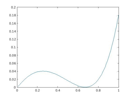
where is the function .
Since the region (6) is compact, and the inequality (7) is already known on the boundary of this region, it suffices to verify (7) when is a critical point of the left-hand side, that is to say that
Since , we can rewrite this condition as
| (8) |
The function is increasing for and decreasing for , so it can only attain any given value at most twice. From (8) and the pigeonhole principle, we conclude that at least two of are equal. Without loss of generality we may assume , then from (8) we have
and
and hence
Dividing by we obtain
and then setting we conclude that
| (9) |
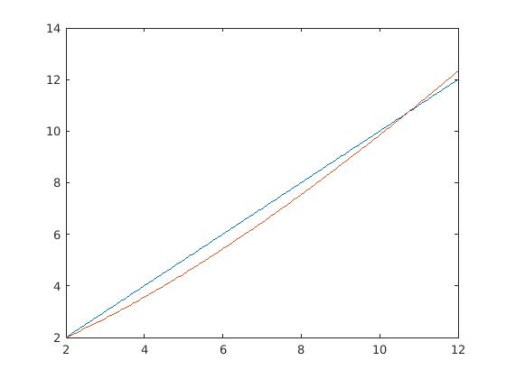
The function is convex, equals when , when , and is larger than for sufficiently large . As a consequence, the equation (9) has exactly two solutions, one at and one with ; see Figure 2. The second solution can be computed numerically as . Thus, there are two critical points with , the first of which is
and the second of which can be computed numerically as
At the first critical point, we have , and one easily verifies that the left-hand side of (7) vanishes since . At the second critical point, one can numerically verify that
and hence
at this critical point, giving the claim.
Remark 6.
The above methods extend111We thank Paata Ivanishvili for this comment. to establish the more general bound
for any , where now . In particular one has
for any finite collection of sets. We sketch the details as follows. By repeating the above arguments (and using an induction on to handle boundary cases), one needs to show that
for . We can again restrict attention to critical points, in which
As before, can take only two values, say and , leading to the equations
for some positive integers summing to . Writing and , we have the system
Differentiating the second equation once with respect to gives
and differentiating twice gives (after some algebra)
so is again a convex function of (since ), and so as before the equation has at most two solutions, including the one at and . Using the equation to implicitly define in terms of , the function
then has two critical points, including one at where the function vanishes. Direct calculation shows that this critical point is a local minimum (basically because , which in turn follows from the inequality ), so the function must be positive at the other critical point (otherwise there would be an additional critical point from the mean value theorem and intermediate value theorem), giving the claim.
2 A variant for additive energy
Recall from [9] that the additive energy of a finite subset of an additive group is defined as the number of quadruples such that . We have the trivial bound , which is attained for instance when is itself a finite group. By modifying the above arguments, we have the following refinement in the discrete cube :
Theorem 7.
Let , and let . Then , where . Furthermore, the exponent cannot be replaced by any smaller quantity.
The second claim is clear, since if then one easily computes that and . As in the previous section, the theorem is proven by induction on together with an elementary inequality, namely
Lemma 8 (Elementary inequality).
If , then
Proof.
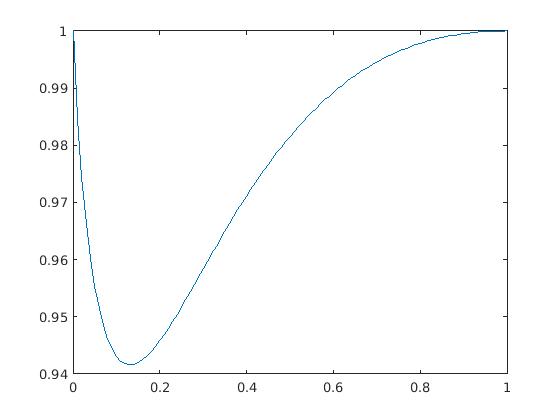
By symmetry and scaling we may assume that and , thus we need to show that
for (see Figure 3). Near , the left-hand side is and the right-hand side is at least , so the claim holds for sufficiently close to zero. At , the function takes the value of , first derivative of , and second derivative of
while takes the value of , first derivative of , and second derivative of
so the claim also holds for sufficiently close to . It thus suffices to verify the inequality at any critical point of the functional
in . Differentiating, we see that such a critical point solves the equation
which simplifies to
| (10) |
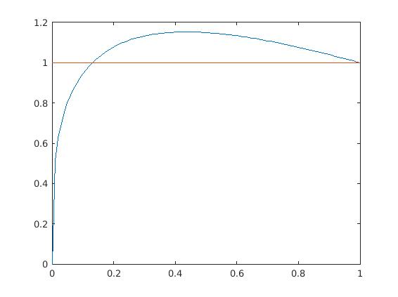
The second derivative of the left-hand side is
since and , we conclude that is strictly concave. As this function is at and at , and has a derivative of at , there are exactly two solutions to (10) for , one at and another with ; see Figure 4. The second solution can be numerically evaluated as , at which
and
giving the claim. ∎
Now we establish Theorem 7. The claim is trivial for , so suppose that and that the claim has already been proven for . For , we may partition
for some . We can then split
By the Cauchy-Schwarz inequality (and writing as ) we have
and hence by the induction hypothesis
Applying Lemma 8 and noting that , we obtain , closing the induction.
Remark 9.
The same argument shows that
for any function (where the convolution is viewed as a function on ). By several applications of the Cauchy-Schwarz inequality, this implies that
for any functions . Thus, for instance, if , the number of solutions to with is at most .
Remark 10.
In [1], the method of compressions is used to obtain optimal lower bounds for the size of a sumset of two subsets of of specified cardinality. It is possible that compression methods could also be used to obtain an alternate proof of Theorem 7, and perhaps to also refine the upper bound of slightly when is not a power of two. However, we were unable to use the method of compressions to attack Theorem 1.
3 Acknowledgments
The authors would like to thank Siavash Mirarab for bringing this problem to our attention, and David Speyer and the anonymous referee for helpful comments. DK is supported by NSF award CCF-1553288 (CAREER). TT is supported by NSF grant DMS-1266164, the James and Carol Collins Chair, and by a Simons Investigator Award.
References
- [1] B. Bollobás, I. Leader, Sums in the grid, Discrete Math. 162 (1996), no. 1–3, 31–48.
- [2] P. Diaconis, L. Saloff-Coste, Logarithmic Sobolev inequalities for finite Markov chains, The Annals of Applied Probability, 6 (1996), 695–750.
- [3] R. A. Kunze, E. M. Stein, Uniformly bounded representations and harmonic analysis of the real unimodular group, Amer. J. Math. 82 (1960), 1–62.
- [4] S. Mirarab, R. Reaz, M. S. Bayzid, T. Zimmermann, M. S. Swenson, T. Warnow, ASTRAL: genome-scale coalescent-based species tree estimation, Bioinformatics. 2014;30(17):i541-i548. doi:10.1093/bioinformatics/btu462.
- [5] S. Mirarab, T. Warnow, ASTRAL-II: coalescent-based species tree estimation with many hundreds of taxa and thousands of genes, Bioinformatics. 2015;31(12):i44-i52. doi:10.1093/bioinformatics/btv234.
- [6] M. T. Hallett, J. Lagergren, New Algorithms for the Duplication-Loss Model; 2000. doi:10.1145/332306.332359.
- [7] D. Bryant, M. Steel, Constructing Optimal Trees from Quartets, J Algorithms. 2001;38:237-259. doi:10.1006/jagm.2000.1133.
- [8] M. Lafond, C. Scornavacca, On the Weighted Quartet Consensus problem. October 2016.
- [9] T. Tao, V. Vu, Additive combinatorics. Cambridge Studies in Advanced Mathematics, 105. Cambridge University Press, Cambridge, 2006