2018 Vol. X No. XX, 000–000
33institutetext: National Astronomical Observatories, CAS, 20A Datun Road, ChaoYang District, Beijing 100101, China
44institutetext: Key Laboratory of Optical Astronomy, National Astronomical Observatories, CAS, Beijing 100101, China
\vs\no
A catalogue of 74 new open clusters found in Gaia Data-Release 2
Abstract
Based on astrometric data from Gaia Data-Release 2 (DR2), we employ an unsupervised machine learning method to blindly search for open star clusters in the Milky Way within the Galactic latitude range of . In addition to 2,080 known clusters, 74 new open cluster candidates are found. In this work, we present the positions, apparent radii, parallaxes, proper motions and member stars of these candidates 111 https://cdsarc.u-strasbg.fr/ftp/vizier.submit//new_OC/. Meanwhile, to obtain the physical parameters of each candidate cluster, stellar isochrones are fit to the photometric data. The results show that the apparent radii and the observed proper motion dispersions of these new candidates are consistent with those of open clusters previously identified in Gaia DR2.
keywords:
Galaxy: open clusters and associations–methods: data analysis–surveys1 Introduction
An open cluster (hereafter OC) is a gravitationally bound stellar system composed of dozens to thousands of stars, which presents a loose structure and is irregularly shaped (Zu & Zhao 2003). The member stars of an OC originated from the collapse of the same dense molecular environment (McKee & Ostriker 2007), and thus they have similar ages, kinematics and chemical compositions. The age of OCs can range from millions to billions of years (Dias et al. 2002; Kharchenko et al. 2013; Cantat-Gaudin et al. 2020), making them ideal places to study the evolution of stars, and they are important tracers to study the structure and kinematics of the Milky Way (e.g. Friel 1995; Lada & Lada 2003; Carraro et al. 2007; Cantat-Gaudin et al. 2020; Pang et al. 2020).
It is estimated that the total number of OCs in the Galactic disk is of the order 105 (Piskunov et al. 2006). The traditional method of identifying OCs is to use the positions and proper motions of groups of stars (e.g. Sanders 1971; Slovak 1977; Zhao & He 1990; Uribe & Brieva 1994; Sánchez et al. 2010). In addition, photometric data can be used to make a colour-magnitude diagram (CMD) of a cluster to which stellar isochrones can be fit to obtain the physical parameters of the OC, such as its age, extinction and distance modulus. Before the Gaia era, more than 3,000 OCs had been identified and catalogued using ground-based telescopes (e.g. Dias et al. 2002; Kharchenko et al. 2013).
Gaia DR2 contains accurate parallaxes and proper motions for more than one billion stars (Gaia Collaboration et al. 2018; Lindegren et al. 2018), where stars at different distances are distinguished via stellar parallaxes. Based on Gaia data, searches for OCs have yielded great results. At present, 1,500 known star clusters have been identified in Gaia DR2 (e.g. Cantat-Gaudin et al. 2018; Liu & Pang 2019); in addition, 1,100 most probable new OC candidates have been recently published (e.g. Cantat-Gaudin et al. 2018, 2019; Sim et al. 2019; Liu & Pang 2019; Castro-Ginard et al. 2018, 2019, 2020; Ferreira et al. 2019, 2020; Hao et al. 2020; Qin et al. 2020).
The continuous discovery of new OCs shows that not all existing star clusters have yet been found. In this paper, relying on the precise astrometric data of Gaia DR2, we employ an unsupervised machine learning method to carry out blind searches for clusters within . After removing 2,080 previously reported clusters, we find 74 new OC candidates and obtain their physical parameters.
The remainder of this paper is organised as follows. In Section 2 we introduced the data. Section 3 presents our methods, including data preprocessing, the clustering algorithm and the isochrone fitting. Section 4 presents the results and provides discussions, and the conclusions are summarised in Section 5.
2 Data
The Gaia satellite was launched by the European Space Agency in 2013, and its first data release was in 2016 (Gaia Collaboration et al. 2016). DR2 (Gaia Collaboration et al. 2018) provided high-precision positions and -band photometric data of approximately 1.7 billion sources, of which 1.4 billion sources have both and magnitudes, and 1.3 billion stars have measured parallaxes and proper motions.
Previous studies reported that most known OCs are located near the Galactic plane (e.g. Dias et al. 2002; Kharchenko et al. 2013). Hence, we applied three selection cuts to the Gaia DR2 catalogue:
-
•
,
-
•
0.2 mas, parallaxovererror > 1,
-
•
mag.
Thus, stars with mag and which possess a parallax uncertainty of 0.2 mas or better were added to our sample, as previously used by Cantat-Gaudin et al. (2018, 2020); Liu & Pang (2019); Ferreira et al. (2020). The final sample contained 169,137,482 stars with astrometric parameters , where 166,136,789 had photometric data (, , ).
3 Method
We used the stellar astrometric and photometric data derived in Section 2 to search for and identify new star clusters. The main method used is as follows:
-
•
Preprocess the astrometric data ;
-
•
Fit NND (see Section 3.2.2) to obtain the clustering parameters, and use the clustering algorithm to obtain cluster groups; and
-
•
Fit stellar isochrones to the photometric data (, -) of the cluster candidates.
3.1 Astrometric data preparing
Following the same approach as Hao et al. (2020), the regions containing the data (as identified in Section 2) were divided into rectangles of size and . Considering that the positions and proper motions are relative parameters, i.e. the absolute values of distances and proper motions of stars with different parallaxes are variational, we used the projected positions, parallaxes and decomposed proper motions as input data for the clustering analysis as:
| (1) |
where the distance is taken to be the inverse of the parallax, while () and are the angular sizes of the star and the centre of the rectangle in and , respectively. In addition, we calculated the median dispersion of () for the 2,017 OCs catalogued by Cantat-Gaudin et al. (2020) to standardize the above input data, so that the values in each dimension were multiples of the median dispersion of the corresponding parameter, and thus the weights of the input parameters in the process were equalized. Next, we used the DBSCAN algorithm to find clustered groups of stars.
3.2 Clustering algorithm
3.2.1 DBSCAN
The unsupervised machine learning method DBSCAN used in this work was derived from scikit-learn (Pedregosa et al. 2011). This algorithm was used to distinguish high-density groups from low-density regions in -dimensional samples (Ester et al. 1996), including extracting the core members and border members located in different groups, and rejecting any outliers not located in any group. There are two parameters in the algorithm: the minimum number of data points and the radius , of which the latter was measured by a distance function as follows:
| (2) |
where is the distance between data points and .
A core is defined as a sub-sample of the data set where neighbours exist within a distance equal to ; that is, the core members are located in a dense area of vector space. Border members themselves do not form cores, but they may be located close to core members (i.e. < ). In addition, outliers cannot constitute a core sample, nor can a candidate be composed of just border members, and they must be located at least from any core member. A larger or a smaller means a higher density required to form a group.
3.2.2 Clustering parameters: and
The parameter mainly controls the tolerance to outliers in this algorithm. Schubert et al. (2017) found that has a weak effect on the clustering results. Sander et al. (1998) suggested that can be determined as twice the value of the dimension of the data set; that is, =2 , where = 5 in this work. We tried different values of around 10, and found that the detection efficiency was highest when using , that is, we could obtain more cores without obvious outliers. At the same time, this value was also within the range of the best values of used by Castro-Ginard et al. (2018); Hao et al. (2020). We present the results of = 8 in this article.
The parameter controls the radius of the local area of the points in the data set, and cannot be set to the default value (Schubert et al. 2017; Castro-Ginard et al. 2018). When this parameter is too small, most of the data will not be clustered; when it is too large, any adjacent clusters or outliers will merge into one group. In previous studies, Ester et al. (1996); Sander et al. (1998) selected based on the nearest neighbour distance (NND). On this basis, Schubert et al. (2017) obtained the corresponding value by observing the significant change of sorted NND plot. In the algorithm of NND, the reference point is not specified as a neighbor, while that is included in the DBSCAN for density estimation, so the value used in this work is = -1.
In this work, the main steps to get are:
-
•
Compute the NND histogram via 111 https://github.com/scikit-learn/scikit-learn.
-
•
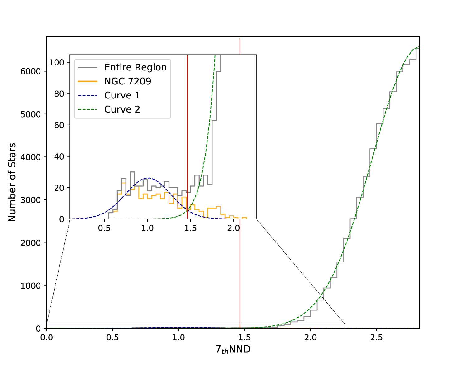
Fit the NND using a bimodal Gaussian function. For gravitationally bound systems such as OCs, the intervals between the member stars in position and proper motion vectors are closer than those of field stars, so their NNDs are significantly smaller than those of field stars (Castro-Ginard et al. 2018). In the NND histogram, the NND of the cluster is distributed on the leftmost end (i.e. the minimum end, Fig. 1) of the whole data set. Inspired by Castro-Ginard et al. (2018), in this work, we used a fitted NND histogram to determine as:
(3) where is the statistical number of NND, is the distance, the fitted range of is (0, [n=max (n)]), and are coefficients of the Gaussian functions. As shown in Fig. 1, we used two functions (curves 1 and 2) obtained by Eq. 3 to fit the NND histogram. For a data set that contains any contributions from OCs, we found that the two Gaussian functions have a real number solution (e.g. the vertical red line in Fig. 1), and it is set to be the value used in DBSCAN.
3.3 Isochrone fitting
To estimate the physical parameters of the cluster candidates, we fit isochrones to the CMDs derived from the member stars of the clusters. The isochrones used here contain logarithmic ages from 5.92 to 10.12 with a step of 0.02, and metal fractions from 0.015 to 0.029 with a step of 0.001 111 http://stev.oapd.inaf.it/cgi-bin/cmd, which come from the PARSEC library (Bressan et al. 2012) and have been updated for the Gaia DR2 passbands using the photometric calibrations of Evans et al. (2018). The isochrones were corrected for extinction and reddening, using an extinction curve with = 3.1 (Cardelli et al. 1989; O’Donnell 1994).
We selected clusters whose CMDs appeared to best-fit the theoretical isochrones. Following the method of Liu & Pang (2019), the mean square distances to the isochrones were used to match the observed cluster members using Eq. 4:
| (4) |
where is the number of core members (Section 3.2.1) in a cluster, and , are the positions of the member stars and the points on the isochrone that are closest to the member stars, respectively. At the same time, we also obtained the standard deviation of the square distance, , which was used to reflect the dispersion of the core members along the isochrones (Section 4.2).
4 Results and discussion
We applied the algorithm described in Section 3.2.1 to about 170 million stars. Since some clusters were located near the edges of each rectangle (Section 3.1), in order not to find duplicate clusters or substructures of known clusters, we merged the cluster results within a range of 3 of the astrometric data ; meanwhile, a visual inspection was also adopted. Moreover, to reduce the influence of outliers, we omitted clustering results with < 5. After that, we obtained 3,066 groups with a total of 371,362 members, of which 261,377 were core members. Thereafter, we removed all known OCs from this sample (Section 4.1).
4.1 Cross matching with previous catalogues
4.1.1 OCs in Gaia DR2
Our first cross-matched catalogue contained OCs derived from Gaia DR2. In the previous studies, Sim et al. (2019) found 207 new OCs within 1 kpc of solar system, while Liu & Pang (2019) found 2,443 star clusters and candidates, 76 of which were most probable new star clusters. Cantat-Gaudin et al. (2020) re-visited 2017 OCs, including the catalogues of Cantat-Gaudin et al. (2018, 2019); Cantat-Gaudin & Anders (2020); Castro-Ginard et al. (2018, 2019, 2020), and a portion of OCs published by Sim et al. (2019); Liu & Pang (2019). In addition, we considered the 28, 16 and four new OCs recently been found by Ferreira et al. (2019, 2020); Hao et al. (2020); Qin et al. (2020), respectively.
Most OCs are observed to have projected spatial extents up to nearly 15 pc (Gaia Collaboration et al. 2017) from the cluster centres, such as the apparent radii of OCs found in Gaia DR2 by Cantat-Gaudin & Anders (2020). Therefore, within the range of the maximum distance from the centre of an OC considered here (15 pc, 5 dispersion) within , we extracted the reported clusters adjacent to the center of each identified group. Then, in the range of a 5 dispersion about , the extracted clusters were matched, and the matched ones were removed. Finally, a total of 1,978 reported star clusters were removed.
4.1.2 OCs before Gaia
We continue to match the remaining groups with the catalogues published by Dias et al. (2002, D02) and Kharchenko et al. (2013, K13). To do this we made use of the root mean square (RMS) differences of the ages and distance moduli between the K13 clusters and cross-matched clusters identified in Gaia DR2 by Cantat-Gaudin et al. (2020), which reflected the differences of these parameters between the re-identified clusters in Gaia DR2 and the previous known OCs. We selected clusters in a range of max(15 pc, 5 dispersion) about , and then compared the ages and distance moduli of the remaining groups with those of the K13 and D02 clusters within a 2-RMS level. In all, 46 groups were removed.
Next, Bica et al. (2019, B19) constructed a sample 4,384 open/globular clusters, cluster candidates and cluster remnants, where most of them were previously catalogued by D02 and K13. We also matched the objects found by B19 with the remaining groups, where the radius of each matched cluster had to satisfy , where is the angular size between the matched group and the reported cluster. Although most star clusters could be physically distinguished, we also performed visual checks of the groups and reported clusters. In the end, we found that some groups were closely matched with the centre positions catalogued by B19, and we included two of them in the final table (Table LABEL:tab1). After all the checking and filtering, 986 groups remained in our collated sample.
4.2 New cluster candidates
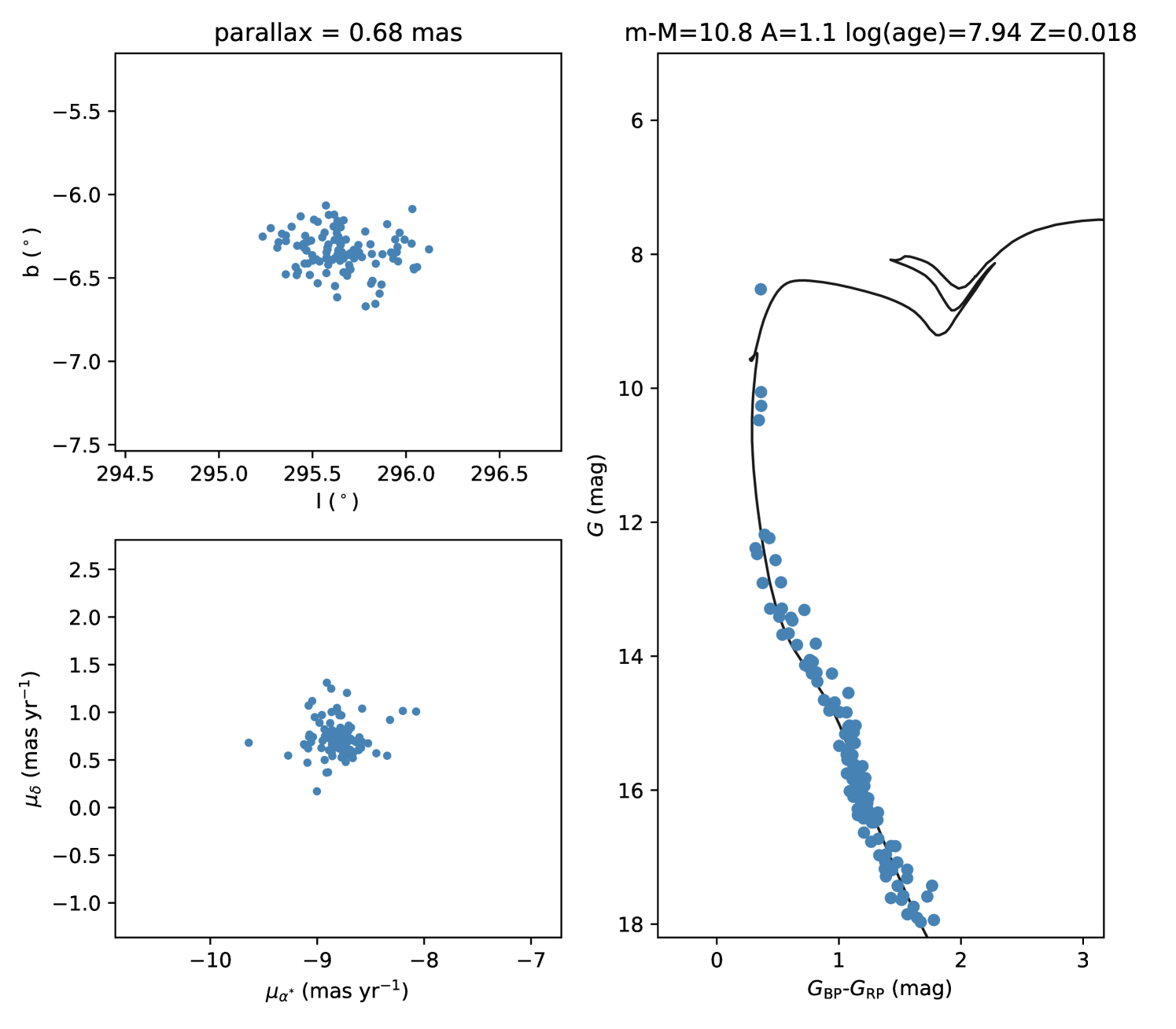
To find any probable new star clusters among the 986 groups, we selected clusters whose CMDs coincided well with the stellar isochrones (Section 3.3). Inspired by Liu & Pang (2019), we first adopted criteria of . After application of these criteria, 168 clusters with well-fitting isochrones remained in the sample. Furthermore, we performed visual inspections under careful consideration of the distributions of the positions and proper motions, and the CMDs of the remaining clusters. After that, 74 OC candidates remained. In Table LABEL:tab1, we have presented the locations and sizes of these candidates, including their parallaxes, proper motions and corresponding 1 dispersions, which have also been presented in the works of Cantat-Gaudin & Anders (2020); Cantat-Gaudin et al. (2020) in the same way. The distance moduli, ages, extinction and metal fraction values of these candidates are also provided. The distributions, proper motions, CMDs (e.g. Fig. 2) and member stars of each cluster are also shown in electric form.
| NO. | ) | log(age/yr) | |||||||||
| (∘) | (∘) | (deg) | (mas) | (mas yr-1) | (mas yr-1) | (mag) | (mag) | ||||
| 001 | 94.203 | -5.840 | 0.20 | 45(20) | 0.67(0.03) | 1.28(0.16) | -2.34(0.12) | 10.9 | 8.40 | 1.0 | 0.016 |
| 002 | 215.533 | 4.061 | 0.11 | 44(22) | 0.50(0.05) | -0.51(0.11) | -1.48(0.11) | 11.5 | 8.12 | 0.9 | 0.025 |
| 003 | 237.912a | 0.449 | 0.18 | 143(75) | 0.55(0.05) | -1.38(0.13) | 1.24(0.13) | 11.4 | 8.36 | 0.6 | 0.026 |
| 004 | 116.192 | -1.297 | 0.09 | 32(15) | 0.37(0.03) | -1.78(0.09) | -1.02(0.06) | 12.0 | 7.82 | 2.2 | 0.021 |
| 005 | 228.825 | 1.196 | 0.26 | 32(15) | 1.18(0.03) | -1.41(0.18) | 0.44(0.26) | 9.7 | 8.04 | 0.4 | 0.028 |
| 006 | 354.888 | -1.335 | 0.14 | 70(45) | 1.05(0.05) | 1.12(0.12) | -0.09(0.11) | 9.3 | 8.84 | 0.3 | 0.025 |
| 007 | 11.026 | -1.960 | 0.13 | 52(25) | 0.79(0.05) | -0.06(0.13) | -1.62(0.12) | 10.5 | 7.48 | 0.9 | 0.024 |
| 008 | 87.492a | -3.675 | 0.37 | 50(24) | 0.85(0.04) | 0.05(0.14) | -4.35(0.13) | 10.4 | 8.54 | 1.0 | 0.027 |
| 009 | 241.773 | 0.143 | 0.17 | 41(13) | 0.38(0.03) | -1.63(0.09) | 1.31(0.12) | 11.9 | 7.98 | 0.6 | 0.026 |
| 010 | 339.546 | -4.429 | 0.22 | 67(45) | 1.09(0.05) | -1.33(0.14) | -2.67(0.15) | 9.9 | 7.98 | 1.0 | 0.027 |
| 011 | 261.833 | -9.192 | 0.43 | 101(39) | 0.63(0.04) | -3.79(0.18) | 4.92(0.18) | 11.3 | 7.44 | 0.9 | 0.024 |
| 012 | 202.447 | -5.870 | 0.23 | 54(28) | 0.86(0.06) | -0.01(0.18) | -1.43(0.17) | 10.4 | 7.58 | 0.9 | 0.021 |
| 013 | 315.674 | 1.631 | 0.25 | 57(36) | 0.87(0.04) | -1.20(0.10) | -3.11(0.13) | 10.3 | 7.54 | 1.1 | 0.017 |
| 014 | 314.563 | 2.660 | 0.15 | 46(16) | 0.52(0.02) | -2.66(0.12) | -2.72(0.10) | 11.3 | 8.52 | 0.8 | 0.027 |
| 015 | 259.105 | -2.451 | 0.24 | 81(41) | 0.70(0.04) | -5.76(0.14) | 4.21(0.14) | 10.9 | 8.02 | 1.1 | 0.027 |
| 016 | 295.638 | -6.345 | 0.21 | 107(63) | 0.68(0.04) | -8.80(0.13) | 0.72(0.14) | 10.8 | 7.94 | 1.1 | 0.018 |
| 017 | 226.571 | 0.150 | 0.24 | 43(21) | 0.93(0.07) | -2.11(0.19) | -0.18(0.13) | 10.3 | 8.42 | 0.7 | 0.024 |
| 018 | 165.573 | -2.123 | 0.30 | 46(19) | 0.95(0.07) | -0.40(0.17) | -3.05(0.14) | 9.9 | 7.54 | 0.9 | 0.019 |
| 019 | 210.343 | -4.082 | 0.14 | 41(24) | 0.76(0.05) | 1.44(0.10) | -1.31(0.10) | 10.6 | 8.60 | 1.5 | 0.017 |
| 020 | 303.139 | -0.852 | 0.09 | 59(28) | 0.63(0.07) | -6.34(0.19) | -1.58(0.14) | 10.6 | 7.94 | 1.7 | 0.024 |
| 021 | 224.698 | 3.430 | 0.11 | 46(19) | 0.46(0.06) | -0.80(0.12) | -0.87(0.11) | 11.1 | 9.02 | 0.1 | 0.019 |
| 022 | 224.178 | 1.248 | 0.22 | 47(30) | 0.86(0.06) | -0.57(0.11) | 0.83(0.20) | 10.5 | 7.76 | 0.7 | 0.016 |
| 023 | 102.341 | -2.235 | 0.10 | 38(26) | 0.68(0.04) | 1.71(0.09) | -2.25(0.13) | 11.0 | 8.72 | 1.1 | 0.028 |
| 024 | 236.831 | 2.172 | 0.10 | 39(27) | 0.59(0.05) | -0.99(0.07) | 0.59(0.10) | 11.2 | 7.96 | 1.0 | 0.025 |
| 025 | 312.078 | -2.372 | 0.06 | 34(14) | 0.48(0.03) | -4.72(0.08) | -3.13(0.15) | 11.2 | 7.60 | 1.2 | 0.021 |
| 026 | 240.457 | -4.731 | 0.31 | 85(55) | 0.80(0.05) | -4.29(0.13) | 3.85(0.11) | 10.5 | 7.44 | 0.1 | 0.026 |
| 027 | 333.864 | -4.275 | 0.13 | 32(13) | 0.59(0.01) | -1.58(0.14) | -4.01(0.07) | 11.1 | 8.66 | 1.1 | 0.028 |
| 028 | 100.808 | 0.620 | 0.14 | 88(42) | 0.64(0.05) | -2.01(0.16) | -1.63(0.12) | 10.8 | 7.92 | 2.2 | 0.027 |
| 029 | 2.373 | -0.261 | 0.22 | 63(45) | 1.66(0.05) | 0.89(0.19) | -5.12(0.18) | 9.0 | 7.70 | 0.8 | 0.023 |
| 030 | 24.838 | -6.092 | 0.22 | 43(27) | 0.94(0.04) | 1.13(0.11) | 0.84(0.10) | 10.3 | 8.50 | 1.1 | 0.026 |
| 031 | 86.396 | -0.476 | 0.04 | 33(16) | 0.49(0.03) | -2.51(0.13) | -4.52(0.14) | 11.0 | 8.14 | 1.7 | 0.020 |
| 032 | 221.101 | -1.049 | 0.19 | 51(30) | 0.88(0.04) | -1.59(0.13) | -3.46(0.14) | 10.5 | 8.54 | 0.8 | 0.025 |
| 033 | 343.054 | 2.668 | 0.18 | 100(56) | 0.90(0.05) | 1.42(0.19) | -2.98(0.16) | 10.1 | 7.64 | 1.2 | 0.016 |
| 034 | 309.876 | 1.271 | 0.14 | 41(27) | 0.75(0.04) | -7.20(0.09) | -2.26(0.11) | 10.4 | 7.98 | 0.8 | 0.025 |
| 035 | 161.079 | -0.654 | 0.09 | 34(17) | 0.52(0.05) | 1.43(0.13) | -2.11(0.26) | 11.5 | 8.44 | 1.0 | 0.024 |
| 036 | 263.281 | -6.758 | 0.27 | 32(15) | 0.93(0.04) | -5.61(0.15) | 5.11(0.15) | 10.1 | 7.88 | 0.4 | 0.027 |
| 037 | 20.457 | -0.866 | 0.15 | 37(19) | 0.92(0.05) | -0.06(0.14) | -3.05(0.12) | 9.9 | 8.82 | 1.4 | 0.023 |
| 038 | 178.173 | 2.255 | 0.15 | 30(14) | 0.71(0.05) | 0.49(0.15) | -3.81(0.10) | 10.8 | 8.46 | 0.7 | 0.026 |
| 039 | 121.599 | 6.001 | 0.33 | 37(21) | 0.96(0.03) | -1.53(0.14) | -0.57(0.11) | 9.5 | 7.94 | 1.9 | 0.016 |
| 040 | 70.424 | -1.231 | 0.03 | 50(38) | 0.48(0.03) | -3.83(0.09) | -5.30(0.14) | 11.1 | 8.24 | 3.9 | 0.024 |
| 041 | 92.224 | -6.323 | 0.61 | 68(29) | 0.78(0.04) | 2.15(0.24) | -0.02(0.11) | 10.2 | 8.88 | 0.4 | 0.017 |
| 042 | 252.836 | -1.370 | 0.31 | 66(36) | 0.86(0.04) | -4.78(0.10) | 2.97(0.15) | 10.4 | 7.96 | 0.7 | 0.026 |
| 043 | 237.960 | 0.637 | 0.19 | 90(41) | 0.66(0.04) | -2.52(0.18) | 1.65(0.12) | 10.9 | 8.46 | 0.3 | 0.026 |
| 044 | 134.977 | 1.725 | 0.18 | 34(20) | 0.67(0.03) | -0.91(0.18) | -0.46(0.13) | 10.8 | 7.66 | 1.8 | 0.017 |
| 045 | 111.351 | -2.453 | 0.14 | 59(40) | 0.99(0.04) | -0.42(0.12) | -0.83(0.12) | 9.9 | 7.90 | 2.2 | 0.020 |
| 046 | 68.596 | 2.636 | 0.09 | 56(37) | 0.49(0.04) | -2.51(0.10) | -3.43(0.11) | 11.3 | 8.34 | 1.7 | 0.018 |
| 047 | 327.232 | -1.331 | 0.07 | 33(11) | 0.57(0.03) | -3.95(0.16) | -5.16(0.11) | 10.6 | 8.78 | 2.0 | 0.024 |
| 048 | 225.173 | 5.548 | 0.15 | 33(17) | 0.90(0.08) | -3.59(0.14) | 0.99(0.11) | 10.2 | 7.98 | 0.1 | 0.026 |
| 049 | 169.769 | -1.966 | 0.13 | 33(17) | 0.60(0.04) | 1.15(0.13) | -3.97(0.09) | 10.9 | 8.18 | 1.2 | 0.024 |
| 050 | 203.158 | -2.565 | 0.07 | 41(20) | 0.49(0.05) | -0.90(0.16) | -0.24(0.10) | 11.7 | 8.16 | 1.0 | 0.019 |
| 051 | 19.445 | -2.247 | 0.08 | 45(23) | 0.56(0.04) | 0.67(0.11) | -0.14(0.11) | 10.9 | 8.10 | 1.9 | 0.025 |
| 052 | 220.279 | 0.592 | 0.17 | 35(20) | 0.60(0.04) | -0.26(0.11) | -0.64(0.16) | 10.7 | 7.92 | 0.5 | 0.021 |
| 053 | 174.786 | -1.207 | 0.14 | 35(13) | 0.64(0.06) | 1.41(0.17) | -3.54(0.18) | 11.2 | 7.54 | 1.1 | 0.023 |
| 054 | 221.571 | 0.052 | 0.16 | 50(33) | 0.93(0.02) | -3.94(0.15) | 1.14(0.14) | 10.3 | 8.42 | 0.4 | 0.028 |
| 055 | 298.570 | -8.573 | 0.35 | 42(18) | 0.73(0.05) | -4.05(0.16) | -0.69(0.13) | 10.5 | 7.78 | 0.9 | 0.017 |
| 056 | 92.545 | -3.423 | 0.10 | 34(18) | 0.78(0.05) | 1.44(0.08) | -0.35(0.11) | 10.6 | 7.90 | 0.9 | 0.027 |
| 057 | 16.639 | -1.919 | 0.13 | 40(19) | 0.86(0.05) | -2.70(0.08) | -3.56(0.08) | 10.1 | 8.48 | 0.7 | 0.028 |
| 058 | 203.355 | 0.556 | 0.12 | 38(15) | 0.48(0.04) | 0.03(0.11) | -1.38(0.07) | 11.3 | 7.28 | 1.1 | 0.018 |
| 059 | 235.209 | 1.629 | 0.06 | 35(20) | 0.41(0.04) | -2.23(0.10) | 2.19(0.09) | 12.0 | 7.52 | 1.5 | 0.021 |
| 060 | 210.929 | 5.473 | 0.13 | 55(29) | 0.48(0.04) | -0.39(0.11) | -1.66(0.12) | 11.5 | 8.30 | 0.9 | 0.022 |
| 061 | 221.759 | -4.652 | 0.14 | 73(37) | 0.50(0.04) | -1.28(0.12) | 1.25(0.15) | 11.6 | 8.28 | 1.4 | 0.020 |
| 062 | 233.570 | -4.761 | 0.10 | 36(14) | 0.49(0.05) | -1.60(0.14) | 0.67(0.13) | 11.3 | 8.38 | 1.6 | 0.024 |
| 063 | 133.389 | -0.837 | 0.08 | 39(21) | 0.63(0.06) | -0.89(0.09) | 0.16(0.18) | 10.8 | 8.00 | 2.1 | 0.022 |
| 064 | 293.050 | -6.779 | 0.28 | 46(27) | 0.93(0.04) | -7.41(0.14) | 1.72(0.19) | 10.2 | 7.90 | 1.0 | 0.022 |
| 065 | 245.796 | 3.234 | 0.19 | 32(23) | 0.99(0.04) | -3.93(0.11) | 2.00(0.10) | 10.1 | 8.20 | 0.2 | 0.028 |
| 066 | 14.837 | 1.394 | 0.05 | 33(13) | 0.61(0.03) | -0.25(0.12) | -1.73(0.15) | 11.4 | 6.80 | 1.4 | 0.028 |
| 067 | 323.479 | -2.512 | 0.06 | 33(16) | 0.54(0.03) | -2.17(0.07) | -3.52(0.11) | 10.7 | 8.38 | 1.8 | 0.028 |
| 068 | 262.909 | -4.363 | 0.38 | 71(31) | 0.82(0.05) | -6.29(0.20) | 5.02(0.33) | 10.3 | 7.78 | 0.7 | 0.017 |
| 069 | 234.158 | -12.181 | 0.33 | 93(66) | 0.94(0.06) | -1.52(0.12) | 2.45(0.15) | 10.1 | 8.60 | 0.4 | 0.018 |
| 070 | 254.535 | -6.050 | 0.28 | 31(11) | 0.82(0.05) | -4.06(0.16) | 4.59(0.21) | 10.3 | 7.98 | 0.6 | 0.027 |
| 071 | 255.762 | -4.530 | 0.14 | 36(18) | 0.67(0.04) | -4.20(0.14) | 3.38(0.08) | 11.1 | 8.52 | 1.2 | 0.028 |
| 072 | 217.519 | 0.474 | 0.22 | 35(12) | 0.64(0.04) | -0.15(0.09) | -0.80(0.10) | 11.3 | 7.86 | 0.5 | 0.028 |
| 073 | 147.486 | 4.112 | 0.15 | 68(36) | 0.69(0.06) | 1.04(0.10) | -1.06(0.15) | 10.4 | 7.82 | 2.1 | 0.018 |
| 074 | 216.760 | -0.834 | 0.05 | 35(20) | 0.42(0.05) | -1.81(0.11) | 1.07(0.07) | 11.6 | 8.76 | 1.2 | 0.019 |
-
•
a Adjacent to the cluster catalogued by Bica et al. (2019).
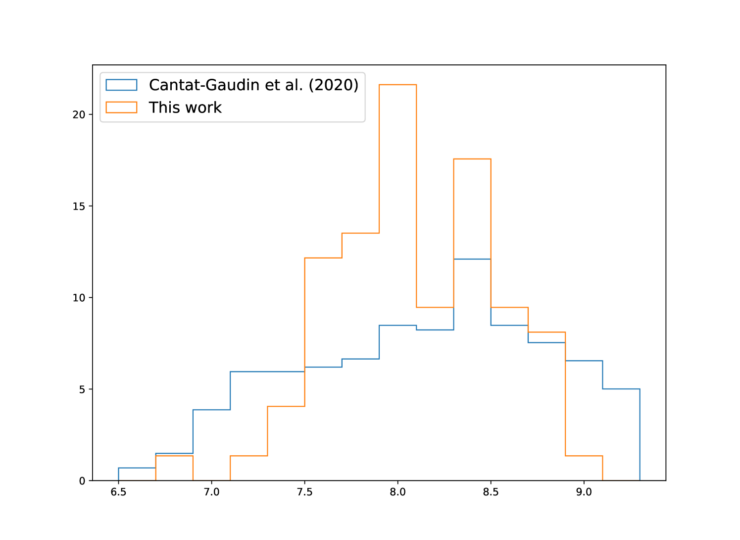
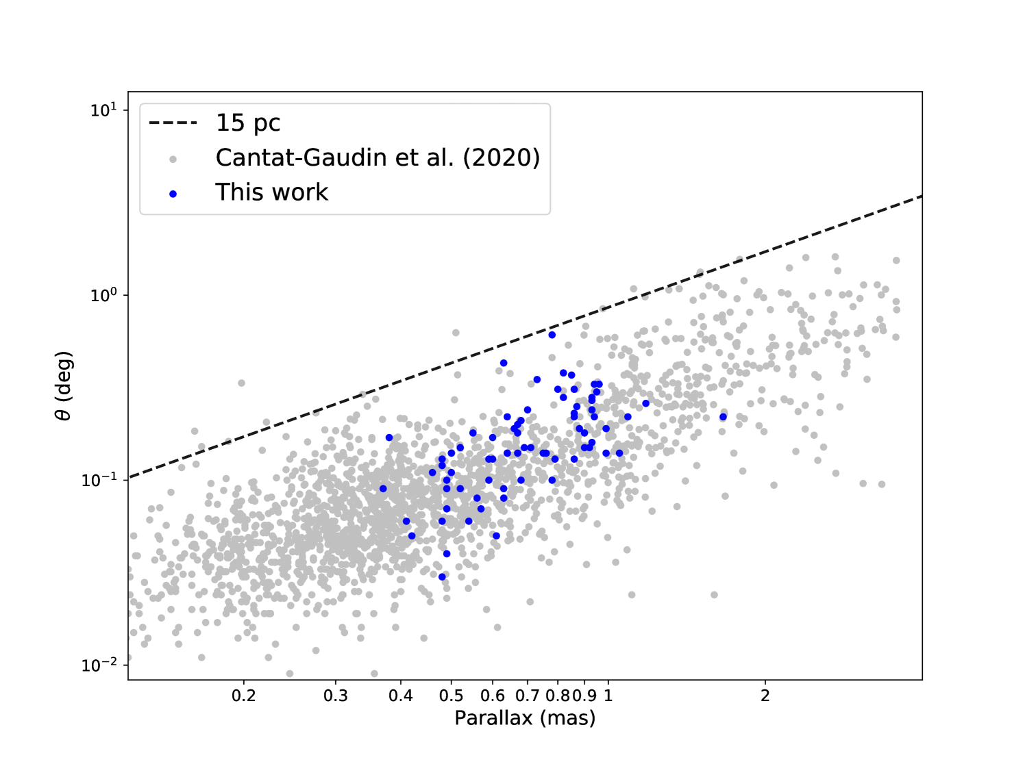
As shown in Fig. 3, the isochrones show that the ages of most of the new OC candidates are in the range of log (age/yr) = (7.5, 8.5), and two extreme values are located at log (age/yr) = 8.0 and 8.4. These results are similar to the age distributions of the OCs presented by Cantat-Gaudin et al. (2020, CG20). However, the peak value of log (age/yr) = 8.0 may be due to bias caused by the new cluster candidates found in this work forming an incomplete sample. In addition, as shown in Fig. 4, the apparent radii of the new star cluster candidates are below 15 pc, which is consistent with the distributions of apparent radii of OCs catalogued by CG20.
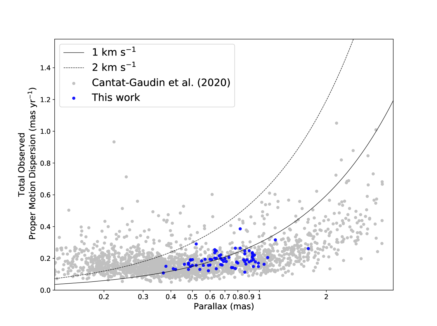
As a gravitationally bound system, member stars of an OC have much smaller internal velocity dispersions than field stars. Radial velocities derived from high-resolution spectroscopic observations have shown that the internal velocity dispersion of OCs are generally less than 2 km s-1(e.g. Donati et al. 2014; Cantat-Gaudin et al. 2014; Vereshchagin & Chupina 2016; Overbeek et al. 2017). Meanwhile, the observed proper motion dispersions of the clusters found in Gaia DR2 are correlated with their parallaxes (Cantat-Gaudin & Anders 2020; Ferreira et al. 2020). As shown in Fig. 5, the proper motion dispersions of the new star cluster candidates found in this work are below 0.5 mas yr-1, and the resolved velocity dispersions of most candidates are below 1 km s-1, which are consistent with the results of star clusters found in Gaia DR2 by Cantat-Gaudin et al. (2020).
5 Conclusion
Adopting the clustering algorithm DBSCAN, we used the positions, parallaxes, and proper motions of nearly 170 million stars within the galactic latitude range and parallax 0.2 mas in Gaia DR2 to search for unknown OCs. We cross-matched our initial sample with previous star cluster catalogues, and after performing several vetting stages, we obtained a catalogue of 74 new OC candidates. We fitted isochrones to these candidates and obtained their corresponding physical parameters. The apparent radii and observed proper motion dispersions of the new cluster candidates were consistent with those of OCs previously found in Gaia DR2.
The detection of new OC candidates shows that there are still some missed OCs in the Gaia data. Gaia EDR3 will be initially released in December 2020, with the complete release due the first half of 2022, which will contain higher precision parallaxes, proper motions and photometric data. Therefore, the newly discovered OC candidates in this work can be further confirmed their natures, and more star clusters are expected to be found in future works.
6 Acknowledgements
This work has made use of data from the European Space Agency (ESA) mission Gaia(https://www.cosmos.esa.int/Gaia), processed by the Gaia Data Processing and Analysis Consortium (DPAC, https://www.cosmos.esa.int/web/Gaia/dpac/consortium). Funding for the DPAC has been provided by national institutions, in particular the institutions participating in the Gaia Multilateral Agreement. This work was funded by the NSFC (grant numbers 11933011, 11873019, and 11673066), and by the Key Laboratory for Radio Astronomy. This research has made use of the open-source Python packages Astropy (Price-Whelan et al. 2018), NumPy (Oliphant 2006), scikit-learn (Pedregosa et al. 2011) and Pandas (McKinney et al. 2010). The figures in this article were created using Matplotlib (Hunter 2007).
References
- Bica et al. (2019) Bica, E., Pavani, D. B., Bonatto, C. J., & Lima, E. F. 2019, AJ, 157, 12
- Bressan et al. (2012) Bressan, A., Marigo, P., Girardi, L., et al. 2012, MNRAS, 427, 127
- Cantat-Gaudin & Anders (2020) Cantat-Gaudin, T., & Anders, F. 2020, A&A, 633, A99
- Cantat-Gaudin et al. (2014) Cantat-Gaudin, T., Vallenari, A., Zaggia, S., et al. 2014, A&A, 569, A17
- Cantat-Gaudin et al. (2018) Cantat-Gaudin, T., Jordi, C., Vallenari, A., et al. 2018, A&A, 618, A93
- Cantat-Gaudin et al. (2019) Cantat-Gaudin, T., Krone-Martins, A., Sedaghat, N., et al. 2019, A&A, 624, A126
- Cantat-Gaudin et al. (2020) Cantat-Gaudin, T., Anders, F., Castro-Ginard, A., et al. 2020, A&A, 640, A1
- Cardelli et al. (1989) Cardelli, J. A., Clayton, G. C., & Mathis, J. S. 1989, ApJ, 345, 245
- Carraro et al. (2007) Carraro, G., Geisler, D., Villanova, S., Frinchaboy, P. M., & Majewski, S. R. 2007, A&A, 476, 217
- Castro-Ginard et al. (2019) Castro-Ginard, A., Jordi, C., Luri, X., Cantat-Gaudin, T., & Balaguer-Núñez, L. 2019, A&A, 627, A35
- Castro-Ginard et al. (2018) Castro-Ginard, A., Jordi, C., Luri, X., et al. 2018, A&A, 618, A59
- Castro-Ginard et al. (2020) —. 2020, A&A, 635, A45
- Dias et al. (2002) Dias, W. S., Alessi, B. S., Moitinho, A., & Lépine, J. R. D. 2002, A&A, 389, 871
- Donati et al. (2014) Donati, P., Cantat Gaudin, T., Bragaglia, A., et al. 2014, A&A, 561, A94
- Ester et al. (1996) Ester, M., Kriegel, H.-P., Sander, J., & Xu, X. 1996, in Proc. of 2nd International Conference on Knowledge Discovery and Data Mining (KDD-96), 226–231
- Evans et al. (2018) Evans, D. W., Riello, M., De Angeli, F., et al. 2018, A&A, 616, A4
- Ferreira et al. (2020) Ferreira, F. A., Corradi, W. J. B., Maia, F. F. S., Angelo, M. S., & Santos, J. F. C., J. 2020, MNRAS, 496, 2021
- Ferreira et al. (2019) Ferreira, F. A., Santos, J. F. C., Corradi, W. J. B., Maia, F. F. S., & Angelo, M. S. 2019, MNRAS, 483, 5508
- Friel (1995) Friel, E. D. 1995, ARA&A, 33, 381
- Gaia Collaboration et al. (2016) Gaia Collaboration, Prusti, T., de Bruijne, J. H. J., et al. 2016, A&A, 595, A1
- Gaia Collaboration et al. (2017) Gaia Collaboration, van Leeuwen, F., Vallenari, A., et al. 2017, A&A, 601, A19
- Gaia Collaboration et al. (2018) Gaia Collaboration, Brown, A. G. A., Vallenari, A., et al. 2018, A&A, 616, A1
- Hao et al. (2020) Hao, C., Xu, Y., Wu, Z., He, Z., & Bian, S. 2020, PASP, 132, 034502
- Hunter (2007) Hunter, J. D. 2007, Computing in science & engineering, 9, 90
- Kharchenko et al. (2013) Kharchenko, N. V., Piskunov, A. E., Schilbach, E., Röser, S., & Scholz, R. D. 2013, A&A, 558, A53
- Lada & Lada (2003) Lada, C. J., & Lada, E. A. 2003, ARA&A, 41, 57
- Lindegren et al. (2018) Lindegren, L., Hernández, J., Bombrun, A., et al. 2018, A&A, 616, A2
- Liu & Pang (2019) Liu, L., & Pang, X. 2019, ApJS, 245, 32
- McKee & Ostriker (2007) McKee, C. F., & Ostriker, E. C. 2007, ARA&A, 45, 565
- McKinney et al. (2010) McKinney, W., et al. 2010, in Proceedings of the 9th Python in Science Conference, Vol. 445, Austin, TX, 51–56
- O’Donnell (1994) O’Donnell, J. E. 1994, ApJ, 422, 158
- Oliphant (2006) Oliphant, T. E. 2006, A guide to NumPy, Vol. 1 (Trelgol Publishing USA)
- Overbeek et al. (2017) Overbeek, J. C., Friel, E. D., Donati, P., et al. 2017, A&A, 598, A68
- Pang et al. (2020) Pang, X., Li, Y., Tang, S.-Y., Pasquato, M., & Kouwenhoven, M. B. N. 2020, ApJ, 900, L4
- Pedregosa et al. (2011) Pedregosa, F., Varoquaux, G., Gramfort, A., et al. 2011, Journal of Machine Learning Research, 12, 2825
- Piskunov et al. (2006) Piskunov, A. E., Kharchenko, N. V., Röser, S., Schilbach, E., & Scholz, R. D. 2006, A&A, 445, 545
- Price-Whelan et al. (2018) Price-Whelan, A. M., Sipőcz, B., Günther, H., et al. 2018, The Astronomical Journal, 156, 123
- Qin et al. (2020) Qin, S.-m., Li, J., Chen, L., & Zhong, J. 2020, arXiv e-prints, arXiv:2008.07164
- Sánchez et al. (2010) Sánchez, N., Vicente, B., & Alfaro, E. J. 2010, A&A, 510, A78
- Sander et al. (1998) Sander, J., Ester, M., Kriegel, H.-P., & Xu, X. 1998, Data Min. Knowl. Discov., 2, 169
- Sanders (1971) Sanders, W. L. 1971, A&A, 14, 226
- Schubert et al. (2017) Schubert, E., Sander, J., Ester, M., Kriegel, H.-P., & Xu, X. 2017, ACM Trans. Database Syst., 42, 19:1
- Sim et al. (2019) Sim, G., Lee, S. H., Ann, H. B., & Kim, S. 2019, Journal of Korean Astronomical Society, 52, 145
- Slovak (1977) Slovak, M. H. 1977, AJ, 82, 818
- Uribe & Brieva (1994) Uribe, A., & Brieva, E. 1994, Ap&SS, 214, 171
- Vereshchagin & Chupina (2016) Vereshchagin, S. V., & Chupina, N. V. 2016, Baltic Astronomy, 25, 432
- Zhao & He (1990) Zhao, J. L., & He, Y. P. 1990, A&A, 237, 54
- Zu & Zhao (2003) Zu, Z. L., & Zhao, J. L. 2003, Progress in Astronomy, 21, 152