A Chandra Survey of $z\geq 4.5$ Quasars

The quasars studied in this paper are based on the collection of known $z\geq 4.5$ quasars from Wang et al. (2016), newly discovered $z\sim 5-6$ quasars from the SDSS/PanSTARRS1-WISE quasar surveys (Wang et al., 2016; Yang et al., 2016, 2017, 2019a), as well as $z>6$ quasars discovered in the past couple years (e.g., Ba$\rm\tilde{n}$ados et al. 2016; Mazzucchelli et al. 2017; Wang et al. 2017, 2018, 2019; Fan et al. 2019; Yang et al. 2019b, 2020; Matsuoka et al. 2019; Reed et al. 2019). The original sample includes 1133 $z\geq 4.5$ quasars with spectroscopic redshift and the rest-frame UV magnitude (expressed in the $1450\rm~{}\AA$ apparent magnitude $m_{\rm 1450\rm\text{\AA}}$). We select all the quasars covered by at least one archival Chandra/ACIS observation, and obtain 153 quasars. We further remove the quasar J120312-001118. This quasar is covered by the Chandra observation 20897, but since its location is too close to the edge of the CCD, no X-ray photons are detected at the location of it. The final sample studied in this paper includes 152 quasars (Table 1). Basic parameters of the sample quasars are summarized in the online machine readable table, with a brief description of different columns of it summarized in Table A1.

In addition to the X-ray data, we also collect the SMBH mass $M_{\rm SMBH}$ and the Eddington ratio $\lambda_{\rm Edd}$ of the quasars from the near-IR spectroscopy observations distributed in different references (Kelly et al., 2008; De Rosa et al., 2011; Shen et al., 2011, 2019; Trakhtenbrot et al., 2011; Wu et al., 2012, 2015; Netzer et al., 2014; Yi et al., 2014; Jun et al., 2015; Wang et al., 2015; Mazzucchelli et al., 2017; An & Romani, 2018; Schulze et al., 2018; Kim & Im, 2019; Onoue et al., 2019; Reed et al., 2019; Tang et al., 2019; Li et al., 2021; Schindler et al., 2020; Yu et al., 2021). In particular, De Rosa et al. (2011) estimate $M_{\rm SMBH}$ and $\lambda_{\rm Edd}$ using two different scaling relations. For quasars quoted from this reference, we adopt the $M_{\rm SMBH}$ and the corresponding $\lambda_{\rm Edd}$ calculated using their Eq. 4 and an accuracy of 0.4 dex as suggested in the paper. For the 17 quasars studied in Schindler et al. (2020), we mainly adopt the Mg II-based $M_{\rm SMBH}$ and $\lambda_{\rm Edd}$ calculated using Shen et al. (2011)’s relation (for 15 quasars). Only for two quasars without Mg II observations, we adopt the C IV-based parameters after correcting for the outflow using Coatman et al. (2017)’s relation. For J002429+391318 from Tang et al. (2019), we adopt $M_{\rm SMBH}$ and $\lambda_{\rm Edd}$ estimated from the single Gaussian fit and mass calculation with Vestergaard & Osmer (2009)’s scaling relation. For quasars with only the $M_{\rm SMBH}$ published (e.g., Kelly et al. 2008), we calculate $\lambda_{\rm Edd}$ using the published $M_{\rm SMBH}$, as well as the UV luminosity published in the same reference or the $M_{\rm 1450}$ from our own sample. In the latter case, we first convert $M_{\rm 1450}$ to the $2500\rm~{}\AA$ monochromatic luminosity, and then to the bolometric luminosity, assuming a UV spectral index of $\alpha_{\rm UV}=0.5$ and a bolometric correction factor at $3000\rm~{}\AA$ $\rm BC_{3000}=5.15$ from Shen et al. (2011). We finally found 76 quasars in our sample with a measured $M_{\rm SMBH}$ from the above references, of which 73 have a measured $\lambda_{\rm Edd}$ (Table 1).

We also cross match our original quasar sample with the radio catalogue constructed by Kimball & Ivezi$\rm\acute{c}$ (2008), which is a combination of the NVSS, FIRST, WENSS, and GB6 surveys. We only use the radio data from the NVSS and FIRST surveys as they are both at 20 cm (1.4 GHz), which is close to the rest-frame $5\rm~{}GHz$ at the redshift range of our sample. This frequency has been used to define the radio loudness of AGN in many works on high-$z$ quasars (e.g., Ba$\rm\tilde{n}$ados et al. 2015; Liu et al. 2021). The FIRST survey has a $5.4^{\prime\prime}$ beam size with an astrometric accuracy of $0.5^{\prime\prime}$-$1^{\prime\prime}$, while the NVSS survey has a $45^{\prime\prime}$ beam size with an astrometric accuracy of $1^{\prime\prime}$-$7^{\prime\prime}$. We therefore adopt the largest separation of $10^{\prime\prime}$ when cross matching our quasar catalogue with Kimball & Ivezi$\rm\acute{c}$ (2008)’s radio catalogue. We use the radio flux from FIRST whenever it is available. When the source is detected at 1.4 GHz but not included in the FIRST catalogue, we use the NVSS flux instead.

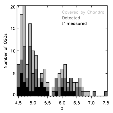
Only 54 of the 1133 $z\geq 4.5$ quasars are detected in the FIRST and/or NVSS surveys. 52 of the 54 radio detected quasars have a separation between the radio and optical positions $<3^{\prime\prime}$. 24 radio detected quasars have been covered by the Chandra observations studied in this work (Fig. 1; Table 1), and all of them have a separation between the radio and optical positions $<3^{\prime\prime}$. Following Ba$\rm\tilde{n}$ados et al. (2015), we adopt a criterion of $R\equiv L_{\rm 5GHz}/L_{\rm 4400\text{\AA}}=10$ to separate radio-loud and radio-quiet quasars, where $L_{\rm 5GHz}$ and $L_{\rm 4400\text{\AA}}$ are the rest-frame monochromatic luminosities at $5\rm~{}GHz$ and $4400\rm~{}\AA$, respectively. $L_{\rm 5GHz}$ is directly calculated from the 1.4 GHz radio flux, assuming a radio spectral index of $\alpha_{\rm R}=0.75$, while $L_{\rm 4400\text{\AA}}$ is calculated from $M_{\rm 1450\rm\text{\AA}}$, assuming a UV spectral index of $\alpha_{\rm UV}=0.5$.

Both the FIRST and NVSS surveys are relatively shallow, with a typical detection limit of $\gtrsim 1\rm~{}mJy$. They also do not cover the entire sky. Therefore, the radio properties of our $z\geq 4.5$ quasar sample are incomplete. We only use these surveys to identify some of the most radio-loud quasars. As shown in Fig. 1, most of our quasars matched to Kimball & Ivezi$\rm\acute{c}$ (2008)’s radio catalogue are highly radio-loud with $R\gtrsim 100$. Examples of deeper radio observations of high-$z$ quasars are presented in some recent works (e.g., Ba$\rm\tilde{n}$ados et al. 2015; Liu et al. 2021; Ighina et al. 2021), but the radio properties of quasars in these works are not included in our catalogue.

The X-ray luminosity of high-$z$ quasars are often computed in different ways in different literatures, which could cause significant systematic biases (e.g., Vito et al. 2019). Therefore, we reanalyze all the Chandra observations of our sample quasars, in order to ensure that their X-ray properties are derived in a uniform way.

We develop a uniform Chandra data reduction procedure for high-$z$ quasars which was partly described in Li et al. (2021) as an initial test. In the present paper, the Chandra data of all the quasars are reduced in a uniform manner with CIAO v4.12 and CALDB v4.9.2.1. The data reduction also requires some commonly used IDL packages. The scripts have not yet been tested under other versions of CIAO and CALDB, which however, should not cause serious problems. The only required input parameters of our scripts are the location (RA, DEC) of the quasar, its redshift and the $1450\rm~{}\AA$ absolute magnitude $M_{\rm 1450\text{\AA}}$. If $M_{\rm 1450\text{\AA}}$ is not given, the derived optical-to-X-ray spectral slope $\alpha_{\rm OX}$ (defined as $\alpha_{\rm OX}\equiv\frac{\log(L_{\rm 2keV}/L_{\rm 2500\text{\AA}})}{\log(\nu_{\rm 2keV}/\nu_{\rm 2500\text{\AA}})}$, where $L_{\rm 2keV}$ and $L_{\rm 2500\text{\AA}}$ are the rest-frame monochromatic luminosities at frequencies $\nu_{\rm 2keV}$ and $\nu_{\rm 2500\text{\AA}}$, respectively) will be incorrect, but the other X-ray parameters are still correct. The scripts also have quite a lot of pre-defined parameters with default values, which could be changed by the users. We summarize in Table A2 all the parameters used in these scripts.

Below we describe in detail the data reduction steps adopted in the scripts. We first search for the Chandra data covering the optical/near-IR location of a target quasar using the CIAO tool find_chandra_obsid. We utilize all the released non-grating Chandra/ACIS observations before Sep. 9th, 2020. X-ray spectral analysis will need a parameter $N_{\rm H}$, which is the foreground absorption column density mostly contributed by the Milky Way (MW). We obtain this parameter using the FTOOL nh, which is based on a few H I surveys (Dickey & Lockman, 1990; Kalberla et al., 2005; Ben Bekhti et al., 2016). In the main band of interest ($\geq 0.5\rm~{}keV$ in the observational frame, corresponding to $\gtrsim 3\rm~{}keV$ in the rest frame at $z\approx 5$), the intrinsic absorption of the quasar is typically negligible, expect for some highly obscured quasars with $N_{\rm H}>10^{22}\rm~{}cm^{-2}$. Since in most of the cases the counts number is not high enough to directly measure $N_{\rm H}$, we fix it at the MW foreground value in the following analysis. The selected Chandra data is downloaded using the CIAO tool download_chandra_obsid. We then reprocess all the raw data following the standard Chandra data reduction steps using the CIAO tool chandra_repro.

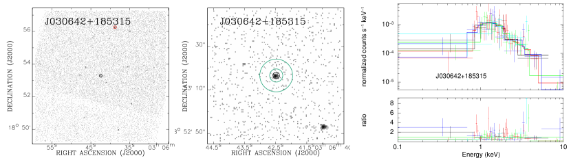
For quasars with more than one Chandra observation, we need to merge the Chandra images before further analysis. In order to align different observations, we first detect point-like sources in a $8^{\prime}\times 8^{\prime}$ box around the quasar with the CIAO tool wavdetect. We then adopt the brightest point-like source covered by all the observations as the reference source to calculate the shift between different observations. This shift has been used to update the coordinate information (use wcs_update) and reproject the event files (use reproject_events) before merging them with dmmerge. We show an example of multi-observations of a quasar in Fig. A3, where the reference source is marked with a red circle in the large field of view (FOV) image.

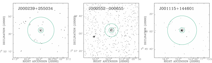
When defining the spectral analysis region (or photometry aperture), we need to determine the X-ray location of the object. We first define a $r=5^{\prime\prime}$ circular region centered at the optical/near-IR location of the quasar. We then calculate the centroid position of the broad-band (0.5-7 keV) Chandra image. This centroid position is used as the center of a new source region with a smaller radius. We then repeat the above steps and finally adopt the centroid position within a $r=2^{\prime\prime}$ circular region as the X-ray location of the quasar. If there are too few X-ray photons detected, the X-ray centroid position will be poorly determined. Therefore, when the departure of the X-ray location from the original optical/near-IR location is too large ($>3^{\prime\prime}$), we will set the location of the quasar back to the original position. We adopt a $r=1.5^{\prime\prime}$ circular region centered at the X-ray location of the quasar as the spectral analysis region or the photometry aperture. We also define an annulus centered at the X-ray location of the quasar as the background region. We first perform X-ray point source detection using the CIAO tool wavdetect, and remove all the detected point sources from the background region. The inner radius of the annulus ($r=3^{\prime\prime}$) equals to twice of the radius of the source region ($r=1.5^{\prime\prime}$), while the outer radius is initially set to $r=7.5^{\prime\prime}$. The outer radius is further enlarged step by step to a maximum value of 10 times of the radius of the source region, until the total number of background counts is $\geq 10$. If the total number of background counts is still $<10$ after the outer radius reaches the maximum value, we add a label “c” in front of the name of the quasar and plot it with a different symbol in the following analysis. Examples of source and background regions of a few quasars are presented in Figs. A1 and A3.

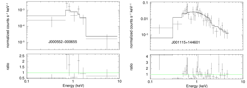
We extract a spectrum of each observation of a quasar using the CIAO tool specextract. Sometimes when there are too few counts, there will be no spectrum extracted for a certain observation. The spectra from different observations are jointly analyzed using an absorbed redshifted power law model, with the foreground absorption column density fixed at the MW value and the redshift fixed at that obtained from the optical/near-IR spectroscopy. The only free parameters are the X-ray flux and photon index $\Gamma$. Typically a spectral analysis with a simple power law model is only reliable if the net background-subtracted counts number is $\geq 20$. Nevertheless, we also conduct spectral analysis for all the quasars with a net counts number $=10-20$, which are just used for comparison. The spectral analysis results of these quasars will not be included in the online table or in the scientific discussions below, but a figure of the spectrum is put online so the readers can double check. For quasars with a net counts number $<20$, we directly calculate the X-ray flux based on the net counts rate in 0.5-2 keV and a constant counts rate to flux conversion factor obtained assuming an absorbed power law model with $N_{\rm H}=5\times 10^{20}\rm~{}cm^{-2}$, $\Gamma=2.0$, and $z=6.0$. Small changes of the these parameters do not significantly affect the results. We adopt the on-axis response files to calculate this conversion factor, which will slightly under-estimate the flux of objects at large off-axis distances. We include the original counts number and effective Chandra exposure time in the online catalogue, so users could calculate the X-ray flux in different bands using their own models. We also assume $\Gamma=2.0$ for all these quasars when converting the flux and luminosity in different bands. When calculating $\alpha_{\rm OX}$ using the measured X-ray luminosity and $M_{\rm 1450\text{\AA}}$, we assume the same UV spectral index ($\alpha_{\rm UV}=0.5$) and bolometric correction factor ($\rm BC_{3000}=5.15$ at $3000\rm~{}\text{\AA}$) as above (§2.1).

In our online catalogue, we do not set a fixed detection criterion. Instead, we list the 1 $\sigma$ rms of the background counts rate in different bands and the 1 $\sigma$ measurement errors of the X-ray flux and luminosity (Table A1). Therefore, users could define their own detection significance as needed using these parameters. As an example, we present a summary of the X-ray detection rate of the quasars and the redshift distribution of the sample in Fig. 2, where the detection of an X-ray source is at $>1\rm~{}\sigma$ confidence level in 0.5-2 keV in the observational frame. Under this criterion, we detect 91 of the 152 quasars in the sample (Table 1). However, in the remaining part of this paper, we plot the X-ray fluxes and luminosities as well as their upper limits all at 3 $\sigma$ confidence level. Only 46 quasars have been firmly detected above this level (Table 1). We are also able to estimate the power law photon index $\Gamma$ of the X-ray spectrum of 31 quasars (Table 1), but the error of $\Gamma$ is quoted at 1 $\sigma$ confidence level which is consistent with the original definition in the spectral analysis and could not be directly converted to the 3 $\sigma$ error. The measured X-ray fluxes of the quasars are also summarized in Fig. 3. As our sample quasars are not observed in a uniform way, the measured flux detection limit of non-detected sources does not show a tight correlation with the effective Chandra exposure time.

In addition to the parameters from the Chandra observations, we also checked the available XMM-Newton data of the sample quasars and listed them in the data table. Analyzing the XMM-Newton data, however, is beyond the scope of the present paper. If interested in these data, we suggest the readers to check a few systematic studies of the X-ray properties of high-$z$ quasars largely based on the XMM-Newton data (e.g., Lusso & Risaliti 2016; Lusso et al. 2020; Salvestrini et al. 2019; Pons et al. 2020). Basic information of these XMM-Newton observations, together with the optical/near-IR/radio properties, as well as the X-ray properties of the quasars measured in this work, are all listed in the data table, which has been put online in FITS format. Furthermore, we also add some special notes on some quasars in the online table, such as identified blazars and broad absorption line (BAL) quasars. However, as these identifications are not uniformly conducted for all the sample quasars, we do not list them as separated parameters nor use them in the following statistical analysis. A brief description of different columns of this online catalogue is summarized in the appendix (Table A1).

We first compare the rest frame 2-10 keV luminosity $L_{\rm 2-10keV}$ to the bolometric luminosity ($L_{\rm bol}$) and SMBH mass ($M_{\rm SMBH}$) of the quasars (Fig. 4). As $M_{\rm SMBH}$ is only known for a small fraction of the quasars, we do not include other samples on our $L_{\rm 2-10keV}-M_{\rm SMBH}$ plot (Fig. 4b).

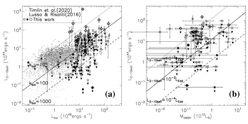
Emission in the X-ray band is typically less important than in the UV band in the AGN bolometric luminosity, but is closely related to the central engine of the AGN. A positive $L_{\rm 2-10keV}-L_{\rm bol}$ correlation (or more generally the $L_{\rm X}-L_{\rm UV}$ correlation as will be discussed in §3.2) is often suggested in previous works (e.g., Risaliti & Lusso 2015), as also indicated by the data points from Lusso & Risaliti (2016); Timlin et al. (2020) in Fig. 4a. Most of our sample quasars with low $L_{\rm 2-10keV}$ (e.g., $L_{\rm 2-10keV}\lesssim 10^{45}\rm~{}ergs~{}s^{-1}$) are upper limits, which show a large scatter on the $L_{\rm 2-10keV}-L_{\rm bol}$ plot. We also found most of the confirmed extremely radio-loud quasars appear to be very X-ray bright. If we remove these radio-loud quasars and the upper limits, the other firmly detected quasars in X-ray are roughly consistent with quasars at lower redshifts. Compared to other works, the apparently larger scatter on $L_{\rm 2-10keV}$ of our $z\geq 4.5$ quasars could be at least partially attributed to the poorly X-ray data (upper limit of many X-ray faint quasars) and the radio-loudness. We find most of the quasars have an X-ray bolometric correction factor ($k_{\rm bol}\equiv L_{\rm bol}/L_{\rm 2-10keV}$) in the range of $k_{\rm bol}=10-1000$ found by Wang et al. (2021) for their $z>6.5$ quasar sample, except for some extremely radio-loud quasars and many X-ray non-detected quasars where the determination of the upper limits are affected by the data quality and the applied criteria. $k_{\rm bol}$ may be systematically higher at larger $L_{\rm bol}$, indicating that more luminous quasars tend to be relatively X-ray fainter, but still follow a continuous trend connecting less luminous quasars. This is also consistent with their steeper optical-to-X-ray spectral slope (smaller $\alpha_{\rm OX}$), as will be discussed in §3.3.

We also compare $L_{\rm 2-10keV}$ to $M_{\rm SMBH}$ and the Eddington ratio $\lambda_{\rm Edd}$ in Fig. 4b. As $M_{\rm SMBH}$ and $\lambda_{\rm Edd}$ are not available for most samples and many of our sample quasars, we only plot 76 quasars from our sample in Fig. 4b. We do not see any significant correlation between $L_{\rm 2-10keV}$ and $M_{\rm SMBH}$. The X-ray emission is typically in the range of $\sim 10^{-(2-4)}L_{\rm Edd}$, which is small compared to the emission in the UV band. A similar conclusion has also been obtained in previous works (e.g., Martocchia et al. 2017). The X-ray weakness of these hyper-luminous quasars compared to less luminous AGNs could be partially attributed to the perturbation of the disk corona by powerful radiation driven winds as often indicated by the blueshifted high-ionization UV lines in their spectra (see discussions on various explanations of the X-ray weakness in Proga 2005; Martocchia et al. 2017 and references therein).

The relation between the X-ray and UV emissions is one of the tightest correlations of the X-ray properties of AGN (e.g., Lusso & Risaliti 2016, 2017; Risaliti & Lusso 2019). The relation is often expressed in different ways, with the X-ray and UV emissions expressed in monochromatic or broad-band flux or luminosity, or $\alpha_{\rm OX}$, etc. (e.g., Just et al. 2007; Martocchia et al. 2017; Vito et al. 2019; Timlin et al. 2020). The $L_{\rm X}-L_{\rm UV}$ relation is significantly non-linear, but its slope shows no significant redshift evolution based on existing observations (e.g., Risaliti & Lusso 2015; Salvestrini et al. 2019). We will discuss the $\alpha_{\rm OX}-L_{\rm UV}$ relation in §3.3 and the implication of the X-ray-UV relations as the standard candle in cosmology in §3.5. In this section, we focus on comparing the slope of the $L_{\rm X}-L_{\rm UV}$ relation in different AGN samples.

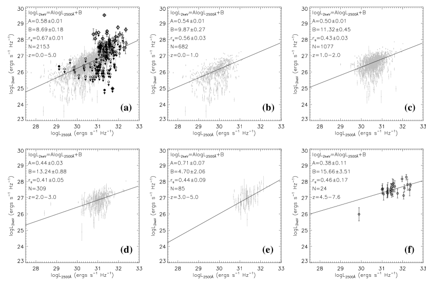
In Fig. 5, we present the X-ray-UV correlation of AGN in the form of the $L_{\rm 2keV}-L_{\rm 2500\text{\AA}}$ relationship, where $L_{\rm 2keV}$ and $L_{\rm 2500\text{\AA}}$ are the monochromatic luminosities of the AGN at $2\rm~{}keV$ and $2500\rm~{}\text{\AA}$, derived from the measured 0.5-2 keV flux and $1450\rm~{}\text{\AA}$ magnitude, respectively. We divide Lusso & Risaliti (2016)’s sample into four different redshift bins at $z<5$ and compare them to our own sample at the highest redshift bin at $z\geq 4.5$. We adopt the Spearman’s rank order correlation coefficient ($r_{\rm s}$) to quantify the tightness of the correlation. We consider $|r_{\rm s}|\gtrsim 0.6$ or $0.3\lesssim|r_{\rm s}|\lesssim 0.6$ as a tight or weak correlation, and $|r_{\rm s}|\lesssim 0.3$ as no correlation (e.g., Li & Wang 2013). We only used the firm detections from Lusso & Risaliti (2016) in the plots. Similarly, upper limits and confirmed extremely radio-loud quasars from our own sample are also removed when fitting the relation and calculating $r_{\rm s}$.

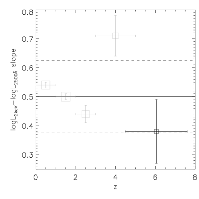
There is a tight correlation between $L_{\rm 2keV}$ and $L_{\rm 2500\text{\AA}}$ for the whole sample from Lusso & Risaliti (2016) ($r_{\rm s}\approx 0.67$), and our $z\geq 4.5$ quasar sample also appear to be roughly consistent with the overall trend (Fig. 5a). However, when we divide the sample into different redshift bins, the correlation becomes much weaker, largely because of the much narrower $L_{\rm 2keV}$ or $L_{\rm 2500\text{\AA}}$ ranges (Fig. 5b-e). We show in Fig. 6 the redshift evolution of the measured slope of the $L_{\rm 2keV}-L_{\rm 2500\text{\AA}}$ relation. The scatter is quite large, especially at high redshifts. Therefore, although the measured slope at $z=3-5$ from Lusso & Risaliti (2016)’s sample appears to be steeper than those at other redshifts, we do not think there is significant evidence for a redshift evolution of the X-ray-UV relation based on the existing data. This is also claimed in previous studies (e.g., Risaliti & Lusso 2015; Salvestrini et al. 2019). The median value of the $\log L_{\rm 2keV}-\log L_{\rm 2500\text{\AA}}$ slope is $0.50\pm 0.13$, which is significantly sub-linear.

The optical-to-X-ray spectral slope $\alpha_{\rm OX}$ is a redshift independent parameter and a good tracer of the relative importance of the accretion disk vs corona emission from the AGN (e.g., Brandt & Alexander 2015). In this section, we compare our sample to the well defined scaling relation between $\alpha_{\rm OX}$ and $L_{\rm UV}$ (expressed in the monochromatic luminosity $L_{\rm 2500\text{\AA}}$; Fig. 7a). It is clear that both the data and the best-fit $\alpha_{\rm OX}-L_{\rm 2500\text{\AA}}$ relations from different works have large scatter (e.g., Just et al. 2007; Nanni et al. 2017; Martocchia et al. 2017; Timlin et al. 2020). Our sample of $z\geq 4.5$ quasars is roughly consistent with all the $\alpha_{\rm OX}-L_{\rm 2500\text{\AA}}$ relations from previous works and fills the gap at the high end of $L_{\rm 2500\text{\AA}}$. The apparent large scatter of our high-$z$ quasars on the $\alpha_{\rm OX}-L_{\rm 2500\text{\AA}}$ relation is again caused by the poor X-ray data (upper limits) and the radio-loud quasars.

We investigate the redshift evolution of the $\alpha_{\rm OX}-L_{\rm 2500\text{\AA}}$ relation by calculating the departure of the data points from Timlin et al. (2020)’s relation ($\Delta\alpha_{\rm OX}$) at different redshifts (Fig. 7b). Similar as found by the other authors (e.g., Just et al. 2007; Vito et al. 2019; Wang et al. 2021), we do not find any significant redshift evolution of $\Delta\alpha_{\rm OX}$. The slight systematic increase of $\Delta\alpha_{\rm OX}$ with redshift for Lusso & Risaliti (2016)’s sample is caused by their different $\alpha_{\rm OX}-L_{\rm 2500\text{\AA}}$ slopes which may be a result of the sample selection bias to more luminous AGN at higher redshifts, instead of a true redshift evolution.

We further study the dependence of the scatter of our $z\geq 4.5$ quasar sample on other AGN parameters in Fig. 8. We quantify the scatter by calculating the departure of the measured $\alpha_{\rm OX}$ from the best-fit $\alpha_{\rm OX}-L_{\rm 2500\text{\AA}}$ relationships from Just et al. (2007); Nanni et al. (2017); Martocchia et al. (2017); Timlin et al. (2020) as plotted in Fig. 7a. Upper limits on $\alpha_{\rm OX}$ have been removed from both the fitting and the plot. The confirmed radio-loud quasars have also been removed from the fitting but are still plotted on the figure for comparison. We do not find a strong dependence of $\Delta\alpha_{\rm OX}$ on some other quasar parameters such as the $M_{\rm SMBH}$ or $\lambda_{\rm Edd}$, as also suggested in some previous works (e.g., Vito et al. 2018b). However, we find a strong dependence of $\Delta\alpha_{\rm OX}$ on the X-ray luminosity of the quasar ($L_{\rm 2-10keV}$ or $L_{\rm 2keV}$; the $\Delta\alpha_{\rm OX}-L_{\rm 2keV}$ relation is presented in Fig. 8). The tight correlation between $\Delta\alpha_{\rm OX}$ and $L_{\rm 2keV}$ of our sample (after excluding the upper limits and confirmed radio-loud quasars; $r_{\rm s}\sim 0.6$), as well as the significant difference between our sample and Lusso & Risaliti (2016); Timlin et al. (2020)’s samples at lower redshifts, suggest that the $L_{\rm X}-L_{\rm UV}$ relation of these samples at different redshift ranges and with different X-ray luminosities may have different slopes.

We would like to emphasize that the tight correlation between $\Delta\alpha_{\rm OX}$ and $L_{\rm 2keV}$ as presented in Fig. 8 is not a new physical relation. As $\alpha_{\rm OX}$ is defined as $\frac{\log(L_{\rm 2keV}/L_{\rm 2500\text{\AA}})}{\log(\nu_{\rm 2keV}/\nu_{\rm 2500\text{\AA}})}$, the $\Delta\alpha_{\rm OX}-L_{\rm 2keV}$ relation could be merged into the $\alpha_{\rm OX}-L_{\rm 2500\text{\AA}}$ relation. The tight $\Delta\alpha_{\rm OX}-L_{\rm 2keV}$ correlation simply means the slope of the $\alpha_{\rm OX}-L_{\rm 2500\text{\AA}}$ relation for our $z\geq 4.5$ quasar sample is clearly different from those defined with other AGN samples. As the $L_{\rm 2500\text{\AA}}$ and $L_{\rm 2keV}$ ranges of the high-$z$ quasar sample do not extend to the low luminosity end, the slope of the $\alpha_{\rm OX}-L_{\rm 2500\text{\AA}}$ relation cannot be well constrained. We therefore do not fit a separated $\alpha_{\rm OX}-L_{\rm 2500\text{\AA}}$ relation for our high-$z$ quasar sample. From Fig. 8, we also notice that at least part of the scatter could be attributed to the inclusion of the radio-loud quasars in the sample. We have not identified all the radio-loud quasars, and there are some other types of quasars whose observed X-ray properties may be significantly biased (e.g., blazars and BALs which are included in the “NOTE” of the online table). Therefore, the different slopes of the $\alpha_{\rm OX}-L_{\rm 2500\text{\AA}}$ relation of our sample and other samples may be at least partially attributed to the sample selection bias. Our data do not indicate a clear difference in the $\alpha_{\rm OX}-L_{\rm 2500\text{\AA}}$ slope of high-$z$ quasars.

The X-ray spectral slope, often expressed with the photon index of a power law fit to the hard X-ray spectrum ($\Gamma$), is thought to be closely related to the accretion rate of the SMBH which is often expressed with the Eddington ratio $\lambda_{\rm Edd}$ (e.g., Nowak 1995). At higher accretion rates, the enhanced emission from the accretion disk could provide more UV photons to cool the disk corona via inverse Compton emission, resulting in a lower corona temperature and a steeper X-ray spectrum (larger $\Gamma$). Such a $\Gamma-\lambda_{\rm Edd}$ correlation has been suggested in previous works (e.g., Shemmer et al. 2006, 2008; Brightman et al. 2013; however, see report of a much weaker correlation in Trakhtenbrot et al. 2017), which is especially important as an independent measurement of the SMBH growth history in X-ray band.

In Fig. 9a, we compare the measured $\Gamma$ of our sample to other AGN samples at different redshifts (Lusso & Risaliti, 2016; Timlin et al., 2020; Wang et al., 2021). The median value of $\Gamma$ of our $z\geq 4.5$ quasars is $1.79\pm 0.57$ (plotted as solid and dashed lines in Fig. 9a). It is clear that within the uncertainties, we do not see any significant redshift evolution of the accretion activity as traced by $\Gamma$. This is consistent with what has been found in previous works (e.g., Just et al. 2007; Vito et al. 2019; Wang et al. 2021). The data point at the highest redshift bin ($z>6.5$) is based on a stacked X-ray spectrum instead of measurements of individual quasars (Wang et al., 2021). The slightly higher $\Gamma$ may not be representative as the average $\lambda_{\rm Edd}$ is also high. We plot this data point, as well as quasars from our sample with both $\Gamma$ and $\lambda_{\rm Edd}$ measured, on the $\Gamma-\lambda_{\rm Edd}$ relation (Fig. 9b). We also plot in Fig. 9b the best-fit $\Gamma-\lambda_{\rm Edd}$ relation from Brightman et al. (2013) for comparison. Brightman et al. (2013)’s sample has a $\lambda_{\rm Edd}$ range of $\log\lambda_{\rm Edd}\approx(-2.5-0)$, so the data plotted in Fig. 9b represent the high end of this relation. This plot confirms that the apparently higher $\Gamma$ of the highest-redshift quasars is indeed caused by their larger $\lambda_{\rm Edd}$, which is a sample selection effect instead of a real redshift evolution.

Based on their high multi-band luminosity and the well-defined UV-X-ray scaling relations (often expressed in the $\alpha_{\rm OX}-L_{\rm 2500\text{\AA}}$ relation; see §3.3), quasars could potentially be adopted as a standard candle in a broad redshift range to constrain cosmological models (e.g., Risaliti & Lusso 2015, 2019; Lusso & Risaliti 2017; Lusso et al. 2020). In this section, we compare our $z\geq 4.5$ quasars to the latest combined quasar sample from Lusso et al. (2020) on the Hubble diagram (distance modulus vs redshift; Fig. 10). 19 of the 152 quasars included in our sample are also included in Lusso et al. (2020)’s sample. The overlap of the two samples will not significantly affect the comparison and the discussions in this section. Also plotted in Fig. 10a is the cosmological model adopted in the present paper (§1). We do not fit a cosmological model as the scatter of the data is too large to well constrain it.

As discussed in previous sections, the physical foundation of adopting the UV and X-ray properties of AGN as a standard candle is the physical link between the accretion disk and corona of a SMBH. We expect higher accretion rate will produce stronger UV emission from the accretion disk (higher $L_{\rm 2500\text{\AA}}$), while more efficient cooling of the corona via inverse Compton emission, so softer X-ray emission or lower X-ray-to-UV flux ratio (lower $\alpha_{\rm OX}$). As the flux ratio $\alpha_{\rm OX}$ is directly measurable and redshift independent, we can use it and the $\alpha_{\rm OX}-L_{\rm 2500\text{\AA}}$ relation to estimate $L_{\rm 2500\text{\AA}}$. Combined with the measured flux or magnitude at the rest-frame UV band, we can estimate the distance modulus and compare it to the measured redshift on the Hubble diagram.

The reliability of the above method depends on the tightness and redshift dependence of the $\alpha_{\rm OX}-L_{\rm 2500\text{\AA}}$ relation. As discussed in §3.3, the $\alpha_{\rm OX}-L_{\rm 2500\text{\AA}}$ relation shows significant scatter, especially for our high-$z$ quasar sample which often has poor X-ray data and is a mixture of radio-loud and radio-quiet quasars. However, we do not find significant evidence for a clear redshift evolution of the UV-X-ray relation (§3.2), although this argument is far from conclusive due to the strong bias in the largely flux limited sample selection at different redshifts. Therefore, the overall conclusion is that we can use the UV and X-ray properties of quasars as a standard candle, but the scatter will be extremely large, which comes from both the measurement error and the uncertainty of the $\alpha_{\rm OX}-L_{\rm 2500\text{\AA}}$ relation (error bars of individual data points are not plotted in Fig. 10). As our sample represents quasars detected in X-ray at the highest redshifts, it plays a potentially critical role in constraining the cosmological models.

As shown in Fig. 10a, our $z\geq 4.5$ quasars are roughly consistent with quasars at lower redshifts. They however put little constraint on different cosmological models due to the large scatter and the measurement error. The median value of the distance modulus of our $z\geq 4.5$ quasars may sit below the cosmological model adopted in this paper (the dashed curve). This is partially because the model is not a fitted relation to the data. However, the systematic bias from Lusso et al. (2020)’s sample (all radio quiet) in the same redshift range may be largely caused by the inclusion of radio-loud quasars. As the FIRST and NVSS surveys adopted in the present paper are only sensitive to quasars with $R\gtrsim 100$ (Fig. 1), there may still be some radio-loud quasars not yet identified which have lowered the median value of the distance modulus. As the jet could contribute significantly to both the observed radio and X-ray emissions in radio-loud quasars, especially in blazars (e.g., Romani et al. 2006; An & Romani 2018; Ighina et al. 2021), these objects do not follow the $\alpha_{\rm OX}-L_{\rm 2500\text{\AA}}$ relation and should be removed when comparing to different cosmological models.

As we found a strong dependence of the departure of $\alpha_{\rm OX}$ from the best-fit $\alpha_{\rm OX}-L_{\rm 2500\text{\AA}}$ relation ($\Delta\alpha_{\rm OX}$) on the monochromatic X-ray luminosity ($L_{\rm 2keV}$; Fig. 8), we use this relation to correct the $\alpha_{\rm OX}-L_{\rm 2500\text{\AA}}$ relation for our $z\geq 4.5$ quasars and recalculate the distance modulus. To do this, we first calculate $\Delta\alpha_{\rm OX}$ with the measured $L_{\rm 2keV}$ and the best-fit $\Delta\alpha_{\rm OX}-L_{\rm 2keV}$ relation in Fig. 8d. We then add this derived $\Delta\alpha_{\rm OX}$ back to the measured $\alpha_{\rm OX}$, use this new $\alpha_{\rm OX}$ and Timlin et al. (2020)’s $\alpha_{\rm OX}-L_{\rm 2500\text{\AA}}$ relation to calculate a predicted $L_{\rm 2500\text{\AA}}$. We further calculate the corrected distance modulus using this predicted $L_{\rm 2500\text{\AA}}$ and the measured monochromatic flux at rest-frame $2500\rm~{}\text{\AA}$. The results are shown in Fig. 10b, with a clearly smaller scatter on the distance modulus. However, as already being pointed out in §3.3, the $\Delta\alpha_{\rm OX}-L_{\rm 2keV}$ relation is not a real physical relation, but indeed caused by the poor determination of the $\alpha_{\rm OX}-L_{\rm 2500\text{\AA}}$ relation for the highest redshift quasars. Therefore, the above calculation of the corrected distance modulus in Fig. 10b is just used to show the potential of a better determination of the $\alpha_{\rm OX}-L_{\rm 2500\text{\AA}}$ slope to better constrain the cosmological model. It should not be adopted as a standard method to reduce the scatter on the Hubble diagram. Future unbiased X-ray and radio surveys of high-$z$ quasars with lower detection limits could help to well constrain the $\alpha_{\rm OX}-L_{\rm 2500\text{\AA}}$ relation for radio-quiet quasars in a broad luminosity range, thus help to make use of AGNs as a standard candle for cosmological studies.

References

- An & Romani (2018) An H., Romani R. W., 2018, ApJ, 856, 105
- Baados et al. (2015) Baados E., Venemans B. P., Morganson E., Hodge J., Decarli R., et al., 2015, ApJ, 804, 118
- Baados et al. (2016) Baados E., Venemans B. P., Decarli R., Farina E. P., Mazzucchelli C., et al., 2016, ApJS, 227, 11
- Baados et al. (2018) Baados E., Connor T., Stern D., Mulchaey J., Fan X., et al., 2018, ApJL, 856, 25
- Ben Bekhti et al. (2016) Ben Bekhti N., Fler L., Keller R., Kerp J., Lenz D., et al., 2016, A&A, 594, 116
- Brandt & Alexander (2015) Brandt W. N., Alexander D. M., 2015, A&A Rv, 23, 1
- Brightman et al. (2013) Brightman M., Silverman J. D., Mainieri V., Ueda Y., Schramm M., et al., 2013, MNRAS, 433, 2485
- Coatman et al. (2017) Coatman L., Hewett P. C., Banerji M., Richards G. T., Hennawi J. F., Prochaska J. X., 2017, MNRAS, 465, 2120
- De Rosa et al. (2011) De Rosa G., Decarli R., Walter F., Fan X., Jiang L., Kurk J., Pasquali A., Rix H. W., 2011, ApJ, 739, 56
- Dickey & Lockman (1990) Dickey J. M., Lockman F. J., 1990, ARA&A, 28, 215
- Fabian (2006) Fabian A. C., 2006, AN, 327, 943
- Fabian (2012) Fabian A. C., 2012, ARA&A, 50, 455
- Fan et al. (2019) Fan X., Wang F., Yang J., Keeton C. R., Yue M., et al., 2019, ApJ, 870, 11
- Ighina et al. (2021) Ighina L., Belladitta S., Caccianiga A., Broderick J. W., Drouart G., Moretti A., Seymour N., 2021, A&AL, 647, 11
- Jun et al. (2015) Jun H. D., Im M., Lee H. M., Ohyama Y., Woo J.-H., et al., 2015, ApJ, 806, 109
- Just et al. (2007) Just D. W., Brandt W. N., Shemmer O., Steffen A. T., Schneider D. P., Chartas G., Garmire G. P., 2007, ApJ, 665, 1004
- Kalberla et al. (2005) Kalberla P. M. W., Burton W. B., Hartmann D., Arnal E. M., Bajaja E., et al., 2005, A&A, 440, 775
- Kelly et al. (2008) Kelly B. C., Bechtold J., Trump J. R., Vestergaard M., Siemiginowska A., 2008, ApJS, 176, 355
- Kim & Im (2019) Kim Y., Im M., 2019, ApJ, 879, 117
- Kimball & Ivezi (2008) Kimball A. E., Ivezi ., 2008, AJ, 136, 684
- Li & Wang (2013) Li J.-T., Wang Q. D., 2013, MNRAS, 435, 3071
- Li et al. (2021) Li J.-T., Wang F., Yang J., Zhang Y., Fu Y., et al., 2021, ApJ, 906, 135.
- Liu et al. (2021) Liu Y., Wang R., Momjian E., Banados E., Zeimann G., et al., 2021, ApJ, 908, 124
- Luo et al. (2014) Luo B., Brandt W. N., Alexander D. M., Stern D., Teng S. H., et al., 2014, ApJ, 794, 70
- Lusso & Risaliti (2016) Lusso E., Risaliti G., 2016, ApJ, 819, 154
- Lusso & Risaliti (2017) Lusso E., Risaliti G., 2017, A&A, 602, 79
- Lusso et al. (2020) Lusso E., Risaliti G., Nardini E., Bargiacchi G., Benetti M., et al., 2020, A&A, 642, 150
- Martocchia et al. (2017) Martocchia S., Piconcelli E., Zappacosta L., Duras F., Vietri G., et al., 2017, A&A, 608, 51
- Matsuoka et al. (2019) Matsuoka Y., Onoue M., Kashikawa N., Strauss M. A., Iwasawa K., et al. 2019, ApJL, 872, 2
- Mazzucchelli et al. (2017) Mazzucchelli C., Baados E., Venemans B. P., Decarli R., Farina E. P., et al., 2017, ApJ, 849, 91
- Medvedev et al. (2020) Medvedev P., Sazonov S., Gilfanov M., Burenin R., Khorunzhev G., et al., 2020, MNRAS, 497, 1842
- Moretti et al. (2014) Moretti A., Ballo L., Braito V., Caccianiga A., Della Ceca R., et al., 2014, A&A, 563, 46
- Mushotzky et al. (1993) Mushotzky R. F., Done C., Pounds K. A., 1993, ARA&A, 31, 717
- Nanni et al. (2017) Nanni R., Vignali C., Gilli R., Moretti A., Brandt W. N., 2017, A&A, 603, 128
- Netzer et al. (2014) Netzer H., Mor R., Trakhtenbrot B., Shemmer O., Lira P., 2014, ApJ, 791, 34
- Nowak (1995) Nowak M. A., 1995, PASP, 107, 1207
- Onoue et al. (2019) Onoue M., Kashikawa N., Matsuoka Y., Kato N., Izumi T., et al., 2019, ApJ, 880, 77
- Page et al. (2014) Page M. J., Simpson C., Mortlock D. J., Warren S. J., Hewett P. C., Venemans B. P., McMahon R. G., 2014, MNRASL, 440, 91
- Proga (2005) Proga D., 2005, ApJL, 630, 9
- Pons et al. (2020) Pons E., McMahon R. G., Banerji M., Reed S. L., 2020, MNRAS, 491, 3884
- Porquet et al. (2004) Porquet D., Reeves J. N., O’Brien P., Brinkmann W., 2004, A&A, 422, 85
- Reed et al. (2019) Reed S. L., Banerji M., Becker G. D., Hewett P. C., Martini P., et al., 2019, MNRAS, 487, 1874
- Risaliti & Lusso (2015) Risaliti G., Lusso E., 2015, ApJ, 815, 33
- Risaliti & Lusso (2019) Risaliti G., Lusso E., 2019, Nature Astronomy, 3, 272
- Romani et al. (2006) Romani R. W., 2006, AJ, 132, 1959
- Salvestrini et al. (2019) Salvestrini F., Risaliti G., Bisogni S., Lusso E., Vignali C., 2019, A&A, 631, 120
- Schindler et al. (2020) Schindler J.-T., Farina E. P., Baados E., Eilers A.-C., Hennawi J. F., et al., 2020, ApJ, 905, 51
- Schulze et al. (2018) Schulze A., Silverman J. D., Kashino D., Akiyama M., Schramm M., 2018, ApJS, 239, 22
- Shemmer et al. (2006) Shemmer O., Brandt W. N., Netzer H., Maiolino R., Kaspi S., 2006, ApJL, 646, 29
- Shemmer et al. (2008) Shemmer O., Brandt W. N., Netzer H., Maiolino R., Kaspi S., 2008, ApJ, 682, 81
- Shen et al. (2011) Shen Y., Richards G. T., Strauss M. A., Hall P. B., Schneider D. P., et al., 2011, ApJS, 194, 45
- Shen et al. (2019) Shen Y., Wu J., Jiang L., Baados E., Fan X., et al., 2019, ApJ, 873, 35
- Tang et al. (2019) Tang J.-J., Goto T., Ohyama Y., Jin C., Done C., et al., 2019, MNRAS, 484, 2575
- Timlin et al. (2020) Timlin J. D., Brandt W. N., Ni Q., Luo B., Pu X., et al., 2020, MNRAS, 492, 719
- Trakhtenbrot et al. (2011) Trakhtenbrot B., Netzer H., Lira P., Shemmer O., 2011, ApJ, 730, 7
- Trakhtenbrot et al. (2017) Trakhtenbrot B., Ricci C., Koss M. J., Schawinski K., Mushotzky R., et al., 2017, MNRAS, 470, 800
- Turner & Miller (2009) Turner T. J., Miller L., 2009, A&A Rev, 17, 47
- Vestergaard & Osmer (2009) Vestergaard M., Osmer P. S., 2009, ApJ, 699, 800
- Vito et al. (2018a) Vito F., Brandt W. N., Yang G., Gilli R., Luo B., et al., 2018a, MNRAS, 473, 2378
- Vito et al. (2018b) Vito F., Brandt W. N., Luo B., Shemmer O., Vignali C., Gilli R., 2018b, MNRAS, 479, 5335
- Vito et al. (2019) Vito F., Brandt W. N., Bauer F. E., Calura F., Gilli R., et al., 2019, A&A, 630, 118
- Wang et al. (2015) Wang F., Wu X.-B., Fan X., Yang J., Cai Z., et al., 2015, ApJL, 807, 9
- Wang et al. (2016) Wang F., Wu X.-B., Fan X., Yang J., Yi W., et al., 2016, ApJ, 819, 24
- Wang et al. (2017) Wang, F., Fan, X., Yang, J., Wu, X.-B., Yang, Q., et al., 2017, ApJ, 839, 27
- Wang et al. (2018) Wang F., Yang J., Fan X., Yue M., Wu X.-B., et al., 2018, ApJL, 869, 9
- Wang et al. (2019) Wang F., Yang J., Fan X., Wu X.-B., Yue M., et al., 2019, ApJ, 884, 30
- Wang et al. (2021) Wang F., Fan X., Yang J., Mazzucchelli C., Wu X.-B., et al., 2021, ApJ, 908, 53.
- Wolf et al. (2021) Wolf J., Nandra K., Salvato M., Liu T., Buchner J., et al., 2021, A&A, 647, 5
- Worrall (2009) Worrall D. M., 2009, A&A Rev, 17, 1
- Wu et al. (2012) Wu X.-B., Zuo W.-W., Yang Q., Yi W.-M., Yang C.-W., et al., 2012, RAA, 12, 1185
- Wu et al. (2015) Wu X.-B., Wang F., Fan X., Yi W., Zuo W., et al., 2015, Nature, 518, 512
- Yang et al. (2016) Yang J., Wang F., Wu X.-B., Fan X., McGreer I. D., et al., 2016, ApJ, 829, 33
- Yang et al. (2017) Yang J., Fan X., Wu X.-B., Wang F., Bian F., et al., 2017, AJ, 153, 184
- Yang et al. (2019a) Yang J., Wang F., Fan X., Wu X.-B., Bian F., et al., 2019a, ApJ, 871, 199
- Yang et al. (2019b) Yang J., Wang F., Fan X., Yue M., Wu X.-B., et al., 2019b, AJ, 157, 236
- Yang et al. (2020) Yang J., Wang F., Fan X., Hennawi J. F., Davies F. B., et al., 2020, ApJL, 897, 14
- Yi et al. (2014) Yi W.-M., Wang F., Wu X.-B., Yang J., Bai J.-M., et al., 2014, ApJL, 795, 29
- Yu et al. (2021) Yu X., Li J.-T., Qu Z., Roederer I. U., Bregman J. N., et al., 2021, submitted
Appendix A Online Materials: Data Table, Chandra Images and Spectra
We present some examples of the Chandra images and spectra of our sample quasars in this section. Similar figures of all the quasars, as well as our scripts for the pipeline data reduction, are available as the online only data. All the figures presented in this section are generated automatically with the pipeline.