A change of measure preserving the affine structure in the BNS model for commodity markets
Abstract.
For a commodity spot price dynamics given by an Ornstein-Uhlenbeck process with Barndorff-Nielsen and Shephard stochastic volatility, we price forwards using a class of pricing measures that simultaneously allow for change of level and speed in the mean reversion of both the price and the volatility. The risk premium is derived in the case of arithmetic and geometric spot price processes, and it is demonstrated that we can provide flexible shapes that is typically observed in energy markets. In particular, our pricing measure preserves the affine model structure and decomposes into a price and volatility risk premium, and in the geometric spot price model we need to resort to a detailed analysis of a system of Riccati equations, for which we show existence and uniqueness of solution and asymptotic properties that explains the possible risk premium profiles. Among the typical shapes, the risk premium allows for a stochastic change of sign, and can attain positive values in the short end of the forward market and negative in the long end.
1. Introduction
Benth and Ortiz-Latorre [9] analysed a structure preserving class of pricing measures for Ornstein-Uhlenbeck (OU) processes with applications to forward pricing in commodity markets. In particular, they considered multi-factor OU models driven by Lévy processes having positive jumps (so-called subordinators) or Brownian motions for the spot price dynamics and analysed the risk premium when the level and speed of mean reversion in these factor processes were changed.
In this paper we continue this study for OU processes driven by Brownian motion, but with a stochastic volatility perturbing the driving noise. The stochastic volatility process is modelled again as an OU process, but driven by a subordinator. This class of stochastic volatility models were first introduced by Barndorff-Nielsen and Shephard [1] for equity prices, and later analysed by Benth [2] in commodity markets. Indeed, the present paper is considering a class of pricing measures preserving the affine structure of the spot price model analysed in Benth [2].
Our spot price dynamics is a generalization of the Schwartz model (see Schwartz [23]) to account for stochastic volatility. The Schwartz model have been applied to many different commodity markets, including oil (see Schwartz [23]), power (see Lucia and Schwartz [20]), weather (see Benth and Šaltytė Benth [4]) and freight (see Benth, Koekebakker and Taib [8]). Like Lucia and Schwartz [20], we analyse both geometric and arithmetic models for the spot price evolution. There exists many extensions of the model, typically allowing for more factors in the spot price dynamics, as well as modelling the convenience yield and interest rates (see Eydeland and Wolyniec [11] and Geman [13] for more on such models). In Benth [2], the Schwartz model with stochastic volatility has been applied to model empirically UK gas prices. Also other stochastic volatility models like the Heston have been suggested in the context of commodity markets (see Eydeland and Wolyniec [11] and Geman [13] for a discussion and further references).
The class of pricing measures we study here allows for a simultaneous change of speed and level of mean reversion for both the (logarithmic) spot price and the stochastic volatility process. The mean reversion level can be flexibly shifted up or down, while the speed of mean reversion can be slowed down. It significantly extends the Esscher transform, which only allows for changes in the level of mean reversion. Indeed, it decomposes the risk premium into a price and volatility premium. It has been studied empirically in some commodity markets for multi-factor models in Benth, Cartea and Pedraz [7]. As we show, the class of pricing measures preserves the affine structure of the model, but leads to a rather complex stochastic driver for the stochastic volatility. For the arithmetic spot model we can derive analytic forward prices and risk premium curves. On the other hand, the geometric model is far more complex, but the affine structure can be exploited to reduce the forward pricing to solving a system of Riccati equations by resorting to the theory of Kallsen and Muhle-Karbe [18]. The forward price becomes a function of both the spot and the volatility, and has a deterministic asymptotic dynamics when we are far from maturity.
By careful analysis of the associated system of Riccati equations, we can study the implied risk premium of our class of measure change as a function of its parameters. The risk premium is defined as the difference between the forward price and the predicted spot price at maturity, and is a notion of great importance in commodity markets since it measures the price for entering a forward hedge position in the commodity (see e.g. Geman [13] for more on this). In particular, under rather mild assumptions on the parameters, we can show that the risk premium may change sign stochastically, and may be positive for short times to maturity and negative when maturity is farther out in time. This is a profile of the risk premium that one may expect in power markets based on both economical and empirical findings. Geman and Vasicek [14] argue that retailers in the power market may induce a hedging pressure by entering long positions in forwards to protect themselves against sudden price increases (spikes). This may lead to positive risk premia, whereas producers induce a negative premium in the long end of the forward curve since they hedge by selling their production. This economic argument for a positive premium in the short end is backed up by empirical evidence from the German power market found in Benth, Cartea and Kiesel [6]. In the geometric model, we show that the sign of the risk premium depends explicitly on the current level of the logarithmic spot price.
We recover the Esscher transform in a special case of our pricing measure. The Esscher transform is a popular tool for introducing a pricing measure in commodity markets, or, equivalently, to model the risk premium. For constant market prices of risk, which are defined as the shift in level of mean reversion, we preserve the affine structure of the model as well as the Lévy property of the driving noises of the two OU processes that we consider (indeed, the spot price dynamics is driven by a Brownian motion). We find such pricing measures in for example Lucia and Schwartz [20], Kolos and Ronn [19] and Schwartz and Smith [24]. We refer the reader to Benth, Šaltytė Benth and Koekebakker [5] for a thorough discussion and references to the application of Esscher transform in power and related markets. We note that the Esscher transform was first introduced and applied to insurance as a tool to model the premium charged for covering a given risk exposure and later adopted in pricing in incomplete financial markets (see Gerber and Shiu [15]). In many ways, in markets where the underlying commodity is not storable (that is, cannot be traded in a portfolio), the pricing of forwards and futures can be viewed as an exercise in determining an insurance premium. Our more general change of measure is still structure preserving, however, risk is priced also in the sense that one slows down the speed of mean reversion. Such a reduction allow the random fluctuations of the spot and the stochastic volatility last longer under the pricing measure than under the objective probability, and thus spreads out the risk.
Although our analysis has a clear focus on the stylized facts of the risk premium in power markets, the proposed class of pricing measures is clearly also relevant in other commodity markets. As already mentioned, markets like weather and freight share some similarities with power in that the underlying ”spot” is not storable. Also in more classical commodity markets like oil and gas there are evidences of stochastic volatility and spot prices following a mean-reversion dynamics, at least as a component of the spot. Moreover, in the arithmetic case our analysis relates to the concept of unspanned volatility in commodity markets, extensively studied by Trolle and Schwartz [25]. The forward price will not depend on the stochastic volatility factor, and hence one cannot hedge options by forwards alone. Interestingly, the corresponding geometric model will in fact span the stochastic volatility.
We present our results as follows. In the next Section we present the spot model, and follow up in Section 3 with introducing our pricing measure validating that this is indeed an equivalent probability. In Section 4 we derive forward prices under the arithmetic spot price model, and analyse the implied risk premium. Section 5 considers the corresponding forward prices and the implied risk premium for the geometric spot price model. Here we exploit the affine structure of the model to analyse the associated Riccati equation, and provide insight into the potential risk premium profiles that our set-up can generate. Both Section 4 and 5 have numerous empirical examples.
2. Mathematical model
Suppose that is a complete filtered probability space, where is a fixed finite time horizon. On this probability space there are defined , a standard Wiener process, and a pure jump Lévy subordinator with finite expectation, that is a Lévy process with the following Lévy-Itô representation where is a Poisson random measure with Lévy measure satisfying We shall suppose that and are independent of each other.
As we are going to consider an Esscher change of measure and geometric spot price models, we introduce the following assumption on the existence of exponential moments of .
Assumption 1.
Suppose that
| (2.1) |
is a constant strictly greater than one, which may be .
Some remarks are in order.
Remark 2.1.
In the cumulant (or log moment generating) function is well defined and analytic. As , has moments of all orders. Also, is convex, which yields that and, hence, that is non decreasing. Finally, as a consequence of , we have that is non negative.
Remark 2.2.
Thanks to the Lévy-Kintchine representation of we can express and its derivatives in terms of the Lévy measure We have that for
showing, in fact, that
Consider the OU processes
| (2.2) | ||||
| (2.3) |
with Note that, in equation 2.2, is written as a sum of a finite variation process and a martingale. We may also rewrite equation 2.3 as a sum of a finite variation part and pure jump martingale
where is the compensated version of . In the notation of Shiryaev [22], page 669, the predictable characteristic triplets (with respect to the pseudo truncation function ) of and are given by
and
respectively. In addition, applying Itô’s Formula to and one can find the following explicit expressions for and
| (2.4) | ||||
| (2.5) |
where
Using the notation in Kallsen and Muhle-Karbe [18], we have that the process has affine differential characteristics given by
These characteristics are admissible and correspond to an affine process in
3. The change of measure
We will consider a parametrized family of measure changes which will allow us to simultaneously modify the speed and the level of mean reversion in equations (2.2) and (2.3). The density processes of these measure changes will be determined by the stochastic exponential of certain martingales. To this end, consider the following family of kernels
| (3.1) | ||||
| (3.2) |
The parameters and will take values on the following sets where and is given by equation (2.1). By Assumption 1 and Remarks 2.1 and 2.2, these kernels are well defined.
Example 3.1.
Typical examples of and are the following:
-
(1)
Bounded support: has a jump of size i.e. In this case and
-
(2)
Finite activity: is a compound Poisson process with exponential jumps, i.e., for some and In this case and
-
(3)
Infinite activity: is a tempered stable subordinator, i.e., for some and In this case also and
Next, for define the following family of Wiener and Poisson integrals
associated to the kernels and respectively.
We propose a family of measure changes given by with
| (3.3) |
Let us assume for a moment that is a strictly positive true martingale (this will be proven in Theorem 3.4 below): Then, by Girsanov’s theorem for semimartingales (Theorems 1 and 3, pages 702 and 703 in Shiryaev [22]), the process and become
with
| (3.4) | ||||
| (3.5) | ||||
where is a -standard Wiener process and the -compensator measure of (and ) is
In conclusion, the semimartingale triplet for and under are given by and respectively.
Remark 3.2.
Under the process is affine with differential characteristics given by
These characteristics are admissible and correspond to an affine process in
Remark 3.3.
Under still satisfies the Langevin equation with different parameters, that is, the measure change preserves the structure of the equations for . However, the process is not a Lévy process under , but it remains a semimartingale. The equation for is the same under the new measure but with different parameters. Therefore, one can use Itô’s Formula again to obtain the following explicit expressions for and
| (3.6) | ||||
| (3.7) | ||||
where
We prove that is a true probability measure, that is, is a strictly positive true martingale under for . We have the following theorem.
Theorem 3.4.
Let . Then is a strictly positive true martingale under .
Proof.
That is strictly positive follows easily from the fact that the Lévy process is a subordinator as this yields strictly positive jumps of . It holds that the quadratic co-variation between and is identically zero, by Yor’s formula in Protter [21, Theorem 38]. Hence, we can write
| (3.8) |
By classical martingale theory, we know that is a true martingale if and only if
which, using Yor’s formula, is equivalent to showing that
Let, be the -algebra generated by up to time then we have that
If we show that then we will have finished, because by Theorem 3.10 in Benth and Ortiz-Latorre [9], we have that is a true martingale and, hence, The idea of the proof is based on the fact that is the expectation of assuming that is a deterministic function that, in addition, is bounded below by Using this information one can show that, conditionally on knowing is a true martingale and, hence, Let us sketch the proof that is basically the same as in Section 3.1 in [9] but, now, with being a function. First, we show that, conditionally on is a square integrable -martingale because
(see Proposition 3.6. in [9]). To show that is a -martingale on we consider a reducing sequence of stopping times for and, proceeding as in Theorem 3.7 in [9], we define a sequence of probability measure with Radon-Nykodim densities given by Doing the same reasonings as in Theorem 3.7 in [9], we reduce the problem to prove that
Now, one has
To bound the last expectation in the previous expression we use that we know the dynamics of for under , which is obtained from equation (3.6) by setting and Therefore, we can write
Here, we have used that the function for and that
The Theorem follows. ∎
We also have the following result on the independence of the driving noise processes after the change of measure:
Lemma 3.5.
Under , the Brownian motion and the random measure are independent.
Proof.
To prove the independence of and under it is sufficient to prove that
for any and We will make use of the following notation: given a process we will denote by where by convention. We have that
and
Moreover, using similar arguments to those used in the proof of Theorem 3.4, we have that
is a -martingale and, then, we get
Therefore,
Repeating the previous conditioning trick, one gets that
and, therefore,
On the other hand,
and we can conclude the proof. ∎
One of the particularities of electricity markets is that power is a non storable commodity and for that reason is not a directly tradeable financial asset. This entails that one can not derive the forward price of electricity from the classical buy-and-hold hedging argument. Using a risk-neutral pricing argument (see Benth, Šaltytė Benth and Koekebakker [5]), under the assumption of deterministic interest rates, the forward price at time , with time of delivery with is given by Here, is any probability measure equivalent to the historical measure and is the market information up to time . In what follows we will use the probability measure introduced above, and let the spot price dynamics be given in terms of the process and in (2.2)-(2.3). This will provide us with a parametric class of structure-preserving probability measures, extending the Esscher transform but still being reasonably analytically tractable from a pricing point of view.
Our choice of pricing measure can also be applied to temperature futures markets, where the underlying ”asset” is a temperature index measured in some location. Temperature is clearly not financially tradeable. There is empirical evidence for mean-reversion and stochastic volatility in temperature data, see Benth and Šaltytė Benth [3]. Yet another example is the freight rate market, where the ”spot” typically is an index obtained from opinions of traders. See Benth, Koekebakker and Taib [8] for stochastic modelling of freight rate spot data, with models of the form (2.2)-(2.3).
Oil and gas can typically be stored, and one can build a pricing model for forwards by including storage and transportation costs, as well as the convenience yield (see e.g. Eydeland and Wolyniec [11] and Geman [13]). However, we may also in this case use the probability measure as a parametric class of pricing measures. Firstly, the underlying spot assets do not need to be (local) martingales under the pricing measure in these markets, although the assets are tradable, since there are frictions yielding market incompleteness. Secondly, the probability measures provide a flexible way to model the risk premium (as we shall see later), and therefore may be attractive over models that directly specifies the dynamics of a convenience yield, say (see e.g. Eydeland and Wolyniec [11] for such models). Note that in Benth [2], a model for the spot given by (2.2)-(2.3) has been shown to fit gas prices reasonably well.
We note that in electricity markets, the delivery of the underlying power takes place over a period of time where We call such contracts swap contracts and we will denote their price at time by
We can use the stochastic Fubini theorem to relate the price of forwards and swaps
The risk premium for forward prices with a fixed delivery time is defined by the following expression
and for swap prices by
It is simple to see that
The risk premium measures the price discount a producer (seller) of power must accept compared to the predicted spot price at delivery. We shall use the risk premium to analyse the effect of our measure change on forward prices, and to discuss these in relation to stylized facts from the power markets.
4. Arithmetic spot model
We are interested in applying the previous probability measure change to study the implied risk premium. The first model for the spot price that we are going to consider is the arithmetic one. We define the arithmetic spot price model by
| (4.1) |
where is a fixed time horizon. The processes is assumed to be deterministic and it accounts for the seasonalities observed in the spot prices. We note in passing that such models have been considered by several authors for various energy markets. We refer to Lucia and Schwartz [20] for power markets and Dornier and Querel [10] for temperature derivatives with no stochastic volatility. More recently Benth, Šaltytė Benth and Koekebakker [5] has a general discussion of arithmetic models in energy markets (see also Garcia, Klüppelberg and Müller [12] for power markets), and Benth, Šaltytė Benth [3] for temperature markets with stochastic volatility.
In order to compute the forward prices and the risk premium associated to them in this model, we need to know the dynamics of (that is, of and ) under and under Explicit expressions for and under are given by equations and respectively. In the rest of this section, defined by and the explicit expressions for and under are given in Remark equations and respectively.
Proposition 1.
The forward price in the arithmetic spot model 4.1 is given by
Proof.
By equation and using the basic properties of the conditional expectation we have that
Hence, the proof follows by showing that belongs to because, then, is a -martingale and
Using the dynamics of under see equation , we get
because is a -martingale starting at see Lemma 4.3 in Benth and Ortiz-Latorre [9]. Hence,
and we can conclude. ∎
Using the previous result on forward prices we get the following formula for the risk premium.
Theorem 4.1.
The risk premium for the forward price in the arithmetic spot model is given by
We now analyse the risk premium in more detail under various conditions.
4.1. Discussion on the risk premium
The first remarkable property of this measure change is that it only depends on the parameters that change the speed and level of mean reversion, i.e., and Moreover, if we have whatever the values of and This means that, in the arithmetic model, we can have very different pricing measures regarding the volatility properties and have zero risk premium. In other words, there is an unspanned volatility component that can not be explained by just observing the forward curve. Secondly, as long as the parameter the risk premium is stochastic. Note that when our measure change coincides with the Esscher transform. In the Esscher case, the risk premium has a deterministic evolution given by
| (4.2) |
an already known result, see Benth [2].
From now on we shall rewrite the expressions for the risk premium in terms of the time to maturity and, slightly abusing the notation, we will write instead of We fix the parameters of the model under the historical measure i.e., and and study the possible sign of in terms of the change of measure parameters, i.e., and and the time to maturity In fact, we just change and because the risk premium does not depend on the values of and Note that present time just enters into the picture through the stochastic component and not through the volatility process We are going to study the cases and the general case separately. Moreover, in order to graphically illustrate the discussion we plot the risk premium profiles obtained assuming that the subordinator is a compound Poisson process with jump intensity and exponential jump sizes with mean That is, will have the Lévy measure given in Example 3.1. We shall measure the time to maturity in days and plot for roughly one year. We fix the values of the following parameters
The speed of mean reversion for the factor yields a half-life of days, while the one for the volatility yields a half-life of days (see e.g., Benth, Šaltytė Benth and Koekebakker [5] for the concept of half-life). The values for and give jumps with mean and frequency of spikes in the volatility per month. The values for the speed of mean reversion are obtained from an empirical analysis of the UK gas spot prices conducted in Benth [2].
The following lemma will help in the discussion.
Lemma 4.2.
We have that
Moreover,
Proof.
Follows easily form the expression of in Theorem 4.1. ∎
-
•
Changing the level of mean reversion (Esscher transform): Setting the probability measure only changes the level of mean reversion for the factor (which is assumed to be zero under the historical measure ). On the other hand, the risk premium is deterministic and cannot change with changing market conditions. From equation we get that the sign of is the same for any time to maturity and it is equal to the sign of See Figures 1a and 1b.
-
•
Changing the speed of mean reversion: Setting the probability measure only changes the speed of mean reversion for the factor . Note that in this case the risk premium is stochastic and it changes with market conditions. By Lemma 4.2 we have that the risk premium is given by
with as time to maturity tends to infinity. On the other hand, we have that
Hence the risk premium will vanish in the long end of the market. In the short end, it can be both positive or negative and stochastically varying with . See Figure 1c, where the impact of in the short end is evident as a strongly increasing (from zero) risk premium. A negative value of would lead to a downward pointing risk premium, before converging to zero.
-
•
Changing the level and speed of mean reversion simultaneously: In the general case we can get risk premium profiles with positive values in the short end of the forward curve and negative values in the long end, by choosing but close to zero and close to assuming that is positive. See Figure 1d. We recall from Geman [13] that there is empirical and economical evidence for a positive risk premium in the short end of the power forward market, while in the long end one expects the sign of the risk premium to be negative as is the typical situation in commodity forward markets.
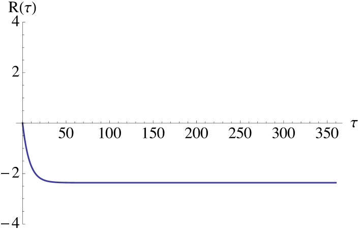
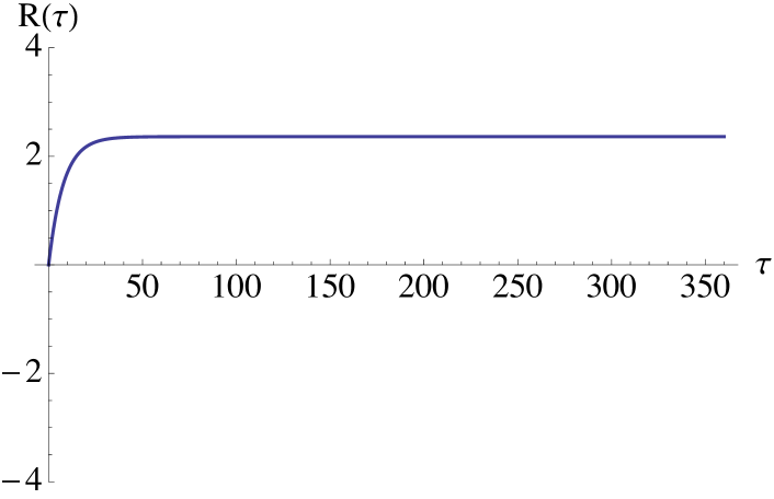
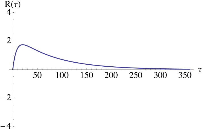
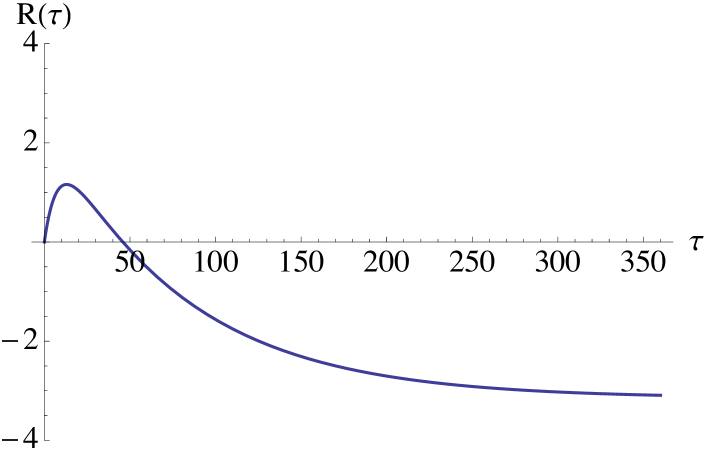
Remark 4.3.
Note that in order to get a change of sign in the risk premium one must change the level and speed of mean reversion simultaneously, see Figure 1d. It is not possible to get the sign change by using solely the Esscher transform, or only modifying the speed of mean reversion of the factors.
5. Geometric spot model
The second model for the spot price is the geometric one. We define the geometric spot price model by
| (5.1) |
where is a fixed time horizon. The process is assumed to be deterministic and it accounts for the seasonalities observed in the spot prices. The forward and the swap contracts are defined analogously to the arithmetic model.
Proposition 2.
The forward price in the geometric spot model is given by
In the particular case it holds that
Proof.
Denote by the sigma algebra generated by the process up to time Then, we have that
On the other hand, the dynamics of can be written, for as
Then, we get
Now, taking into account that has independent increments for using a stochastic version of Fubini’s Theorem and the exponential moments formula for Poisson random measures we obtain
In the last equality we have used the definition of and the change of variable Finally, combining the previous expression with the expression for with i.e., with we get the result ∎
Remark 5.1.
Note that can be infinite. In the case if then However, if then if and only if
| (5.2) |
Condition imposes some restrictions on the parameters of the model and For consider the function It is easy to see that this function is strictly positive and achieves its maximum at with value Then, it is natural to impose the following assumption on the model parameter that guarantees that condition is satisfied for all :
Assumption 2 ().
We assume that and satisfy
for some
Obviously, if then assumption is satisfied. Suppose that then if we choose close to zero the value of must be bounded away from zero, and viceversa, for assumption to be satisfied.
The risk premium in the geometric case becomes:
Theorem 5.2.
The risk premium for the forward price in the geometric spot model is given by
Proof.
This follows immediately from Proposition 2. ∎
The risk premium in the geometric case becomes hard to analyse due to the presence of the conditional expectation in the last term, involving the jump process with respect to . In the remainder of this Section we shall rather exploit the affine structure of the model to analyse the risk premium.
5.1. An analysis of the risk premium based on the affine structure
An alternative way of computing which can provide semi-explicit expressions, is to use the affine structure of Let be the Lévy exponents associated to the affine characteristics in Remark 3.2, i.e.,
We find the following:
Theorem 5.3.
Let Assume that there exist functions belonging to satisfying the generalised Riccati equation
| (5.3) |
and the integrability condition
| (5.4) |
Then,
and
| (5.5) | ||||
Proof.
The result is a consequence of Theorem 5.1 in Kallsen and Muhle-Karbe [18]: Making the change of variable , the ODE (5.3) is reduced to the one appearing in items 2. and 3. of Theorem 5.1 in Kallsen and Muhle-Karbe [18]. The integrability assumption (5.4) implies conditions 1. and 5., in Theorem 5.1, and condition 4. in that same Theorem is trivially satisfied because and are deterministic. Hence, the conclusion of Theorem 5.1 in Kallsen and Muhle-Karbe [18], with holds and we get
| (5.6) |
The result on the risk premium now follows easily. ∎
A couple of remarks are in place.
Remark 5.4.
The applicability of Theorem 5.3 is quite limited as it is stated. This is due to the fact that it is very difficult to see a priori if there exist functions belonging to satisfying equation One has to study existence and uniqueness of solutions of equation and the possibility of extending the solution to arbitrary large We study this problem in Theorem 5.7.
Remark 5.5.
Note that the previous system of autonomous ODEs can be effectively reduced to a one dimensional non autonomous ODE. We have that for any , the solution of the second equation is given by . Plugging this solution to the first equation we get the following equation to solve for
| (5.7) |
with initial condition The equation for is solved by integrating i.e.,
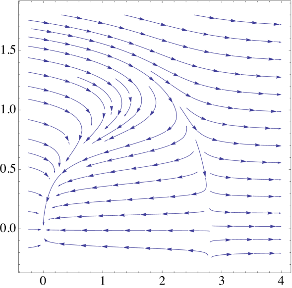
As we have already indicated, we cannot in general find the explicit solution of the system of ODEs in Theorem 5.3, and has to rely on numerical techniques. However, the main problem is to ensure the existence and uniqueness of global solutions. Before stating our main result on this question, we introduce some notation and a technical lemma.
Lemma 5.6.
Let be the function defined by
| (5.8) |
where and consider the set
Then, we have that:
-
(1)
For any there exists a unique global minimum of the function which is attained at
(5.9) with value
(5.10) -
(2)
The function is strictly decreasing in and strictly increasing in
-
(3)
For fixed, one has that when and when
-
(4)
The set coincides with the set
Moreover, for we have the following:
-
(a)
If is such that then such that
-
(b)
If is such that then there exists a unique such that
(5.11) and for all one has
-
(a)
-
(5)
For there exists a unique zero of denoted by As a function of is well defined on strictly increasing, with and
Proof.
Proof of : According to Remark 2.2 we have that
which yields that there exists a unique for and such that attains a global minimum. In fact, solves
Moreover, by Remark 2.2 again, we have that is a strictly increasing function and, hence, it has a well defined inverse which yields that and are given by equations and respectively.
Proof of It follows from the fact that and .
Proof of It follows from the monotonicity of and the explicit expression of given by equation Note that, as a function of is a strictly decreasing, continuous function in
Proof of and For any note that
and if Therefore, if then for any On the other hand, if we have that Moreover, defining the function and taking into account that and,
we can apply the implicit function theorem to the equation that ensures that there exists a neighborhood of in which we can write the root of as a function of Moreover, in we have that
which is positive as long as
This yields that is a well defined and strictly increasing function of for , where is the root of equation
Moreover, and If the existence of follows from Bolzano’s Theorem and the uniqueness from the fact that is strictly decreasing in ∎
We can now state our main result:
Theorem 5.7.
If and then are for any Moreover,
and
where or
Proof.
First, recall from Remark 5.5 that the existence and uniqueness of the system of ODEs in Theorem 5.3 can be reduced to establish existence and uniqueness for the one dimensional non autonomous equation (5.7). We have to study the time dependent vector field
Consider
and define
On the other hand, for one has that
and
Moreover, note that
Hence, the vector field is well defined (i.e., finite) and locally Lipschitz in Then, by the Picard-Lindelöf Theorem (see Theorem 3.1, page 18, in Hale [16]) we have local existence and uniqueness for with
Let us consider the autonomous vector field
Then, as for using a comparison theorem we have that the solution for the ODE associated to and starting at is bounded above by the corresponding solution to the ODE associated to which we will denote by By Lemma 5.6, if there exists a unique such that for and This yields that the solution is defined for and monotonously converges to which is a stationary point of Hence, the solution is bounded by and defined for To prove that actually converges to zero it is convenient to look at the dimensional system
| (5.12) |
with the corresponding vector fields
Note that is a stationary point, that for , that for and for Hence, the region is invariant for this vector field, i.e., a solution that enters cannot leave Moreover, we have that the vector field evaluated at the line has the form
i.e., By Lemma 5.6, it then follows that for In addition, if we have that This means that for which can be extended to for some Note that is in the domain of attraction of the stationary point As and , we have that for and, hence, it converges to when tends to infinity. Note that we can look at the system as a perturbed linear system, i.e.,
where
and
Hence, that converges to zero exponentially fast follows from Theorem 3.1.(i), Chapter VII, in Hartman [17]. On the other hand, by Remark 5.5 and the monotone convergence theorem, we have that
To prove that the previous integral is finite, note first that, as and the function is increasing we have that But, by definition
which yields that
which is bounded. Hence, it suffices to prove that converges to zero faster than for some when tends to infinity. We have that
because converges to zero exponentially fast and by bounded convergence. ∎
An immediate consequence of the Theorem above is that the forward price will be equal to the seasonal function in the long end, that is, when and , it holds that
Note that to have this limiting de-seasonalized forward price, we must compute an integral of a nonlinear function of , for which we do not have any explicit solution available. Note that from part 4(b) in Lemma 5.6 we have if and , for a uniquely defined . We recall that is the speed of mean reversion of the stochastic volatility , and is the maximal exponential integrability of , the subordinator driving the same process. Thus, we must choose less that , by a distance given by the inverse of the speed of mean reversion. Then we know there exists an interval of ’s for which we can reduce the speed of mean reversion of . Here we see clearly the competition between the jumps of and the speed of mean reversion of .
We note that if we just change the levels of mean reversion, that is assuming then we can compute the risk premium more explicitly. This case will correspond to an Esscher transform of both the Brownian motion driving and the subordinator driving .
Proposition 3.
Suppose that and Then the forward price is given by
and the risk premium by
| (5.13) | ||||
Proof.
Note that the system of generalised Riccati equations to solve is
With respect to and this coincides with the one satisfied by and Hence, and we just need to integrate the equation for to obtain that
to conclude. ∎
Next, we present two examples where we apply the previous results.
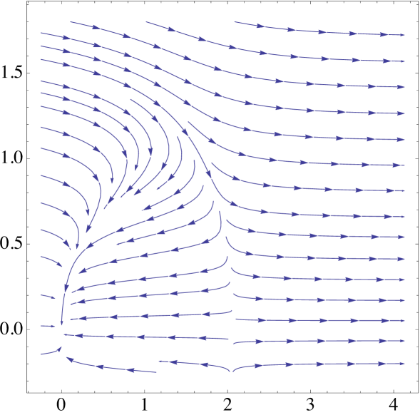
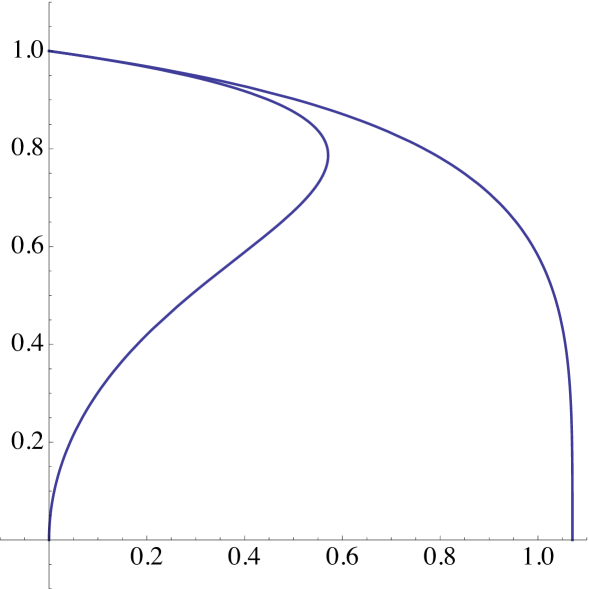
Example 5.8.
We start by the simplest possible case. Assume that the Lévy measure is that is, the Lévy process has only jumps of size In this case and, hence, We have that and Therefore, the associated generalised Riccati equation is given
| (5.14) |
In this example
which does not depend on By Lemma 5.6, attains its minimum at
and equation (5.11) reads
| (5.15) |
Using the Lambert W function, i.e., the function defined by W we get that the root of equation (5.15) is given by
Hence, according to Lemma 5.6, the set and if there exists a unique root of equation satisfying . This root is given by
See Figure 2 for a graphical illustration of this case.
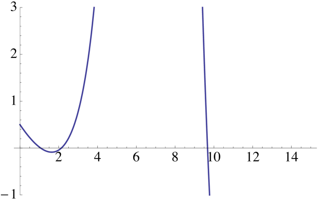
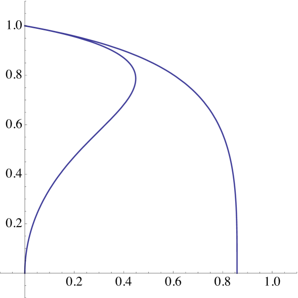
Example 5.9.
Assume that the Lévy measure is that is, is a compound Poisson process with intensity and exponentially distributed jumps with mean In this case and, hence, We have that and Therefore, the associated generalised Riccati equation is given by
| (5.16) |
In this example,
By Lemma 5.6, attains its minimum at
and equation (5.11) reads
| (5.17) |
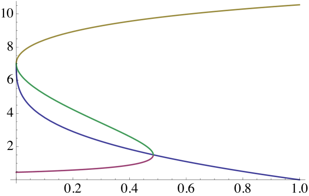
According to Lemma 5.6, if then such that If then there exists such that for all and is the unique solution of equation lying in Making the change of variable equation is reduced to a cubic equation and we get
where
Finally, if there exists a unique root of equation satisfying . Making the change of variable we can reduce the equation to the cubic equation
which can be solved explicitely. Inverting the change of variable, we can get an explicit expression for We refrain to write this explicit formula because it is too lengthy.
See Figure 3 for some graphical illustrations of this example.
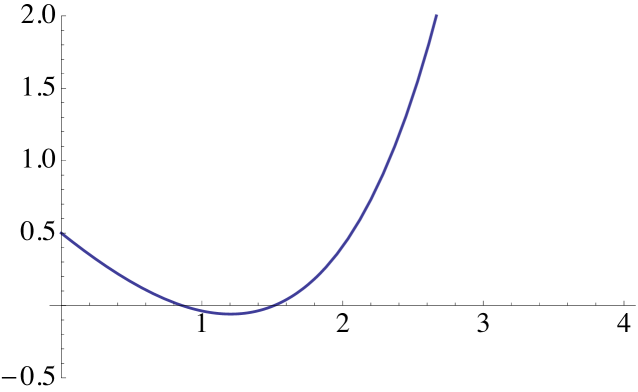
5.2. Discussion on the risk premium
The next step is to analyse qualitatively the possible risk premium profiles that can be obtained using our change of measure. In particular, we are interested to be able to generate risk profiles with positive values in the short end of the forward curve and negative values in the long end. In what follows we shall make use of the Musiela parametrization and we will slightly abuse the notation by denoting by We also fix the parameters of the model under the historical measure i.e., and and study the possible sign of in terms of the change of measure parameters, i.e., and and the time to maturity
In contrast to the arithmetic model, the present time enters into the risk premium not only through the stochastic components but also through the stochastic volatility Moreover, in the geometric model, the risk premium will also depend on the parameters and which change the level and speed of mean reversion for the volatility process. We are going to study the cases and the general case separately. Moreover, in order to graphically illustrate the discussion we plot the risk premium profiles obtained assuming that the subordinator is a compound Poisson process with jump intensity and exponential jump sizes with mean That is, will have the Lévy measure given in Example 3.1. We shall measure the time to maturity in days and plot for different maturity periods. We fix the parameters of the model under the historical measure using the same values as in the arithmetic case, i.e.,
Finally, in the sequel, we are going to suppose that we are under the assumptions of Theorem 5.7, i.e., the values are such that and and are globally defined and the exponential affine formula holds.
The following lemma will help us in the discussion to follow.
Lemma 5.10.
The sign of the risk premium is the same as the sign of the function
Moreover,
| (5.18) | ||||
and
| (5.19) |
Proof.
That the sign of is the same as the sign of is obvious from equation (5.5) in Theorem 5.3. From the expression for in Proposition 2, we can deduce that
Furthermore, by Theorem 5.7, one has that
which yields equation (5.18). On the other hand, as and when tends to zero, we have
which yields equation (5.19). The proof is complete. ∎
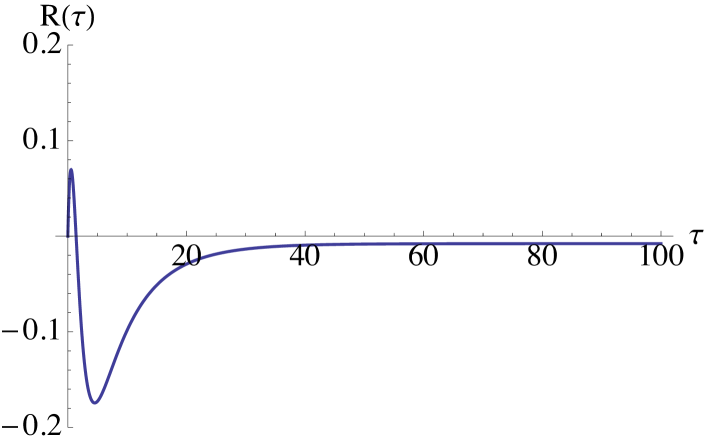
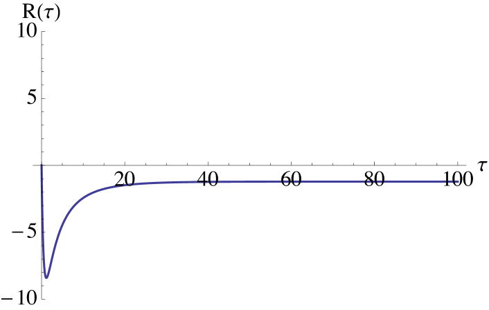
We now continue with investigating in more detail the different cases of our measure change.
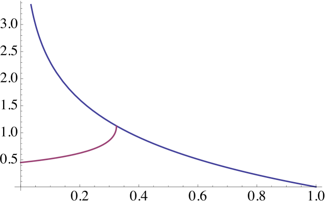
-
•
Changing the level of mean reversion (Esscher transform): Setting the probability measure only changes the levels of mean reversion for the factor and the volatility process Although the risk premium is stochastic, its sign is deterministic. According to Proposition 3, we have that the sign of is equal to the sign of
Moreover, by Lemma 5.10, equations (5.18)-(5.19), and the fact that we get
and
Note that we can write
and that for is strictly positive. Hence, if we choose small enough and large enough , we obtain a risk premium which is positive in the short end of the forward curve, and negative in the long end. Note that must be chosen negative. Figure 4 shows graphically two possible risk premium curves for given parameters as an illustration. We recall from Benth and Ortiz-Latorre [9] that for a two-factor mean reverting stochastic dynamics of the spot price without stochastic volatility, we obtain similar deterministic risk premium profiles.

(a) 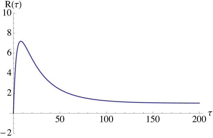
(b) Figure 5. Risk premium profiles when is a Compound Poisson process with exponentially distributed jumps. We take Case -
•
Changing the speed of mean reversion: Setting the probability measure only changes the levels of mean reversion for the factor and the volatility process Both the risk premium and its sign are stochastic. According to Lemma 5.10, we have that the sign of is equal to the sign of
Moreover,
and
Note that
and using a comparison theorem for ODEs, Theorem 6.1, page 31, in Hale [16], we get that Hence, the risk premium will approach to a non negative value in the long end of the forward curve. In the short end, it can be positive or negative and stochastically varying with In Figure 5 we show two different risk premium curves, where we in particular notice the different convexity behaviour in the short end. As all the risk premia curves will be positive in the long end, it is not very realistic from the practical point of view to have
(a) 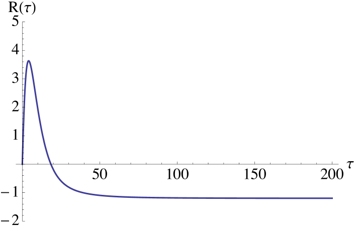
(b) Figure 6. Risk premium profiles when is a Compound Poisson process with exponentially distributed jumps. We take -
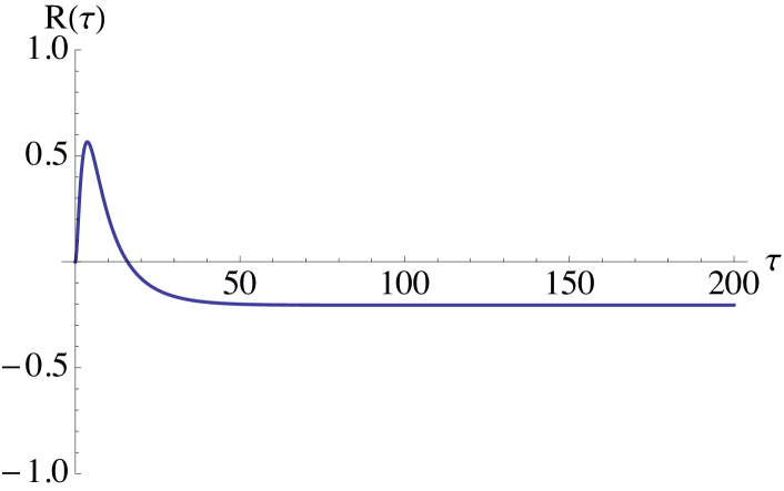
•
Changing the level and speed of mean reversion simultaneously: In the general case we modify the speed and level of mean reversion for the factor and the volatility process simultaneously. According to Lemma 5.10, we have that
and
If we choose then we need to prove that for some and we have
(5.20) in order to ensure a risk premium that changes sign from positive to negative. In fact, inequality 5.20 holds by choosing small enough and a large negative number, because . See Figure 6 for two cases.
Remark 5.11.
In contrast to the arithmetic case, one can get a positive risk premium for short time to maturity that rapidly changes to negative by just changing the parameters of the Esscher transform, see Figure 4. Similarly to the arithmetic case, it is not possible to get the sign change by just modifying the speed of mean reversion of the factors, see Figure 5.
References
- [1] Barndorff-Nielsen, O. E., and Shephard, N. (2001). Non-Gaussian Ornstein-Uhlenbeck models and some of their uses in economics. J. Roy. Stat. Soc. B, 63(2), pp. 167–241 (with discussion).
- [2] Benth, F. E. (2011). The stochastic volatility model of Barndorff-Nielsen and Shepard in commodity markets. Math. Finance, 21, pp. 595–625.
- [3] Benth, F. E., and Šaltytė Benth, J. (2011). Weather derivatives and stochastic modelling of temperature. Intern. J. Stoch. Analysis, Vol 2011, Article ID 576791, 21 pages (electronic).
- [4] Benth, F. E., and Šaltytė Benth, J. (2013). Modeling and Pricing in Financial Markets for Weather Derivatives. World Scientific, Singapore.
- [5] Benth, F. E., Šaltytė Benth, J. and Koekebakker, S. (2008). Stochastic Modelling of Electricity and Related Markets. World Scientific, Singapore.
- [6] Benth, F. E., Cartea, A., and Kiesel, R. (2008). Pricing forward contracts in power markets by the certainty equivalence principle: explaining the sign of the market risk premium. J. Banking Finance, 32(10), pp. 2006–2021.
- [7] Benth, F. E., Cartea, A., and Pedraz, C. (2013). In preparation.
- [8] Benth, F. E., Koekebakker, S., and Taib, I. B. C. M. (2013). Stochastic dynamical modelling of spot freight rates. To appear in IMA J. Manag. Math.
- [9] Benth, F. E. and Ortiz-Latorre, S. (2013). A pricing measure to explain the risk premium in power markets. arXiv:1308.3378 [q-fin.PR]
- [10] Dornier, F., and Querel, M. (2000). Caution to the wind. Energy & Power Risk Manag., weather risk special report. August issue, pp. 30–32.
- [11] Eydeland, A., and Wolyniec, K. (2003). Energy and Power Risk Management, John Wiley & Sons, Hoboken, New Jersey.
- [12] Garcia, I., Klüppelberg, C., Müller, G. (2011). Estimation of stable CARMA models with an application to electricity spot prices. Statist. Modelling, 11(5), pp. 447–470.
- [13] Geman, H. (2005). Commodities and Commodity Derivatives, John Wiley & Sons, Chichester.
- [14] Geman, H., and Vasicek, O. (2001). Forwards and futures on non-storable commodities: the case of electricity. RISK, August.
- [15] Gerber, H. U., and Shiu, E. S. W. (1994). Option pricing by Esscher transforms. Trans. Soc. Actuaries, 46, pp. 99–191 (with discussion).
- [16] Hale, J. (1969). Ordinary Differential Equations, Pure and Applied Mathematics, Vol. XXI. Wiley-Interscience, New York.
- [17] Hartman, P. (1964). Ordinary Differential Equations, John Wiley & Sons, Inc, New York.
- [18] Kallsen, J. and Muhle-Karbe J. (2010). Exponentially affine martingales, affine measure changes and exponential moments of affine processes. Stoch. Proc. Applic. , 120, pp. 163–181.
- [19] Kolos, S. P., and Ronn, E. I. (2008). Estimating the commodity market price of risk for energy prices. Energy Econ., 30, pp. 621–641.
- [20] Lucia, J., and Schwartz E. (2002). Electricity prices and power derivatives: evidence from the Nordic Power Exchange. Rev. Deriv. Research, 5(1), pp. 5–50.
- [21] Protter, P. E. (2004). Stochastic Integration and Differential Equations, 2nd Edition. Springer Verlag, Berlin Heidelberg New York.
- [22] Shiryaev, A. N. (1999). Essentials of Stochastic Finance, World Scientific, Singapore.
- [23] Schwartz, E. S. (1997). The stochastic behaviour of commodity prices: Implications for valuation and hedging. J. Finance, LII(3), pp. 923–973.
- [24] Schwartz, E. S., and Smith, J. E. (2000). Short-term variations and long-term dynamics in commodity prices. Manag. Sci., 46(7), pp. 893–911.
- [25] Trolle, A. B., and Schwartz, E. S. (2009). Unspanned stochastic volatility and the pricing of commodity derivatives. Rev. Financial Studies, 22(11), pp. 4423–4461.