A CMOS Tailed Tent Map for the Generation of Uniformly Distributed Chaotic Sequences
Abstract
This paper describes the design of a modified tent map characterized by a uniform probability density function. The use of this map is proposed as an alternative to the tent map and the Bernoulli shift. It is shown that practical circuits implementing the latter two maps may possess parasitic stable equilibria, fact which would prevent the desired chaotic behavior of the system. On the other hand, commonly used strategies to avoid the parasitic equilibria onset also affect the uniformity of the probability density function. Conversely, the use of the proposed tailed tent map allows to assure a certain degree of parameter deviation robustness, without compromising on the statistical properties of the system.
I Introduction
Discrete time chaotic systems based on simple, one-dimensional, piecewise linear maps can be conveniently implemented using current mode operation [1]. Low circuit complexity makes them appealing for many applications, like secure communication schemes [2], noise generators and analog random number generation for stochastic neural models [3]. Design requirements can be posed either on the spectrum or on the probability distribution of the chaotic signal. For instance, the random number generator needed in [3] should produce samples characterized by a uniform probability density function (PDF).
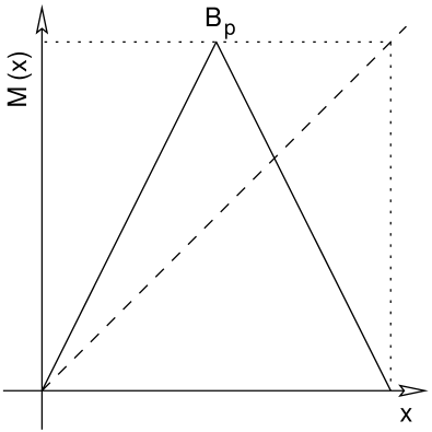
Although systems based on the tent map (Fig. 1A) and on the Bernoulli shift satisfy this requirement, their implementation [1, 4] is not completely straightforward, due to the possible onset of parasitic stable equilibrium points, as result of the unavoidable errors introduced by the physical realization of the electronic devices. Since this fact would not allow the desired chaotic behavior, special strategies must be adopted to make the system robust to parameter deviation. Unfortunately, commonly adopted solutions [4] also prevent the achievement of a uniform PDF.
(A)
(B)
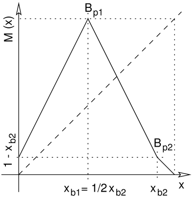
The aim of this paper is to show that a one-dimensional system based on a modified version of the tent map, referred as tailed tent map (Fig. 1B), possesses both a uniform PDF and a chaotic behavior inherently robust to implementation errors, being better suited for carrying out, for instance, the random number generator needed in [3]. In order to show the feasibility of the system, a design in a standard , n-well, single-poly CMOS technology is also proposed. Several circuit simulations confirm the uniform distribution of the samples produced by the system.
I-A Mathematical background
Let be an interval of the real line and consider the one-dimensional dynamical system
| (1) |
where is a nonsingular transformation of into itself. When designing a pseudo random number or a noise generator based on system (1) two properties are particularly important, namely i) chaotic behavior and ii) uniform probability density.
-
i)
Chaotic behavior is assured when the system (1) has a positive Lyapunov exponent, defined as [5]:
(2) Roughly speaking, the Lyapunov exponent is an index of the sensitivity of the system to initial conditions and therefore of its level of unpredictability. From (2) it immediately follows that systems based on everywhere expanding maps (for which ) are chaotic.
-
ii)
Consider an interval and let be the relative characteristic function. Then, the “average time” spent in by an orbit originating in may be defined as
(3) where is the -th iterate of the map. Note that if limit (3) exists, it depends on the choice of the initial condition . Birkhoff ergodic theorem [6] gives a sufficient condition for the existence of limit (3) “almost” independently from . In particular, it states that, if is measure preserving111 is said to be measure preserving if a measure exists such that for any measurable set . and ergodic then there is a unique PDF for such that
(4) for any measurable . Basically, ergodicity provides that any initial condition randomly chosen in leads to a trajectory characterized by the same statistical properties. Furthermore, ergodicity enables extraction of information about time-based statistics from the a priori knowledge of the PDF. In particular, it can be shown that, if is ergodic, the PDF is the unique invariant under the Perron-Frobenius operator [6] defined as
(5) namely .
In the following, we will consider the design of the tailed tent map in order to obtain an ergodic system and we will thus determine its uniform PDF as a fixed point of . Eventually, we will verify its robustness to breakpoints misplacement both via analytic considerations and by approximating using time series data extracted from simulations.
II Systems based on the tent map
Consider a tent map based system (1), namely assume and
| (6) |
Since the map is everywhere expanding, the system is chaotic. Moreover, it can be proved that the system is ergodic and characterized by a uniform PDF [5].

Transistors , and Inv act as an active rectifier: when is positive (negative) () is on and () is off. Since current mirrors and have a 2:1 ratio, one obtains . The simulated static characteristic is represented in Fig. 3A and is the same as (6) apart from an uninfluential change of the reference system. Considering the implementation of equation (1) by a current mode circuit, the necessary delay operation can be realized by cascade connecting two switched current (SI) sample and hold stages with complementary phase clock [1].
II-A Parasitic stable equilibrium and strategies to avoid it
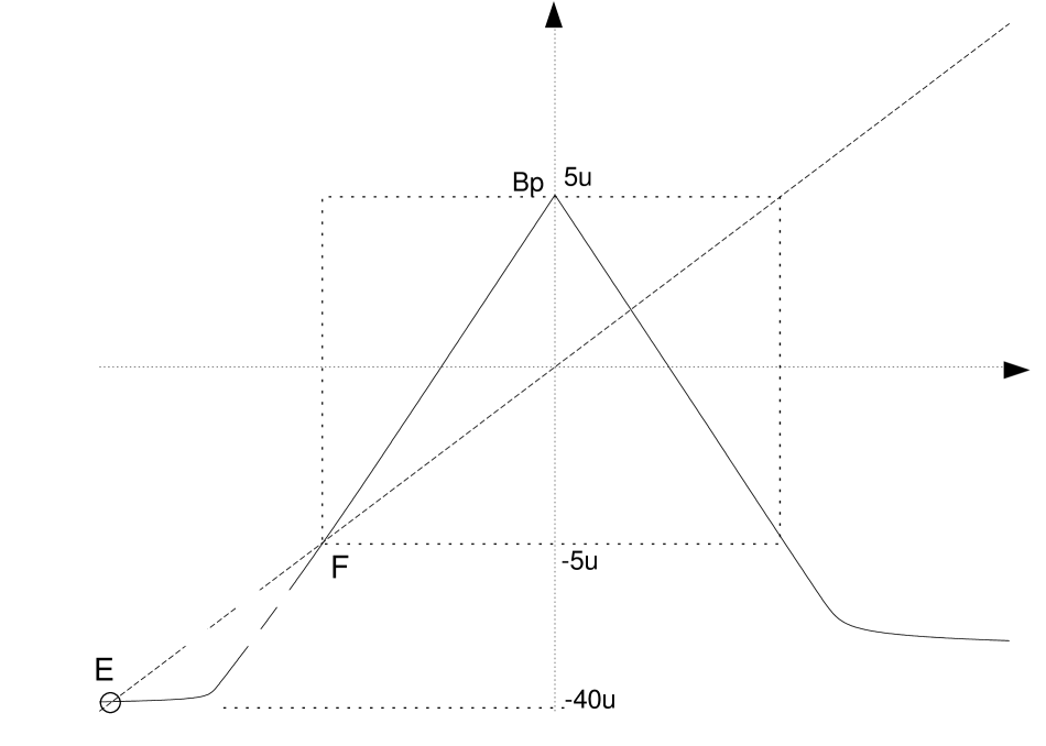
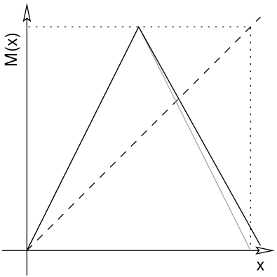
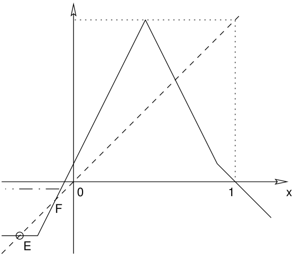
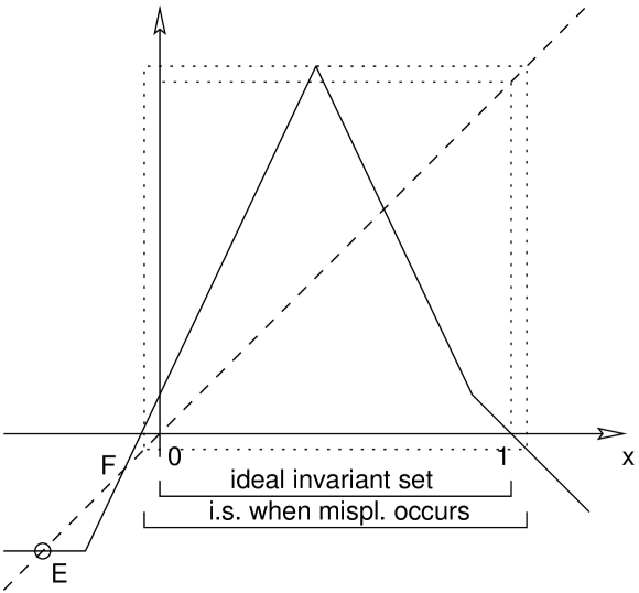
When the map is implemented using an analog circuit, some misplacement of the breakpoint is unavoidable. If the ordinate of the breakpoint exceeds its assigned value due to a slope error, a parasitic stable equilibrium is introduced. In order to see how this happens, it is necessary to consider the circuit static characteristic outside the map domain. Due to the fact that the current mirrors or the current rectifier transistors (Fig. 2) reach their maximum allowable current, the map slope decreases and flattens, as shown in Fig. 3A. As a consequence a parasitic equilibrium point exists (point E in Fig. 3) characterized by , i.e. the equilibrium is stable. Although this equilibrium always exists, it ideally lies out of the map invariant set. On the contrary, if the breakpoint ordinate is greater than its assigned value (independently of the magnitude of the misplacement), the map invariant set abruptly expands, including also point . Therefore, after a transient phase, the system trajectory will converge towards it, as schematically represented in Fig. 3B. The abrupt expansion of the invariant set is due to the fact that its closure contains the unstable equilibrium point . As soon as the invariant set grows to include in its interior it must also contain the whole interval .
(A)

(B)
Note that besides breakpoint misplacement, also noise added to the system state may allow the system trajectory to converge to E.
In order to avoid this problem, several strategies can be used. All of them are based on small modifications of the map222 Without loss of generality we will refer our considerations to normalized maps defined in . and are equivalent to designing a system whose breakpoint ordinate is less than 1, to assure an adequate margin. Two typical solutions are shown in Fig. 4.
(A)
(B)
The margin one must allow mainly depends on three factors:
-
1.
the maximum random error one can expect for the circuit static characteristic. This originates mainly from transistors mismatching;
-
2.
the error introduced by the two SI sample and hold performing the delay operation. This is mainly due to clock feedthrough and appears as an undesired signal added to the system state;
-
3.
the error due to the dynamic response of the current comparator used to implement the breakpoint (Fig. 2). This error manifests itself as a sort of hysteresis and appears when the circuit has to switch immediately over or below threshold.
In particular, if speed is an important requirement, transistors dimensions must be reduced in order to contain parasitic capacitances effects and the first factor will have great importance. On the other hand, if a low-power circuit is desired, one has to accept a worsening of the current comparator dynamic response and a consequent increased relevance of the third factor. Therefore, particularly in fast, low power systems the required margin can be appreciable.
II-B Pitfalls in the strategies to prevent convergence to parasitic equilibria
Adopting one of the above mentioned strategies implies sacrificing PDF uniformity. For instance, Fig. 5 shows the consequences on the PDF of modifying the map as shown in Fig. 4A.

(A)

(B)
The graphs are obtained simulating system (1) for a tent map in which the ordinate of has been decreased by 2%, i.e. for a system tolerant to breakpoint misplacements up to 2%. In Fig. 5A it is represented the case in which no misplacement occurs (ideal case), while Fig. 5B shows the worst case in which a 2% misplacement takes the breakpoint even further down.
By similar considerations, it can be seen that systems based on the Bernoulli shift suffer from the same inconveniences mentioned above [4].
III The new approach: systems based on the tailed tent map
The tailed tent map (Fig. 1B) is a parametric map, whose secondary breakpoint also defines the position of the main one, namely
| (7) |
with . In the following, it will be shown that system (1) with and given by (7) has the same basic properties as the one based on the tent map, yet is more robust to implementation errors, whenever a uniform PDF is the desired goal.
III-A Basic properties
A piecewise linear map is also a Markov map if it takes partition points into partition points, namely a partition , , , exists such that if then . It is easy to show that whenever is a rational number, (7) is a Markov map. Moreover, in this case, satisfies also the conditions of Definition 3 in [7] which assure the PDF unicity and the ergodicity of the map. Thus, it is easy to prove that
| (8) |
is the invariant PDF. In fact, it can be easily seen that as any has a finite number of counterimages, then can be also written as
| (9) |
Thus, by substituting (8) in (9) one immediately gets
Knowing the invariant PDF, the Lyapunov exponent for the map can be computed as [5]
| (10) |
which leads to , proving system chaoticity.
III-B Inherent robustness of the map
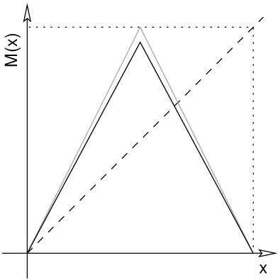
First of all, note that one can design the map in such a way that point E does not exist, as shown in Fig. 6A (dot-dashed line). Furthermore, even if E exists, the alteration in the invariant set consequent to breakpoint misplacement is now graceful, i.e. the smaller the misplacement the smaller the invariant set change, as long as this set does not include the unstable equilibrium point . Therefore, up to a certain misplacement the invariant set can grow without including E (Fig. 6B). More precisely, the lower , the higher the system tolerance.
(A)
(B)
As a consequence, a system based on the tailed tent map can be designed without having to compromise on the PDF in principle.
The effect of implementation errors is shown in Fig. 7.

(A)

(B)
In particular, Fig. 7A is the ideal case (i.e. the map is implemented correctly) and Fig. 7B represents the case of a 2% misplacement. The superiority of the case in Fig. 7A over the one in Fig. 5A is evident and also the case in Fig. 7B is more similar to an ideal uniform PDF than the one in Fig. 5B, since the latter even presents a much larger range of values characterized by null probability density. The performance improvement becomes even more visible when one considers probability distributions rather than densities.
III-C Circuit CMOS implementation and performances
Fig. 8 shows a schematic of the proposed circuit implementation for the tailed tent map. Its left side is the same as in Fig. 2, while it right side allows to obtain the slope variation necessary to carry out the “tail.” Assuming that current mirrors and have a ratio, the output current is , where , namely a tailed tent map apart from the usual change of system reference.
Note that the extra silicon area requested to generate the tailed tent map is only a small part of the area used for the complete circuit. In fact, this includes two sample and hold circuits which use a large proportion of the total area.

Fig. 9 shows the results of device level simulations for the circuit in Fig. 8 designed using a standard CMOS technology. To obtain high linearity for the map branches, high swing cascode mirrors have been used while, to improve maximum frequency operation, a careful design of the sample and hold stage has also been considered. Fig. 9A shows a typical chaotic waveform for . Fig. 9B represents the approximation of the PDF obtained by a post-processing executed on the transient analysis output, for a 750 KHz operating frequency. Deviation from the ideal line is not only due to circuit misbehavior, but also to the finite number of samples used to extract the PDF.
In conclusion, the new proposed solution shows several improvements compared to previously published results, with respect to the achievable PDF [1] and parameter deviation robustness [4].

(A)

(B)
Acknowledgments
Sergio Callegari would like to thank Prof. P. U. Calzolari, Prof. G. Masetti and the EU Erasmus Project for allowing his research period at King’s College, London.
References
- [1] J. T. Bean and P. J. Langlois. A current mode analog circuit for tent maps using piecewise linear functions. In Proceedings of IEEE ISCAS, volume 6, pages 125–128, London, may 1994.
- [2] M. Hasler. Syncronization principles and applications. In Proceedings of the IEEE ISCAS (Tutorials), pages 314–327, London, may 1994.
- [3] T. G. Clarkson, C. K. Ng, and J. Bean. Review of hardware pRAMs. Neural Networks World, (5):551–564, 1993.
- [4] M. Delgado-Restitudo, F. Medeiro, and A. Rodríguez-Vázquez. Nonlinear, switched current cmos ic for random signal generation. Electronic Letters, (25):2190–2191, 1993.
- [5] E. Ott. Chaos in dynamical systems. Cambridge University Press, 1993.
- [6] A. Lasota and M. C. Mackey. Chaos, Fractals and Noise. Stochastic Aspects of Dynamics. Springer-Verlag, 2nd edition, 1995.
- [7] A. Boyarsky and M. Scarowsky. On a class of transformations which have unique absolutely continuous invariant measures. Transactions of the American Mathematical Society, 255:243–262, Nov 1979.