22email: njm11@mails.tsinghua.edu.cn 33institutetext: Zhenbo Wang ( 🖂 )44institutetext: Department of Mathematical Sciences, Tsinghua University, Beijing, 100084, China
44email: zwang@math.tsinghua.edu.cn 55institutetext: Fabrice Talla Nobibon 66institutetext: Postdoctoral researcher for Research Foundation–Flanders
ORSTAT, Faculty of Economics and Business, KU Leuven, Belgium
66email: Fabrice.TallaNobibon@kuleuven.be 77institutetext: Roel Leus 88institutetext: ORSTAT, Faculty of Economics and Business, KU Leuven, Belgium
88email: Roel.Leus@kuleuven.be
A Combination of Flow Shop Scheduling and the Shortest Path Problem††thanks: A preliminary version of this paper has appeared in the Proceedings of 19th Annual International Computing and Combinatorics Conference (COCOON’13), LNCS, vol. 7936, pp. 680–687.
Abstract
This paper studies a combinatorial optimization problem which is obtained by combining the flow shop scheduling problem and the shortest path problem. The objective of the obtained problem is to select a subset of jobs that constitutes a feasible solution to the shortest path problem, and to execute the selected jobs on the flow shop machines to minimize the makespan. We argue that this problem is NP-hard even if the number of machines is two, and is NP-hard in the strong sense for the general case. We propose an intuitive approximation algorithm for the case where the number of machines is an input, and an improved approximation algorithm for fixed number of machines.
Keywords:
approximation algorithm; combination of optimization problems; flow shop scheduling; shortest path1 Introduction
Combinatorial optimization is an active field in operations research and theoretical computer science. Historically, independent lines separately developed, such as machine scheduling, bin packing, travelling salesman problem, network flows, etc. With the rapid development of science and technology, manufacturing, service and management are often integrated, and decision-makers have to deal with systems involving several characteristics from more than one well-known combinatorial optimization problem. To the best of our knowledge, the combination of optimization problems has received only little attention in literature.
Bodlaender et al. (1994) studied parallel machine scheduling with incompatible jobs, in which two incompatible jobs cannot be processed by the same machine, and the objective is to minimize the makespan. This problem can be considered as a combination of parallel machine scheduling and the coloring problem. Wang and Cui (2012) studied a combination of parallel machine scheduling and the vertex cover problem. The goal is to select a subset of jobs that forms a vertex cover of a given graph and to execute these jobs on identical parallel machines to minimize the makespan. They proposed an -approximation algorithm for this problem. Wang et al. (2013) have investigated a generalization of the above problem that combines the uniformly related parallel machine scheduling problem and a generalized covering problem. They proposed several approximation algorithms and mentioned as future research other combinations of well-known combinatorial optimization problems. This is the core motivation for this work.
Let us consider the following scenario. We aim at building a railway between two specific cities. The railway needs to cross several adjacent cities, which is determined by a map (a graph). The processing time of manufacturing the rail track for each pair of cites varies between the pairs. Manufacturing a rail track between two cities in the graph is associated with a job. The decision-maker needs to make two main decisions: (1) choosing a path to connect the two cities, and (2) deciding the schedule of manufacturing the rail tracks on this path in the factory. In addition, the manufacturing of rail tracks follows several working stages, each stage must start after the completion of the preceding stages, and we assume that there is only one machine for each stage. We wish to accomplish the manufacturing as early as possible, i.e. minimize the last completion time; this is a standard flow shop scheduling problem. How should a decision-maker choose a feasible path such that the corresponding jobs can be manufactured as early as possible? This problem combines the structure of flow shop scheduling and the shortest path problem. Following the framework introduced by Wang et al. (2013), we can regard our problem as a combination of those two problems.
Finding a simple path between two vertices in a directed graph is a basic problem that can be polynomially solved (Ahuja et al., 1993). Furthermore, if we want to find a path under a certain objective, various optimization problems come within our range of vision. The most famous one is the classic shortest path problem, which can be solved in polynomial time if the graph contains no negative cycle, and otherwise it is NP-hard (Ahuja et al., 1993). Moreover, many optimization problems have a similar structure. For instance, the min-max shortest path problem (Kouvelis and Yu, 1997) studies a problem with multiple weights associated with each arc, and the objective is to find a directed path between two specific vertices such that the value of the maximum among all its total weights is minimized. The multi-objective shortest path problem (Warburton, 1987) also has multiple weights, but the objective is to find a Pareto optimal path between two specific vertices to satisfy some specific objective function.
Flow shop scheduling is one of the three basic models of multi-stage scheduling (the others are open shop scheduling and job shop scheduling). Flow shop scheduling with the objective of minimizing the makespan is usually denoted by , where is the number of machines. In one of the earliest papers on scheduling problems, Johnson (1954) showed that can be solved in time, where is the number of jobs. On the other hand, Garey et al. (1976) proved that is strongly NP-hard for .
The contributions of this paper include: (1) a formal description of the considered problem, (2) the argument that the considered problem is NP-hard even if , and NP-hard in the strong sense if , and (3) several approximation algorithms.
The rest of the paper is organized as follows. In Section 2, we first give a formal definition of the problem stated above, then we briefly review flow shop scheduling and some shortest path problems, and introduce some related algorithms that will be used in the subsequent sections. In Section 3, we study the computational complexity of the combined problem. Section 4 provides several approximation algorithms for this problem. Some concluding remarks are provided in Section 5.
2 Preliminaries
2.1 Problem Description
We first give a formal definition of our problem, which is a combination of the flow shop scheduling problem and the shortest path problem.
Definition 1
Given a directed graph with two distinguished vertices and flow shop machines, each arc corresponds with a job with processing times , , , respectively. The problem is to find a directed path , and to schedule the jobs of on the flow shop machines to yield the minimum makespan over all , where denotes the set of jobs corresponding to the arcs in .
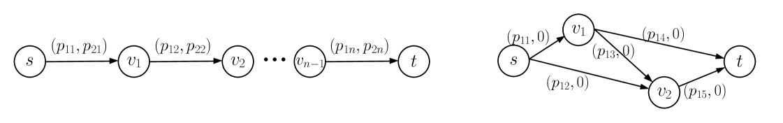
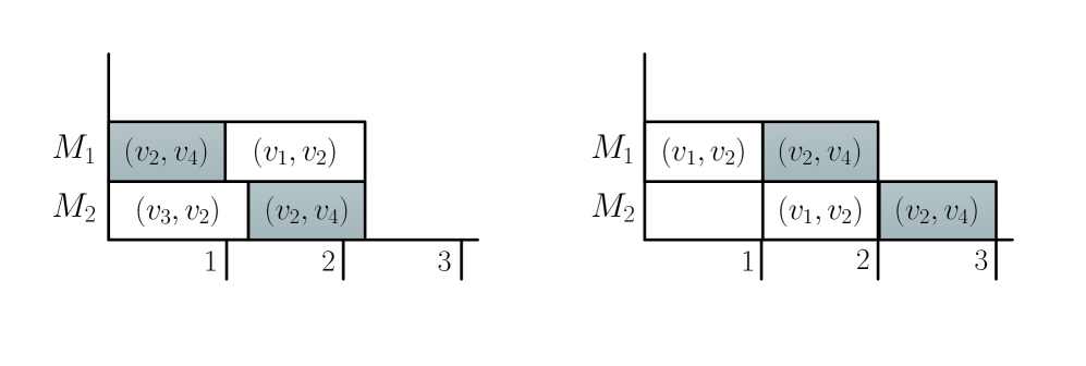
The considered problem is a combination of flow shop scheduling and the classic shortest path problem, mainly because the two optimization problems are special cases of this problem. For example, consider the following instances with . If there is a unique path from to in , as shown in the left of Fig. 1, our problem is the two-machine flow shop scheduling problem. If all the processing times on the second machine are zero, as shown in the right of Fig. 1, then our problem is equivalent to the classic shortest path with respect to the processing times on the first machine. These examples illustrate that these two optimization problems are inherent in the considered problem.
In this paper, we will use the results of some optimization problems that have a similar structure with the classic shortest path problem. We introduce the following generalized shortest path problem.
Definition 2
Given a directed graph and two distinguished vertices with . Each arc is associated with weights , and we define the vector for . The goal of our shortest path problem is to find a directed path that minimizes , in which is a given objective function and contains the decision variables such that if and only if .
For ease of exposition, we use instead of when there is no danger of confusion. Notice that is a generalization of various shortest path problems. For instance, if we consider and , where is the dot product, this problem is the classic shortest path problem. If and , where is a given number, this problem is the shortest weight-constrained path problem (Garey and Johnson, 1979). If , the problem is the min-max shortest path problem (Kouvelis and Yu, 1997). In the following sections, we will analyze our combined problem by setting appropriate weights and objective function in .
2.2 Algorithms for Flow Shop Scheduling Problems
First, we introduce some trivial bounds for flow shop scheduling. Denote by the makespan of an arbitrary flow shop schedule with job set . A feasible shop schedule is called dense when any machine is idle if and only if there is no job that can be processed at that time on that machine. For arbitrary dense flow shop schedule, we have
| (1) |
and
| (2) |
For each job, we have
| (3) |
In flow shop scheduling problems, a schedule is called a permutation schedule if all jobs are processed in the same order on each machine. Conway et al. (1971) proved that there always exists a permutation schedule which is optimal for and . In a permutation schedule, the critical job and critical path are important concepts for the analysis of related algorithms.
Suppose we are given a job set with jobs. Let be a permutation of for a three-machine (or two-machine) flow shop, and let be the corresponding schedule. For simplicity of notation, we denote the permutation and the schedule by and respectively. A directed graph is defined as follows. We define a vertex with an associated weight for each job and each machine , for (or ) and . We include arcs leading from each vertex towards , and from towards for . The total weight of a maximum weight path from to (or ), which is called a critical path, is equal to the makespan of the corresponding permutation schedule. For the three-machine case, the critical jobs with respect to are defined as the jobs and such that , , and appear in the critical path, i.e. the jobs and satisfy
| (4) |
For the two-machine case, the critical job with respect to is defined as the job such that and appear in the critical path, i.e. the job satisfies
| (5) |
Johnson (1954) proposed a sequencing rule for , which is one of the oldest results of the scheduling literature, and is commonly referred to Johnson’s rule.
In Johnson’s rule, jobs are scheduled as early as possible. This rule produces a permutation schedule, and Johnson showed that this schedule is optimal. Notice that this schedule is obtained in time.
For the general problem , Gonzalez and Sahni (1978) first presented an -approximation algorithm that runs in time by solving two-machine flow shop scheduling problems. Röck and Schmidt (1982) proposed an alternative approach by reducing the original problem to an artificial two-machine flow shop problem; this approach is called machine aggregation heuristic. They obtained a permutation by solving the artificial problem in time, and proved that it has the same performance guarantee of . Based on the machine aggregation heuristic, Chen et al. (1996) proposed an algorithm for with an improved performance guarantee of . In the same paper, they also modified the Gonzalez and Sahni’s algorithm if is odd, by partitioning the machines into two-machine flow shop scheduling problems, and one three-machine flow shop scheduling problem which was solved by their -approximation algorithm. The modified algorithm has the same performance ratio if is even, and an improved ratio if is odd. It is known that a PTAS exists for (Hall, 1988).
We refer to the aggregation heuristic of Röck and Schmidt (1982) as the RS algorithm, and we will use it later to derive an algorithm for our combined problem. The RS algorithm can be described as follows for the three-machine case.
The running time of this algorithm is , which is the same as Johnson’s rule. Notice that the algorithm returns a permutation schedule, and hence the resulting makespan satisfies the equality (4).
2.3 Algorithms for Shortest Path Problems
In this paper, we will use the following two results of the shortest path problems. The first one is the well-known Dijkstra’s algorithm, which solves the classic shortest path problem with nonnegative edge weights in time (Dijkstra, 1959). The second one is a FPTAS result for the min-max shortest path problem, which is presented by Aissi, Bazgan and Vanderpooten (2006). Kouvelis and Yu (1997) first proposed min-max criteria for several problems, including the shortest path problem. Aissi, Bazgan and Vanderpooten (2006) studied the computational complexity and proposed several approximation schemes. The min-max shortest path problem with weights associated with each arc , is to find a path between two specific vertices that minimizes . It was shown that this problem is NP-hard even for , and that a FPTAS exists if is a fixed number (Warburton, 1987; Aissi, Bazgan and Vanderpooten, 2006). The algorithm of Aissi, Bazgan and Vanderpooten (2006), referred to the ABV algorithm in this paper, is based on dynamic programming and scaling techniques. The following result implies that the ABV algorithm is a FPTAS if is a constant.
Theorem 2.1 (Aissi, Bazgan and Vanderpooten (2006))
Given an arbitrary positive value , in a given directed graph with nonnegative weights associated with each arc, a directed path between two specific vertices can be found by the ABV algorithm with the property
for any other path between the two specific vertices, and the running time is .
3 Computational Complexity of
In this section, we study the computational complexity of our problem. First, it is straightforward that is NP-hard in the strong sense if , as a consequence of the fact that is a special case of our problem.
On the other hand, although and the classical shortest path are polynomially solvable, we argue that is NP-hard. We prove this result by using a reduction from the NP-complete problem partition (Garey and Johnson, 1979). Our proof is similar to the well-known NP-hardness proof for the shortest weight-constrained path problem (Batagelj et al., 2000).
Theorem 3.1
is NP-hard even if , and is NP-hard in the strong sense for .
Proof
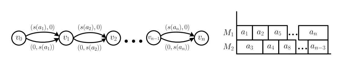
We only need to prove the first part. It is easy to see that the decision version of belongs to NP. Consider an arbitrary instance of partition with with size for each , and let . We now construct the directed graph and the corresponding jobs. The graph has vertices , each pair of is joined by two parallel arcs (jobs) with processing times and respectively, both leading from vertex towards (see the left of Fig. 2). We wish to find the jobs corresponding to a path from to . It is not difficult to check that there is a feasible schedule with makespan not more than if and only if there is a partition of set (see the right of Fig. 2). Therefore, the decision version of is -complete.
4 Approximation Algorithms
4.1 An intuitive Algorithm
To start off, we propose an intuitive algorithm for . The main idea of this algorithm is to set and in , i.e. to find a classical shortest path with one specific set of weights. An intuitive setting is for each arc. We find the shortest path with respect to by Dijkstra’s algorithm, and then schedule the corresponding jobs on the flow shop machines. We refer to this algorithm as the FD algorithm. The subsequent analysis will show that the performance ratio of the FD algorithm remains the same for an arbitrarily selected flow shop scheduling algorithm that provides a dense schedule, regardless of the performance ratio of the algorithm.
It is straightforward that the total running time of the FD algorithm is , where is the running time of the flow shop scheduling algorithm. Therefore, suppose the flow shop scheduling algorithm we used is polynomial time, then the FD algorithm is polynomial time even if is an input of the instance. Before we analyze the performance of this algorithm, we first introduce some notations. Let be the set of jobs in an optimal solution, and be the corresponding makespan, and let and be those returned by the FD algorithm respcetively.
Theorem 4.1
The FD algorithm is -approximate, and this bound is tight.
Proof
Since the returned path is a shortest path with respect to , by (2) we have
| (7) |
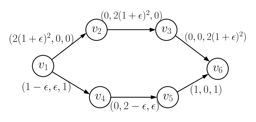
Consider the instance shown in Fig. 3. We wish to find a path from vertex to . The makespan returned by the FD algorithm is with the arc , whereas the makespan of an optimal schedule is with the other arcs. Notice that there is only one job in the returned solution, hence the returned makespan remains regardless of the algorithm used for the flow shop scheduling. The bound is tight because when .
4.2 An Improved Algorithm for Fixed
In this subsection, we assume that , the number of flow shop machines, is a constant. Instead of finding an optimal shortest path from to with respect to specific weights, we implement the ABV algorithm mentioned in Section 2.3, which will return a -approximated solution for the min-max shortest path problem. In other words, we will set and use the objective function in , where the wights will be decided later.
Inspired by the work of Gonzalez and Sahni (1978) and Chen et al. (1996), we proceed as follows: after obtaining a feasible path by the ABV algorithm, we schedule the corresponding jobs by partitioning the machines into several groups. Denote the machine as , (indexed following the routing of the flow shop). More specifically, we partition the machines into groups of three consecutive machines in the routing , , (), groups of two consecutive machines in the routing , (), and individual machines (), in which the value of , , will be derived later. For the three-machine subproblems on , and (), we implement the RS algorithm to obtain the permutations. For the two-machine subproblems on and (), we implement Johnson’s rule to obtain the permutations. The permutations for the single-machine subproblems are arbitrary. Then we form a schedule for the original -machine problem, in which the sequences of jobs on machines are the permutations obtained above, and are executed as early as possible. Notice the property that an optimal schedule is always a permutation schedule only stands for and , and the performance guarantee relies on the properties of critical jobs as we will see in the subsequent analysis. The reason why we partition the machines in this particular fashion is related to this fact, as will be explained below.
The main idea of our algorithm is described as follows. We initially set the weights . The algorithm iteratively runs the ABV algorithm and the above partition scheduling algorithm (the values of will be decided later) by adopting the following revision policy: in a current schedule, if there exists a job whose weight is large enough with respect to the current makespan, we will modify the weights of arcs corresponding to large jobs to , where is a sufficient large number, and then mark these jobs. The algorithm terminates if no such job exists. Another termination condition is that a marked job appears in a current schedule. We return the schedule with minimum makespan among all current schedules as the solution of the algorithm. We refer to this algorithm as the PAR algorithm. Notice that the weights of arcs may vary in each iteration, whereas the processing times of jobs remain the same throughout this algorithm.
Before we formally state the PAR algorithm, we first provide more details about the parameter choices. For and , by following the subsequent analysis of the performance of this algorithm, one can verify that the best possible performance ratio is and respectively. An intuitive argument is that the best possible performance ratio for the general case of the PAR algorithm is . For a given , as are nonnegative integers, our task is to minimize such that . A simple calculation yields the following result:
| (11) |
and
| (15) |
In other words, the best way is to partition the machines in such a way that we have a maximum number of three-machine subsets. The pseudocode of the PAR algorithm is described by Algorithm 4.
It is easy to see that the PAR algorithm will return a feasible solution of . We now discuss its computational complexity. Let the total number of jobs be . Notice that the weights of arcs can be revised at most times. It is straightforward that the total running time of the PAR algorithm is , since there are at most iterations, in which the running time of the ABV algorithm is and scheduling takes time. If and are fixed numbers, then the PAR algorithm is a polynomial time algorithm.
Let be the set of jobs in an optimal solution, and the corresponding makespan, and let and be those returned by the PAR algorithm respectively. The following theorem shows the performance of the PAR algorithm.
Theorem 4.2
Given , the worst-case ratio of the PAR algorithm for is
| (19) |
Proof
We will distinguish two different cases: and .
Case 1
In this case, there is at least one job in the optimal solution, say , such that holds for a current schedule with makespan during the execution. Notice that the schedule returned by the PAR algorithm is the schedule with minimum makespan among all current schedules, and we have . It follows from (3) that
| (20) |
Case 2
Consider the last current schedule during the execution of the algorithm. Denote the corresponding job set and the makespan as and respectively.
In this case, we first argue that . Suppose that this is not the case, i.e. . Since , we know the weights of arcs corresponding to the jobs in have not been revised. Hence we have . Moreover, by the assumption , we have . By Theorem 2.1, the solution returned by the ABV algorithm satisfies
which leads to a contradiction.
Remember that in the PAR algorithm, the machines are divided into three parts, namely three-machines subsets together with at most one two-machine subset or a single machine. We solve these subproblems by the RS algorithm, Johnson’s rule and an arbitrary algorithm respectively. It is clear that the sum of the makespans of those schedules is an upper bound for . Denote and as the makespan and the critical job of the two-machine subproblem returned by Johnson’s rule, and let the corresponding machines be . Denote and , as the makespan and the critical jobs returned by the RS algorithm for the three-machine subproblems with largest makespan, and let the machines be . Denote the single machine as , on which the total processing time is .
For the two-machine case, suppose that . Noticing that for the job scheduled after in the schedule returned by Johnson’s rule and form (5), it follows that
| (21) |
For the three-machine case, we study two subcases corresponding with and for the critical jobs.
Subcase 2.1
.
Consider the schedule with respect to . We can rewrite (4) as
| (22) |
Suppose that the processing times of the critical jobs of the three-machine subproblem satisfy , thus we have , i.e. for the artificial two-machine flow shop in the RS algorithm. Since the RS algorithm schedules the jobs by Johnson’ rule, thus we have for the jobs scheduled after , i.e. . From (22), we have
| (23) |
Since , we know the weights of arcs corresponding to the jobs in the last current schedule have not been revised, and for each job , since otherwise the algorithm will continue. Since , the weights of arcs corresponding to the jobs in this optimal schedule have not been revised. Thus, it follows from (1), (3), Theorem 2.1, (21), (23) and the fact that the schedule returned by the PAR algorithm is the schedule with minimum makespan among all current schedules, that
Subcase 2.2
.
We also assume that , and , an argument similar to the previous case shows that the jobs scheduled after satisfies . Since , it follows from (4) that
| (25) |
Similarly, it is not difficult to show that
For the cases where the last current schedule has critical jobs satisfying or , analogous arguments would yield the same result.
Now we show that the performance ratio of the PAR algorithm cannot less than . First, we propose two instances for and .
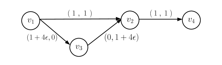
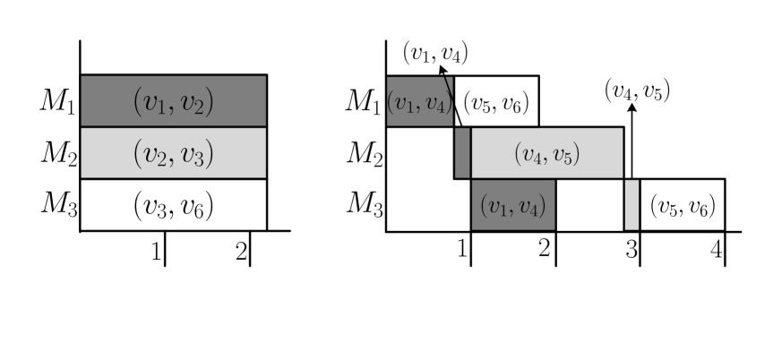
If , the performance ratio of the PAR algorithm is . Consider the following instance shown in Fig. 4. We wish to find a path from to . Notice that the ABV algorithm returns the path with arcs and , and the corresponding makespan by Johnson’s rule is . All the corresponding jobs satisfy , and thus the algorithm terminates. Therefore, the makespan of the returned schedule by the PAR algorithm is (see the right schedule of Fig. 4). On the other hand, the optimal makespan is with arcs , and (see the left schedule of Fig. 4). The worst case ratio of the PAR algorithm cannot be less than as when for this instance.
For the case where , the performance ratio of the PAR algorithm is . Consider the instance shown in Fig. 5. We wish to find a path from vertex to . Notice that the ABV algorithm returns the path with arcs . The makespan of the schedule returned by the RS algorithm is . All the corresponding jobs satisfy , and thus the algorithm terminates. Therefore, the makespan of the schedule returned by the PAR algorithm is (see the right schedule of Fig. 5). On the other hand, the makespan of an optimal job schedule is , by selecting the arcs , , and (see the left schedule of Fig. 5). The worst case ratio of the PAR algorithm cannot be less than as when for this instance.
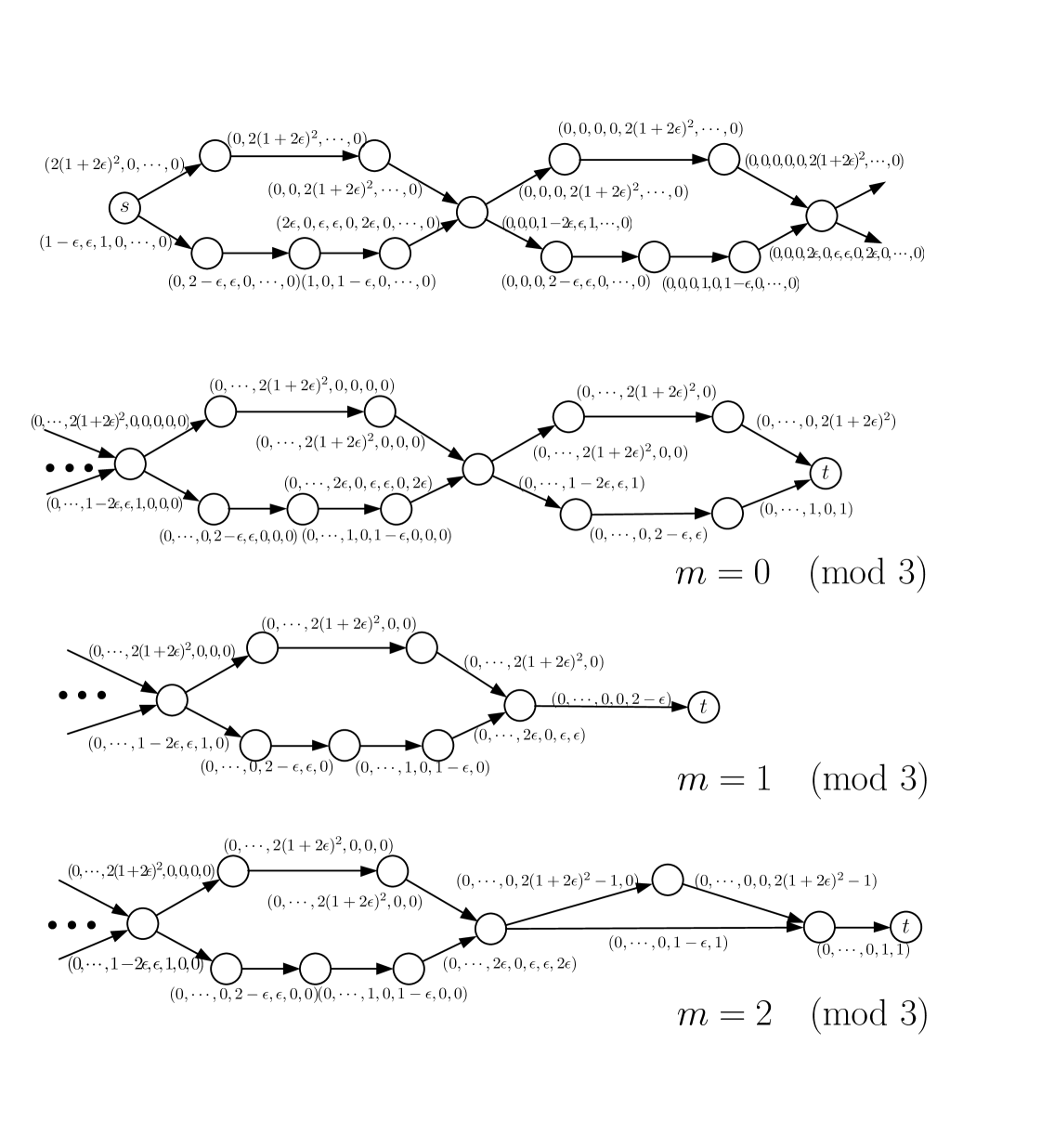
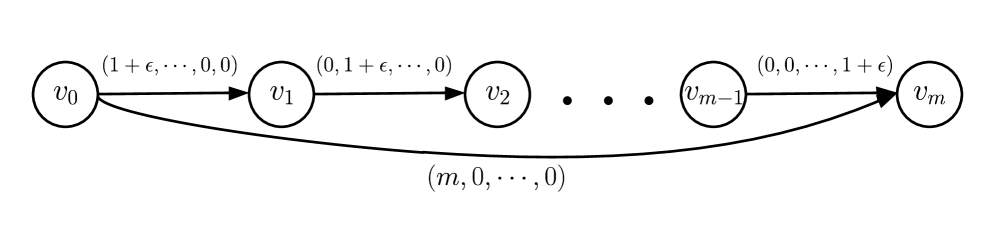
By extending and modifying the above examples to the general case, the instance described in Fig. 6 can be used to show that the performance ratio of the PAR algorithm cannot be less than .
5 Conclusions
This paper has studied a combination problem of flow shop scheduling and the shortest path problem. We show the hardness of this problem, and present some approximation algorithms. For future research, it would be interesting to find an approximation algorithm with a better performance ratio for this problem. The question whether is NP-hard in the strong sense is still open. One can also consider the combination of other combinatorial optimization problems. All these questions deserve further investigation.
Acknowledgments
This work has been supported by the Bilateral Scientific Cooperation Project BIL10/10 between Tsinghua University and KU Leuven.
References
- Ahuja et al. (1993) Ahuja RK, Magnanti TL, Orlin JB (1993) Network Flows: Theory, Algorithms, and Applications. Prentice Hall, New Jersey
- Aissi, Bazgan and Vanderpooten (2006) Aissi H, Bazgan C, Vanderpooten D (2006) Approximating min-max (regret) versions of some polynomial problems. In: Chen, D., Pardolos, P.M. (eds.) COCOON 2006, LNCS, vol 4112, pp 428–438. Springer, Heidelberg
- Batagelj et al. (2000) Batagelj V, Brandenburg FJ, Mendez P, Sen A (2000) The generalized shortest path problem. CiteSeer Archives
- Bodlaender et al. (1994) Bodlaender HL, Jansen K, Woeginger GJ (1994) Scheduling with incompatible jobs. Disc Appl Math, 55: 219–232
- Chen et al. (1996) Chen B, Glass CA, Potts CN, Strusevich VA (1996) A new heuristic for three-machine flow shop scheduling. Oper Res 44: 891–898
- Conway et al. (1971) Conway RW, Maxwell W, Miller L (1967) Theory of scheduling. Reading
- Dijkstra (1959) Dijkstra EW (1959) A note on two problems in connexion with graphs. Numer Math 1: 269–271
- Garey et al. (1976) Garey MR, Johnson DS, Sethi R (1976) The complexity of flowshop and jobshop scheduling. Math Oper Res 1: 117–129
- Garey and Johnson (1979) Garey MR, Johnson DS (1979) Computers and Intractability: A Guide to the Theory of NP-completeness. Freeman, San Francisco
- Gonzalez and Sahni (1978) Gonzalez T, Sahni S (1978) Flowshop and jobshop schedules: complexity and approximation. Oper Res 26: 36–52
- Hall (1988) Hall LA (1998) Approximability of flow shop scheduling. Math Program 82: 175–190
- Johnson (1954) Johnson SM (1954) Optimal two- and three-stage production schedules with setup times included. Nav Res Logist Q 1: 61–68
- Kouvelis and Yu (1997) Kouvelis P, Yu G (1997) Robust discrete optimization and its applications. Kluwer Academic Publishers, Boston
- Röck and Schmidt (1982) Röck H, Schmidt G (1982) Machine aggregation heuristics in shop scheduling. Method Oper Res 45: 303–314
- Wang and Cui (2012) Wang Z, Cui Z (2012) Combination of parallel machine scheduling and vertex cover. Theor Comput Sci 460: 10–15
- Wang et al. (2013) Wang Z, Hong W, He D (2013): Combination of parallel machine scheduling and covering problem. Working paper, Tsinghua University
- Warburton (1987) Warburton A (1987) Approximation of pareto optima in multiple-objective, shortest-path problems. Oper Res 35: 70–79