A common trajectory recapitulated by urban economies
Abstract
Is there a general economic pathway recapitulated by individual cities over and over? Identifying such evolution structure, if any, would inform models for the assessment, maintenance, and forecasting of urban sustainability and economic success as a quantitative baseline. This premise seems to contradict the existing body of empirical evidences for path-dependent growth shaping the unique history of individual cities. And yet, recent empirical evidences and theoretical models have amounted to the universal patterns, mostly size-dependent, thereby expressing many of urban quantities as a set of simple scaling laws. Here, we provide a mathematical framework to integrate repeated cross-sectional data, each of which freezes in time dimension, into a frame of reference for longitudinal evolution of individual cities in time. Using data of over 100 millions employment in thousand business categories between 1998 and 2013, we decompose each city’s evolution into a pre-factor and relative changes to eliminate national and global effects. In this way, we show the longitudinal dynamics of individual cities recapitulate the observed cross-sectional regularity. Larger cities are not only scaled-up versions of their smaller peers but also of their past. In addition, our model shows that both specialization and diversification are attributed to the distribution of industry’s scaling exponents, resulting a critical population of 1.2 million at which a city makes an industrial transition into innovative economies.
For societies worldwide, large cities play an important role in economic productivity and innovation Glaeser et al. (1992); Quigley (1998). The resulting economic and social opportunities drive worker migration to cities, thus producing an era of accelerated urban growth International Organization for Migration (2015); Rozenblat and Pumain (2007) and the advent of “megacities” Dobbs (2010). Therefore, policy makers in growing cities must identify and leverage any available insight into the sustainability and future development of their local economies.
Specialization, a centerpiece of urban growth and change, has long been the virtue of urban development, shaping culturally and economically every city’s idiosyncratic path-dependent trajectory. The prominence of urban economies are characterized, and hence understood by distinctive socio-economic activities, mainly in a form of specialization Henderson (1991); Duranton and Puga (2000). This specialized urban development is considered as a result of a bundle of available natural resources Ellison and Glaeser (1997, 1999), a cluster of geographic advantages Porter (1997); Delgado et al. (2014); Glaeser (2005a), a sequence of strategic decisions Markusen (1996); Evans (2009); Storper et al. (2015), or a series of historical contingencies Henderson (1991); Martin and Sunley (2006); Glaeser (2005b). Therefore, studies often choose one or two cities of interest, and describe and explain their distinctive trajectories of economic development focusing one or more of the factors above (e.g. New York Glaeser (2005a), Boston Glaeser (2005b), Los Angeles and San Francisco Storper et al. (2015)). These individual trajectories are observed to diverge rather than converge to a single path Markusen and Schrock (2006); Turok (2009), and such details are difficult to perform for all US cities in a comparative way.
In the presence of path-dependent specialization, the very existence of general patterns across cities is puzzling. These regularities include the famous Zipf’s law, urban scaling, the number-size rule, and the universal distribution and hierarchical structure of business, which are largely expressed as a function of city size Bettencourt et al. (2007); Batty (2008, 2013); Barthélemy (2011); Bettencourt et al. (2010); Gomez-Lievano et al. (2016); Schiller (2016); Zipf (1949); Fujita et al. (1999); Mori et al. (2008); Bettencourt (2013); Youn et al. (2016). Indeed, population size has been a great indicator of many of urban properties, among which we are particularly interested in the industrial composition. For example, small cities heavily rely on manufacturing-based labor while large cities on cognitive labor Henderson (1986); Florida (2004); Michaels et al. (2013); Youn et al. (2016); Frank et al. (2018).
These regularities have served as an excellent reference point for urban growth model, but they are nonetheless cross-sectional, freeze in time. To what extent do these cross-sectional regularities embody the longitudinal trajectories of individual cities? It is conceivable that the common hierarchical structure, inside and across cities, results self-similar growth in time, also manifested as cross-sectional regularities Christaller (1933); Fujita et al. (1999); Lee et al. (2017). The general economic development, largely observed at the national level, may be recapitulated by individual cities Hidalgo et al. (2007); Hidalgo and Hausmann (2009); Thurner et al. (2010); Klimek et al. (2012); Shutters et al. (2016); Sachs and Warner (1995). Identifying such underlying structure will make a better predictive model for growing cities, and thus help urban policy makers to assess developmental opportunities.
In this study, we analyze the economic activities in U.S. cities between 1998 and 2013. First, we demonstrate that population size determines the industrial composition in a city. We then quantify to what extent this cross-sectional regularity is recapitulated by individual cities’ longitudinal dynamics. Finally, we show how cities make transition between the manufacturing economy to the productive and innovative economy, and analytically derive the transition population.
Results
Characteristic Industries Determined by City Size
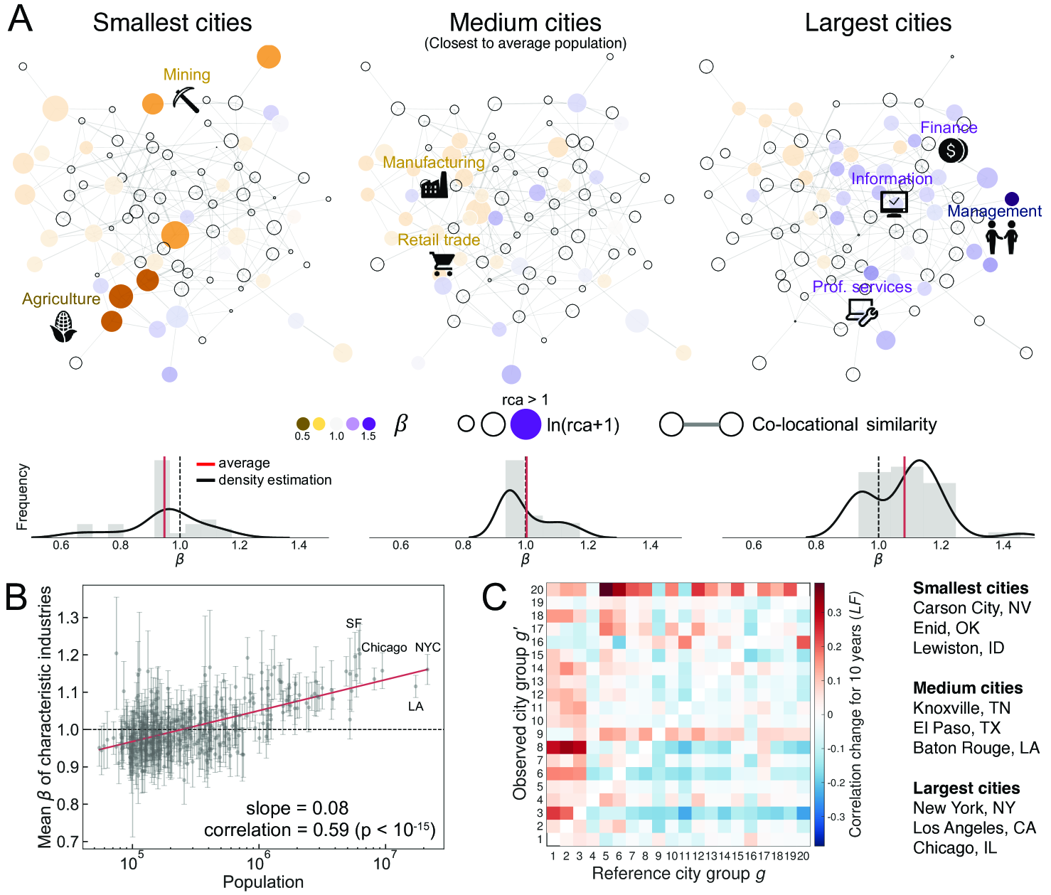
We characterize the economies of 350 U.S. cities between 1998 and 2013 by industries’ relative size using the North American Industry Classification System (NAICS) (see Materials and Methods and SI. I for full description on data). Revealed Comparative Advantage (RCA), also known as location quotient, is a widely used measure for a region’s industrial specialization Hidalgo et al. (2007); Isserman (1977); Glaeser et al. (1992); Markusen and Schrock (2006). It is the city’s relative employment share to the national average for the industry , and we define characteristic industry if its share in city is greater than national level at time , (solid color in Fig. 1A) Balassa (1965); Hidalgo et al. (2007).
Scaling theory remains as a powerful framework for size-dependent nature of urban characteristics Bettencourt et al. (2007); Youn et al. (2016); Bettencourt and Lobo (2016); Gomez-Lievano et al. (2016) and dynamics Bettencourt et al. (2010); Alves et al. (2015) despite its statistical caveat Arcaute et al. (2015); Leitao et al. (2016). Urban quantities are expressed as
| (1) |
where pre-factor and scaling exponent are fitted given empirical observations of employment and population . We find the Eq. 1 is mostly in a good agreement with our dataset (, see SI. III). Then, characterizes the size-dependency of industry (sublinear, linear and superlinear).
Figure 1 summarizes our analyses in a network representation where characteristic industries are colored by and sized by RCA. Two industry and are connected by co-occurrence similarity, across US cities (see Materials and Methods) Hidalgo et al. (2007); Neffke and Svensson Henning (2008); Muneepeerakul et al. (2013); Shutters et al. (2016). As population grows, where the city’s characteristic industries occupying in the network moves (from agriculture and mining to managerial and technology-based industries), and this transition seems to be predicted by scaling exponents Youn et al. (2016).
City size determines what are the characteristic industries and their directions are manifested as scaling exponents. For example, small cities are characterized by sublinear industries (), such as agriculture and mining, while large cities are by superlinear industries () such as management and professional services. This result is consistent with existing observations that small cities are relying more on manual labor Henderson (1986) while large cities on cognitive labor Michaels et al. (2013); Florida (2004); Youn et al. (2016), suggesting an industrial transition according to from sublinear to superlinear sectors (see Fig. 1A). Fig. 1B confirms this overall trend at the level of individual U.S. cities. The average scaling exponent for the characteristic industries in each city is strongly correlated with population size (Pearson correlation ).
Lead-Follow Matrix
So far, our analysis uses a static snapshot of urban economies, but how do these cross-sectional relationships relate to temporal change in cities? Here, we explore urban recapitulation through the industrial composition of different sized cities over time. Cities are grouped into 20 equally-populated city groups (denoted by ) according to city size, and we represent the industrial characteristic of group as industry vector composed of logarithmic RCA values averaged for cities in group (see Materials and Methods). Then, the Pearson correlations of and describes how the industrial compositions of city groups and relate over different time periods and . A lead-follow score aggregates these industrial changes over each starting year in our data set, according to
| (2) |
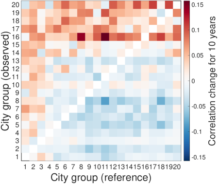
This score is basically the average similarity change between reference group and observed group over a 10 year period as default, and a lead-follow matrix for the scores of all pairs summarizes the overall trend (see SI. IV for other time periods).
The resulting lead-follow matrix provides temporal evidence for urban recapitulation (see Fig. 1C). Groups of small cities become more similar to groups of large cities over a ten year period while groups of large cities become increasingly dissimilar to groups of small cities. This observation suggests that there exists a general pathway explored by large cities and followed by small cities over time. We interpret the lead-follow matrix as strong evidence for urban recapitulation of industrial compositions, and we endeavor to explain the phenomenon further. City size determines both characteristic industries therein and the future growth.
Explaining Urban Recapitulation
How does city size characterize urban economic structures and their dynamics? Characterized industries are determined by city size and scaling exponents. First, revealed comparative advantage of city is expressed as an industry’s relative size to a national level. The industry’s size is explained by scaling relation Eq. 1. Therefore, we can express RCA as a function of scaling exponents as following:
| (3) |
The equation can be further approximated by Zipf’s law Rosen and Resnick (1980) (see SI. V):
| (4) |
where and are size of the largest and smallest city at time , respectively (see SI. V for a complete derivation).
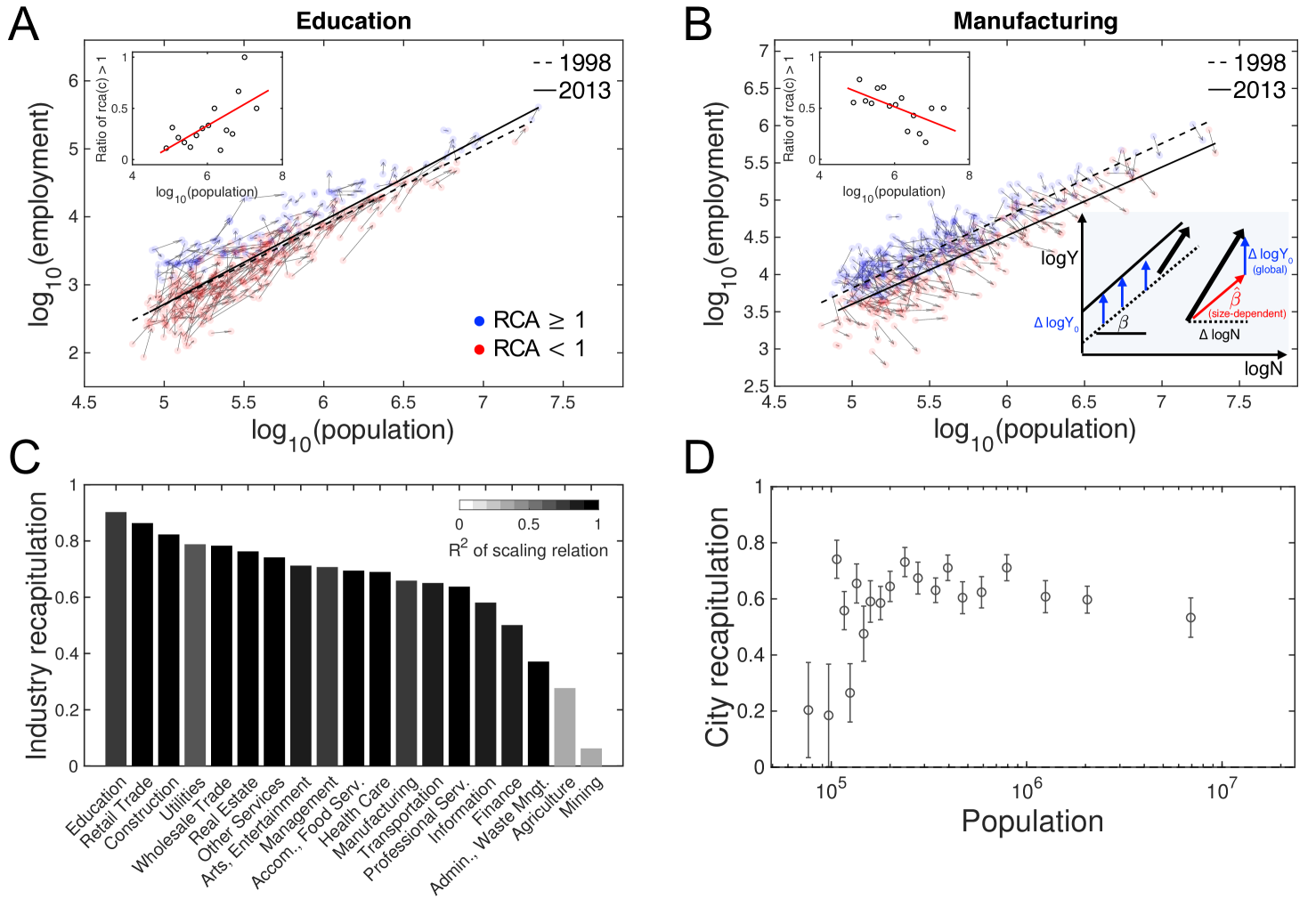
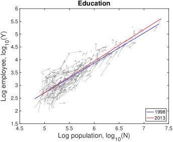
This framework determines the characteristic industries and predicts which industry will be characteristic given scaling relations. When cities grow, superlinear industries, , will be characteristic industries as a result of increasing RCA value, as shown in Fig. 1A&B. We exemplify this observation empirically by examining the growth of individual U.S. cities from 1998 to 2013 compared to their RCA values for the Education industry (see Fig. 2A), which has , and the Manufacturing industry (see Fig. 2B), which has .
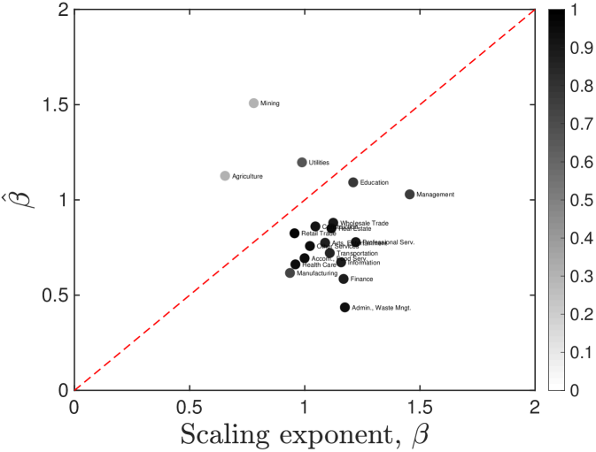
Both our analytic framework and empirical observations imply the existence of urban recapitulation by city size. Now, how can we measure the degree of recapitulation for individual industries and cities? The size-dependency estimates the employment growth when the population grows in time. We compare the cross-sectional ratio and the observed longitudinal growth ratio as a measure of recapitulation. From Eq. 1, we have
| (5) |
where , and the same for and . This calculation decomposes employment growth into each city’s size-dependent growth (i.e. ) and global time-dependent growth (i.e. . See the schematic in Fig. 2B). By fitting Eq. 5 to empirical employment data, we derive the longitudinal size-dependency and the global trend across all cities between 1998 and 2013, and we compare with the cross-sectional size-dependency . If an individual industry is perfectly recapitulated by growing cities, then cross-sectional and longitudinal size-dependencies should be equal (). Therefore, we employ an industry recapitulation score according to
| (6) |
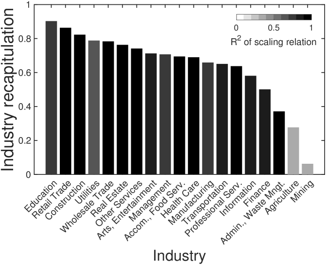
The industry recapitulation score becomes one when every city perfectly recapitulates, and equals to zero when employment growth has no longitudinal size-dependency.
We observe high recapitulation scores (i.e. ) for industries that are well-described by urban scaling (i.e. ). This strong longitudinal size-dependency is a sufficient condition of the constant deviation from a common trajectory Bettencourt et al. (2010). In contrast to the recent research on traffic congestion Depersin and Barthelemy (2018), the common trajectory is well explained by city size. The most significant difference is teasing out the global trend, , which makes common upward or downward drifts as shown in manufacturing in Fig. 2B. Its recapitulation score around shows that decomposition is essential to properly measure the size-dependent growth.
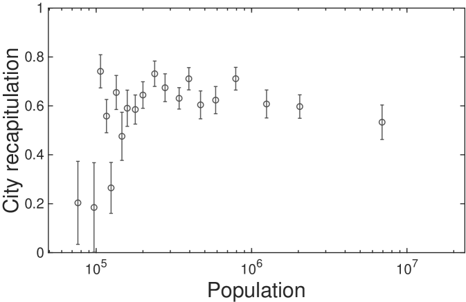
Analogous to industries, do cities recapitulate with the same strength? We generalize the decomposition in Eq. 5 for individual cities, and measure the recapitulation scores of city groups, accordingly. We extract the size-dependent growth of each city by subtracting the global growth estimated from Eq. 5. Then, we measure the longitudinal size-dependency averaged for the cities in city group and industry similar to (see SI. VI for the details).
| (7) |
where is the set of cities in city group , and the groups are determined in the order of populations. Finally, we measure a city group recapitulation score according to
| (8) |
where is the set of all industries. Similar to before, larger values of mean large tendency of recapitulation.
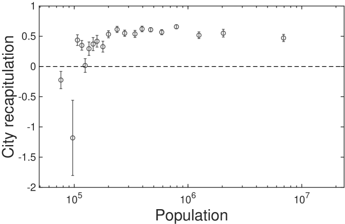
In addition to industries, a strong tendency of recapitulation is also observed for city groups. Fig. 2D demonstrates that recapitulation occurs across all city groups as . Most city groups exhibit a high strength of recapitulation, except for a few groups of very small cities. From the measured recapitulation scores of industries and cities, we conclude that cities recapitulate a general pathway ruled by city size, in agreement with the observed lead-follow matrix and our framework connecting RCA and scaling relation.
Transition into Innovative Economies
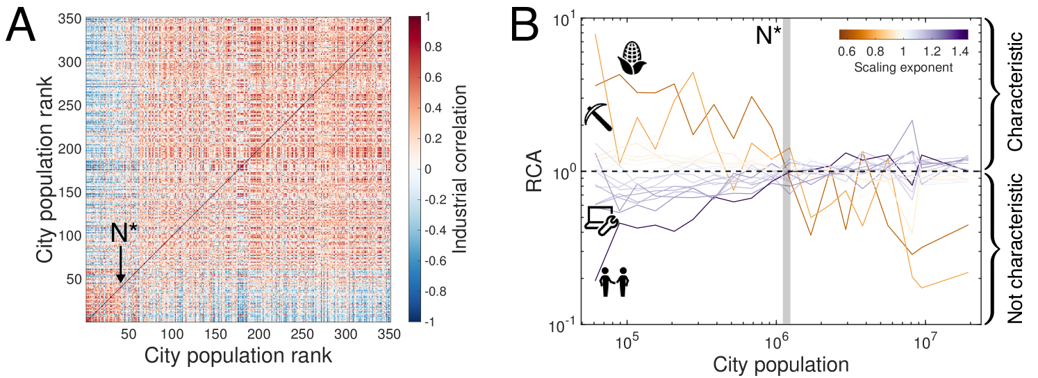
The observed recapitulation predicts the structural change of urban economy, represented by characteristic industries, as city size grows. Can we specify the characteristic size at which a city transitions from a small city economy into the innovative and productive economy of large cities? Specifically, given the analytical relationship between city size and corresponding characteristic industries in Eq. 4, at what size do cities begin to leverage innovative industries Youn et al. (2016) with ? Fig. 3A compares cities according to size and the Pearson correlation of logarithmic RCA values (i.e. ) for city pairs averaged for entire time span. We observe a transition at around the 50th largest city indicating that the 50 largest cities are characterized by qualitatively different industries compared to the remaining smaller cities.
Our framework can explain this observed transition through a fixed point in the plane. From Eq. 4, we observe a saddle point at and city size million, which is around the population of Louisville, KY, the 43rd largest city (see SI. V for a complete derivation). The existence of this fixed point suggests that characteristic industries in growing cities will change based on as cities achieve this critical size. We expect that small cities with will be characterized by industries with while large cities with will be characterized by industries with . Fig. 3B empirically confirms that scaling exponents distinguish the trends of characteristic industries by city size. The characteristic industries of growing cities transition from industries with to industries with at precisely the predicted city size 1.2 millions.
Discussion
We provide a comprehensive framework that connects the cross-sectional size-dependency of urban economies to longitudinal industrial composition in US cities in a process that well-described as “urban recapitulation.” We provide both analytical and empirical evidence to support the existence of a common trajectory that cities grow along. Our observations show that urban economies actually recapitulate a common trajectory at an aggregate level, which anticipates economic change as cities grow.
Surprisingly, our recapitulation framework identifies industrial transitions at population size of 1.2 million where the increasing prominence with population of superlinearly-scaled industries crosses the decreasing trend of sublinearly-scaled industries. It shows good agreement with empirical results that superlinearly-scaled industries are characteristic in large cities while sublinearly-scaled industries are characteristic in small cities. Scaling exponents are often considered as a proxy of innovation and maturity, as primary and secondary sectors have sublinear scaling, while managerial and professional industries have superlinear scaling Pumain et al. (2006); Youn et al. (2016). Therefore, an urban economy is expected to become more innovative, creative, and economically desirable as the city grows above some characteristic size. This result informs policy makers, employers and job-seekers about upcoming structural changes in the local labor market.
At first, our finding seems to contrast the conventional wisdom in urban studies that suggests cities possess unique individual trajectories Markusen and Schrock (2006); Turok (2009). However, this specialization is also explained by the recapitulation framework. A specialized city is represented by only a small number of characteristic industries, and we showed that superlinearity and sublinearity distinguish characteristic industries in small and large cities. Therefore, the specialization trend in size is determined by the number of sublinearly- and superlinearly-scaled industries. In our case, the small number of sublinearly-scaled industries results in higher specialization in small cities (see Fig. S9). Specialization is not a random accident or localized feature, but a regular characteristic. Distinctive pathways of individual cities are also understood by the recapitulation framework as population growth differentiates industrial growth according to their scaling exponents. We can regard the deviation from the common trajectory as an effective distinctive pathway Bettencourt et al. (2010). This enables us to measure distinctiveness more accurately, and hence our analysis may contribute to a well-individualized urban policy Turok (2009).
In the previous studies on clusters of traded industries Porter (2003) and national exports Hidalgo et al. (2007), economic characteristics and their growth are considered as independent of population size. Then, why do we observe strong recapitulation by city size? Most of these studies looked into tradeable sectors and exclude production and consumption in domestic market. As a result, they overstate their comparative advantages because they sell products in external markets. By considering both internal external production and consumption, our results show different level of recapitulation by tradeability. We observe strong recapitulation in the industries that we locally consume, such as education, retail trade, construction, and utility, while weak recapitulation in tradaeble industries, such as agriculture, mining, administrative service, and finance. Our analysis provides a reliable reference for economic growth by tradeability.
Economic output is often expressed as a product function of labor and capital inputs, which are implicit functions of population Lobo et al. (2013). Our approach turns around this convention by bringing this implicit relation to an explicit functional form and isolating industry’s size-dependent growth in urban areas from any other factors. Individuals make up a city and account for socio-economic activities that constitute labor and result in capital, the product of which becomes the economic output. Thus, we consider population as a fundamental unit to make a first-order approach to the economic output. Indeed, there are numerous higher-order attributes unexplained by population: available natural resources, accessibility, and economic intervention Ellison and Glaeser (1997, 1999). In addition, not every industry perfectly fits to a scaling function, and yet the functional form serves well to derive a general characteristics of recapitulation and industrial transition at Arcaute et al. (2015); Leitao et al. (2016).
Our framework is inspired by the recapitulation theory in biology Ehrlich and Holm (1963) much the same as urban scaling theory Bettencourt et al. (2007) is motivated from the allometric scaling in biology West et al. (1997). However, there is a conceptual difference between them. In biological recapitulation, close species grow on a common pathway as they recapitulate a shared evolutionary pathway composed of many common ancestors. We consider each city as a footprint of evolutionary pathway of the largest city, thus, we regard the scaling relation itself as the common trajectory. Although cities have followed the general pathway in our short-term data, our framework needs to be evaluated and advanced through further works on long-term data Pumain et al. (2006).
Employing the scaling framework, we have discussed several urban economic characteristics: recapitulation, transition, specialization and distinctiveness. Unveiling the origin of urban scaling will answer how urban economies have evolved with embodying such characteristics. While there are several reliable explanations using networks Bettencourt (2013), necessary complementary factors Gomez-Lievano et al. (2016), collective brains Kline and Boyd (2010); Muthukrishna and Henrich (2016) and social interactions Yang et al. (2017), we still lack a concrete generative mechanism and its empirical confirmation to explain how microlevel individual capabilities aggregate into collective intelligence, and then manifest economic outputs formulated as scaling relations. Identifying such mechanism will specify insufficient capabilities for growth and enable urban policy makers to build an appropriate policy for sustainable economic success.
Materials and Methods
Data
This study uses employment data by North American Industry Classification System (NAICS) industry code and 350 U.S. metropolitan statistical areas (referred to as “city” throughout the manuscript) according to the U.S. Bureau of Labor Statistics. The sizes of industry set are 19, 86, 289, 642 and 978 according to the depth of classification denoted by 2-6 digits. Data includes annual employment measurements for the years 1998 through 2013.
Identifying Characteristic Industries with RCA
We employ revealed comparative advantage (RCA) Balassa (1965); Hidalgo et al. (2007) to identify characteristic industries in each U.S. city. Let denote the set of 2-digits NAICS industry codes and denote the set of U.S. cities, then denotes the employment in industry in city at year . The revealed comparative advantage is given by
| (9) |
where , and denote city, industry and time, respectively.
We can characterize industry as a vector of RCA values of cities as . The time-averaged inter-industry relatedness is defined by the Pearson correlation of two industry vectors and as
| (10) |
where is the Pearson correlation function. Figure 1 A shows links that satisfy .
Lead-Follow Relationship
In the analysis on lead-follow relationship, we bin cities into 20 equally-populated city groups (denoted by ) according to city size, and, for each city group, we calculate the average RCA values of each city according to
| (11) |
where denotes the set of 2-digit NAICS industry codes.
Acknowledgements.
The authors thank to Ricardo Hausmann, Frank Neffke, Luís M. A. Bettencourt and César Hidalgo for useful comments. W.-S. Jung was supported by Basic Science Research Program through the National Research Foundation of Korea (NRF) funded by the Ministry of Education (2016R1D1A1B03932590).References
- Glaeser et al. (1992) E. L. Glaeser, H. D. Kallal, J. A. Scheinkman, and A. Shleifer, Journal of political economy 100, 1126 (1992).
- Quigley (1998) J. M. Quigley, The Journal of Economic Perspectives 12, 127 (1998).
- International Organization for Migration (2015) International Organization for Migration, World Migration Report 2015 - Migrants and Cities: New Partnerships to Manage Mobility, Tech. Rep. (2015).
- Rozenblat and Pumain (2007) C. Rozenblat and D. Pumain, in Cities in Globalization: Practices, Policies, and Theories (Routledge, 2007) pp. 130–156.
- Dobbs (2010) R. Dobbs, Foreign Policy Magazine 181, 132 (2010).
- Henderson (1991) J. V. Henderson, Urban Development: Theory, Fact, and Illusion, OUP Catalogue (Oxford University Press, 1991).
- Duranton and Puga (2000) G. Duranton and D. Puga, Urban studies 37, 533 (2000).
- Ellison and Glaeser (1997) G. Ellison and E. L. Glaeser, Journal of political economy 105, 889 (1997).
- Ellison and Glaeser (1999) G. Ellison and E. L. Glaeser, American Economic Review 89, 311 (1999).
- Porter (1997) M. E. Porter, Economic Development Quarterly 11, 11 (1997).
- Delgado et al. (2014) M. Delgado, M. E. Porter, and S. Stern, Research Policy 43, 1785 (2014).
- Glaeser (2005a) E. L. Glaeser, Urban colossus: why is New York America’s largest city?, Tech. Rep. (National Bureau of Economic Research, 2005).
- Markusen (1996) A. Markusen, International Regional Science Review 19, 49 (1996).
- Evans (2009) G. Evans, Urban studies 46, 1003 (2009).
- Storper et al. (2015) M. Storper, T. Kemeny, N. Makarem, and T. Osman, The rise and fall of urban economies: Lessons from San Francisco and Los Angeles (Stanford University Press, 2015).
- Martin and Sunley (2006) R. Martin and P. Sunley, Journal of economic geography 6, 395 (2006).
- Glaeser (2005b) E. L. Glaeser, Journal of Economic Geography 5, 119 (2005b).
- Markusen and Schrock (2006) A. Markusen and G. Schrock, Urban studies 43, 1301 (2006).
- Turok (2009) I. Turok, Environment and planning A 41, 13 (2009).
- Bettencourt et al. (2007) L. M. A. Bettencourt, J. Lobo, D. Helbing, C. Kühnert, and G. B. West, PNAS 104, 7301 (2007).
- Batty (2008) M. Batty, Science 319, 769 (2008).
- Batty (2013) M. Batty, The new science of cities (Mit Press, 2013).
- Barthélemy (2011) M. Barthélemy, Physics Reports 499, 1 (2011).
- Bettencourt et al. (2010) L. M. A. Bettencourt, J. Lobo, D. Strumsky, and G. B. West, PloS one 5, e13541 (2010).
- Gomez-Lievano et al. (2016) A. Gomez-Lievano, O. Patterson-Lomba, and R. Hausmann, Nature Human Behaviour 1, 0012 (2016).
- Schiller (2016) F. Schiller, Journal of Cleaner Production 112, 4273 (2016).
- Zipf (1949) G. K. Zipf, Human Behavior and the Principle of Least Effort (Addison-Wesley, 1949).
- Fujita et al. (1999) M. Fujita, P. Krugman, and T. Mori, European Economic Review 43, 209 (1999).
- Mori et al. (2008) T. Mori, K. Nishikimi, and T. E. Smith, Journal of Regional Science 48, 165 (2008).
- Bettencourt (2013) L. M. A. Bettencourt, Science 340, 1438 (2013).
- Youn et al. (2016) H. Youn, L. M. A. Bettencourt, J. Lobo, D. Strumsky, H. Samaniego, and G. B. West, Journal of The Royal Society Interface 13, 20150937 (2016).
- Henderson (1986) J. V. Henderson, Journal of Urban economics 19, 47 (1986).
- Florida (2004) R. Florida, The rise of the creative class (Basic books New York, 2004).
- Michaels et al. (2013) G. Michaels, F. Rauch, and S. J. Redding, Task specialization in US cities from 1880-2000, Tech. Rep. (National Bureau of Economic Research, 2013).
- Frank et al. (2018) M. R. Frank, L. Sun, M. Cebrian, H. Youn, and I. Rahwan, Journal of The Royal Society Interface 15 (2018), 10.1098/rsif.2017.0946.
- Christaller (1933) W. Christaller, “Die zentralen orte in süddeutschland, jena: Gustaf fisher. translated by carlisle w. baskin (1966), as central places in southern germany,” (1933).
- Lee et al. (2017) M. Lee, H. Barbosa, H. Youn, P. Holme, and G. Ghoshal, Nature Communications 8 (2017), 10.1038/s41467-017-02374-7.
- Hidalgo et al. (2007) C. A. Hidalgo, B. Klinger, A.-L. Barabási, and R. Hausmann, Science 317, 482 (2007).
- Hidalgo and Hausmann (2009) C. A. Hidalgo and R. Hausmann, PNAS 106, 10570 (2009).
- Thurner et al. (2010) S. Thurner, P. Klimek, and R. Hanel, New Journal of Physics 12, 075029 (2010).
- Klimek et al. (2012) P. Klimek, R. Hausmann, and S. Thurner, PloS one 7, e38924 (2012).
- Shutters et al. (2016) S. T. Shutters, R. Muneepeerakul, and J. Lobo, Urban Studies 53, 3439 (2016).
- Sachs and Warner (1995) J. D. Sachs and A. M. Warner, Economic convergence and economic policies, Tech. Rep. (National Bureau of Economic Research, 1995).
- Isserman (1977) A. M. Isserman, Journal of the American Institute of Planners 43, 33 (1977).
- Balassa (1965) B. Balassa, The Manchester School 33, 99 (1965).
- Bettencourt and Lobo (2016) L. M. A. Bettencourt and J. Lobo, Journal of The Royal Society Interface 13, 20160005 (2016).
- Alves et al. (2015) L. G. Alves, R. S. Mendes, E. K. Lenzi, and H. V. Ribeiro, PloS one 10, e0134862 (2015).
- Arcaute et al. (2015) E. Arcaute, E. Hatna, P. Ferguson, H. Youn, A. Johansson, and M. Batty, Journal of The Royal Society Interface 12, 20140745 (2015).
- Leitao et al. (2016) J. C. Leitao, J. M. Miotto, M. Gerlach, and E. G. Altmann, Royal Society open science 3, 150649 (2016).
- Neffke and Svensson Henning (2008) F. Neffke and M. Svensson Henning, Papers in Evolutionary Economic Geography 8, 19 (2008).
- Muneepeerakul et al. (2013) R. Muneepeerakul, J. Lobo, S. T. Shutters, A. Goméz-Liévano, and M. R. Qubbaj, PLoS ONE 8, e73676 (2013).
- Rosen and Resnick (1980) K. T. Rosen and M. Resnick, Journal of Urban Economics 8, 165 (1980).
- Depersin and Barthelemy (2018) J. Depersin and M. Barthelemy, Proceedings of the National Academy of Sciences 115, 2317 (2018).
- Pumain et al. (2006) D. Pumain, F. Paulus, C. Vacchiani-Marcuzzo, and J. Lobo, Cybergeo : European Journal of Geography (2006), 10.4000/cybergeo.2519.
- Porter (2003) M. Porter, Regional studies 37, 549 (2003).
- Lobo et al. (2013) J. Lobo, L. M. A. Bettencourt, D. Strumsky, and G. B. West, PLoS One 8, e58407 (2013).
- Ehrlich and Holm (1963) P. R. Ehrlich and R. W. Holm, The process of evolution, Tech. Rep. (1963).
- West et al. (1997) G. B. West, J. H. Brown, and B. J. Enquist, Science 276, 122 (1997).
- Kline and Boyd (2010) M. A. Kline and R. Boyd, Proceedings of the Royal Society of London B: Biological Sciences 277, 2559 (2010).
- Muthukrishna and Henrich (2016) M. Muthukrishna and J. Henrich, Phil. Trans. R. Soc. B 371, 20150192 (2016).
- Yang et al. (2017) V. C. Yang, A. V. Papachristos, and D. M. Abrams, arXiv preprint arXiv:1712.00476 (2017).
- Vollrath (1991) T. L. Vollrath, Review of World Economics 127, 265 (1991).
- Gao et al. (2017) J. Gao, B. Jun, A. Pentland, T. Zhou, C. A. Hidalgo, et al., arXiv preprint arXiv:1703.01369 (2017).
Supporting Information: A common trajectory recapitulated by urban economies
I Datasets
A
B
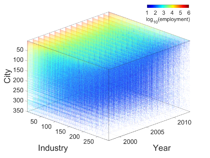
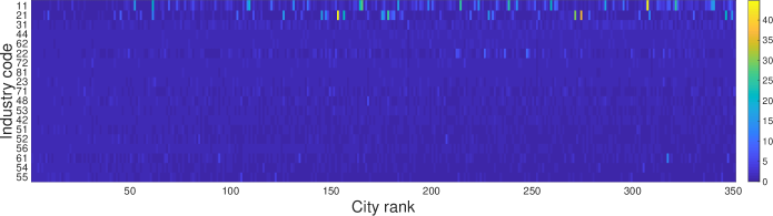
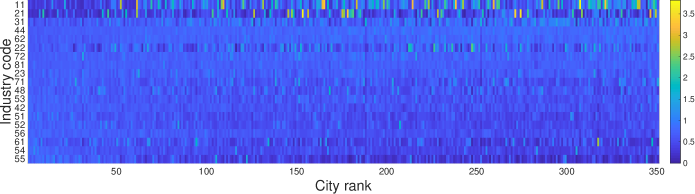
We study the dynamics and structure of urban industries using 16-years of employment and establishment data from 1998 to 2013 provided by the County Business Patterns (CBP). The number of industry sectors differs for classification levels from 19 to 978 by North American Industry Classification System (NAICS). We use 350 Metropolitan Statistical Areas (MSAs) as a definition of cities with their yearly populations; this data is provided by the U.S. Census Bureau. We use to denote the size of industry in city at time , and we use to denote the city’s population.
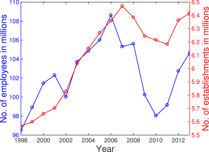
An aggregate spatio-temporal view of the complete data set is provided in Figure S1A. Large cities have a larger number of industries than small cities. Figure S1B depicts the time series of the total number of employees and establishments across all U.S. cities. The temporal changes of employees and establishments show a similar trend which includes a trough near 2010. The number of employees in some industries is denoted as size classes because the data need to avoid disclosure (confidentiality) or they do not meet publication standards. The employee size classes are as follows: A for 0-19, B for 20-99, C for 100-249, E for 250-499, F for 500-999, G for 1,000-2,499, H for 2,500-4,999, I for 5,000-9,999, J for 10,000-24,999, K for 25,000-49,999, L for 50,000-99,999, and M for 100,000 or more. We use the middle value of the range if the data is flagged. In the example of 2013, about 68.5% of data is flagged due to the small size of employees in specific industry sectors. Although many data points are flagged, they hardly influence the trend because most of the flagged data denote very small industries, thus their contribution is tiny when aggregated into 2- or 3-digit NAICS classifications in the analysis. In the flagged data, about 98.8% of data are within the range below 1,000 employees (A to F), specifically, 61.8% for A, 25.5% for B, 6.9% for C, 3.0% for E, and 1.5% for F.
The NAICS industry classification system is not static during the period of this study. Instead, the taxonomy is periodically updated to accommodate new industries. We accounted summarized these changes into a single taxonomy spanning the entire period of study using NAICS revision data from U.S. Census Bureau, and MSA revision data from American Association of State Highway and Transportation Officials (AASHTO), U.S. Census Bureau and Wikipedia.
I.1 NAICS revisions
The North American Industry Classification System (NAICS) is used by Federal statistical agencies to classify business establishments for the purpose of collecting, analyzing, and publishing statistical data related to the U.S. business economy. In addition to the temporal evolution of business sectors, this taxonomy itself is periodically revised to account for new industries. These updates are informative of the features that reshape the U.S. economy, including technological change for example. Nevertheless, it is possible that some sectors may remain under the same name in the nomenclature with a completely new content, and we cannot capture innovation in these cases. Instead, we leave them as background technological progress encompassing entire sectors. This ambiguity adds noise to our findings.
In our analysis, we use annual employment data from 1998 to 2013. We identify industries based on 6-digit NAICS codes, and the temporal changes of classification in 1997, 2002, 2007 and 2012 are harmonized into the classification in 2012. The intervals sharing the same NAICS classifications are 1998-2002, 2003-2007, 2008-2011, and 2012-2013 given by U.S. Census Bureau. This scheme allows us to employ a single industry taxonomy for the entire time period of our study. There are some cases of inexact matching between two consecutive NAICS revisions. For example, “Business to Business Electronic Markets” is a newly created sector by combining some functional parts of 68 wholesaler sectors. There are only 4 cases of creation throughout the entire period, which are “New Housing For-Sale Builders”, “Residential Remodelers”, “Business to Business Electronic Markets” and “Wholesale Trade Agents and Brokers” in 2003.
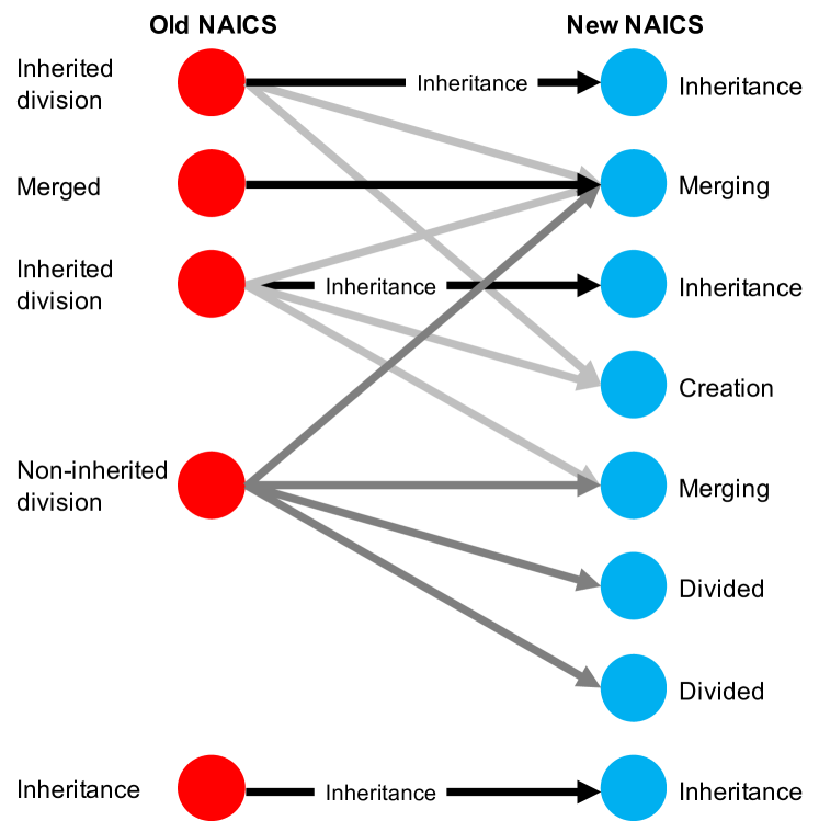
These temporal changes in industry classification define a bipartite network connecting old NAICS codes to new ones. For convenience, we refer to old codes as parents and we refer to new codes as children. All codes are classified into 7 groups: Inheritance (I), Creation (C), Merging (MG), Divided (D), Inherited Division (ID), Non-inherited Division (ND), and Merged (MD). This scheme exclusively and entirely classifies every code change in our dataset. The classification is defined by out-degrees of old codes and in-degrees of new codes in the connection structure.
Figure S2 shows the connection scheme for classification changes. Inheritance is the basic connection defined for simple one-to-one conversions of NAICS code. It is also defined for a code pair when the new code has , and the other new codes connected to the old code have . Briefly, only one new code exclusively inherits its parent as the old code is the only parent of the child. Inherited Division and Non-inherited Division are defined for old codes with (division), and depends on whether the old code has any inherited child or not. Creation, Merging and Divided are defined for new codes. A new code is determined as Creation when each of its parents has another inherited child. Merging is defined for the non-creation case that its parents has no other inherited child. A new node is considered as Divided when it has and is the child of a Non-inherited division node. Finally, Merged is defined for an old code that has and is the parent of a Merging code.
We translate all industry classifications to the most recent classification (2012) to make a harmonized time series of number of employees. In the case of inheritance (black arrows in Fig. S2), all employees in the old classification are transferred to the Inheritance node in the new classification. The division of employees colored by light grey is not transferred to the latter nodes, which means these connections are ignored. As a special case, Non-inherited division equally distribute its employment to the divided nodes (dark grey).
I.2 MSA revisions
Similar to the NAICS revisions, the Metropolitan Statistical Areas (MSAs) are revised about every 5 years. The exact time intervals are 1993-1999, 2000-2002, 2003-2006, 2007-2011 and 2012-2013. By using the conversion table obtained from American Association of State Highway and Transportation Officials (AASHTO), we harmonize all MSAs to a single reference. In 1998 and 1999, the MSAs are classified into two types: Consolidated Metropolitan Statistical Area (CMSA) and Primary Metropolitan Statistical Area (PMSA) where a CMSA contains several PMSAs. From 2000, MSAs have been revised to Combined Statistical Area (CBSA). For example, New York City is classified as ‘New York-Northern New Jersey-Long Island, NY-NJ-CT-PA’ CBSA, and ‘New York-Northern New Jersey-Long Island, NY-NJ-PA’ CMSA with 15 PMSAs including ‘Bergen-Passaic, NJ’, ‘Bridgeport, CT’, ‘Danbury, CT’, ‘Dutchess County, NY’, ‘Jersey City, NJ’, ‘Middlesex-Somerset-Hunterdon, NJ’, ‘Monmouth-Ocean, NJ’, ‘Nassau-Suffolk, NY’, ‘New Haven-Meriden, CT’, ‘New York, NY’, ‘Newark, NJ’, ‘Newburgh, NY-PA’, ‘Stamford-Norwalk, CT’, ‘Trenton, NJ’ and ‘Waterbury, CT’. For 1998 and 1999, we use CMSAs as the delineation of cities since CMSAs has a similar scale to CBSAs. When an MSA is divided into several MSAs or merged together with another MSA, we aggregated these MSAs to the largest one. Some exceptions are modified by using MSA definition provided by U.S. Census Bureau, and some megalopolises, such as New York, Los Angeles and Chicago, are cross-checked with the definitions in Wikipedia.
II Revealed comparative advantage
A
B
C
D
A
B
C
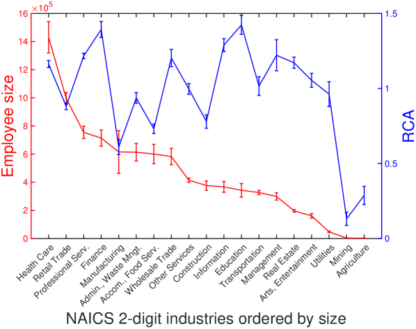
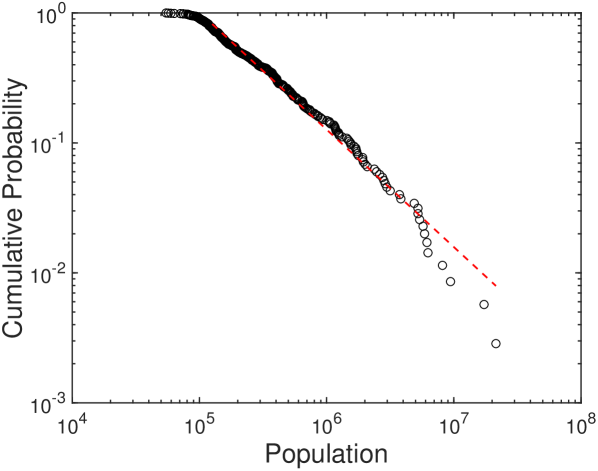
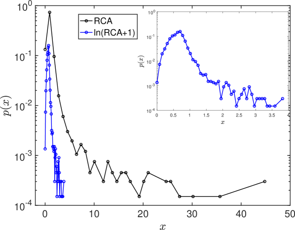
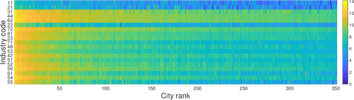
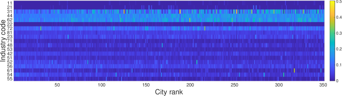
The raw size is the most representative indicator of employment or establishments. However, it has two limitations in capturing the characteristics of urban industry. First, the baseline industry sizes in cities make small industries indistinguishable. For example, the share of retail trade is 100 times larger than that of agriculture on average, and most cities have similar baseline industry composition as shown as the shares of industries in Figure S3B. A small industry can easily be shaded by a large industry with this considerable size differential. Furthermore, huge differences in city sizes can shade the characteristics of small cities. The power-law distribution of urban populations in Figure S4B demonstrates the high heterogeneity of city sizes. Figure S3A shows that large cities are dominating almost all industries when we see the unnormalized sizes. Therefore, the city sizes need to be normalized to compare the patterns in small and large cities.
Revealed Comparative Advantage (RCA) originated from international trade analysis Balassa (1965) and provides an ideal option for normalizing city sizes and industry sizes. RCA is defined as a ratio of urban share of an industry to the share of the industry across all cities. RCA can capture a small difference in industrial composition between cities by normalizing the urban industry size for both cities and industries. Figure S4A shows the industry size and its RCA for New York. The RCA normalizes tiny industries to comparable sizes.
In many studies Hidalgo et al. (2007); Hidalgo and Hausmann (2009), the presence of industry or production capability was considered as ”revealed” if its RCA is larger than 1. Since its presence and absence have asymmetric ranges in and , respectively, normalized RCA measures have been developed to make the range less heterogeneous. Logarithmic RCA () Vollrath (1991); Gao et al. (2017) is one of the normalized RCA measures.
| (S1) | ||||
| (S2) |
Compared to the logarithmic RCA, the original RCA has a highly heterogeneous distribution as in Fig. S4C. An urban industry with extraordinarily high or low RCA value makes other general industries very insignificant.
III Urban scaling relation
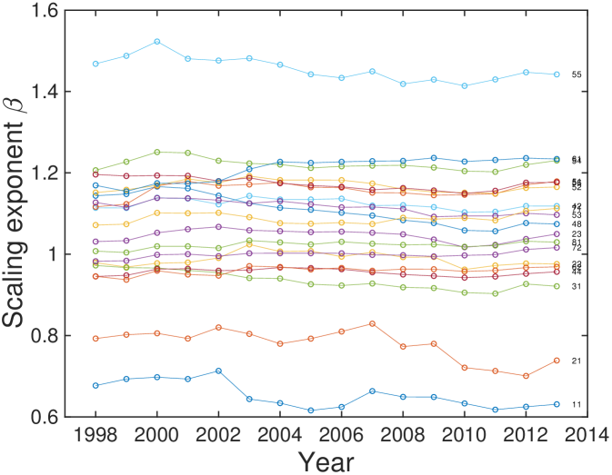
Previous work has shown the scaling relationship of urban employment by industry Youn et al. (2016). Accordingly, we calculate the scaling exponents and the pre-factors of industries for the size of employment and the city size by fitting the following equation to empirical employment data:
| (S4) |
The industry size has high fluctuations in the low level of classifications. Therefore, we use 2-digit NAICS resolution. We calculate the scaling exponent by taking linear regression on the logarithms of and for a fixed industry and a time . The time-average of scaling exponents in 1998 to 2013 and the corresponding temporal deviation are listed in Table. S1. Scaling exponents do not show much temporal change during the time period of this study (see Fig. S5).
| Industry | NAICS code | ||
| Agriculture, Forestry, Fishing and Hunting | 11 | 0.65 0.03 | 0.31 0.04 |
| Mining, Quarrying, and Oil and Gas Extraction | 21 | 0.78 0.04 | 0.31 0.04 |
| Manufacturing | 31 | 0.94 0.02 | 0.73 0.02 |
| Retail Trade | 44 | 0.96 0.01 | 0.98 0.00 |
| Health Care and Social Assistance | 62 | 0.96 0.01 | 0.94 0.00 |
| Utilities | 22 | 0.99 0.02 | 0.66 0.02 |
| Accommodation and Food Services | 72 | 1.00 0.01 | 0.95 0.00 |
| Other Services (except Public Administration) | 81 | 1.02 0.01 | 0.95 0.00 |
| Construction | 23 | 1.05 0.01 | 0.92 0.01 |
| Arts, Entertainment, and Recreation | 71 | 1.09 0.01 | 0.86 0.01 |
| Transportation and Warehousing | 48 | 1.11 0.04 | 0.85 0.01 |
| Real Estate and Rental and Leasing | 53 | 1.12 0.02 | 0.93 0.00 |
| Wholesale Trade | 42 | 1.12 0.01 | 0.91 0.01 |
| Information | 51 | 1.16 0.02 | 0.89 0.01 |
| Finance and Insurance | 52 | 1.17 0.01 | 0.88 0.01 |
| Administrative and Support and Waste Management and Remediation Services | 56 | 1.17 0.02 | 0.93 0.01 |
| Educational Services | 61 | 1.21 0.03 | 0.77 0.01 |
| Professional, Scientific, and Technical Services | 54 | 1.22 0.01 | 0.92 0.01 |
| Management of Companies and Enterprises | 55 | 1.46 0.03 | 0.76 0.02 |
IV Lead-follow matrix
IV.1 Definition of lead-follow matrix
We normalize the size of urban employment using RCA in Eq. S2. By using the RCA values, we characterize the industries in a city as industry vector of city in year . The spatial vector of industry can be defined in a similar way.
| (S5) | ||||
| (S6) |
where , and denote the logarithmic RCA, the set of industries, and the set of cities, respectively. The length of the industry vector is equal to the number of industries (e.g. 19 for 2-digit NAICS industries). The industrial similarity between two cities and with a time lag is now measured by a Pearson correlation between two vectors and .
| (S7) |
where measures the Pearson correlation between two vectors. The inter-industry locational similarity can also be obtained for the location vector .
As the dynamics of each city fluctuates, we group the cities by their populations, and use the average population as the reference.
| (S8) |
where denotes the average for the cities in group . We usually group the cities into 20 groups of equal sizes. The industrial similarity between groups can also be defined using their correlations as in Eq. S7.
| (S9) |
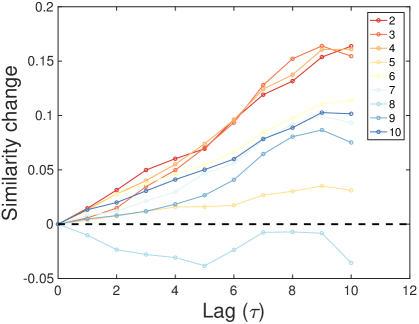
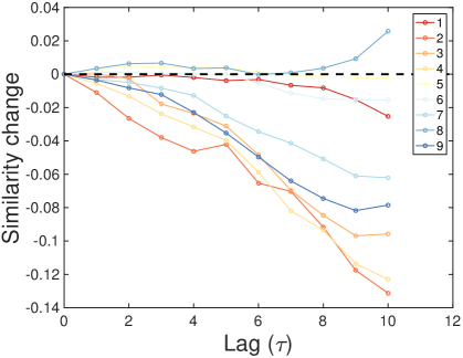
Then, we fix one group as a reference group, let another group evolve in time (), and measure their industrial similarity . By following the change of industry similarity as time lag changes, we can observe if group is getting similar or dissimilar to group in time. To focus on the effect by time lag , we average the change over the reference times .
| (S10) | ||||
| (S11) |
where is the average change of similarity between reference group and observed group for time difference . Figure S6A and Figure S6B show the trends of versus on lag for a fixed reference group and various observed group denoted by colored lines. In Fig. S6A, the similarity generally increases for the largest reference city, which means that small cities get similar to the largest cities in time. On the other hand, large cities get dissimilar to the smallest group in Fig. S6B. These trends show the directional evolution of urban economy led by large cities and followed by small cities. We summarize these trend in the form of matrix.
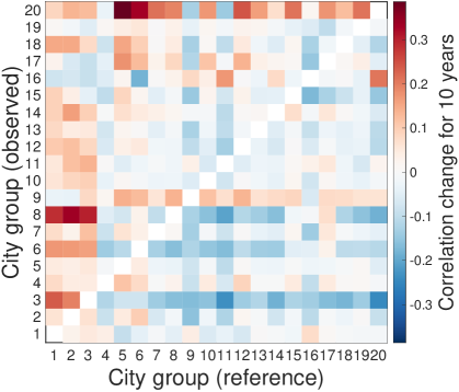
Finally, we measure the average similarity change between groups for years, which is called “Lead-follow matrix” denoted as . We set as 10 years considering the time span of our data. The average rate is obtained by the least squares method.
| (S12) | ||||
| (S13) |
Figure S6C summarizes the time-lag similarities across cities as a “Lead-Follow Matrix”. The general pattern observed in the figures is that small cities get similar to larger cities whereas large cities get dissimilar from smaller cities. As the city groups are ordered by their population sizes, the upper triangle represents the temporal behavior of small cities on the larger cities on x-axis, whereas the lower triangle describes the behavior of larger cities. The positive values in the upper triangle mean that small cities become more and more similar to the past of large cities, recapitulating, in terms of their industrial characteristics, while the negative values in the lower triangle represent that large cities grow away from the past of smaller cites as time goes. The asymmetric shape indicates that the evolution of urban industry has a clear direction that large cities lead the change and small cities follow the path from behind. In other words, the largest 3 city groups (top 60 cities) are considered as main leaders from their significant patterns in the lead-follow matrix.
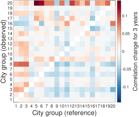
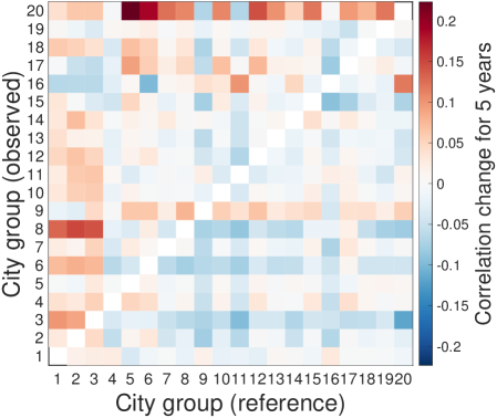
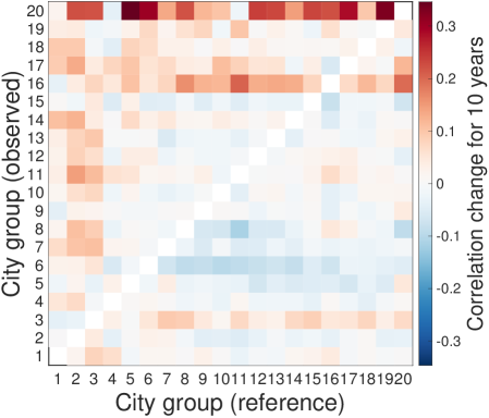
IV.2 Robustness check
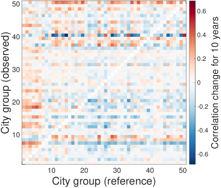
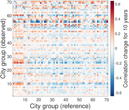
We check the robustness of the lead-follow matrix for various conditions: length of time lags, NAICS level, and number of city groups. We test the time lags for 3 and 5 years, NAICS for 3- and 4-digits, and city groups for 50 groups and 70 groups based on the the reference parameters for 10-years time lags, 2-digit NAICS, and 20 city groups. As a result, the lead-follow matrix is robust for the variants of time lags, NAICS digits, and city group sizes.
A B C
A
B
C
D
E
F
V Integrated framework
V.1 Time-independent integrated framework of RCA and scaling relation

By the scaling relation, the size of industry in a city with population size is given as follows:
| (S14) |
The pre-factor and the scaling exponent are obtained by taking a regression on and for each industry . By definition, the revealed comparative advantage (RCA) can be expressed as a function of population and scaling exponent.
| (S15) |
where is a constant. Since is the total size of industries in a city, it can be approximated to be proportional with . The total industry size for all cities, , is estimated by continuous population approximation, whose distribution follows . For , the summation becomes,
| (S16) |
For , the summation can be determined by either taking limitation or changing the integration to .
| (S17) |
where and by definition. The same result can be achieved by changing the integration as,
| (S18) |
As a result, the RCA is approximated as,
The scaling exponent of population distribution generally equals to 2 for cities following the Zipf’s law. For , the RCA is approximated as,
| (S19) |
The derived RCA has different trends by population sizes. Approximately, RCA is proportional to for large while it is inversely proportional to for small . In that case, if we correlate the RCA vectors of small and large cities, the correlation becomes negative while the correlations inside small cities and large cities remain positive. This property generates two clusters of small and large cities.
V.2 Fixed point of city clustering
Now, we find the characteristic city size that distinguishes the small and large cities. The characteristic size is given as a saddle point of Eq. S19. The saddle point should satisfy both and . Since is continuous, we only consider the case for in the calculation of the saddle point.
Therefore, . The above conditions mean that the saddle point exists only if the probability of scaling exponent around is not zero. For example, if every scaling exponent is larger than 1 or smaller than 1, the saddle point needed for clustering of cities does not exist.
where and . Therefore, the saddle point population is given at,
| (S20) | ||||
| (S21) |
where . The saddle-point population is calculated as 1.2 millions for , and , which is similar with the observation in data.
As a result of connection between RCA and scaling relations, we can expect the clustering of cities by their industrial compositions. Fig. S8A is the result obtained by the Pearson correlations between industry vectors of cities characterized by RCA with 2-digit industry classifications. The clustering of cities is clearly observed with a fixed point near 50th largest city.
We can also figure out the fixed point using the trends in Fig. S8B. RCA as a function of and in Eq. S19 can be simplified by taking logarithm on both sides.
| (S22) |
.
Logarithm of RCA becomes a linear function of with a slope . It makes the trend inverted when changes from to , and generates two clusters by their populations.
V.3 Time-dependent integrated framework of RCA and scaling relation
To understand the time-dependent behavior of RCA following the scaling relation, we derive the time-dependent equation of RCA under several assumptions. In addition to two assumptions (i.e., (1) power-law distributed population, (2) total employee size in a city) used in the time-independent derivation, we include two additional assumptions: (3) total national employee size proportional to the summation of the total populations, and (4) time-independent , , , and . The third assumption is given from the second assumption by definition.
| (S23) |
where the second assumption is given as for time-dependent constant . For the fourth assumption, the scaling exponent and the pre-factor do not change much in time as in Fig. S5, and the scaling exponent of the population distribution is also not expected to change much in time. For the maximum and minimum populations, the average urban population change between the first year (1998) and the last year (2013) is about 23%, so we can marginally assume its time-independency when we observe the dynamics in a short period. Four assumptions are listed as follows:
-
1.
-
2.
-
3.
-
4.
Time-independent , , , and .
We can derive the time-dependent RCA by substituting the time-dependent industry size in the definition.
| (S24) | ||||
| (S25) | ||||
| (S26) |
The summations can be obtained using the approximation of power-law distributed continuous populations (assumption 1).
| (S27) |
| (S28) |
Finally, we can obtain the closed-form time-dependent RCA as a function of , , and .
| (S29) | ||||
| (S30) |
where is a time-invariant constant for simplifying the equation. Since the only time-variant term is , the time-derivative of RCA depends only on the time-derivative of population. For easy calculation, we take logarithm on both sides and take the derivatives.
| (S31) | ||||
| (S32) |
One interesting thing of these equations is the analogy with the scaling relation of size. Following the scaling relation , the log size and its time-derivative have similar forms with RCA except the difference in the proportional constant, 1.
| (S33) | ||||
| (S34) |
In that sense, RCA is similar to a coordinate transformation that makes a projection of scaling relation onto -axis, because a scaling relation usually have a slope close to 1. One remarkable advantage of using RCA is its sensitivity to super- or sub-linearity. For the situation that the urban scaling relation is valid, the size of every industry always grows if its urban population grows, however, the RCA depends on whether each industry has superlinear or sublinear scaling.
-
1.
For and , .
-
2.
For and , .
-
3.
For and , .
-
4.
For and , .
The dependency of RCA on populations can be a more intuitive measure of superlinearity or sublinearity of the industry, i.e., a superlinear scaling for positive correlation and a sublinear scaling for negative correlation.
V.4 Diversity by the number of characteristic industries
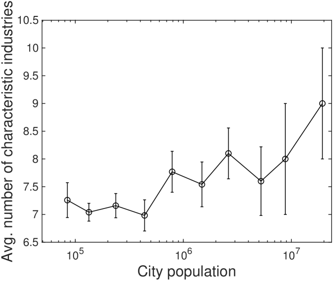
Fig. S8B and Eq. S31 show that industries with is characteristic in small cities, and industries with is characteristic in large cities. becomes the reference of small cities and large cities. We can expect that the distribution of will determine the number of characteristic industries by city size. There are fewer industries with than industries with , therefore, the number of characteristic industries is expected to increase with city size.
Fig. S9 shows that this expectation is true in our urban employment data. Small cities with have fewer characteristic industries, about 7 industries out of 19 industries, while large cities have more characteristic industries, about 8-9 industries. It shows the increase of industrial diversity as city size increases.
VI Urban recapitulation
VI.1 Trajectory of cities for each industry
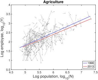
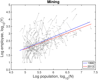
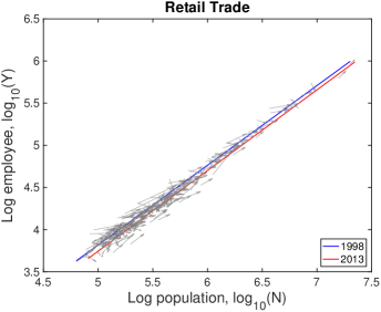
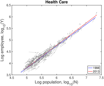
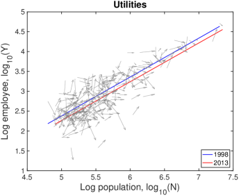
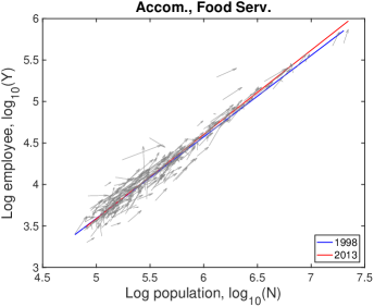
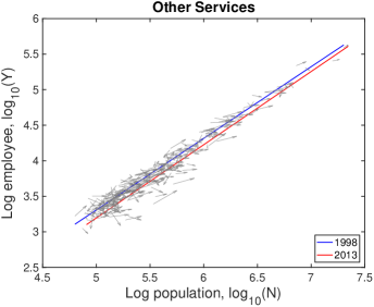
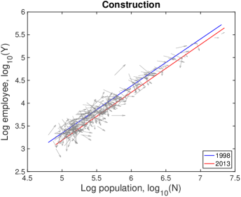
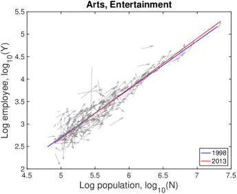
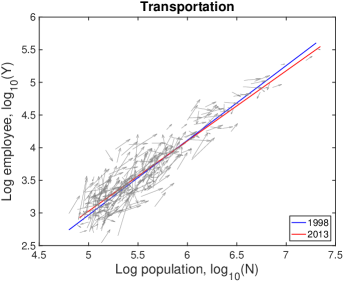
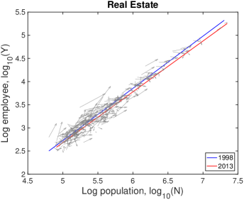
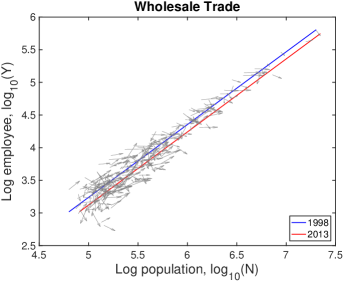
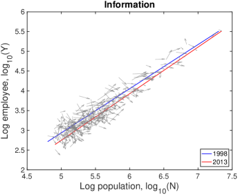
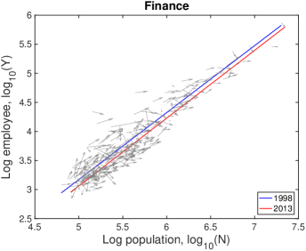
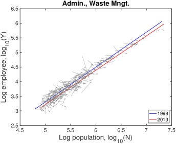
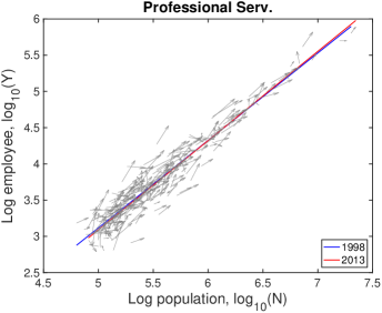
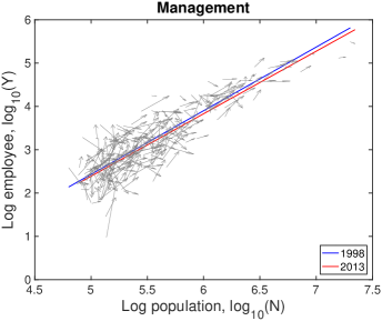
The growth of population and industry size of cities can be represented as trajectories in the population-industry plane like the scaling relation. We present the trajectory of each city as arrows for 2-digit NAICS industries in Fig. S10. In some industries, most of cities grow following the fitting line of scaling relation, but they drift or irregularly move in some industries. The scaling relation for the cross-sectional view gives an insight on explaining the dynamics. We linearize and differentiate the time-dependent scaling relation to mathematically formulate the dynamics. Since the scaling exponent does not change much in our time scope (Fig. S5), we can consider the scaling exponent as constant in time (i.e., denoted as ).
| (S35) | ||||
| (S36) | ||||
| (S37) |
where means the difference of a value of between the start year (1998) and the end year (2013) of our time scope, i.e., . Eq. S37 decomposes the growth into time-dependent global growth and population-dependent growth . The trajectories in Fig. S10 directly present these decomposition of growth that the global shift is based on and the city-specific local movement is based on .
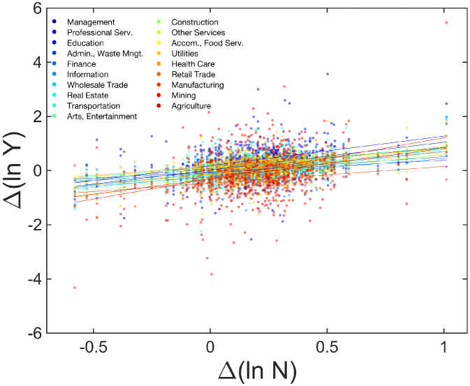
Based on Eq. S37, we measure the change of industry size versus on the change of population of each city. Fig. S11A shows common positive correlations between them. By Eq. S37, the slope of each industry, longitudinal size-dependency, should be the same with the cross-sectional scaling exponent . We obtain the longitudinal size-dependency by taking a linear regression on the scatter plot in Fig. S11A. The comparison of the slope and the scaling exponent is depicted in Figure S11B. If the dynamics perfectly follows the theoretical expectation by scaling relations, all data points should be on the prediction line (red dot). Although they are not perfectly matched, the scaling relation predicts its general trend, that is, the direction of industry size change is coherent with the direction of population change.
VI.2 Recapitulation scores
The degree of recapitulation can be measured from how much each city follows the fitting line. Let us consider the case of perfect recapitulation. In that case, the trajectory of every city will lie exactly on the fitting line. When a city population grows, its industry size should accordingly grow following the fitting line. In that case, the measured growth terms , and using Eq. S37 and Fig. S11A quantify how much the real data follows the dynamics predicted by theory. Since the amount of drift only shifts the fitting line, we can measure the “degree of recapitulation” by comparing longitudinal size-dependency and cross-sectional scaling exponent . The difference between them becomes a direct measure of recapitulation of each industry. We define the recapitulation score of each industry using the relative error of to average in our time scope.
| (S38) |
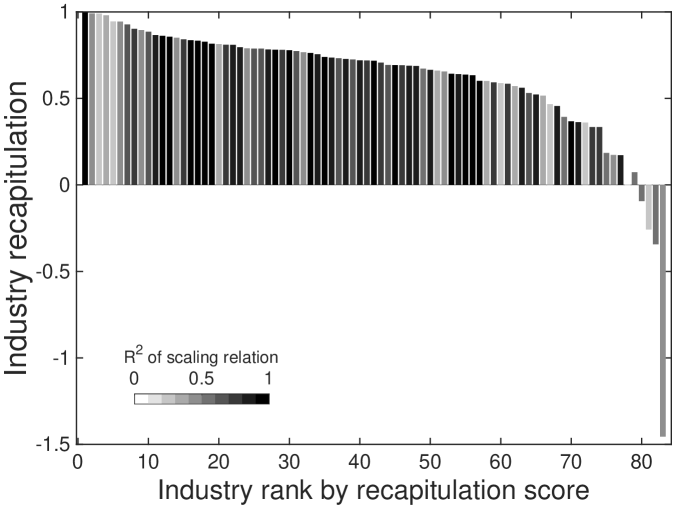
The score becomes maximum () when , and it becomes zero when has no tendency (. When has the opposite sign of , the score becomes negative. The recapitulation scores for 2-digit and 3-digit industries are shown in Fig. S11C and Fig. S11D. The average recapitulation score of industries with significant scaling relation () is 0.70 which validates the existence of recapitulation in cities. The significantly low scores of ‘Agriculture’ and ‘Mining’ industries seem to originate from their strong dependency on regional characteristics.
Now, how can we measure the degree of recapitulation in each city? For that, we need to define a measure of industrial growth of individual city in the scaling framework. Using the measured global growth in Eq. S37, we can estimate the coefficient of growth of a city for a specific industry . As the equation was defined for an industry, it can easily be generalized using an industry index .
| (S39) | ||||
| (S40) |
The coefficient denotes the ratio of industry growth to the population growth in city . Since many cities have a small relative population change as depicted in Fig. S11A, in a city scale is very fluctuating. To observe a general trend, we group the cities into 20 groups and measure the averaged slope of versus on using least square errors.
| (S41) |
The measured is the coefficient of population-dependent growth of city group for industry . It should be the same with when every city in perfectly recapitulates. The city group recapitulation score of group for industry can be measured in the same way of Eq. S38.
| (S42) |
Finally, the city group recapitulation score for every urban industry can be defined as the average of recapitulation scores for each industry .
| (S43) | ||||
| (S44) |
where is the number of industries.
VI.3 Detailed explanation on the drifts
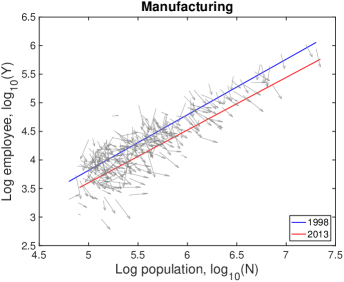
In Fig. S10, each city moves on the population-industry size space as time proceeds, and their trend can be described by the scaling relation. In many cases such as “Manufacturing”, the fitting line in 2013 is at the bottom-right side of the fitting line in 1998 with little change of slope. Does it mean decrease in industry size contradicting to the overall increase in Fig. S1B? It depends on the ratio of relative industry growth to relative population growth, and it does not contradict to the overall increase. Let us see the details with mathematical formulation.
As a fitting line is obtained for the scaling relation in the log-log scale, this shift of the fitting line can be caused by a uniform relative change of populations or industry sizes. Let these relative changes of populations and industry sizes be and for city and industry . For convention, let us consider only the change between the initial year, 1998, and the last year, 2013, in our scope.
| (S45) | ||||
| (S46) |
Since the difference of logarithmic values is equivalent to the relative change, , the fitting line of scaling relation may shift in the horizontal direction when every city undergoes a uniform relative population growth, . In the same way, the fitting line moves in the vertical direction when every city undergoes a uniform relative industry growth, . The fitting line moves to a lower side when the population growth is not followed by a sufficient industry growth. To stay in the current position, the fitting line should move vertically in when it moves horizontally in . We can also derive it from the time derivative of scaling relation in Eq. S37.
| (S47) | |||
| (S48) |
Therefore, the red lines under the blue lines in Fig. S10 do not mean the actual decrease in the industry size. It is caused by a relatively lower industry growth than the population growth, i.e., . Similarly, the fitting line moving upward as in ‘Health Care’ industry is given by a relatively higher industry growth with .
VI.4 Time-dependent scaling relation from industry size and population changes
Now, let us consider that the relative changes of populations and industries are not uniform across cities. It can be described as a function of and for city . Fig. S11A shows their relations for NAICS 2-digit industries. It can be simplified to a linear relation,
| (S49) |
where is a global growth across all cities, and is the coefficient of population-dependent growth. Using , we can derive the time-dependent scaling relation.
| (S50) | ||||
| (S51) |
where . Since the scaling relation is given as , the equation can be expressed as a perturbed form.
| (S52) |
| (S53) |
where and . Since is the second order term, we can obtain an approximated scaling relation for in the case of small difference between and .
| (S54) |
where means a global exponential growth. From the above derivation, the global growth term is related to the growth of . It represents a global drift of every city in industry space. The population-dependence coefficient is related to the scaling exponent . When there is little difference between and as in our data, the scaling exponent at the later time becomes the same with .
A
B
C
D
E
F
| Industry | NAICS code | |||
| Agriculture, Forestry, Fishing and Hunting | 11 | 0.65 | 1.13 | -0.31 |
| Mining, Quarrying, and Oil and Gas Extraction | 21 | 0.78 | 1.51 | -0.30 |
| Manufacturing | 31 | 0.94 | 0.62 | -0.47 |
| Retail Trade | 44 | 0.96 | 0.82 | -0.12 |
| Health Care and Social Assistance | 62 | 0.96 | 0.66 | 0.15 |
| Utilities | 22 | 0.99 | 1.20 | -0.30 |
| Accommodation and Food Services | 72 | 1.00 | 0.69 | 0.10 |
| Other Services (except Public Administration) | 81 | 1.02 | 0.76 | -0.15 |
| Construction | 23 | 1.05 | 0.86 | -0.28 |
| Arts, Entertainment, and Recreation | 71 | 1.09 | 0.77 | 0.66 |
| Transportation and Warehousing | 48 | 1.11 | 0.72 | 0.14 |
| Real Estate and Rental and Leasing | 53 | 1.12 | 0.85 | -0.09 |
| Wholesale Trade | 42 | 1.12 | 0.88 | -0.18 |
| Information | 51 | 1.16 | 0.67 | -0.23 |
| Finance and Insurance | 52 | 1.17 | 0.59 | -0.07 |
| Administrative and Support and Waste Management and Remediation Services | 56 | 1.17 | 0.44 | -0.06 |
| Educational Services | 61 | 1.21 | 1.09 | 0.18 |
| Professional, Scientific, and Technical Services | 54 | 1.22 | 0.78 | 0.07 |
| Management of Companies and Enterprises | 55 | 1.46 | 1.03 | 0.02 |