A Comparative Analysis of Scale-invariant Phenomena in Repeating Fast Radio Bursts and Glitching Pulsars
Abstract
The recent discoveries of a remarkable glitch/antiglitch accompanied by fast radio burst (FRB)-like bursts from the Galactic magnetar SGR J1935+2154 have revealed the physical connection between the two. In this work, we study the statistical properties of radio bursts from the hyperactive repeating source FRB 20201124A and of glitches from the pulsar PSR B1737–30. For FRB 20201124A, we confirm that the probability density functions of fluctuations of energy, peak flux, duration, and waiting time well follow the Tsallis -Gaussian distribution. The derived values from -Gaussian distribution keep approximately steady for different temporal interval scales, which indicate that there is a common scale-invariant structure in repeating FRBs. Similar scale-invariant property can be found in PSR B1737–30’s glitches, implying an underlying association between the origins of repeating FRBs and pulsar glitches. These statistical features can be well understood within the same physical framework of self-organized criticality systems.
1 Introduction
Fast radio bursts (FRBs) are intense millisecond-duration astronomical transients with mysterious physical origins (Lorimer et al., 2007; Xiao et al., 2021; Petroff et al., 2022; Zhang, 2023). Some FRB sources, such as FRB 20121102 (Spitler et al., 2016) and FRB 20201124A (Lanman et al., 2022), have been seen to burst repeatedly, but it is still unclear whether repeating FRBs are prevalent or rare sources. Nonetheless, the statistical analysis of the repetition pattern may shed new light on the physical nature and emission mechanisms of FRBs (e.g., CHIME/FRB Collaboration et al. 2020a; Rajwade et al. 2020; Zhang 2020; Cruces et al. 2021; Li et al. 2021b).
By studying the statistical properties of the repeating bursts from FRB 20121102, Lin & Sang (2020) and Wei et al. (2021) found that the probability density functions (PDFs) of fluctuations of energy, peak flux, and duration well follow a -Gaussian distribution. Here the fluctuations are defined as the size (energy, peak flux, or duration) differences at different times. Furthermore, such a -Gaussian behavior does not depend on the time interval adopted for the fluctuation, i.e., the values in -Gaussian distributions are approximately equal for different temporal interval scales, which implies that there is a scale-invariant structure in FRB 20121102 (Lin & Sang, 2020; Wei et al., 2021). Analogous scale-invariant characteristics have also been found in earthquakes (Caruso et al., 2007; Wang et al., 2015), soft gamma-ray repeaters (SGRs; Chang et al. 2017; Wei et al. 2021; Sang & Lin 2022), X-ray flares (Wei, 2023) and precursors (Li & Yang, 2023) of gamma-ray bursts (GRBs), and gamma-ray flares of the Sun and the blazar 3C 454.3 (Peng et al., 2023). It is suggested that scale invariance is the most essential hallmark of a self-organized criticality (SOC) system (Caruso et al., 2007; Wang et al., 2015). A generalized definition of SOC is that a nonlinear dissipative system with external drives input will self-organize to a critical state, at which a small local disturbance would generate an avalanche-like chain reaction of any size within the system (Bak et al., 1987). Since the concept of SOC was proposed (Katz, 1986; Bak et al., 1987), it has been extensively used to explain the dynamical behaviors of astrophysical phenomena (Aschwanden, 2011, 2012, 2014, 2015; Aschwanden et al., 2016).
On 2020 April 28, a bright radio burst FRB 20200428 was independently detected by CHIME (CHIME/FRB Collaboration et al., 2020b) and STARE2 (Bochenek et al., 2020) in association with a hard X-ray burst from a Galactic magnetar named SGR J1935+2154 (Mereghetti et al., 2020; Li et al., 2021a; Ridnaia et al., 2021; Tavani et al., 2021). This discovery provided the first evidence for the magnetar origin of at least some FRBs (Zhang, 2020). Since this event, NICER and XMM-Newton telescopes have been monitoring SGR J1935+2154 regularly in the 1–3 keV band. A phase-coherent timing analysis of X-ray pulses from the source was employed and a large spin-down glitch (also referred to as “antiglitch”) with Hz was detected on 2020 October 5 ( day) (Younes et al., 2023). Subsequently, three FRB-like radio bursts emitted from SGR J1935+2154 were detected by the CHIME/FRB system on 2020 October 8 (Good & Chime/Frb Collaboration, 2020). More surprisingly, Ge et al. (2022) utilized the observations from NICER, NuSTAR, Chandra, and XMM-Newton to study the timing properties of SGR J1935+2154 around the epoch of FRB 20200428, and reported that a giant spin-up glitch with Hz occurred approximately day before FRB 20200428.
Glitches have now been observed in over a hundred pulsars, which are characterized as sudden increases in the rotational frequency of the star. Despite several decades of research, the physical mechanisms of glitches are still not completely understood, but probably involve an interaction between the neutron star’s outer elastic crust and the superfluid component that lies within (see Haskell & Melatos 2015; Antonopoulou et al. 2022 for reviews). The spin-down events, known as antiglitches, are even rarer than glitches, and lack of observational data. The exact origin of antiglitches is also still open to debate (Thompson et al., 2000; Huang & Geng, 2014; Mastrano et al., 2015). The temporal coincidences between the glitch/antiglitch and FRB-like bursts of SGR J1935+2154 reveal the physical connection between the two (Ge et al., 2022; Wu et al., 2023; Younes et al., 2023). Motivated by this, we here examine the scale-invariant similarities between repeating FRBs and glitching pulsars.
Since the sample size of most repeaters in the past was small, FRB 20121102 with relatively more repeating bursts is so far the only source that has been used to study the scale-invariant property (Lin & Sang, 2020; Wei et al., 2021). As more hyperactive repeaters have been detected, it is interesting to find out whether other FRBs share the same scale-invariant property. One of the most hyperactive repeating sources to date is FRB 20201124A, with 2744 independent bursts detected by the Five-hundred-meter Aperture Spherical radio Telescope (FAST), representing the largest sample for a single observation (Xu et al., 2022; Zhang et al., 2022). In addition, Kirsten et al. (2024) reported the detection of 46 high-energy bursts111Note that in this paper, “high-energy burst” refers to bursts with large values of their isotropic energies, rather than bursts detected at higher observing frequencies. from FRB 20201124A in more than 2000 hours using four small 25–32-m class radio telescopes. The energy distribution slope of these high-energy bursts is much flatter than that of the high-energy tail in the FAST data, suggesting that ultra-high-energy ( erg) bursts occur at a much higher rate than expected based on FAST observations of lower-energy bursts (Kirsten et al., 2024). The study on the scale-invariant properties of low- and high-energy bursts would be helpful for judging whether the highest-energy bursts originate from a different emission mechanism or emission region at the progenitor source. On the other hand, for glitching pulsars, their scale-invariant property has not yet been explored. However, because glitches are infrequent events, the number of detected glitches in most of pulsars is not substantial enough to carry out robust statistical analyses on individual bases (Fuentes et al., 2019). To date, 37 glitches in PSR B1737–30 have been detected, and these glitches exhibit a power-law size distribution. It should be underlined that the SOC systems would be slowly driven toward a critical state of the instability threshold of the entire system, leading to scale-free power-law size distributions (Aschwanden, 2014). Thus, the emergence of a power-law size distribution is another fundamental property that SOC systems have in common (Aschwanden, 2011, 2012, 2015), suggesting that PSR B1737–30 has enough glitches for studying its scale-invariant feature.
In this work, we investigate and examine the similar scale-invariant phenomena between FRB 20201124A and glitches of PSR B1737–30. Moreover, in view of the fact that the burst energy distribution of FRB 20201124A flattens towards the highest-observed energies, the sensitivity limits of FAST and 25–32-m class radio telescopes are different, and the statistical characteristics of 46 high-energy bursts would be submerged in the large amount of FAST data for the combined analysis, the scale-invariant behaviors of low- and high-energy bursts from FRB 20201124A are thus studied separately. The rest parts of this article are organized as follows. In Section 2, we make the scale-invariant analyses on energy, peak flux (luminosity), duration, and waiting time of low- and high-energy bursts from FRB 20201124A, respectively. In Section 3, taking PSR B1737–30 as an example, the distributions of fluctuations of glitch size and of waiting time between consecutive glitches are presented for the first time. Finally, relevant conclusions are drawn in Section 4.
2 Scale Invariance in FRB 20201124A
2.1 Statistical properties of the FAST data
Recently, Xu et al. (2022) and Zhang et al. (2022) reported in total 2744 bursts from the repeating source FRB 20201124A detected by FAST from April 1 to June 11 and September 25 to October 17 in 2021. These observations were performed in the frequency range 1.0–1.5 GHz by using the center beam of the 19-beam receiver. Xu et al. (2022) detected 1863 bursts in 82 hours over 54 days, and Zhang et al. (2022) detected 881 bursts in 4 hours over 4 days. All these data were recorded with a frequency resolution of 122.07 kHz (i.e., using 4096 frequency channels to cover 1.0–1.5 GHz) and a time resolution of 49.152 s (Xu et al., 2022; Zhang et al., 2022; Zhou et al., 2022). The total of 2744 bursts from FRB 20201124A is at present the largest sample observed with a single instrument and uniform selection effects. In this work, we use this sample to study the PDFs of fluctuations of energy, peak flux, duration, and waiting time. FRB 20201124A was localized in a massive star-forming galaxy with a spectroscopic redshift of (Fong et al., 2021; Piro et al., 2021; Ravi et al., 2022; Xu et al., 2022). The known redshift allows us to infer the isotropic energy of each burst through , where is the luminosity distance, is the burst fluence, and is the bandwidth. The waiting time is evaluated by the difference of times-of-arrival of two adjacent bursts.
The fluctuation of a size (e.g., energy, peak flux, duration, or waiting time) is defined as
| (1) |
where is the size of the -th burst (or of the -th pulsar glitch, more on this below) in temporal order, and is an arbitrary integer denoting the temporal interval scale. In order to simplify the calculation, is rescaled by
| (2) |
where is the standard deviation of . We will analyze the statistical properties of the dimensionless fluctuations .
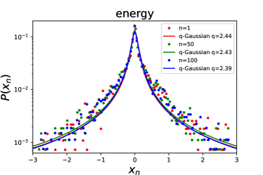
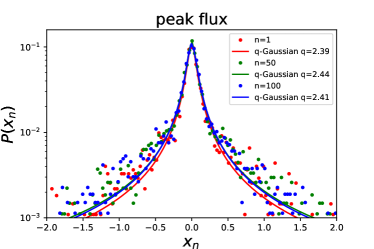
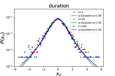
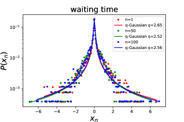
Figure 1 shows the statistical results of FRB 20201124A for the FAST sample. We plot as colour dots the PDFs of fluctuations of energy (upper-left panel), peak flux (upper-right panel), duration (lower-left panel), and waiting time (lower-right panel) for the temporal interval scale (red dots), (green dots), and (blue dots). Empirically, the data are binned with the Freedman-Diaconis rule (Freedman & Diaconis, 1981). One can see from Figure 1 that compared to a Gaussian distribution, these PDFs have a sharper peak at and fatter tails. The sharp peak indicates that small fluctuations are most likely to occur, while fat tails indicate that there are large but rare fluctuations. Another remarkable feature is that the data points in Figure 1 are almost independent of the interval considered for the fluctuation, suggesting a common behavior of . Here we use the Tsallis -Gaussian function (Tsallis, 1988; Tsallis et al., 1998)
| (3) |
to fit , where is a normalization factor, the parameters and determine the sharpness and width of the distribution, respectively. The -Gaussian function is a generalization of the standard Gaussian function, and it reduces to a Gaussian shape with zero mean and standard deviation when gets close to 1. Thus, means a departure from Gaussian behavior.
| FRB 20201124A | |||
|---|---|---|---|
| for the FAST sample | |||
| parameters | |||
| -energy | |||
| 1.68 | 1.35 | 1.47 | |
| -peak flux | |||
| 0.94 | 0.89 | 0.89 | |
| -duration | |||
| 0.87 | 0.77 | 1.04 | |
| -waiting time | |||
| 1.60 | 2.03 | 1.57 | |
| FRB 20201124A | |||
| for the high-energy burst sample | |||
| parameters | |||
| -energy | |||
| 0.05 | 0.13 | 0.13 | |
| -luminosity | |||
| 0.11 | 0.05 | 0.08 | |
| -duration | |||
| 0.09 | 0.09 | 0.15 | |
| -waiting time | |||
| 0.18 | 0.11 | 0.13 | |
| PSR B1737–30 | |||
| parameters | |||
| -glitch size | |||
| 0.40 | 0.37 | 0.51 | |
| -waiting time | |||
| 0.13 | 0.09 | 0.41 | |
| FRB name | Instrument | Energy range | Number | -energy | -flux | -duration | -waiting time | Refs. |
| (erg) | ||||||||
| 20121102 | FAST | – | 1652 | – | 1 | |||
| 20201124A | FAST | – | 2744 | 2 | ||||
| 20201124A | St, O8, Tr, Wb | – | 46 | 2 | ||||
| PSR name | Observatory | Glitch size range | Number | -glitch size | -waiting time | Refs. | ||
| (Hz) | ||||||||
| B1737–30 | JBO | – | 37 | 2 |
For a specific , the free parameters (, , and ) can be optimized by minimizing the statistics,
| (4) |
where is the uncertainty of the data point, with being the number of in the -th bin and being the total number of (Wei et al., 2021). Note that for the sake of clarity, the error bars of the data points are not plotted in the figure. We then adopt the Python Markov Chain Monte Carlo module, EMCEE (Foreman-Mackey et al., 2013), to perform the fitting. The red, green, and blue curves in Figure 1 stand for the best-fitting results for , , and , respectively. The best-fitting values and their uncertainties for are listed in Table 1, along with the reduced value for the fit. It is obvious that the PDFs of fluctuations of energy, peak flux, duration, and waiting time are well reproduced by means of -Gaussians.
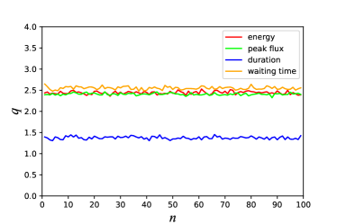
With the FAST data, we further extract the PDFs of fluctuations of energy, peak flux, duration, and waiting time for different scale intervals , and fit the PDFs with the -Gaussian function. The best-fitting values as a function of for energy, peak flux, duration, and waiting time are displayed in the left panel of Figure 2. One can see that the values are approximately invariant and do not depend on the scale interval , implying a scale-invariant structure of FRB 20201124A. The mean values of for energy, peak flux, duration, and waiting time of the FAST data are , , , and , respectively, which are listed in Table 2. Here the uncertainties represent the standard deviations of values. Interestingly, the values we derived here are very close those of FRB 20121102 (Wei et al., 2021), which suggest that there is a common scale-invariant structure in repeating FRBs.
Xu et al. (2022) estimated the sample completeness for the FAST data, and showed that the fluence threshold achieving the 95% detection probability with a signal-to-noise ratio is 53 mJy ms. To investigate how the completeness threshold would affect the modelling by -Gaussians, we also perform a parallel comparative analysis of the complete subsample (i.e, those bursts with mJy ms). We find that the mean values of for energy, peak flux, duration, and waiting time are , , , and , respectively. Comparing these inferred values with those obtained from the whole FAST sample (see line 2 in Table 2), it is clear that the completeness threshold in the energy distribution only has a minimal influence on our results.
2.2 Statistical properties of high-energy bursts
Using four small 25–32-m class radio telescopes (including the 25-m telescope in Stockert, Germany (St); the 25-m dish in Onsala, Sweden (O8); the 32-m dish in Toruń, Poland (Tr); and the 25-m dish in Westerbork, The Netherlands (Wb)), Kirsten et al. (2024) detected 46 high-energy bursts from FRB 20201124A. They concluded that the highest-energy bursts ( erg) occur much more frequently than one would expect based on the energy distribution of lower-energy bursts observed by FAST. The hyperactive source FRB 20201124A provides a good opportunity to probe the high-energy distribution and to compare with low-energy bursts. Here we investigate whether the highest-energy bursts originate from a separate emission mechanism by comparing the scale-invariant properties of low- and high-energy bursts.
Due to the limited number of data points, the cumulative distribution function (CDF) is often used instead of PDF to avoid the arbitrariness caused by binning. We thus try to fit the CDF of fluctuations for high-energy bursts using the CDF of -Gaussian, i.e.,
| (5) |
where is the -Gaussian function (Equation (3)). Similarly, with a fixed , we obtain the best-fitting parameters (, , and ) by minimizing the statistics,
| (6) |
where denotes the uncertainty of the data point, with being the cumulative number of the fluctuations (Wei, 2023).
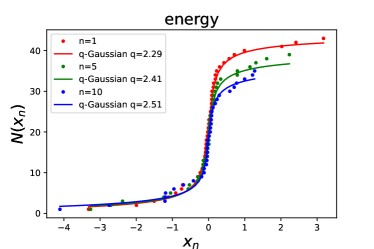
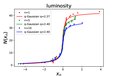
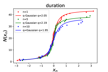
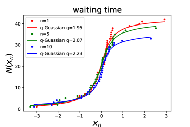
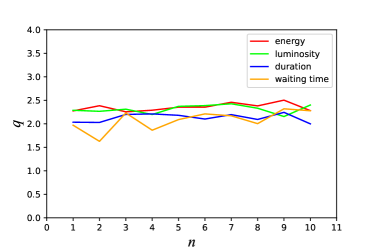
Figure 3 shows some examples of the fits for the high-energy burst sample. In this plot, we display the CDFs of fluctuations of energy (upper-left panel), luminosity (upper-right panel), duration (lower-left panel), and waiting time (lower-right panel) for (red dots), (green dots), and (blue dots). The best fitting -values and the corresponding values for are presented in Table 1. From Figure 3 and the values, we find that the CDFs of fluctuations of energy, luminosity, duration, and waiting time can be well fitted by the CDF of -Gaussian function (see solid curves). Moreover, we plot the best-fitting values as a function of the temporal interval scale in the range , and find that the values also keep approximately steady (see the right panel of Figure 2). The average values of energy, luminosity, duration, and waiting time for the data of high-energy bursts are , , , and , respectively. As shown in Table 2, the values of energy and luminosity (peak flux) of high-energy bursts are consistent with those of FAST observations of low-energy bursts within 1 confidence level, but the values of duration and waiting time between low- and high-energy bursts are significantly different.
One possible explanation for the different values of duration and waiting time for low- and high-energy bursts of FRB 20201124A is that burst duration is subject to instrumental effects, thereby affecting the estimate of the waiting time. It is well known that the observed burst duration would be broadened by instrumental effects (Cordes & McLaughlin, 2003). The instrumental burst broadening includes the intrachannel dispersion smearing and the sampling timescale. The smearing is due to intrachannel dispersion. The time resolution should not be better than the sampling timescale, which broadens the burst. Therefore, different instruments may correspond to different broadening components. However, since we are interested in the statistical distributions of the differences of durations and waiting times at different time intervals, burst broadening induced by instrumental effects can be approximately deducted from subtracting two observed durations (or two waiting times). Thus, we conclude that the different values for low- and high-energy bursts is likely not an instrumental effect. Rather, it more likely hints a differing emission mechanism or emission site between low- and high-energy bursts, although they originate from the same progenitor source.
3 Scale Invariance in Glitching Pulsars
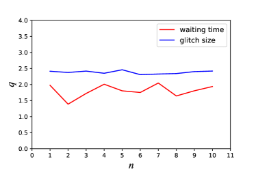
: The best-fitting values in the -Gaussian distribution as a function of .
Remarkably, both a glitch and an antiglitch accompanied by FRB-like bursts from SGR J1935+2154 were recently reported. The temporal coincidences between the glitch/antiglitch and FRB-like bursts imply some physical connection between them (Ge et al., 2022; Younes et al., 2023). The statistical distributions of glitch sizes () and times between successive glitches (waiting times) for some individual pulsars are power-law forms (Morley & Garcia-Pelayo, 1993; Melatos et al., 2008; Carlin & Melatos, 2021). Power-law distributions of energy and waiting time are also found in some repeating FRBs (Wang & Yu, 2017; Katz, 2018; Gourdji et al., 2019; Cheng et al., 2020; Cruces et al., 2021; Li et al., 2021b; Zhang et al., 2021; Hewitt et al., 2022; Jahns et al., 2023; Wang et al., 2023). Inspired by the associations between the glitch/antiglitch and FRB-like bursts of SGR J1935+2154 and the statistical similarities between pulsar glitches and repeating FRBs, here we investigate whether pulsar glitches have a similar scale-invariant behavior.
To date, there are only eight pulsars with more than 10 detected glitches (Fuentes et al., 2019). PSR B1737–30 has been observed regularly by the Jodrell Bank Observatory (JBO), and 37 glitches have been detected over years. PSR B1737–30 has the largest number of glitch events among the glitching pulsars exhibiting power-law size distributions. Consequently, the statistical results for PSR B1737–30 are much more significant than other pulsars. Glitch epochs and sizes for the pulsars are available in the JBO online catalogue (Espinoza et al., 2011)222http://www.jb.man.ac.uk/pulsar/glitches.html. Due to the relatively small sample of glitches, we also focus on the CDFs of fluctuations of glitch size and waiting time at different scale intervals . For a fixed , we use the CDF of -Gaussian (Equation (5)) to fit the CDFs of fluctuations, and derive the best-fitting value. Then we vary and obtain the values as a function of .
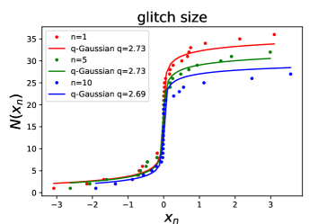
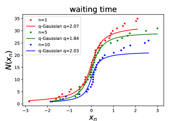
For the detected glitches in PSR B1737–30, the CDFs of fluctuations of glitch size and waiting time are presented in the left and middle panels of Figure 4, respectively. The best-fitting values and the corresponding values for are listed in Table 1. It is clear that the -Gaussian function fits the data points very well. To better highlight the scale-invariant property in PSR B1737–30’ glitches, the best-fitting values as a function of for glitch size and waiting time are plotted in the right panel of Figure 4. Again, we find that the values are nearly constant and independent of . We also list the average values from to 10 for glitch size () and waiting time () in Table 2. Interestingly, the average values of glitch size (energy) and waiting time are well consistent with those of FRB 20201124A’s high-energy bursts, which indicate that there may be an underlying physical connection between pulsar glitches and FRB 20201124A’s high-energy bursts.
4 Summary and discussion
SOC dynamics can be effectively identified and diagnosed by analyzing the avalanche size fluctuations (Caruso et al., 2007). When criticality appears, the PDFs for the avalanche size fluctuations at different times have fat tails with a -Gaussian form. Such a -Gaussian behavior is independent of the time interval adopted, and it is found so when considering energy fluctuations between real earthquakes (Caruso et al., 2007). That is, the values in -Gaussian distributions are nearly invariant for different temporal interval scales, implying a scale-invariant structure in earthquakes (see also Wang et al. 2015). Analogous scale-invariant characteristics have also been discovered in some astronomical phenomena, such as SGRs (Chang et al., 2017; Wei et al., 2021; Sang & Lin, 2022), the repeating FRB 20121102 (Lin & Sang, 2020; Wei et al., 2021), GRB X-ray flares (Wei, 2023) and precursors (Li & Yang, 2023), and gamma-ray flares of the Sun and the blazar 3C 454.3 (Peng et al., 2023). Given the temporal coincidences between the glitch/antiglitch and FRB-like bursts from the Galactic magnetar SGR J1935+2154 (Ge et al., 2022; Younes et al., 2023), here we examined their possible physical connection by comparing the scale-invariant similarities between repeating FRBs and glitching pulsars.
For repeating FRBs, we focused on the statistical properties of the hyperactive repeating source FRB 20201124A using two samples from different observations. The first sample contains 2744 bursts from the FAST observation, and the second one consists of 46 high-energy bursts from the observations of four small 25–32-m class radio telescopes. Note that except for FRB 20121102, it is unclear whether other repeating FRBs share the same scale-invariant property. With the FAST data, we confirmed that the PDFs of fluctuations of energy, peak flux, duration, and waiting time can be well fitted by a -Gaussian function, and the values keep nearly steady for different time scales. Moreover, we found that the average values of energy, peak flux, and duration for the FAST data of FRB 20201124A are very close to those of FRB 20121102 (Wei et al., 2021), which indicate that there is a common scale-invariant feature in repeating FRBs. With the high-energy burst sample, similar scale-invariant results were obtained, but the average values of duration and waiting time of high-energy bursts are significantly different from those of FAST observations of low-energy bursts. This implies that low- and high-energy bursts may originate from different emission mechanisms or emission regions at the progenitor source. Wang et al. (2015) also found that different faulting styles correspond to different values in earthquakes.
For glitching pulsars, we investigated the statistical properties of 37 known glitches from PSR B1737–30. We showed that the distributions of fluctuations of glitch size and waiting time also exhibit a -Gaussian form, with constant values independent of the adopted time scale. This scale-invariant property is very similar to those of repeating FRBs, and both the two astronomical phenomena can be attributed to a SOC process. Interestingly, the average values of glitch size (energy) and waiting time align consistently with those of FRB 20201124A’s high-energy bursts, which suggest that there may be an underlying physical association between pulsar glitches and FRB 20201124A’s high-energy bursts.
In summary, our findings support the argument that both repeating FRBs and pulsar glitches can be explained within a dissipative SOC mechanism with long-range interactions. In the future, much more glitches and FRB-like bursts from the magnetars will be detected. The physical connection between glitches and FRB-like bursts can be further investigated.
References
- Antonopoulou et al. (2022) Antonopoulou, D., Haskell, B., & Espinoza, C. M. 2022, Reports on Progress in Physics, 85, 126901, doi: 10.1088/1361-6633/ac9ced
- Aschwanden (2011) Aschwanden, M. J. 2011, Self-Organized Criticality in Astrophysics
- Aschwanden (2012) —. 2012, A&A, 539, A2, doi: 10.1051/0004-6361/201118237
- Aschwanden (2014) —. 2014, ApJ, 782, 54, doi: 10.1088/0004-637X/782/1/54
- Aschwanden (2015) —. 2015, ApJ, 814, 19, doi: 10.1088/0004-637X/814/1/19
- Aschwanden et al. (2016) Aschwanden, M. J., Crosby, N. B., Dimitropoulou, M., et al. 2016, Space Sci. Rev., 198, 47, doi: 10.1007/s11214-014-0054-6
- Bak et al. (1987) Bak, P., Tang, C., & Wiesenfeld, K. 1987, Physical Review Letters, 59, 381, doi: 10.1103/PhysRevLett.59.381
- Bochenek et al. (2020) Bochenek, C. D., Ravi, V., Belov, K. V., et al. 2020, Nature, 587, 59, doi: 10.1038/s41586-020-2872-x
- Carlin & Melatos (2021) Carlin, J. B., & Melatos, A. 2021, ApJ, 917, 1, doi: 10.3847/1538-4357/ac06a2
- Caruso et al. (2007) Caruso, F., Pluchino, A., Latora, V., Vinciguerra, S., & Rapisarda, A. 2007, Phys. Rev. E, 75, 055101, doi: 10.1103/PhysRevE.75.055101
- Chang et al. (2017) Chang, Z., Lin, H.-N., Sang, Y., & Wang, P. 2017, Chinese Physics C, 41, 065104, doi: 10.1088/1674-1137/41/6/065104
- Cheng et al. (2020) Cheng, Y., Zhang, G. Q., & Wang, F. Y. 2020, MNRAS, 491, 1498, doi: 10.1093/mnras/stz3085
- CHIME/FRB Collaboration et al. (2020a) CHIME/FRB Collaboration, Amiri, M., Andersen, B. C., et al. 2020a, Nature, 582, 351, doi: 10.1038/s41586-020-2398-2
- CHIME/FRB Collaboration et al. (2020b) CHIME/FRB Collaboration, Andersen, B. C., Bandura, K. M., et al. 2020b, Nature, 587, 54, doi: 10.1038/s41586-020-2863-y
- Cordes & McLaughlin (2003) Cordes, J. M., & McLaughlin, M. A. 2003, ApJ, 596, 1142, doi: 10.1086/378231
- Cruces et al. (2021) Cruces, M., Spitler, L. G., Scholz, P., et al. 2021, MNRAS, 500, 448, doi: 10.1093/mnras/staa3223
- Espinoza et al. (2011) Espinoza, C. M., Lyne, A. G., Stappers, B. W., & Kramer, M. 2011, Monthly Notices of the Royal Astronomical Society, 414, 1679, doi: 10.1111/j.1365-2966.2011.18503.x
- Fong et al. (2021) Fong, W.-f., Dong, Y., Leja, J., et al. 2021, ApJ, 919, L23, doi: 10.3847/2041-8213/ac242b
- Foreman-Mackey et al. (2013) Foreman-Mackey, D., Hogg, D. W., Lang, D., & Goodman, J. 2013, PASP, 125, 306, doi: 10.1086/670067
- Freedman & Diaconis (1981) Freedman, D., & Diaconis, P. 1981, Probability Theory and Related Fields, 57, 453, doi: https://doi.org/10.1007/BF01025868
- Fuentes et al. (2019) Fuentes, J. R., Espinoza, C. M., & Reisenegger, A. 2019, A&A, 630, A115, doi: 10.1051/0004-6361/201935939
- Ge et al. (2022) Ge, M., Yang, Y.-P., Lu, F., et al. 2022, arXiv e-prints, arXiv:2211.03246, doi: 10.48550/arXiv.2211.03246
- Good & Chime/Frb Collaboration (2020) Good, D., & Chime/Frb Collaboration. 2020, The Astronomer’s Telegram, 14074, 1
- Gourdji et al. (2019) Gourdji, K., Michilli, D., Spitler, L. G., et al. 2019, ApJ, 877, L19, doi: 10.3847/2041-8213/ab1f8a
- Haskell & Melatos (2015) Haskell, B., & Melatos, A. 2015, International Journal of Modern Physics D, 24, 1530008, doi: 10.1142/S0218271815300086
- Hewitt et al. (2022) Hewitt, D. M., Snelders, M. P., Hessels, J. W. T., et al. 2022, MNRAS, 515, 3577, doi: 10.1093/mnras/stac1960
- Huang & Geng (2014) Huang, Y. F., & Geng, J. J. 2014, ApJ, 782, L20, doi: 10.1088/2041-8205/782/2/L20
- Jahns et al. (2023) Jahns, J. N., Spitler, L. G., Nimmo, K., et al. 2023, MNRAS, 519, 666, doi: 10.1093/mnras/stac3446
- Katz (1986) Katz, J. I. 1986, Journal of Geophysical Research, 91, 10412, doi: 10.1029/jb091ib10p10412
- Katz (2018) Katz, J. I. 2018, MNRAS, 476, 1849, doi: 10.1093/mnras/sty366
- Kirsten et al. (2024) Kirsten, F., Ould-Boukattine, O. S., Herrmann, W., et al. 2024, Nature Astronomy, doi: 10.1038/s41550-023-02153-z
- Lanman et al. (2022) Lanman, A. E., Andersen, B. C., Chawla, P., et al. 2022, ApJ, 927, 59, doi: 10.3847/1538-4357/ac4bc7
- Li et al. (2021a) Li, C. K., Lin, L., Xiong, S. L., et al. 2021a, Nature Astronomy, 5, 378, doi: 10.1038/s41550-021-01302-6
- Li et al. (2021b) Li, D., Wang, P., Zhu, W. W., et al. 2021b, Nature, 598, 267, doi: 10.1038/s41586-021-03878-5
- Li & Yang (2023) Li, X.-J., & Yang, Y.-P. 2023, ApJ, 955, L34, doi: 10.3847/2041-8213/acf12c
- Lin & Sang (2020) Lin, H. N., & Sang, Y. 2020, Monthly Notices of the Royal Astronomical Society, 491, 2156, doi: 10.1093/mnras/stz3149
- Lorimer et al. (2007) Lorimer, D. R., Bailes, M., McLaughlin, M. A., Narkevic, D. J., & Crawford, F. 2007, Science, 318, 777, doi: 10.1126/science.1147532
- Mastrano et al. (2015) Mastrano, A., Suvorov, A. G., & Melatos, A. 2015, MNRAS, 453, 522, doi: 10.1093/mnras/stv1658
- Melatos et al. (2008) Melatos, A., Peralta, C., & Wyithe, J. S. B. 2008, ApJ, 672, 1103, doi: 10.1086/523349
- Mereghetti et al. (2020) Mereghetti, S., Savchenko, V., Ferrigno, C., et al. 2020, ApJ, 898, L29, doi: 10.3847/2041-8213/aba2cf
- Morley & Garcia-Pelayo (1993) Morley, P. D., & Garcia-Pelayo, R. 1993, EPL (Europhysics Letters), 23, 185, doi: 10.1209/0295-5075/23/3/005
- Peng et al. (2023) Peng, F.-K., Wei, J.-J., & Wang, H.-Q. 2023, ApJ, 959, 109, doi: 10.3847/1538-4357/acfcb2
- Petroff et al. (2022) Petroff, E., Hessels, J. W. T., & Lorimer, D. R. 2022, A&A Rev., 30, 2, doi: 10.1007/s00159-022-00139-w
- Piro et al. (2021) Piro, L., Bruni, G., Troja, E., et al. 2021, A&A, 656, L15, doi: 10.1051/0004-6361/202141903
- Rajwade et al. (2020) Rajwade, K. M., Mickaliger, M. B., Stappers, B. W., et al. 2020, MNRAS, 495, 3551, doi: 10.1093/mnras/staa1237
- Ravi et al. (2022) Ravi, V., Law, C. J., Li, D., et al. 2022, MNRAS, 513, 982, doi: 10.1093/mnras/stac465
- Ridnaia et al. (2021) Ridnaia, A., Svinkin, D., Frederiks, D., et al. 2021, Nature Astronomy, 5, 372, doi: 10.1038/s41550-020-01265-0
- Sang & Lin (2022) Sang, Y., & Lin, H.-N. 2022, MNRAS, 510, 1801, doi: 10.1093/mnras/stab3600
- Spitler et al. (2016) Spitler, L. G., Scholz, P., Hessels, J. W. T., et al. 2016, Nature, 531, 202, doi: 10.1038/nature17168
- Tavani et al. (2021) Tavani, M., Casentini, C., Ursi, A., et al. 2021, Nature Astronomy, 5, 401, doi: 10.1038/s41550-020-01276-x
- Thompson et al. (2000) Thompson, C., Duncan, R. C., Woods, P. M., et al. 2000, ApJ, 543, 340, doi: 10.1086/317072
- Tsallis (1988) Tsallis, C. 1988, Journal of Statistical Physics, 52, 479, doi: 10.1007/BF01016429
- Tsallis et al. (1998) Tsallis, C., Mendes, R., & Plastino, A. R. 1998, Physica A Statistical Mechanics and its Applications, 261, 534, doi: 10.1016/S0378-4371(98)00437-3
- Wang et al. (2023) Wang, F. Y., Wu, Q., & Dai, Z. G. 2023, ApJ, 949, L33, doi: 10.3847/2041-8213/acd5d2
- Wang & Yu (2017) Wang, F. Y., & Yu, H. 2017, J. Cosmology Astropart. Phys, 2017, 023, doi: 10.1088/1475-7516/2017/03/023
- Wang et al. (2015) Wang, P., Chang, Z., Wang, H., & Lu, H. 2015, European Physical Journal B, 88, 206, doi: 10.1140/epjb/e2015-60441-6
- Wei (2023) Wei, J.-J. 2023, Physical Review Research, 5, 013019, doi: 10.1103/PhysRevResearch.5.013019
- Wei et al. (2021) Wei, J.-J., Wu, X.-F., Dai, Z.-G., et al. 2021, The Astrophysical Journal, 920, 153, doi: 10.3847/1538-4357/ac2604
- Wu et al. (2023) Wu, Q., Zhao, Z.-Y., & Wang, F.-Y. 2023, MNRAS, 523, 2732, doi: 10.1093/mnras/stad1585
- Xiao et al. (2021) Xiao, D., Wang, F., & Dai, Z. 2021, Science China Physics, Mechanics, and Astronomy, 64, 249501, doi: 10.1007/s11433-020-1661-7
- Xu et al. (2022) Xu, H., Niu, J. R., Chen, P., et al. 2022, Nature, 609, 685, doi: 10.1038/s41586-022-05071-8
- Younes et al. (2023) Younes, G., Baring, M. G., Harding, A. K., et al. 2023, Nature Astronomy, 7, 339, doi: 10.1038/s41550-022-01865-y
- Zhang (2020) Zhang, B. 2020, Nature, 587, 45, doi: 10.1038/s41586-020-2828-1
- Zhang (2023) —. 2023, Reviews of Modern Physics, 95, 035005, doi: 10.1103/RevModPhys.95.035005
- Zhang et al. (2021) Zhang, G. Q., Wang, P., Wu, Q., et al. 2021, ApJ, 920, L23, doi: 10.3847/2041-8213/ac2a3b
- Zhang et al. (2022) Zhang, Y.-K., Wang, P., Feng, Y., et al. 2022, Research in Astronomy and Astrophysics, 22, 124002, doi: 10.1088/1674-4527/ac98f7
- Zhou et al. (2022) Zhou, D. J., Han, J. L., Zhang, B., et al. 2022, Research in Astronomy and Astrophysics, 22, 124001, doi: 10.1088/1674-4527/ac98f8