A Concise Proof of Discrete Jordan Curve Theorem
Abstract
In geometry and graph theory, the Jordan curve theorem has both educational and academic roles. There have been many proofs published in educational journals in mathematics, notably “American Mathematical Monthly.”[16, 17, 18, 19] This paper gives a concise proof of the Jordan curve theorem on discrete surfaces. We also embed the discrete surface in the 2D plane to prove the original version of the Jordan curve theorem. This paper is a simple version of [5]. We seek to clarify and simplify some statements and proofs. Again, the purpose of this paper is to make the proof of the theorems easier to understand. We omit some definitions of concepts, which can be found in [6, 4, 3, 5]. In revision 2, we added another appendix to make a self-contained proof on verifying simple connectedness of the Euclidean plane in this paper. In this revision, we added a special case for the proof of Theorem 3 in Appendix B that was found when we were revising a new paper for high dimensional contraction [7]. It was easy to resolve in 2D. We put it in Appendix C of this paper. 111Readers who do not want to know the details of the concepts in discrete surfaces can begin in Section 2 to get an idea of the proofs based on the intuitive meaning of the concepts used in this paper.
1 What is the Jordan Curve Theorem?
In this paper, we give a straightforward proof of the Jordan curve theorem in 2D discrete spaces with respect to the general definition of discrete curves, surfaces, and manifolds discussed in [1, 6]. The Jordan curve theorem states that a simple and closed curve separates a simply connected surface into two components. Based on the definition of discrete surfaces, we give three reasonable definitions of simply connected spaces in discrete spaces. Theoretically, these three definitions are equivalent.
For the Jordan curve theorem, O. Veblen in 1905 wrote a paper [13] that was regraded as the first correct proof of this fundamental theorem on 2D Euclidean plane. The first discrete proof was given by W.T. Tutte on planar graphs in 1979 [14]. Recently, researchers still show considerable interests in the Jordan curve theorem using formalized proofs in computers [15].
In 1999, L. Chen attempted to prove the discrete Jordan curve theorem for 2D discrete manifolds without using 2D Euclidean space [3]. Chen added some missing parts of this proofs in 2013 [5]. In [5], Chen adopted some original ideas from Veblen’s paper and gave a proof of this theorem in discrete form.
In this paper, we want to give a simple and easy version of the proofs given in [5] without gone through many definitions of discrete geometry.
A discrete surface can be viewed as a digital surface or a triangulated 2D meshes. Intuitively, a discrete 2-cell in this paper is a smallest or minimal unite for 2D objects. A discrete 2-cell cannot be slitted into two other 2-cells. The union of two (discrete) 2-cells , and will not be a two cell if . (In discrete space, an object is mainly formed by vertices or points. The others such as edges, faces are based on human’s interpretation.) In other words, the smallest unite does not contain any other 2-cell. When we say a 2-cell, we need to think this “thing” as the smallest one containing some vertices and edges. Please note that this definition is different from the standard definition in topology.
We know that a discrete surface can be naturally embedded to Euclidean plane or a closed continuous surface such as a sphere. Indeed, a discrete surface can be easily embedded to a 3D or higher dimensional Euclidean spaces.
Let us first review some concepts of discrete curves in [3, 6]: (1) A simple path is called a (discrete) pseudo-curve, (2) a simple semi-curve can be a curve or a surface-cell (2-cell) (in discrete form, a set containing all vertices means that the set contains all 2-cell in this set. At least it is true for this paper. See details in [6] for general non simply connected surfaces.) (3) A simple curve must not contain any proper subset that is a 2-cell.
It is obvious, if we define a simple path (a pseudo-curve in this paper) a discrete curve, there is no Jordan Curve theorem in discrete space. This is because that the inner part of a 2-cell is empty in graph-structures. This little difference will not affect the continuous version of the theorem. In discrete cases, we will make a point called “the Veblen point” to deal with this when we desire a closer version of the theorem to the continuous case.
We defined regular points in a discrete manifolds in [6]. It just means that every point on surface has a neighborhood that is similar to a 2D disk (homeomorphic equivalence in topology).
Let be the neighborhood of in . If is a triangulated surface, then
or where is graph-distance. For any type of discrete surfaces, .
We proved that for a discrete surface , if is a inner and regular point of , then there exists a simple cycle containing all points in in . This result is particularly important in our proof, but it is very intuitive too. We present this result as Lemma 1 [6, 5].
Lemma 1
For a discrete surface , if is a inner and regular point of , then there exists a simple cycle containing all points in in where is the neighborhood of in .
In topology, the formal description of the Jordan curve theorem is: A simply closed curve in a plane decomposes into two components. [11, 12] In fact, this theorem holds for any simply connected 2D surface. A plane is a simply connected surface in Euclidean space, but this theorem is not true for a general continuous surface. For example, the boundary of a donut.
We now introduce the meaning of discrete deformation and simply connected discrete surfaces.
What is a simply connected continuous surface? A connected topological space is simply connected if for any point in , any simply closed curve containing can be contracted to . The contraction is a continuous mapping among a series of closed continuous curves. [12] So, we first need the concept of “discrete contraction.”
Here we also try to make the definition of simply connected discrete surfaces to be simpler. The more detailed definition was in [4, 6].
The “contraction” means the sequence of curves will be getting smaller and smaller until they shrink to a point. These curves do not cross each other. (They do not have to be cross each other. This is a key too.)
So our concept of contraction is that a discrete curve will be graduate varied to a “smaller” one, and keep the process until “shrink” to a point. These discrete curves do not cross each other. they can share some points.
In order to keep the concepts simple to understand, we defined the gradual variation between two simple paths in [6, 4, 5]. We defined discrete deformation among discrete pseudo curves. And finally, we define the contraction of curves is a type of discrete deformation. See [6, 4] for more details of the definitions. The reader can just use the natural interpretation of definitions. In paper, we assume the discrete surface is both regular and orientable too. The algorithm to decide if a discrete surface is orientable can be found in [6].
Intuitively, two simple paths and are said to be gradually varied if there is no hole in between and . In addition, there is no jump from to .
More formally, two simple paths and are called gradually varied if consists of 1-cells and 2-cells where no cycle in that is not a 2-cell or the union of 2-cells. In other words, Assume denotes all edges in path . Let . is called in Newman’s book [12]. and are gradually varied iff are the union of 2-cells.
To prove the Jordan curve theorem, we need to describe what the disconnected components are by means of separated from a simple curve ? It means that any path from a component to another must include at least a point in . It also means that this linking path must cross-over the curve . We will define the concept of “cross-over” in the following.
Because a surface-cell is a closed path, we can define two orientations (normals ) to : clockwise and counter-clockwise. Usually, the orientation of a 2-cell is not a critical issue. However, for the proof of the Jordan curve theorem it is necessary.
In other words, a pseudo-curve which is a set of points has no “direction,” but as a path , it has its own “travel direction” from to .
For two paths and , which are gradually varied, if a 2-cell is in , the orientation of with respect to is determined by the first pair of points and . Moreover, if a 1-cell of is in , then the orientation of is fixed with respect to .
According to Lemma 1, contains all adjacent points of and is a simple cycle—there is a cycle containing all points in .
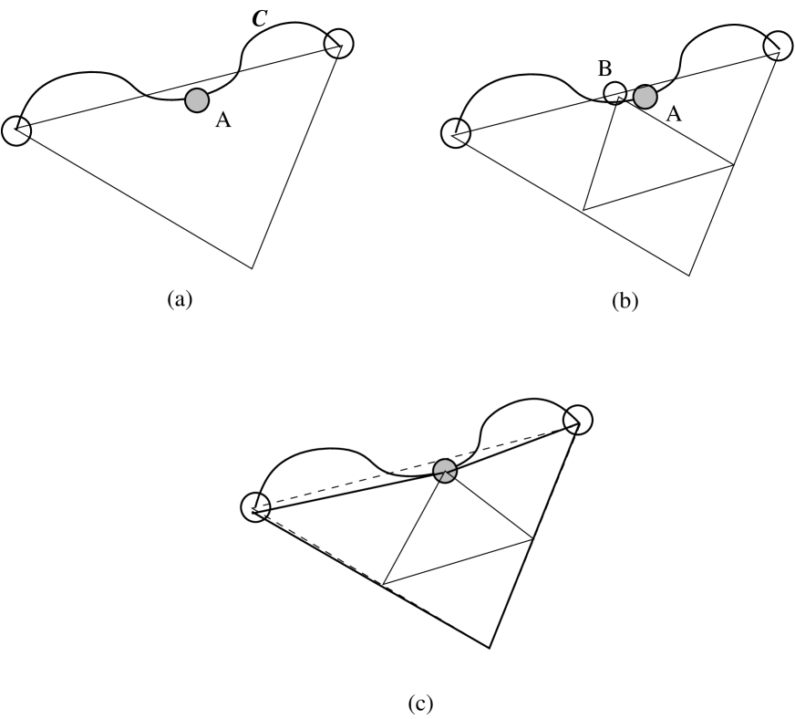
We assume that cycle is always oriented clockwise. For two points , there are two simple cycles containing the path : (1) a cycle from to to then moving clockwise to , and (2) a cycle from to to then moving counter-clockwise to . See Fig. 1(a).
It is easy to see that the simple cycle separates into at least two connected components because from to any other points in the path must contain a point in . is an example the Jordan curve.
Definition 1
Two simple paths and are said to be “cross-over” each other if there are points and ( may be the same as ) such that and where and . The cycle without in and the cycle without in have different orientations with respect to .
For example, in Fig. 1 (b), and are “cross-over” each other. When and are not “cross-over” each other, we will say that is at a side of . We also say that and in the above Lemma are side-gradually varied.
Lemma 2
If two simple paths and are not cross-over each other, and they are gradually varied, then every surface-cell in has the same orientation with respect to the “travel direction” of and opposite to the “travel direction” of .
Intuitively, a simply connected set is such a set so that for any point, every simple cycle containing this point can contract to the point.
Definition 2
A simple cycle can contract to a point if there exist a series of simple cycle, : (1) contains for all ; (2) If is not in then is not in all , ; (3) and are side-gradually varied.
We now show three reasonable definitions of simply connected spaces below. We will provide a proof for the Jordan curve theorem under the third definition of simply connected spaces. The Jordan theorem shows the relationship among an object, its boundary, and its outside area.
Let be a subset of all minimal closed curves on . Each element in is a 2-cell. defines a 2D topological structure discretely.
A general definition of a simply connected space should be :
Definition 3
Simply Connected Surface Definition (a) is simply connected if any two closed simple paths are homotopic.
If we use this definition, then we may need an extremely long proof for the Jordan curve theorem. The next one is the standard definition which is the special case of the Definition 3. (Definition 3 is too general, it is not needed here.)
Definition 4
Simply Connected Surface Definition (b) A connected discrete space is simply connected if for any point , every simple cycle containing can contract to .
This definition of the simply connected set is based on the original meaning of simple contraction. In order to make the task of proving the Jordan theorem simpler, we give the third strict definition of simply connected surfaces as follows.
We know that a simple closed path (simple cycle) has at least three vertices in a simple graph. This is true for a discrete curve in a simply connected surface . For simplicity, we call an unclosed path an arc. Assume is a simple cycle with clockwise orientation. Let two distinct points . Let be an arc of from to in a clockwise direction, and be the arc from to also in a clockwise direction, then we know . We use to represent the counter-clockwise arc from to . Indeed, . We always assume that is in clockwise orientation.
Definition 5
Simply Connected Surface Definition (c) A connected discrete space is simply connected if for any simple cycle and two points , there exists a sequence of simple cycle paths where and such that and are side-gradually varied for all .
We have proved the following proposition in [5].
Proposition 1
Definition (b) and Definition (c) are equivalent.
2 The Jordan Curve Theorem in Discrete Space
Since a simple cycle is a closed simple path that could be a surface-cell that cannot separate into two disconnected components. So for the strict case of Jordan curve theorem, we must use the closed discrete curve (not only a simple cycle).
A discrete curve does not contain a subset of vertices that are not all vertices of a 2 cell in . The intuitive meaning is that does not contain any 2-cell.
A 2-cell will have two directions: the clockwise and the counter-clockwise. If we imagine a point at the center of 2-cell, we will have two normals. (This is also true for 1-cell) This point will be called the central pseudo point. In the case of allowing the central pseudo points that will be called the Veblen point, we will have the general Jordan Curve Theorem. We will prove this case at the last of this section. The idea of the central pseudo point is valid when embedding a surface (or cells) into Euclidean space.
The proof of The Jordan Curve Theorem in Discrete Space will need to use the following proposition:
Lemma 3
If is an edge, define . Then, is a simple path.
We can let , and we denote . However, this lemma is not true when is a discrete curve, . In general,
Lemma 4
is a degenerated (closed) simple path.
A degenerated (closed) path is a simple path with several unclosed discrete curve attach to some vertices on the path. This is because, in discrete case, some part of the simple path shrink or folded into a poly-line.
When every “angle” in a discrete curve is little wide meaning that contains three 2-cells. In other words, for each three consecutive points in , a path from to without passing , there are must be two other vertices in between. In addition, these two vertices are in a 2-cell or more 2-cells that does not contain nor . This means that there is a 2-cell in between the neighborhoods of and .
We also request any two vertices that are not adjacent will have the graph-distance greater than 2. The purpose is to guarantee that is a simple closed path.
We denote the wideness of an angle is the minimum number of edges in the path from to (each edge is in different 2-cell containing ). Note that an angle with wideness 1 will make that is not a discrete curve. Since contains a triangle that is a 2-cell.)
Lemma 5
Let be a discrete curve and be a path (arc) in . ( and are separated by at least three 2-cells.)
If the following conditions are satisfied:
(1) The wideness of each angle is 3 or greater, and
(2) For any two nonadjacent vertices and in , any path not including edges in from to much contain three edges that belong to three different
2-cells.
then, is a closed simple path.
We will prove this lemma in the proof of Theorem 1.
We know that we can easily make in 2D Euclidean plane to be a wide angle by adding some lines to the Veblen points on a edge. (Do not make extra Veblen point used just for a 2-cell, use it for the 2-cell that share the Veblen point.)
The following theorem is for with the wider angles. To direct prove this theorem for general case meaning allowing that is a degenerated (closed) simple path. We will give the proof in Appendix.
For a closed discrete curve, we have
Theorem 2.1
(The Jordan Curve Theorem in Discrete Space) A discrete simply connected surfaces defined by Definition 5 (Definition (c)), has the Jordan property: For a closed discrete curve on , if does not contain any point of , divides into at least two disconnected components. In other words, consists of at least two disconnected components.
Proof
Suppose that is a closed curve in a simply connected surface . does not reach the border of , i.e. .
We also check if it satisfies the condition of the wide angle for each triple consecutive vertices.
Also we add Veblen points and edges to make to be wide as necessary. So we can assume that:
(1) The wideness of each angle is 3 or greater, and
(2) For any two nonadjacent vertices and in , any path not including edges in from to much contain three edges that belong to three different
2-cells.
Assume point , then suppose that and are two adjacent points of in with form of , where the direction of … to to …to is clockwise. See Fig. 2 is a line-cell, then there are two 2-cells containing . Denote these 2-cells by and with clockwise orientation.
Our strategy is to prove that if there is a point in which is not in , and a point and , then any path from to must contain a point in . Then we can see that are not (point-) connected and we have the Jordan curve theorem.
First, we want to prove that there must exist a point in . If each point in is in , since is a simple cycle, then . However, is not a surface-cell, so the statement can not be true. Thus, there is a point . For the same reason there is a point . We assume that is the last such point in starting with , and is the first such point in starting with . (see Fig. 2(a)) We always assume clockwise direction here for cell and unless we indicate otherwise.
Let us make a summery of above idea: Suppose that is a closed curve. (If is a closed simple path, we allow is a 2-cell and we allow to assign a pseudo-point in the center of the 2-cell, we still can prove this theorem.) The idea of the proof is to find two points in each sides of the curve . This is because that for any 1-cell in , there are two 2-cells , sharing by the discrete surface definition. must contain a vertex and must contain , and they are not in . , are adjacent to some points in , respectively. We are going to prove that from to , any path must cross-over . That is the most important part of the Jordan curve theorem.
We assume, on the contrary, there is a simple path from to does not cross-over , called in Fig. 2 (a). But we know there is in ( i.e. ) does cross-over . is a cycle in clockwise. (Fig. 2 (a) )
We know is the neighborhood of in . So contains all 2-cells containing . The boundary of is a simple closed curve. (This is because we always assume that is a regular point). is on the boundary of . (The boundary of is ). is a subset of .
We now prove that is not a subset of ; otherwise, it must cross-over . (a 2-cell containing must have an edge on , or all points of the 2-cell are on the boundary of except ). If does not contain , must be a part of boundary of which is a cycle. has two adjacent points on , (If they are not pseudo points, meaning here it can be eliminated or added on an edge that does not affect to the 2-cell) so these two points are also in the boundary of . So there are only two paths from to on the boundary of . These two points are not on the same side of the cross-over path containing . (The boundary of was separated by the cross-over path containing .) must contain such a point that is on .
Therefore we proved is not a subset of . Then is a simple closed curve. ( passes ). By the definition of the simply-connected surface, there are finite numbers of paths ,…, , such that so that and are (side-)gradually varied.
In addition, is gradually varied to (a reversed that passes ).
We now can assume that there is a smallest such that cross over , but does not. (Fig. 2(a) ). We will prove that is impossible if does not cross over .
Let point in and . There are two cases: (1) cross over at a single point on , or (2) cross over at a sequence of points on . We will prove these two cases, respectively.
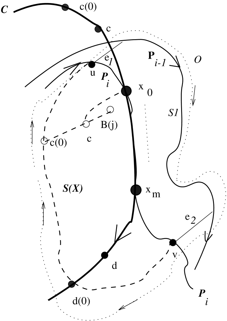
Case 1: Suppose that in Definition 1 (See Fig. 1 (a)(b)). It means two curves and share just one point . and assume and , where .
We know that are in the boundary of , a simple cycle (See Lemma 1). There is a 2-cell (in between and ) contains . See Fig. 2 (b).
has a sequence of points in and a sequence of points in . has at most two edges , not in ; , , , , are the boundary of . is the edge linking to , and is the edge linking to counterclockwise.(Again, may or may not be directly incident to , and may be an empty edge if intersects at point . may also in the same situation.) We might as well assume that is the first point on (from to in path )that is in . Thus, . (If is in must be in . if is in , is not only the cross over point. )
If contains , we will have a cycle in the boundary of contains only points in and , (that are possible end points of , ). is on the boundary of too. Where is ? It must be in the boundary curves (of ) from to or the curve from to . Then in must in the same side of which is part of . Therefore, and do not cross-over each other at . See Fig. 2(b) and the following extended figure.
If does not contain , then there must be a 2-cell (in between and ) containing . We can see that and are line-connected in . (See Fig. 2(c) and above extended figure.) This is due to the definition of regular point of , all surface-cells containing are line-connected. Meaning there is a 2-cell paths they share a 1-cell in adjacent pairs.
Since and are line-connected, we can assume:
a) and share a 1-cell, i.e. . Then is on . Let be the possible edge from to . ( could be empty as ) and is on the boundary cycle of . Except and , is on . is part of the boundary cycle of . In addition, (that is not in ) must be in the boundary curves (of ) from to or the curve from to . Again, in must in the same side of which is part of . Therefore, and do not cross-over each other at . (See Fig. 2(c) also see the above extended figure Fig. 3(c).)
b) and share the point , and there are line-connected 2-cells as a path in between and . . Let us assume that incident to at ( is if is empty ) and incident to at . We will have a set of points in . Each is contained in a 2-cell containing . All are in the boundary cycle of . that is not in . must be in the boundary curves (of ) from to or the curve from to . Thus, in must in the same side of which is part of . and do not cross-over each other at . (See Fig. 2 (c) and Fig. 3(c).)
Case 2: Suppose and cross over a sequence of points on : and , where .
We still have and where and are on for some . Each , , is in a 2-cell that containing some , .
Note that : If does not have a direct edge linking to , will be in a 2-cell between and , either is a pseudo point on for the deformation from to , or and intersects at . That is a pseudo point means here it has a neighbor that has an edge link to , or the neighbor’s neighbor, and so on. We can just assume here is the point that is adjacent to a point in . In the theory, as long as is contained by a 2-cell such that all the points in the 2-cell are in or .

The same way will apply to this case just treat ,…, to in Case 1. We first get the union of ,…,. We want to prove that : The boundary of this union will be simple cycle too under the condition of Lemma 5.
Using mathematical induction we can prove it. After that, we can prove the rest of theorem using the same method presented in Case 1. See Fig. 4.
The following is the detailed proof: Let .
First, we will prove that the boundary of is a simple cycle (it is a simple closed curve too). We know that is an edge in . Also, there are two 2-cells in containing .
is a boundary point in , so no other 2-cell will contain . In the same way, also contains , and is only contained in two 2-cells in . Therefore, and .
Note that and are adjacent 2-cells. On the other hand, is on the boundary curve (that is closed) of . So has two adjacent points on this cycle, and . (We assume that and are not pseudo points, so) and are both on the boundary of . (If or is pseudo points, we can ignore or to find the a actual point that adjacent to .) has two 2-cells containing in . For instance, in Fig. 4 (a) , and contain and and contain . Thus, the boundary of is a closed curve that is formed by the arc from to in the boundary of , plus the arc from to in the boundary of .
Second, we assume the boundary of is a closed curve, when we consider the arc in , we can prove the boundary of is also a closed curve.
We know that we have two closed curves: Suppose that is the boundary of , and is the boundary of . is in , and is in . There are two 2-cells , containing in .
is on the boundary cycle of , then must have two adjacent points in , , and . and are two edges in . In the same way above, we will have the cycle passing and that is the boundary curve of . This is because there is a 2-cell in between the neighborhoods of and as assumed by the wider angle on each point on , is not a folding point, so are . In other words, the point that enters in counterclockwise in differs from the point follows in counterclockwise in .
Thus, we have proved that the boundary curve of is a simple closed curve. In the rest of the proof, we will treat to be in Case 1. See Fig. 5. We now use denote and is an arc in . (Please note that in Case 1, was used as a 2-cell. Now is an arc in . )

In the rest of the proof, we will prove: if and are not cross over each other, then, and will not be cross over each other. Therefore, any must cross over . This completes the proof of the discrete Jordan curve theorem.
Let us first state again that passes but does not contain any point of . In addition, and is gradually varied, i.e. was deformed from directly. We also know that is the neighborhood of the arc in , i.e. the arc is a part of the closed curve . The boundary of is a closed curve too.
are on the boundary of (Assume are not pseudo points, otherwise, we can find corresponding none-pseudo on the boundary of .) is a part of We also know that and are not in . There will be two 2-cells, and , are in between and (all points of and are in ) such that and .
Let and . Let be the edge in linking to (in most cases, incident to , but not necessarily ), and let be the edge in linking to (possibly starting at ). So, are the boundary of , counterclockwise.
Subcase (i): If contains (), all points in ’s boundary are contained in by the definition of . we will have a cycle in the boundary of . is on the boundary of too. But . It must be in the boundary curves (of ) from to or the curve from to . Then in must in the same side of which is part of . Therefore, and do not cross-over each other at . (See Fig. 5.)
Subcase (ii): If does not contain , then there must be a 2-cell (in between and ) containing .
Let be the edge in incident to a point in and a point in , respectively. (In most cases, incident to , i.e. , but not necessarily ). And let be the edge in incident to a point in and a point in , respectively. is usually .
Note that: must not be in . Gradual variation (direct deformation) means that each point in each 2-cell of and in between and must be in . Formally, is a set of 2-cells; every point in these 2-cells is in .
We can see that and are line-connected in by the definition of line-connected paths, meaning there is a path of 2-cells where each adjacent pair shares a 1-cell. (See Fig. 4(d) and Fig. 5.)
From to , there is an arc in . To prove that all points in this arc are in the boundary of we need to prove each point on the arc must be in a 2-cell that contains a point in , and this 2-cell is other than (except this 2-cell is) or . It gives us some difficult to prove it. The above discussion seems not very productive.
We found a more elegant way to prove this case by finding another simple path (or pseudo curve) that cross-over . The method is the following: If , there must be a in , has an edge linking to . (Otherwise, are in a 2-cell that contains some points in . Therefore, .) We can also assume that is not , otherwise, is in , so . See Fig. 6.
We select the smallest having an edge linking to , . is in both and . We might as well let is such an edge, and is a point in . Therefore, we will have the new path (simple path), . This new path has two parts: The first part is the same as before and including the point , and the second part is the partial path (curve) of after point . This path does cross-over . It is obvious that are gradually varied. This is because we just inserted a path in between of and .
This new path has such a good property that is do not incident (link) an edge that has an end vertex in . Since is in , the 2-cell (in 222Here is exclusive “OR” operation defined in [6], just like in [12] ) contains also contains and (in ). Since no edge from to , containing is just . We will have just Subcase (i) using to replace .
The entire theorem is proven. ∎
3 The Jordan Curve Theorem for Generalized Simple Closed Paths
The discrete Jordan curve theorem proved in last section has a little difference from the classical description of The Jordan curve Theorem. This is because that discrete curve has its own strict property: does not contain any 2-cell. In order to satisfy the classical form. We need to use central pseudo points, we call it the Veblen point, for each type of cells, especially 1-cells (line-cells) and 2-cells (surface-cells) So we will allow the simple path (semi-curve) in the proof of the Jordan curve theorem. In fact, a little modification will assist the proving of the theorem. The rest of work is just to prove that there are only two (connected) components in .
A 2-cell in this paper is a small unite, the smallest unite that does not contain any other 2-cell. A 2-cell in discrete space contains a central pseudo point that is called the Veblen point in this paper. At this point, we can define two normals, one is in clockwise direction and another is is on counterclockwise direction. We can realize it in Euclidean plane.
Theorem 3.1
(The Jordan Curve Theorem for Generalized Simple Closed Paths) Let be a discrete simply connected surfaces, ( can be closed or a discrete plane embedded in 2D Euclidean Space). A closed simple path (0-cell connected semi-curve) which does not contain any point of divides into two components (in terms of allowing central pseudo points for each cell). In other words, consists of two components. These two components are disconnected.
Proof
In this proof, we can put the central pseudo points (the Veblen points) for each 1-cells and 2-cells to assist our proof. The reason is that if we embed 1-cells and 2-cells into Euclidean plane or higher dimensional space. We can always find the central points for each cell. The idea of the central pseudo points is at least valid in Euclidean space. In fact, the central pseudo points also have two normal directions for a 2-cell. It also has two directions for a 1-cell. For instance, is an edge, and are two directions.
In the proof of Theorem 1, we know that we have two 2-cells and at the different side of the cycle . We proved that point and are not connected in .
has the orientation of clockwise (or counterclockwise as we first made). is clockwise in , but is counterclockwise in . So we call is clockwise, and is counterclockwise. For each edge (e.g. ) in , we will have two 2-cells containing , denoted by and . There must be one in clockwise and another is in counterclockwise.
We always assume that is clockwise and is counterclockwise. We now add all the central pseudo points to all 1-cells and 2-cells in . And immediately remove all central pseudo points from 1-cells in . (This operation is to stop a path will go through the central pseudo points on .)
We also know in our assumption: each 2-cell must have at least three edges (1-cells) in its boundary. This is because is a simple graph. (We can always add a point to make it in Euclidean space.) We also assume that does not reach the border of meaning that .
Case 1: A special case is the boundary of a single 2-cell, denoted as . A simple path could be just the boundary of a 2-cell. In this case, we have a central pseudo point in the cell . So this theorem is virtually true if we can prove that is point-connected. That is to say that except the central pseudo point in , is a point-connected component. In other word, is one point-connected component.
We can prove this is because of the following facts: For each cell in , if has an edge in . The boundary of is a simple closed path. If the boundary of is , then since every edge has shared by two 2-cells ( and ) already. We have two components in : the central pseudo point of and the central pseudo point of .
Case 2: The general case
We know 2-cells that are joint with an edge in have two types: the clockwise type, denoted as , , , and the counterclockwise type, denoted as , , .
We can prove that all are connected without using points in . This is because that any point in is contained by two 1-cells and in . These two 1-cells are contained by and , respectively. If , it is connected. If A If and share an edge, then, the central pseudo points of and are connected. If and do not share an edge, we know and are in , there must be a cycle contains some edges in and some edges of , and . So and are connected (meaning through their central pseudo points ) do not pass . Therefore, all ’s (meaning using their central pseudo points) are connected. In other words, split into two parts, one called include and , and another one, include some ’s. and are point connected in without passing any point in . All cells that are not or in will also assign as the clockwise type, i.e. for some . So all ’s are connected.
In the same way, we can prove that all ’s are connected. ( .)
We now prove that any point in , must be connected to the component containing or to the component containing . We know that any two points are point-connected by a path in . Let , is such a path connecting and . Note that every point in is contained by . Since is not in , (which has finite numbers of points) must contain the first point in , we assume it is . In many cases, . Let . Then must be not in . Thus, must be in . must be in some or because .
In other words, there must be a first point in , , that is adjacent a point ( may or may not be point ). must belong to an or . So if belong to , is a point connected to the central pseudo points of . We call it component . All points in are connected since are connected for all .
If belong to , is a point connected to the central pseudo points of . We call it component . All points in are connected since are connected for all . We also know since was selected from .
According to the proof of on Theorem 1, there is in some is not connected to in some in . is in , and in . Therefore, any point in is not connected to any point in in in . (Otherwise, will be connected to that point in , then will be connected to any point in .)
We now complete the proof of Theorem 2, the general Jordan Curve Theorem. ∎
4 Subdivision of Triangles and Jordan Curve Theorem in Euclidean Space
In Theorem 2, we allow the simple path (pseudo-curves) for the Jordan Curve Theorem. This is the general case of Jordan Curve Theorem in discrete space. We know that 2D Euclidean space can be partitioned into triangles and it is simply connected in this discrete space in terms of simplicial complexes. So we can prove the Jordan Curve Theorem for 2D Euclidean plane.
The only problem is that we need to assume that we have a refinement process that will make the triangulation (joint with the simple curve ) infinitively approximates .
The following construction will bring a more satisfied answer. We will use the mid point subdivision method to refine a triangulation. Even though we can use barycentric subdivision to refine a triangle, but it is computationally expensive. In the following figure, the mid point subdivision method will partition the triangle into four small triangles if we agree a curve can be represented as , . then we can get , And so on so fourth.
Algorithm 1 The mid point subdivision method to partition a triangle along with the boundary curve .
Step 1: The curve joints with a triangle at two points. (Fig. 7 (a))
Step 2: Subdivision of the triangle using the mid point method. The mid point of the edge joining with in triangle is not exactly on the mid point of the arc of . (Fig. 7 (b))
Step 3: Make the two mid points as one on the curve . And modify the subdivision triangle accordingly. (Fig. 7 (c))
(This algorithm might not be a new algorithm. It is a natural way to do it. If someone already found this algorithm, We will cite his/her work.)
If the close (boundary) curve is a continuous curve, the process of making the mid point subdivision is always valid. This process is only for the approximating that will cover all points. This theorem is valid for the point of approximation. For any , we can find a triangulation where the length of each edge is smaller than , and the vertices on the boundary (in discrete term are the points on the curve .
There is no way to link outside of the without passing . separates the plane into two components. is infinitively close to . So the theorem is proven in the continuous case.
The second method could be the following: Can we define a line with with, then we can make the line thinner and thinner to approximate the answer? What we can state is that for any and , we can find a that is the approximation of with respect to . Each edge is shorter than .
(A mapping from to , and the distance between two adjacent points on is bounded by a bounded function of since is continuous)
So we can prove that every curve with width , from inside of curve to outside of curve , must pass a vertex in . We already proved this. When goes infinitively small, we have this theorem proved. This is one way of thinking.
The Jordan Curve Theorem might only have some “approximation” proofs
along with the progress of mathematics. However, for a safe part, finite and discrete proofs of this great theorem is
very important.
Acknowledgment The author would like to express many thanks to Professors Feng Luo and Xiaojun Huang at Rutgers University.
They have provided many helpful comments. Dr. Luo mentioned a result on triangled surfaces: It stats that every two poly-line are deformable to
each other by using a sequence of poly-lines where each pair of adjacent two only differs by a triangle. If this result is directly used
the proof of Theorem 1 in this paper, the proof would be much easier for a triangulated surface. Due to the nature of the difficulty of the
proofs on the Jordan curve theorem historically, the author will hold total responsibility of this paper when an error occurs in the paper.
5 Appendix A: The Direct Proof of JCT in Discrete Cases
The following is the proof of Theorem 1 without adding any new 2-cells for avoiding a degenerate simple path. In other words, we allow that is a degenerate simple path in the direct proof.
We have add some 2-cells in order to preserve the boundary cycle of in Lemma 5 and Theorem 1. However, the Jordan curve theorem is true for the any closed discrete curve on surface defined in this paper.
Recall the boundary of , . We can say that even though might not be a closed simple path. But it is a degenerate simple path (Fig. 8)

Our purpose is to prove that the point in Fig.2(a) is on the cycle not on the branch of , or there is a point on that has the similar functionality like . Therefore, we can still make the same statement as it in the proof of Theorem 1.
In the proof of Lemma 5, we can see for general case, might be a folding point since it is possible that ’s boundary attached with the boundary of . See Fig. 4 (b) and (d). We let for convenience later.
There are two cases we are interested in: (1) is the last point of branch point respect to , (2) is the middle point of branch point . If is on the cycle (the first point of to is also in ), we will use this case in the current proof which will be similar to the proof in Theorem 1.
Case 1: If is the last point of branch point , we know that the last point of branch (which is ) is adjacent to a in , . since is also adjacent to . So is already a cycle. So . This is not possible since we only consider is at most having points when considering cell and , there is an edge on not in . See Fig. 2. (a).
Case 2: If is in the middle of , there is an edge containing in toward to on , the first point on . There are two 2-cells ( and) containing this edge in . On the other hand, has two neighbors in : one is another denotes . Consider , and are also in . See Fig. 9. , we only have four possible subcases. is not reachable for in Fig (b) and (c), and is not reachable from in Fig. 9 (a) and (d). By the definition of and , they are 2-cells that contain a point in . Therefore, must be on . If is not , we can do it again to find in that is also on . So on so forth, we will have one point on that is . is on . Please note: are in .

We have proved that there is a point (it was denoted as ) near , is on . ( is in the most time). The same thing will be true for , denote the points as . In , from to , every point is in as we proved above. Therefore the situation is exactly the same as we discussed in the proof of Theorem 1.
Up to now we should be able to declare that we have proved completely Theorem 1 without adding any extra 2-cells in the proof of Theorem 1.
In order to walk through the whole proof with each small detail. We now repeat the proof of the case where () as in Theorem 1.
In the rest of the proof, we will prove: If and are not cross over each other, then, and will not be cross over each other. Therefore, any must cross over . This completes the proof of the discrete Jordan curve theorem.
Let us first state again that passes but does not contain any point of . In addition, and is gradually varied, i.e. was deformed from directly. We also know that is the neighborhood of the arc in , i.e. the arc is a part of the closed curve . The boundary of is a degenerate simple path shown in Fig. 8.
are on the boundary of (Assume are not pseudo points meaning only have two neighboring points in , otherwise, we can find corresponding none-pseudo on the boundary of .) is a part of We also know that and are not in . There will be two 2-cells, and , are in between and (all points of and are in ) such that and .
Let and . Let be the edge in linking to (in most cases, incident to , but not necessarily ), and let be the edge in linking to (possibly starting at ). So, are the boundary of , counterclockwise.
Subcase (i): If contains (), all points in ’s boundary are contained in by the definition of (since ). we will have a cycle in the boundary of .
and are on the boundary of too. Especially, is on in (See Fig. 8). In addition, in is in . But . (and ) must be in the boundary path of from to or from to . is on . So if is in between to , see Fig. 10, then (an arc in ) in must be in the same side of which is part of . The same reason will apply to the case that is in between to . Please also note that and are in the boundary (degenerate) path as shown in Fig. 8 not necessary on . Therefore, and do not cross-over each other at . (See Fig. 10.)
Subcase (ii): If does not contain , then there must be a 2-cell (in between and ) containing . We still want to find another simple path (or pseudo curve) that cross-over in between and . And between and , there is only 2-cell just like Subcase (i). The construction method is exactly the same as Subcase (ii) in the proof of Theorem 1 in Section 2. Therefore, we can obtain the case is just like Subcase (i) above. The proof is completed.
6 Appendix B: Simply Connected Space and the Euclidean Plane
In this appendix, we will prove that the Euclidean plane is simply connected under our definition. As a by-product, this proof will also prove the Jordan–Schoenflies theorem.
The Jordan–Schoenflies theorem states that: A simple closed curve on the Euclidean plane separate the plane into two connected components. The component with bounded closure is homeomorphic to the disk.
For a given simple polygon in the plane , our proof is to make a standard triangulation (the equilateral triangle partition) on the plane. That will dense enough such that there is no two and more vertices of are inside of a triangle or an edge. Then we modify the triangulation so that will be the boundary of the triangulation. Then, we design an algorithm that will do contraction of to any given point on . This contraction is a sequence of side-gradually varied paths. So we can prove is simply connected under our definition of this paper.
Since each step of contraction only differs by one triangle in the process. The homeomorphic mapping from inside of that contains finite number of triangles. They have a sequence of homeomorphic mappings from one to its neighbor in contraction (adding a triangle) . We will end up with a final triangle that is homeomorphic to a disk. So we complete the proof.
The key part of this proof is to construct an algorithm: We use the graph-distance for the construction of contraction sequence.
Theorem 6.1
(Simple Connectedness of the Euclidean Plane) The Euclidean Plane is simply connected.
Proof
(According to the definition of the simple connectedness, we want to prove that each simple closed curve can be contracted to be a point (0-cell). The following proof is to describe an algorithm to perform such a contraction. In fact, when our contraction algorithm reaches the boundary of a triangle, we can see that we just need to shrink this triangle to be a point (0-cell). Since we already proved the Jordan theorem: A simple closed curve on two dimensional plane separates the plane into two connected components in discrete case, we only need to guarantee that: (1) A 2D plane can be triangulated. This is true. (2) Any simple closed cycle can be contracted to a point. The contraction process is formed by a sequence of consecutive discrete curves. Any two adjacent curves only differs by a triangle or a set of triangles as long as these two curves are gradually varied. The triangle (or triangles) are part of the initial triangulation. The meaning of “differs” here is of the two curves is the boundary of a triangle.)
In this proof, we first construct a triangulation that will made the original simple polygon as the boundary of the triangulation. There are many ways to make the triangulation in computational geometry with adding new points inside of a polygon. We give a simple way here that is not difficult to implement.
To be exact, we will actually use a huge square that contains . We request from any point of to the edge of the square is longer than the diameter of ( the diameter of is the largest distance of two points in ). We only triangulate this big square in a very fine way such that each triangle’s internal area at most contains one vertex point of inside, and each edge except two ending points at most contain one vertex point of . To do this we will calculate the Euclidean distance of each pair of vertex points in , find the minimum distance among these pairs . We then made the edge of a regular triangle (for fine triangulation) as at most in its length.
Since is a simple path, so there is no two vertices in they meet at one point in the triangulation. We also denote the square with the the triangulation as .
We now construct a special modification of the triangulation to make on the vertices of triangulations. Then we will made every angle of to be “wide” angle by inserting a triangle as necessary in order to satisfy the condition of Theorem 1.
Step 1: If there is a vertex point of on the internal part of an edge (not at the ending points of an edge), we will make the intercept point to an actual point in triangulation of . We link a line from this point to the third point (not on the intercepted edge) in two triangles in that share the the intercepted edge.
Step 2: If there is a vertex point of on the internal part of triangle , link this vertex to all three vertex points of the triangle.
Step 3: If there is an edge of whose internal (not at the ending points) contains a vertex point in , make this point as a vertex point in . (Add a new point to .)
Step 4: If there is an edge of whose internal (not at the ending points) intersects with the internal part of an edge of a triangle in , link the intersecting point to the third point (not on the intersecting edge) in two triangles in that share the the intersecting edge. Make this intersecting point as a vertex point in . (Add a new point to .)
Step 5: Repeat above steps to remove all cases mentioned in Step 1 to Step 4.
The correctness of those steps are not hard to prove. In order to satisfy the conditions of Theorem 1, we refine the all triangles by adding a point in the central point to split a triangle into three triangles. If we do one more time, we will make each original angle in to be wide angle. Now we can apply the easy version of the Jordan curve theorem (Theorem 1).
According to the Jordan curve theorem, there will be two connected components in .
We will first mark all points inside of by identify the connected component that contains the smaller (finite) numbers of triangles in the component. This also can be done by identifying a triangle vertex that does not connect to the boundary point in .
For a certain point , we like to design the following algorithm to contract ( might be modified to have more vertices). Calculate the distance from to all points on using only marked vertex points (The points only inside of now, we can declare.) All marked points and vertex points on (the new ) will make a vertex set , all edges that has two marked ending points or on are collected as the edge set . ( will be a discrete curve since the “wide” angle property and three time of the length of edges between two vertex points in .) So we have .
The contraction will be made on graph . The key idea is to use the graph-distance to find the furthermost 2-cell (here is the triangle) on the planar graph—this is because is already embedded in that is a planar graph. As a planar graph, has the boundary of . Then we will deduct this 2-cell . This deduction is special so that the new boundary after deduction will be a simple path , i.e., . Therefore, and are gradually varied. We repeat this process, we will get to the single cell that contains . The following construction will make that is constructible using algorithmic technology.
In the beginning, is a simple path. In fact, is a discrete curve, more stronger than a simple path. Find the graph-distances (the shortest length of edges in paths between two vertices) from to all points in in . (We only care about this closed path. We no longer care too much about .) Now, there must be a point having the largest graph-distance to . is contained in a triangle or several triangles in .
There are few cases: (1) is the only farthest vertex in . (2) is one of the farthest vertices in . Case (2) has two subcases: (i) The 2-cell containing does not contain any other that has the same distance to . (ii) The 2-cell containing contains another that has the same distance to .
Note: Delete will not change the distance from to other vertex in . this is because, there must be a shortest path to other points not passing . The shortest path to other points passing will make that is not the farthest point in .
Case 1: is the only furthest vertex in . (i) If is the vertex that is only contained in one triangle in ( is the boundary), we can delete two edges linking to (of this triangle). Use the third edge to replace the two edges in . So we get that is gradually varied to . (ii) If is the vertex that is contained in several triangles in , we remove an edge containing in , replaced by two other edges of the sample triangle that contains the removed edge. So the new path is gradually varied to . And a triangle was removed from , we continue this process until (i) occurs. Then we use the action in (i) to remove the point . (One can also remove and all edges linking to use the half umbrella edges to replace the two edges on that contain .)
Case 2: Assume is the first such a point from clockwise of , (i) If is contained by a single triangle in , we can delete two edges linking to (of this triangle). Use the
third edge to replace the two edges in . So we get . 333A pathological case was found when we deal with a thin 2-manifold where each 1-cell on the boundary in a triangle having the following property: the third vertex of the triangle is also on the boundary.
In such a case, we can not simply remove this triangle. However, we can always find a triangle having two 1-cells on the boundary. We need to remove that triangle first. See Appendix C in this paper or Appendix A in [7]. This case only occurs where each triangle intersecting with the boundary curve for some , the triangle containing the intersecting edge (1-cell) has the third point is also on . We also noticed that
using 1-cell distance would be better than using graph-distance that is 0-cell distance in the paper L. Chen and S. Krantz, A Discrete Proof of The General Jordan-Schoenflies Theorem,2015,
http://arxiv.org/abs/1504.05263
(ii) If is the vertex that is contained in several triangles in , we will first remove an edge if there is a neighbor in that has the same distance
to as . Otherwise, just remove an edge containing in . Replaced this removed edge by two other edges of the sample
triangle that contains the removed edge. So the new path is gradually varied to . And a triangle was removed from , we continue this process until (i) occurs. Then we use the action in (i) to remove the point
. Remember any of removed edge will not be affect to the shortest path from to other points on .
We repeat the above process we will delete 2-cell one-by-one and get a sequence of gradually varied simple paths . Each of those paths will not cross-over any other. Since we only have finite number of 2-cells in , the above process will be halt to end at the single 2-cell with the boundary containing .
So we proved that Euclidean plane is simply connected under our definition of discrete deformation. ∎
A triangle is homeomorphic to a disk. So attach a triangle on an edge with sharing two vertices points will be homeomorphic to the first triangle. The homeomorphic mapping is done by dragging the middle point of the shared edge to the third point of the second triangle. Use the same procedure, we can attach another triangle to existing two. The homeomorphic mapping is the same as the one by only dragging a shared edge. Therefore, defines the sequence of such homeomorphic mappings from the area bounded by to the area bounded in . (We can define as the one where the edge and points were deleted. ) Thus, we have a sequence of invertible continuous mappings from to a disk. We have the following theorem:
Theorem 6.2
(The Jordan–Schoenflies Theorem) A simple closed curve on the Euclidean plane separate the plane into two connected components. The component with bounded closure is homeomorphic to the disk.
Please also note that the proof of simple connectedness of the Euclidean plane may already done by others in some discrete way. To put a proof in this paper as an appendix is to make the proof of original Jordan curve theorem self-contained in this paper.
To consider a proof of the Jordan–Schoenflies theorem was inspirited by the discussion with Professor F. Luo and X. Huang. Professor Steven G. Krantz also mentioned the author this theorem through email communications. Moise
had a similar proof of the Jordan–Schoenflies theorem in [20].
7 Appendix C: A Special Case in the Proof of The Jordan–Schoenflies Theorem
In [7], when we deal with high dimensional contraction, we found a special case that should be discussed when we do the contraction in the proof of Theorem 3 in Appendix B. Now we just refer to the context in [7]:
Before we prove Theorem A for 3D cases or higher dimensional cases, we first prove it for 2D cases. Because in 2D, Case 2 does not exist (Otherwise we admits two 1-cells on already).
Theorem B: There is an -cell of having two -cell on Boundary of if for each 2-cell having a 1-cell (2-face) on , the following condition holds: : The 0-cell not in is on .
Proof:
We define the distance between two cells and is the shortest distance (the length of a shortest edge-path or 1-cell path) between two points in each and . and can be in different dimensions. Denote
is the length of a shortest path from a 0-cell
in to another 0-cell in .
We now recall the concept of -cell-distance: the length of the shortest -cell path between two cells (usually 0-cells, include these two cells, these two cells are not the same) where each adjacent pair of two -cells share an -cell. In general we use for -cell length that always shares an -cell between -cells in the path. Use to denote this distance for two points or two cells. For instance, 1-cell distance is the graph distance. We know that each pair of 3-cells in is 2-connected. We can identify two points on that has the largest 3-cell-distance in . We will prove that we can find nearby one of the two points that has two 2-faces on .
We start with the example in two-dimensional cases. See Fig. 11
This manifold has the following property: (a) there is no inner point, and (b) each 1-cell on boundary has associated 2-cell that contains this 1-cell. This 2-cell has the third point on the boundary too.
We now to prove for the 2D case: the first proof The assumption is: For each 2-cell , if has a 1-cell in ( is a 1-cycle) and the third point of not in is also on , then there must be a 2-cell that has has two 1-cells on . So, we can do the contractional removal of the corresponding 2-cell to maintain that the new boundary is still a 1-cycle after removal of .
We will use 2-cell distance. We will see that the far-most pair of points in in 2-cell distance will help to determine such an -cell, , that has two -cells on . The good thing in 2D is that a 2-cell, having a 1-cell on in , contains a 1-cell not on that will split into two disconnected parts. Assume that these two points are and (meaning that this pair has the longest 2-cell distance). Let the 2-cell containing is . If does not have two 1-cells on , we can assume the 1-cell is on ( is at another side of from ). See Fig. 11. Since is a 1-cycle, then there must exist another 1-cell on that contains . (Any 0-cell is contained by exact two 1-cells.) This 1-cell can be named , is on , and from to there is a 1-cell path (since is connected). is the point that has strictly longer 2-cell-distance comparing to from since any 2-cell path to from must include cell . So, we get the contradiction that is the far-most point from . Therefore, there must be a 2-cell that has two 1-cells on .
Thus, we proved the 2D case. The idea of proving for the 3D case can be similar as the case for 2D but having more complexity. The above simple proof for 2D can be inserted to [Chen16, Chen14] as a supplement fact for the 2D case.
Note that in this proof, we can see that we only need to get a pair that has the local maximum distance (in from ) in 2-cell path of . In addition, can be any point on .
(We also have another proof of this theorem. See the Appendix A of the related paper [7] where the revision number was v5. We omitted here.) ∎
References
- [1] L. Chen, Generalized discrete object tracking algorithms and implementations,” In Melter, Wu, and Latecki ed, Vision Geometry VI, SPIE Vol. 3168, pp 184-195, 1997.
- [2] L. Chen, “Point spaces and raster spaces in digital geometry and topology,” in Melter, Wu, and Latecki ed, Vision Geometry VII,SPIE Proc. 3454, pp 145-155,1998.
- [3] L. Chen, Note on the discrete Jordan curve theorem, Vision Geometry VIII, Proc. SPIE Vol. 3811, 1999. pp 82-94.
- [4] L. Chen, Digital functions and data reconstruction, Springer, New York, 2013.
- [5] L. Chen, Note on the discrete Jordan curve theorem (revised version),
- [6] L. Chen, Discrete Surfaces and Manifolds, SP Computing, Rockville, 2004.
- [7] L. Chen, Algorithms for Deforming and Contracting Simply Connected Discrete Closed Manifolds (III), 2017. . (The revision v5 was posted in Feb. 2020.)
- [8] L. Chen, H. Cooley and J. Zhang, The equivalence between two definitions of digital surfaces, Information Sciences, Vol 115, pp 201-220, 1999.
- [9] L. Chen and J. Zhang, Digital manifolds: A Intuitive Definition and Some Properties, The Proc. of the Second ACM/SIGGRAPH Symposium on Solid Modeling and Applications, pp. 459-460, Montreal, 1993.
- [10] L. Chen and J. Zhang, “Classification of simple digital surface Points and a global theorem for simple closed surfaces”, in Melter and Wu ed, Vision Geometry II, SPIE Vol 2060, pp. 179-188, 1993.
- [11] S. Lefschetz, “Introduction to Topology,” Princeton University Press New Jersey, 1949.
- [12] M. Newman, Elements of the Topology of Plane Sets of Points, Cambridge, London, 1954.
- [13] O. Veblen, Theory on Plane Curves in Non-Metrical Analysis Situs, Transactions of the American Mathematical Society 6 (1): 83-98, 1905.
- [14] W.T. Tutte, Graph Theory, Cambridge University Press, 2001.
- [15] J.-F. Dufourd, An intuitionistic proof of a discrete form of the Jordan curve theorem formalized in Coq with combinatorial hypermaps, Journal of Automated Reasoning 43 (1) (2009) 19-51.
- [16] R. Maehara, The Jordan Curve Theorem via the Brouwer Fixed Point Theorem, Amer. Math. Month. 91, 641–643 (1984).
- [17] C. Thomassen The Jordan-Schoenflies Theorem and the Classification of Surfaces, Amer. Math. Month. 99, 116–131 (1992).
- [18] G. Francis and J. Weeks, Conway’s ZIP proof of the classification of surfaces. Amer. Math. Month. 106, 393–399 (1999).
- [19] T.C.Hales, The Jordan curve theorem formally and informally T.C.Hales, Amer. Math. Monthly 114, 882–894 (2007).
- [20] E.E. Moise, Geometric Topology in Dimensions 2 and 3, Springer, 1977.