A confined rod: mean field theory for hard rod-like particles
Abstract
In this paper, we model the configurations of a system of hard rods by viewing each rod in a cell formed by its neighbors. By minimizing the free energy in the model and performing molecular dynamics, where, in both cases, the shape of the cell is a free parameter, we obtain the equilibrium orientational order parameter, free energy and pressure of the system. Our model enables the calculation of anisotropic stresses exerted on the walls of the cell due to shape change of the rod in photoisomerization. These results are a key step towards understanding molecular shape change effects in photomechanical systems under illumination.
1 Introduction
Our motivation for this work is to gain insights into photomechanical materials which convert light energy directly into mechanical work. Azo-dye containing nematic liquid crystal elastomers (LCEs) are one example of such materials [1, 2, 3, 4]. Under illumination, dye molecules can undergo photoisomerization, changing their shape, resulting in the macroscopic deformation of samples, which can exert forces and do mechanical work.
Here we aim to understand the mechanics of bulk shape change of such materials from a microscopic perspective. Specifically, we consider a system of hard rod-like particles which interact via hard-core steric interactions, conserving linear and angular momentum and energy. At low number densities, we expect the system to be isotropic, but as the number density is increased, a transition to an orientationally ordered phase is expected. Unlike in Onsager theory [5], where the pair-excluded volume plays an essential role, we regard each rod as being effectively confined in a local cell – a rectangular box or an ellipsoid – created by neighboring particles, where the free volume of each particle in its cell determines the phase behavior.
There are various cell models for hard spheres [6, 7]. In cell theories, the free volume for non-interacting rigid spheres is defined as that volume of the cell in which the center of mass of a particular molecule is able to move when all of the other molecules in the liquid or dense gas are held fixed at their mean lattice positions. The single occupancy model, with one particle per cell, works well at high densities, but less well at low densities. To rectify the situation, the concept of ‘communal entropy’ was introduced to describe the solid-fluid phase transition [8].
As a first attempt for rod-like particles, in this paper, we shall only consider the single occupancy model where each rod is confined to its private cell. Rather than considering the precise geometry of the boundary of the cell described by the neighboring particles, we assume that the cell can be approximated via a geometric mean field, formed from a simple geometry (cuboidal or ellipsoidal) of given volume. We anticipate our results to produce quantitatively accurate thermodynamic properties, such as orientational order, pressure and energy in the high density regime.
The paper is organized as follows. In section 2, we lay out our mean-field theory, where each particle is regarded as being confined to a cell defined by its neighbors. The free volume of a particle in a given cell depends on its orientation; the free energy depends on the average free volume over all possible particle orientations available to the center of the particle in its cell. At a given volume fraction, the cell adopts a shape which maximizes the average free volume, or, equivalently, minimizes the free energy. In section 3, we apply the theory to the case of an ellipsoid in a rectangular cell, and compare the results with those from molecular dynamics simulations. We also consider the limiting case of a needle in an ellipsoidal cell. In section 4, we discuss the effects of shape change in both rectangular and ellipsoidal cells. The paper is summarized in the conclusion section 5.
2 Mean-field theory
The Helmholtz free energy for a system of indistinguishable particles in volume at temperature is given by [7]
| (1) |
where is Boltzmann’s constant and is the total partition function. After integrating over momenta, this is given by
| (2) |
where is the de Broglie wavelength, is the generalized coordinate of the th particle, where is the position of center of mass and is a unit vector along the symmetry axis of the particle.
The essence of mean field theory is to approximate the potential energy of the system by the sum of identical single-particle potentials, which describe the interaction of each particle with an effective mean field [9]. Single-particle potentials are not unique, but they must satisfy certain consistency conditions [10]. In this work, we assume that there are no long-range, attractive interactions and the particles are kept in a prescribed volume by an adjustable external pressure. Since the interactions are steric, the particles cannot overlap. As a first attempt, then, following the single-particle potential construction procedure in [10], we obtain the single particle potential,
| (3) |
which satisfies the consistency requirements. Each particle is thus confined to a cell defined by the surrounding particles. Although in a real system the cells have non-uniform distributions and fluctuate in time, here, in order to make the model tractable, we assume that the cells are frozen in time and all of equal size.
The total partition function is
| (4) |
where is the single-particle partition function, and is the single-particle potential in Eq. (3). Being now in individual cells, all particles are effectively distinguishable and there is no need for the Boltzmann factor as in Eq. (2).
The integration over position in Eq. (4) gives the free volume , the volume accessible to the center of the particle in the cell for a given particle orientation . That is,
| (5) |
The total partition function in Eq. (4) can then be rewritten as
| (6) |
The free energy in Eq. (1) can be approximated, to within an inessential additive constant, as
| (7) |
The free energy density may be written in the more familiar form
| (8) |
where is the number density, but for our purposes Eq. (7) suffices.
The orientational probability density function is
| (9) |
and the orientational order parameter tensor is
| (10) |
where is the identity tensor. The scalar order parameters are projections of onto the principal directions of the cell , and
| (11) |
where is the second Legendre polynomial. For simiplicity, we drop the subscript , and understand that refers to the distinguished direction of the cell. The order parameter tensor is the normalized traceless second moment of the orientational distributions function; the first moment vanishes due to the quadrupolar symmetry of the rodlike particles. We focus primarily on in this work, however, higher order moments are also present, and shall be discussed below.
In general, self-consistency requires that free parameters of the mean-field pseudopotential be chosen so as to minimize the free energy. In the present setting, it is the cell shape itself that needs to be so chosen. We next address this issue in general for a given cell volume before considering more specific instances.
2.1 Cell shape and pressure
We first show that, independent of the shape of the cell, the Cauchy stress tensor , associated at equilibrium with the free energy , is isotropic, and so its effect on the walls of the cell reduces to uniform pressure. Here we consider the minimiser over a family of cells described as a linear, volume preserving transformation of a reference cell . We assume that the cell is of some arbitrary shape (say, a parallelepiped, for definiteness), and let denote a corresponding deformation gradient. Thus can be regarded as a function of , whose explicit form need not be specified at this stage, provided that it is sufficiently smooth. The Cauchy stress exerted on the walls of is [11]
| (12) |
For and to have the same volume , must obey the constraint
| (13) |
Stationarity of over this constraint requires that
| (14) |
where is a Lagrange multiplier. Since, for an invertible tensor ,
| (15) |
| (16) |
Eq. (16) indicates that the pressure is isotropic in equilibrium, and the Lagrange multiplier reduces to the (isotropic) pressure.
We remark that a stress also acts on the particle inside the cell, and if the pressure is isotropic on the cell walls, it will not, in general, be isotropic on the particle - and vice versa.
3 Results
In this section, we first present results for a uniaxial ellipsoid in a rectangular cell where the free volume is calculated by numerical integration, and then compare these results with those from molecular dynamics. We then present the case of a needle in an ellipsoidal cell, where an analytical solution is possible.
3.1 Uniaxial ellipsoid in a rectangular cell
Here we consider the case when the cell is a parallelepiped and the particle is a uniaxial ellipsoid. We conjecture, as suggested by numerics, that the orientational averaged free volume of an ellipsoid in a parallelepiped cannot attain its maximum and free energy its minimum when the cell faces are not orthogonal. Furthermore, if the particle has uniaxial symmetry, the maximum free volume occurs when the cell is uniaxial. Therefore here we consider uniaxial rectangular cells, and apply the mean field theory of Section 2 to the case of a rigid uniaxial ellipsoid in a uniaxial rectangular cell.
Let and be the lengths of the semiaxes of the uniaxial ellipsoid in the directions along and perpendicular to the symmetry axis. The equation of the ellipsoid is
| (17) |
where
| (18) |
and is along the symmetry axis. The aspect ratio, the ratio of the length of the distinguished semi-axis to that of one of the others, is . Alternately, we can consider the uniaxial affine deformation of a sphere of radius to form this ellipsoid; the principal stretches are , . If the volume is conserved, , and the aspect ratio
| (19) |
where indicates stretch along the distinguished principal direction. The aspect ratio and stretch will be used interchangeably to describe particle and cell shapes.
The particle volume is and the occupied volume fraction is .
The extent of the ellipsoid with orientation in direction is
| (20) |
and in the principal directions of the cell this is
| (21) |
The free volume available to the center of the ellipsoid is then simply
| (22) |
where ’s are lengths of the cell along its principal directions. A 2D illustration of the free volume of an ellipse in a rectangular cell is given in Fig. 1.

The free energy of one cell, from Eq. (7), is
| (23) |
where we have omitted . For simplicity, we will drop the subscript, and with the understanding that the free energy is for a single cell. The free energy can therefore be calculated by straightforward numerical integration of Eq. (23) using, say, the quasi-Monte Carlo method. Local minima/maxima can be identified via standard gradient descent/ascent methods.
Let be the lengths of the cell along two principal directions, and be the length along the third, the distinguished principal direction. The aspect ratio of the cell is ; the stretch is . The cell is considered prolate if and oblate if . In calculating the equilibrium free energy, at each volume fraction, we use , which minimizes the free energy, to satisfy self-consistency.
We note that if the maximum (linear) dimension of the ellipsoid exceeds the minimum dimension of the cell, then the cell will exclude some orientations of the ellipsoid. In the case of a cubic domain, with , this occurs at a critical volume fraction; the corresponding critical volume fractions are
| (24) |
for prolate and
| (25) |
for oblate ellipsoids.
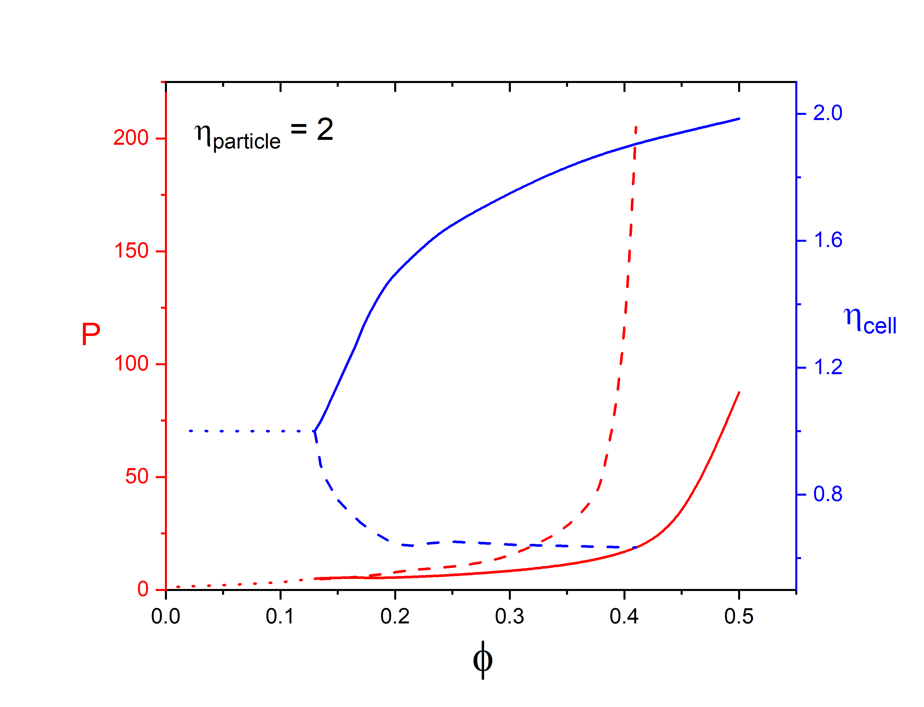
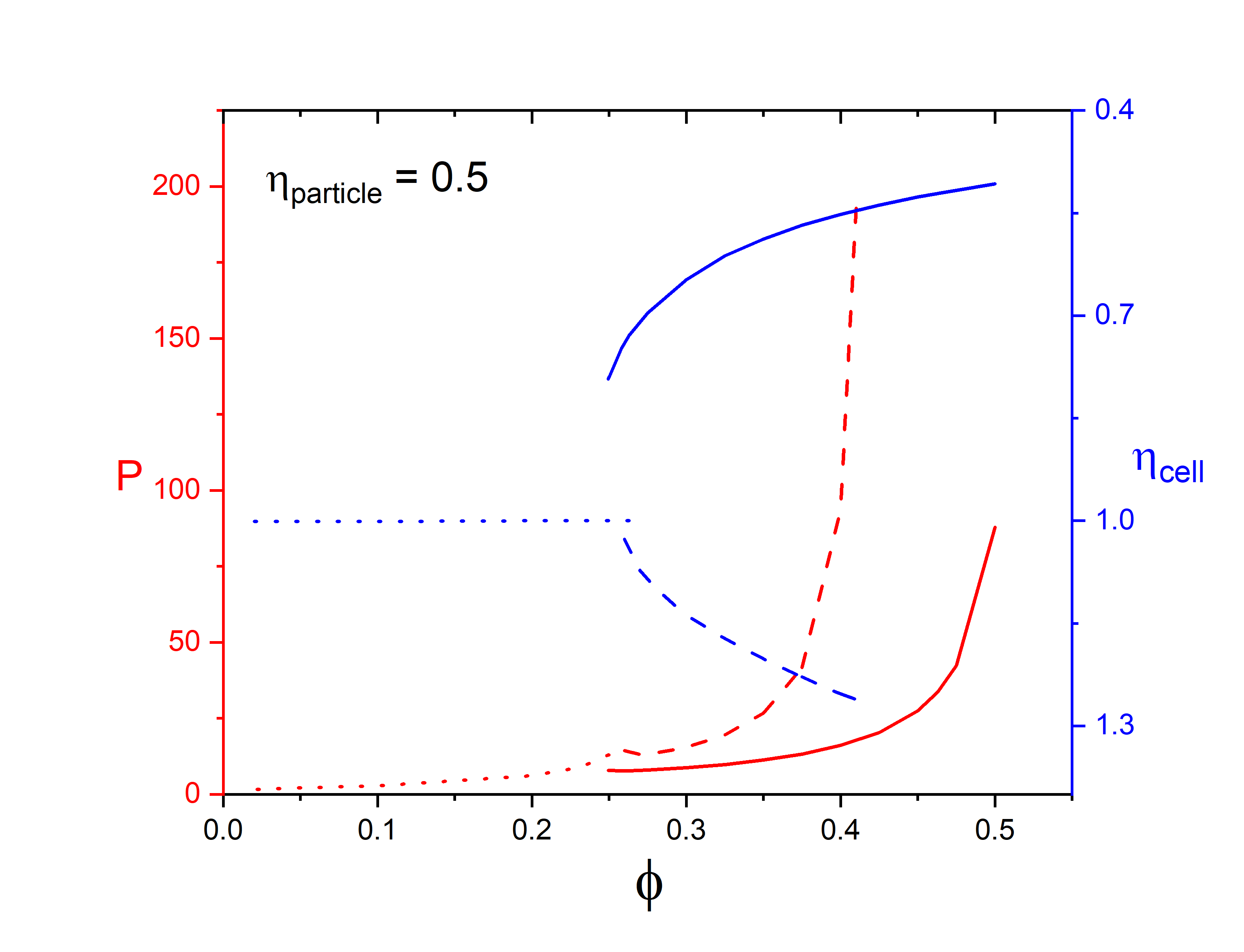
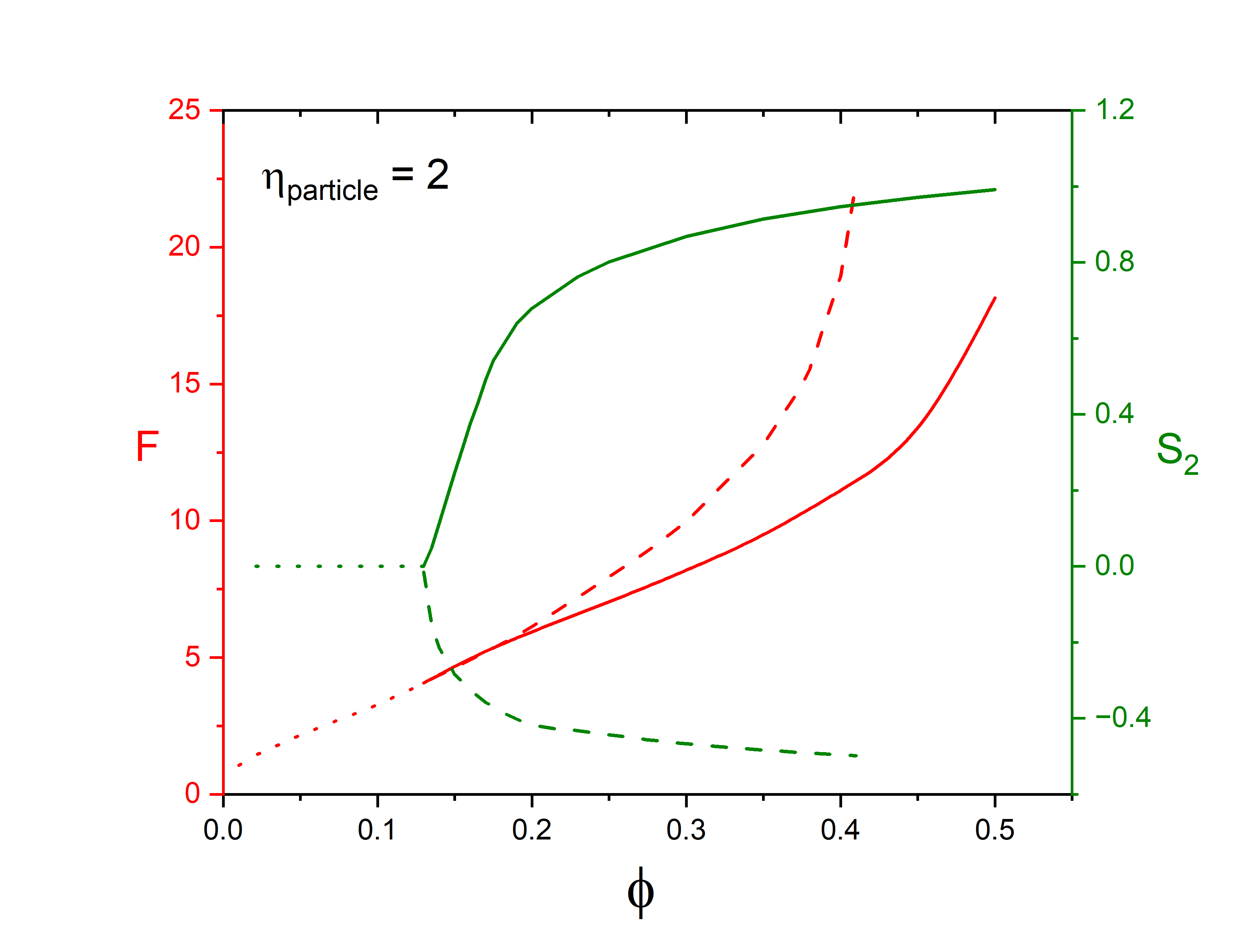
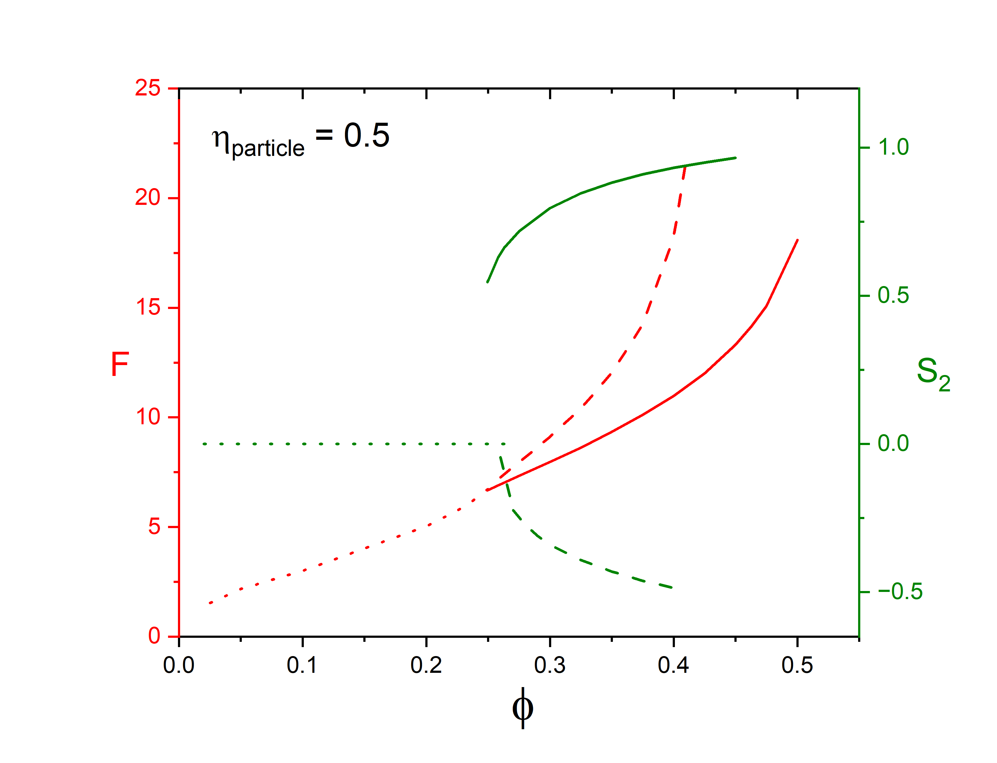
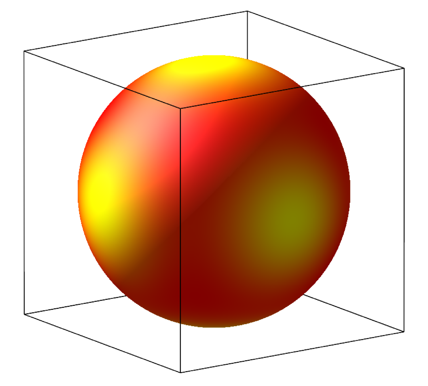
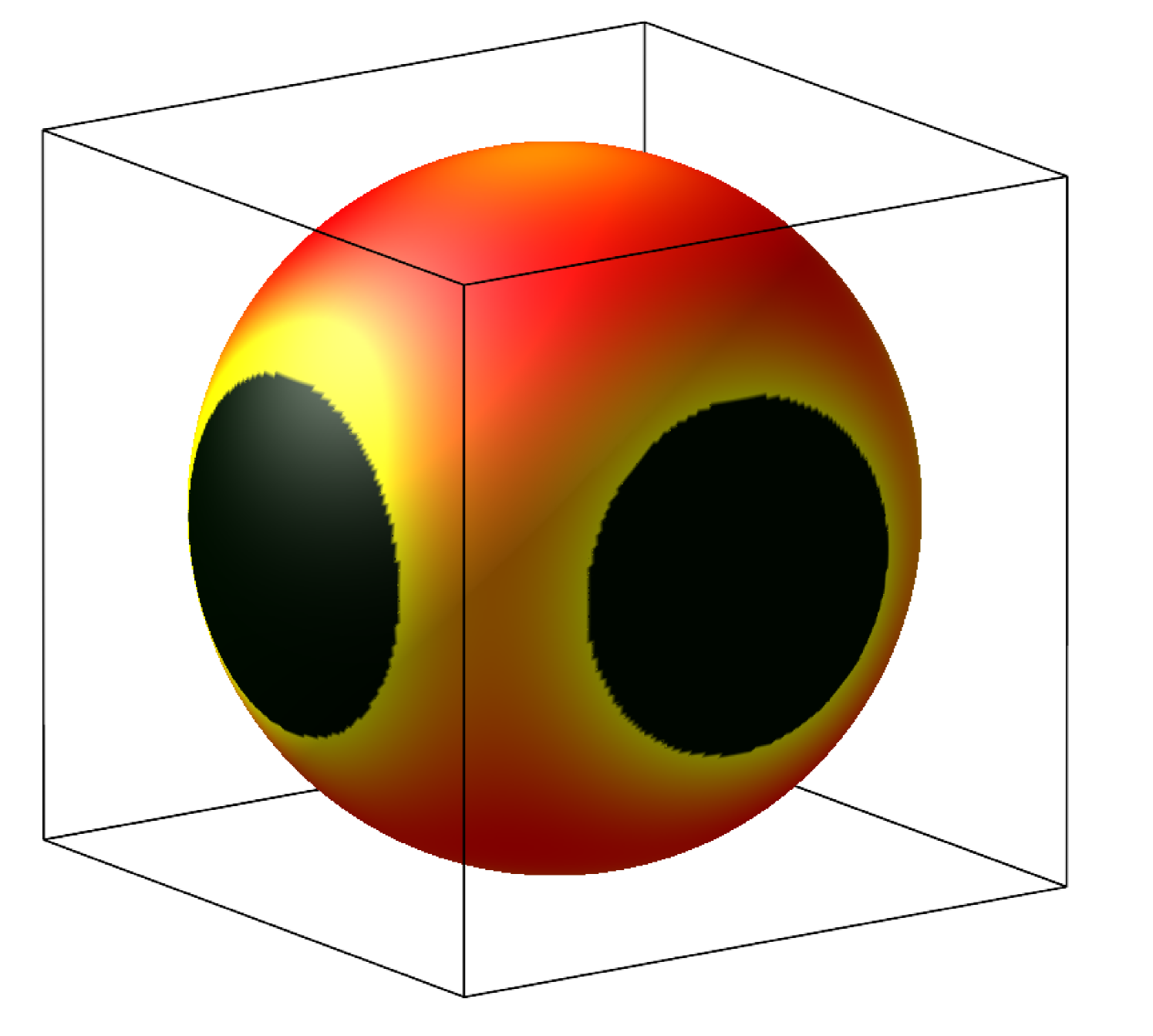
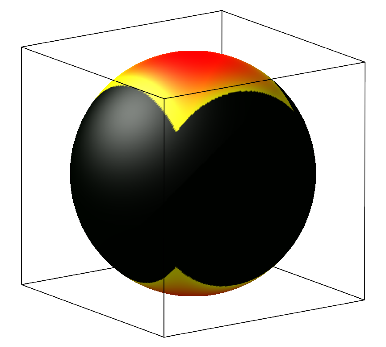
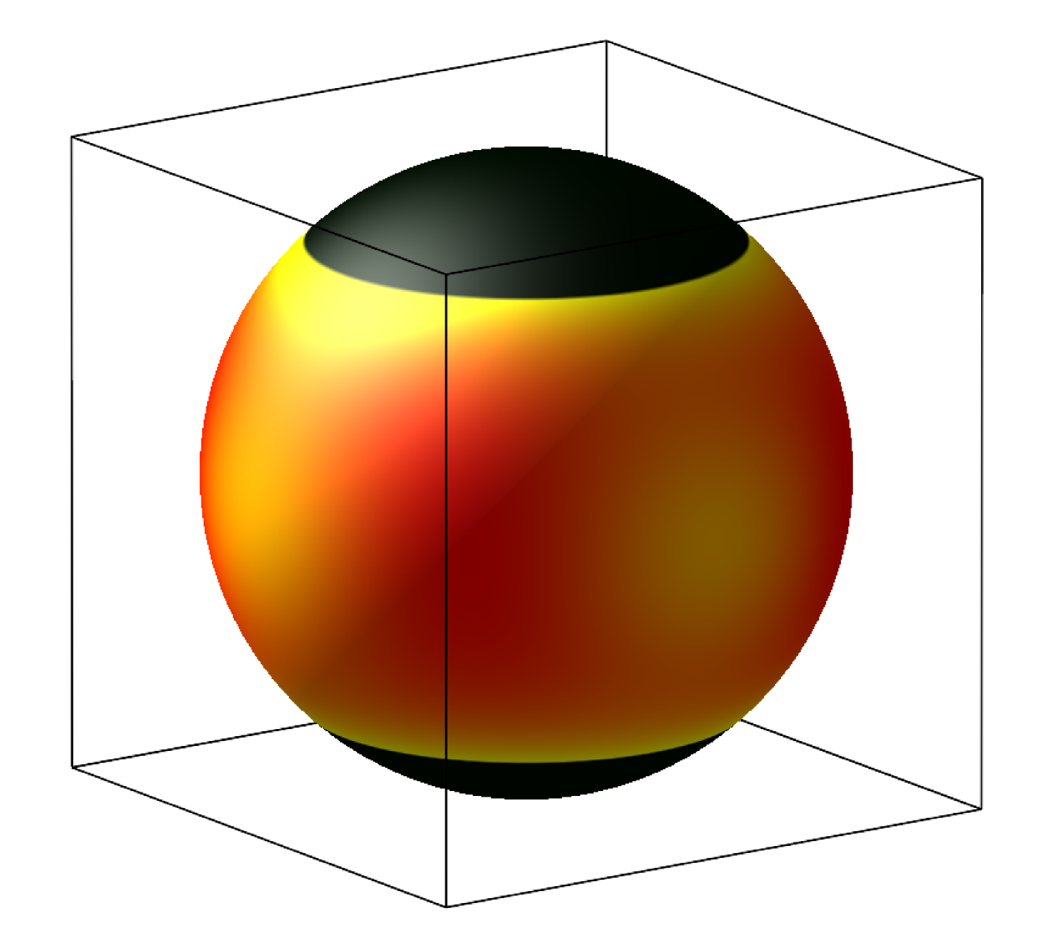
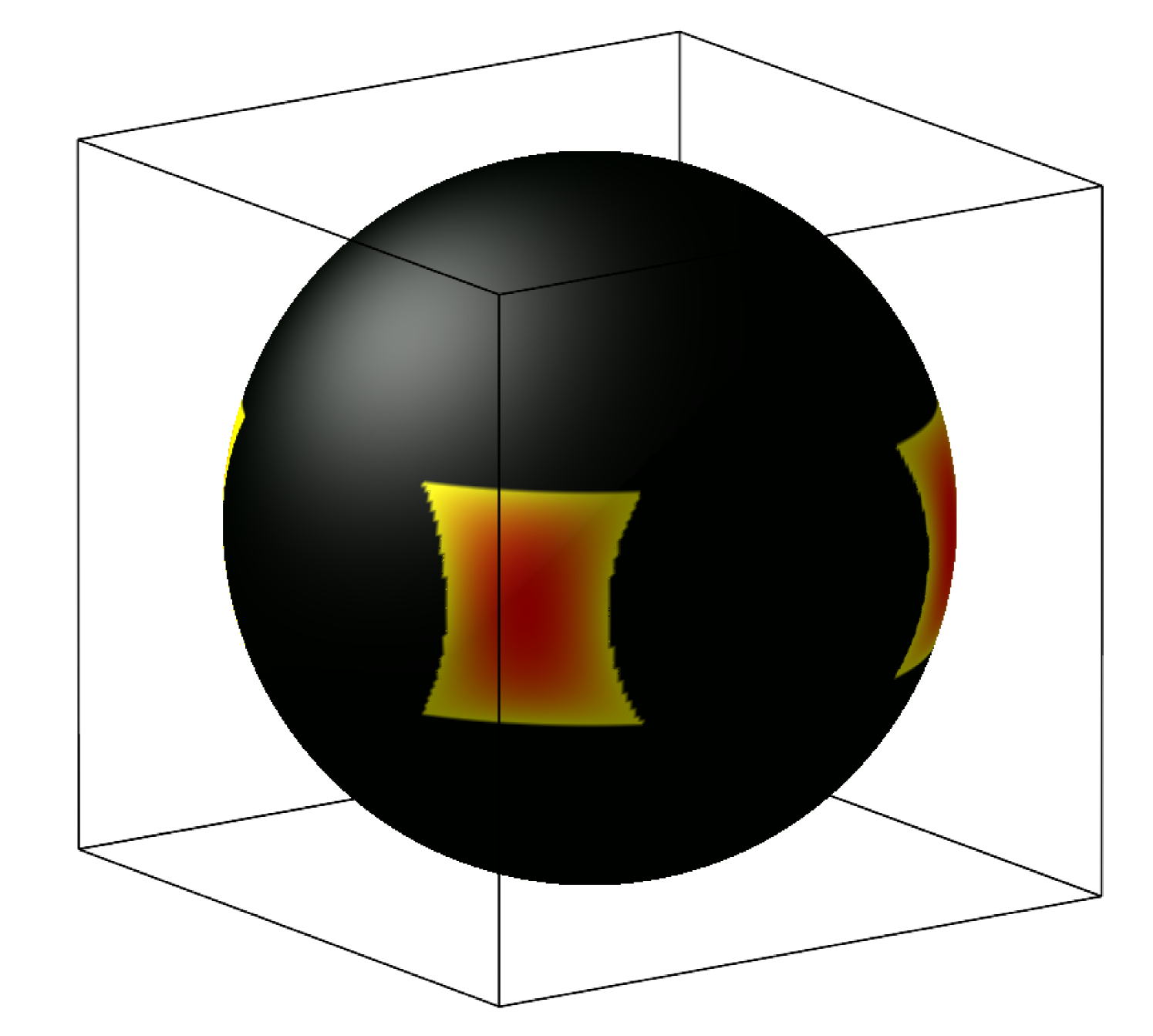
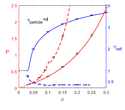
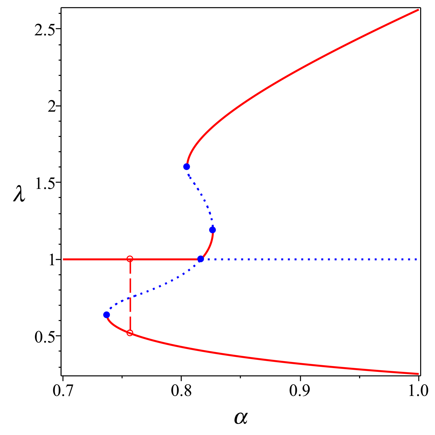
Figure 2 shows the results for two representative ellipsoids with aspect ratios and , respectively, as function of occupied volume fraction. Volume fraction was varied by changing particle volumes at fixed particle aspect ratio. Anisotropy at large volume fractions is apparent both in the cell shape, and in the orientational distribution function. Four scenarios have been observed: prolate or oblate particles in prolate or oblate cells. If the particle and cell shape are similar, then . If the particle and cell shapes are dissimilar, then .
For the prolate ellipsoid with , the system is dilute with , the whole orientation state space is accessible, the cubic cell with is the only minimiser of , and the orientational order parameter , the system is isotropic. At , the isotropic state loses its stability and two orientationally ordered solutions bifurcate from the isotropic branch. The prolate branch with has lower energy and pressure than those of the oblate branch with for .
For the oblate ellipsoid with , although the bifurcation is at , orientational order can be observed both below and above . In fact, there are two first order transitions from isotropic to both prolate nematic phase and oblate nematic phase at two different volume fractions slightly below . The prolate branch with possesses lower energy and pressure than those of the oblate branch with .
For sufficiently large volume fractions, certain orientations are disallowed by the shape of the cell, and the orientational distribution function has nontrivial compact support. This is indicated in Fig. 3(b-e), where representative equilibrium orientational probability density functions for a prolate ellipsoid with in equilibrium prolate (Figs. 3(b) and (c)) and oblate (Figs. 3(d) and (e)) cells are shown. One can readily see that the distribution function lacks axial symmetry, even in the very dilute limit where , as shown in Fig. 3(a). This is because an uniaxial ellipsoid has more free volume when it aligns along the diagonals of a rectangular cell compared to other orientations.
As the volume fraction is increased, a topological transition takes place: the connected accessible orientational space becomes disconnected forming a number of disconnected regions, where the orientation of the ellipsoid is locked in a small region, as can be observed in going from Figs. 3(b) to (c) and from (d) to (e). These topological changes also manifest themselves as kinks on the bifurcation diagrams as in Fig. 2 and Fig. 4, although the topological change on the prolate branch is not as apparent as the one on the oblate branch.
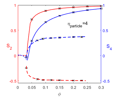
Since the orientational distribution function is known, in addition to , higher moments can be readily calculated. Here is the Legendre polynomial of degree . Although in the isotropic phase , interestingly, higher moments may exist as nonzero functions of the occupied volume fraction , as shown in Fig. 4(b). Given the edges and corners of the box, it is not surprising that the distribution function has higher moments which are nonzero at all volume fractions.
The free volume of an arbitrarily shaped particle in a rectangular cell can be calculated using a support function based approach, where the support function plays the role of the function in Eq. (22). We also remark that as long as the cell is convex, the free volume for a concave particle will be identical to that of its convex hull. Applying the support function approach to extend our model to particles with more complex shapes has already been initiated by one of us (JMT).
We realize that cell shapes other than rectangular boxes may allow more free volume to ellipsoidal particles; we expect that to every particle shape there corresponds an optimal cavity shape with the lowest free energy in equilibrium. The rectangular box is just our first attempt; an ellipsoidal cell is considered in Section 3.3.
3.2 Molecular dynamics
Molecular dynamics (MD) is a useful tool for studying properties of systems of interacting particles. MD simulations keep track of the motion of individual particles relying on classical mechanics. The results of MD simulations can be used to test the validity of statistical mechanical models. Here, we perform MD simulations of a hard rigid ellipsoidal particle moving in a rectangular cell, undergoing collisions with the cell walls. We imagine that this approximates the real physical situation where thermally excited molecules collide with nearest neighbors. As we show in this subsection, MD gives the same predictions for the equilibrium shape of the cell, for the average orientation of the ellipsoid, and for the pressure as our statistical mechanical model.
The dynamics consists of free flights and collisions with cell walls. When the particle does not undergo a collision, the position of its center of mass is updated as
| (26) |
However, the angular velocity of the particle changes in time even without external torque. The angular acceleration in an inertial reference frame is given by Euler’s equations for rigid body dynamics,
| (27) |
where is the tensor of inertia of the ellipsoid, given by
| (28) |
where is its uniformly distributed mass. We then update the angular velocity and the orientation of the particle as follows,
| (29) | |||||
| (30) |
where we use the default value of . If the updated configuration causes any part of the particle to leave the cell, we return to the previous step, and halve . The process is repeated until the new configuration of the particle is completely within the cell. When the time step size reaches a lower threshold (e.g., ), collision with the wall occurs.
We assume that both the particle and cell walls are frictionless, thus the impulses are along the normals to the surfaces in contact. In a collision, the conservation of linear momentum, angular momentum and kinetic energy, gives the postcollision center of mass velocity and angular velocity by ([12])
| (31) |
| (32) |
where and are precollision velocity and angular velocity, is the outward normal of the ellipsoid pointing towards the cell wall. The vector is a body-fixed vector joining the center of mass of the ellipsoid to the point of contact with the cell wall at the instant of collision,
| (33) |
and the positive scalar is the magnitude of the impulse transferred to the ellipsoid at the collision,
| (34) |
The pressure on each wall is the average impulse per area on the wall. If the pressure happens not to be isotropic, we then update the relevant length of the cell, denoted , according to
| (35) |
where and represent the averaged pressures on two square walls and four rectangular walls, respectively, and plays the role of compressibility. The updates for the other two dimensions are determined by maintaining constant volume and a uniaxial shape.
A very great deal of work has been done on simulations of systems of hard ellipsoids[13],[14],[15],[16]. Our system is different, however, due to the mean field aspect of our model, where only a single particle is present, enclosed by a cell representing the effects of the other particles. Confinement induced ordering of hard ellipsoids has also been studied between two hard walls [17] however our confinement is in 3D; furthermore the shape of the confining shape is adaptive.
The scalar order parameter is calculated according to where the average is over all instantaneous orientations of the symmetry axis of the ellipsoid between collisions. All simulation results were averaged over random initial conditions.
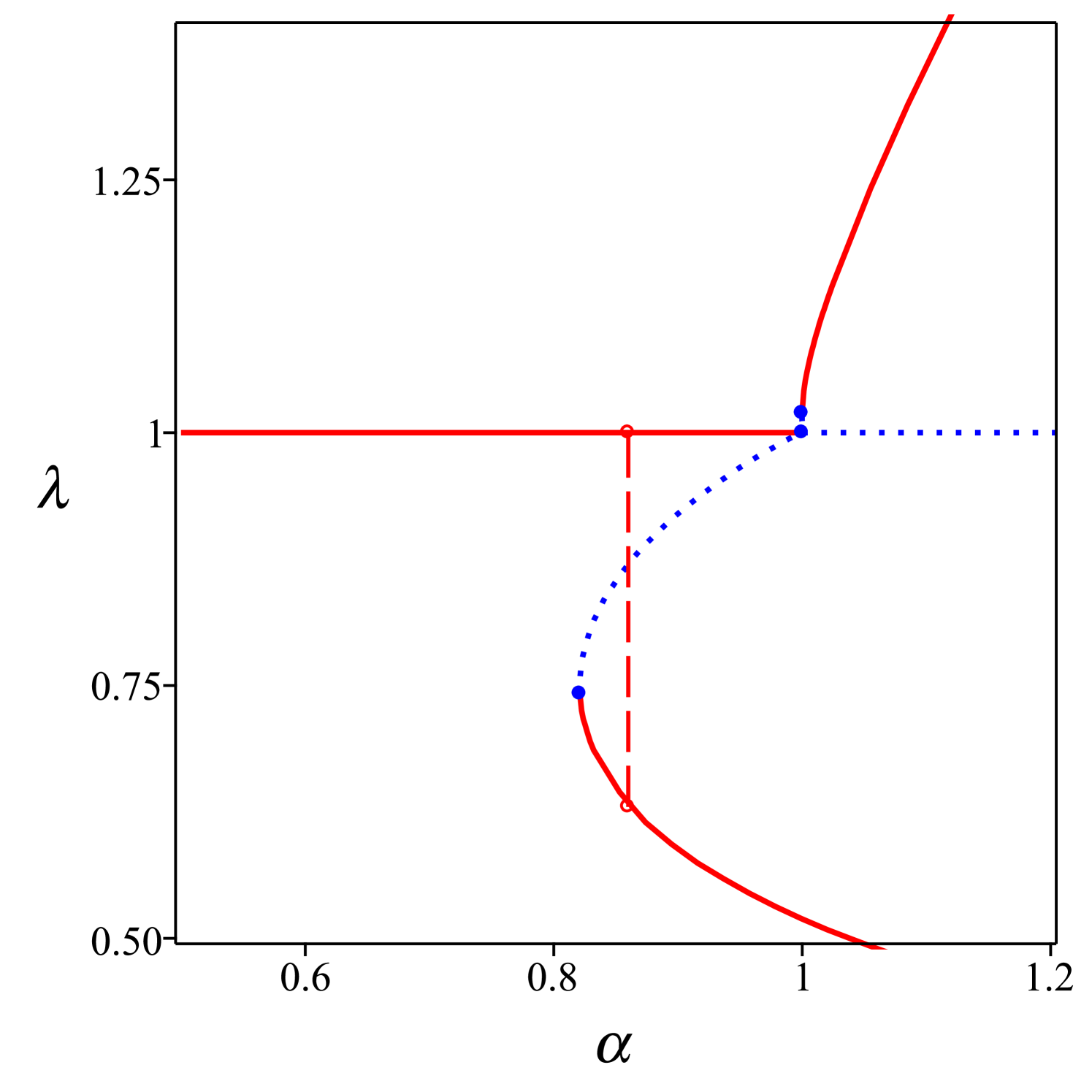
Figure 4 shows the agreement of the results of free volume calculation in Sect. 3.1 and MD simulations for an ellipsoid with aspect ratio . The transition from the isotropic phase to the prolate phase is continuous, whereas the transition from the isotropic phase to the oblate phase is discontinuous. This is different from the case of where both transitions are continuous.
3.3 Needle in an ellipsoidal cell
In this subsection, we consider a needle within an ellipsoidal cell. This geometry allows for an analytic free volume expression, and reveals a topology common to the case of very slender particles.
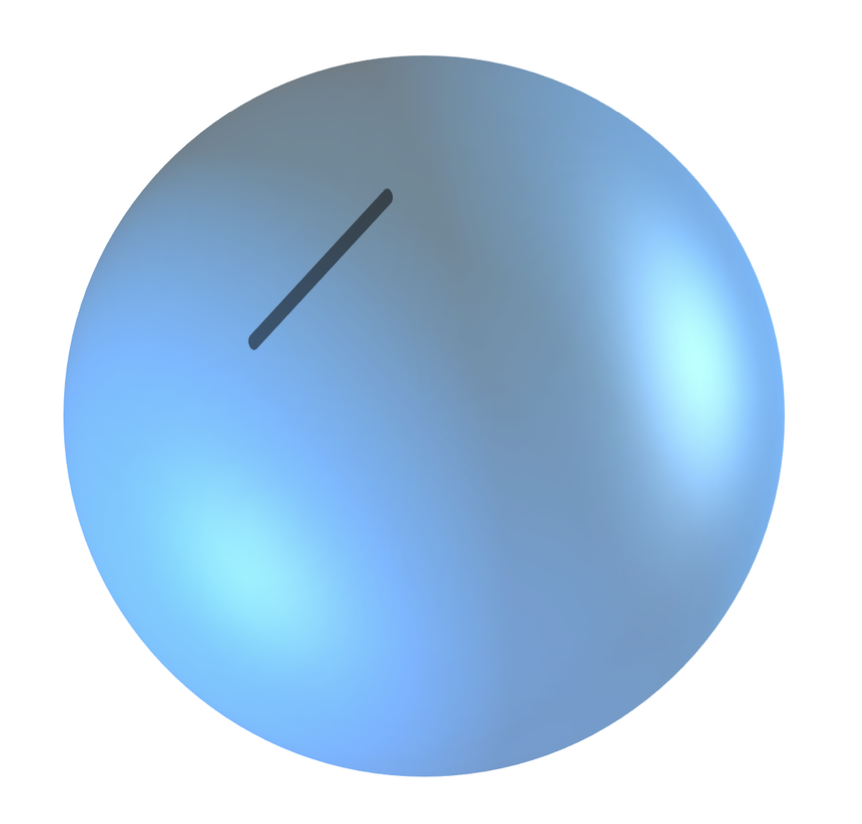
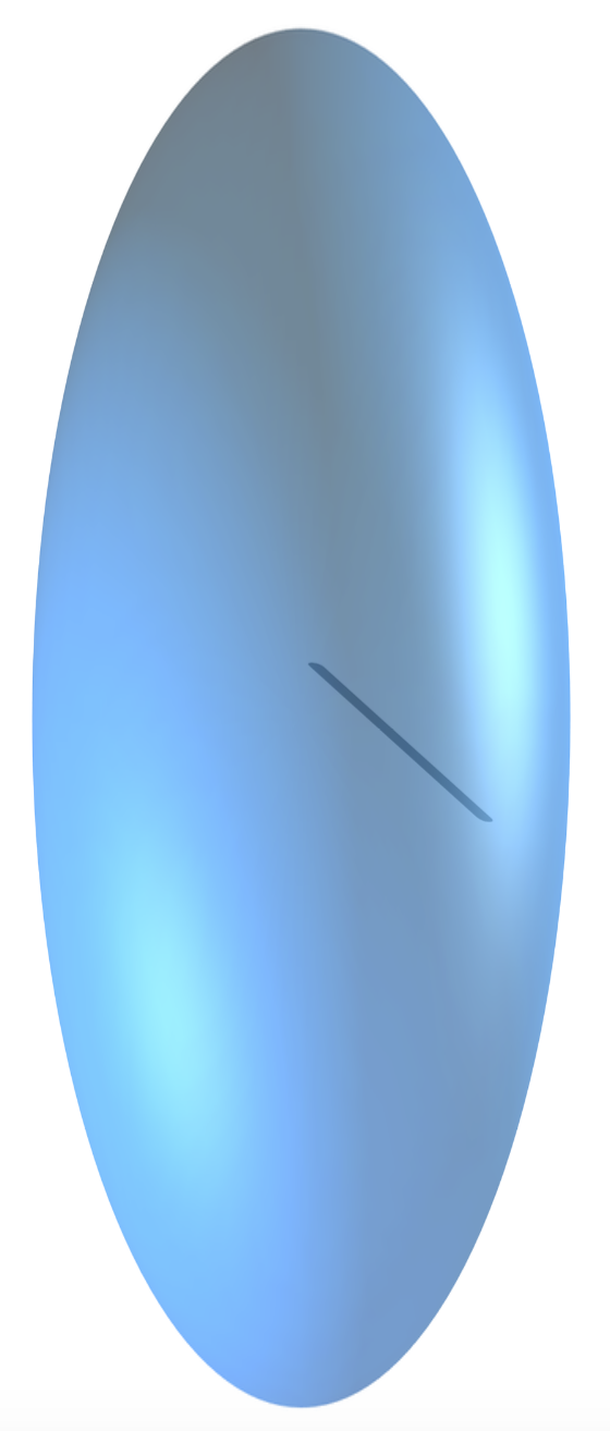
Consider to be a spherical cavity of radius enclosing a rigid rod of length (see Fig. 5(a)) and subject the sphere to a homogeneous, isochoric deformation with gradient , which, modulo a rotation, changes the sphere into the ellipsoid depicted in Fig. 5(b).
Now, the unit vector denotes the orientation of the rod, such that if the center of the rod is at the point , its ends occupy the points , respectively. We want to determine the volume of the free region accessible to within the ellipsoid , for a given orientation of the rod. Writing and , so that are the preimages of , and the preimage of , the region comprises all points such that
| (36) |
from which, since is invertible, we have that
| (37) |
and so
| (38) |
Geometrically, this set is the region comprised of two spheres of radius whose centers are apart, where
| (39) |
Since , the free volume is the same as the volume of , that is, twice the volume of a spherical frustum of radius and height ,
| (40) |
where is the volume of and we have set
| (41) |
It readily follows from (38) and (40) that
| (42) |
where is the left Cauchy-Green tensor, which in the frame of the principal directions of stretching is represented as
| (43) |
where , , and are the principal stretches subject to . Letting be the components of in the frame , they can be written as
| (44) |
for and . By use of (44) and (43) in (42) , we arrive at
| (45) |
For simplicity, we shall assume that has the uniaxial symmetry around , so that and reduces to
| (46) |
With this choice, the ellipsoid is prolate along if and oblate if .
For given , the domain of admissible values of is restricted by the second inequality in (41). A direct inspection shows that where
| (47) |
where
| (48) |
The free energy of the rod (in units ) is then given by
| (49) |
where the added constant has been gauged so as to ensure that . The integral in (49) can be expressed in terms of elementary functions, not given explicitly here in the interest of space. Plots of as function of are shown in Fig. 6 for several values of .
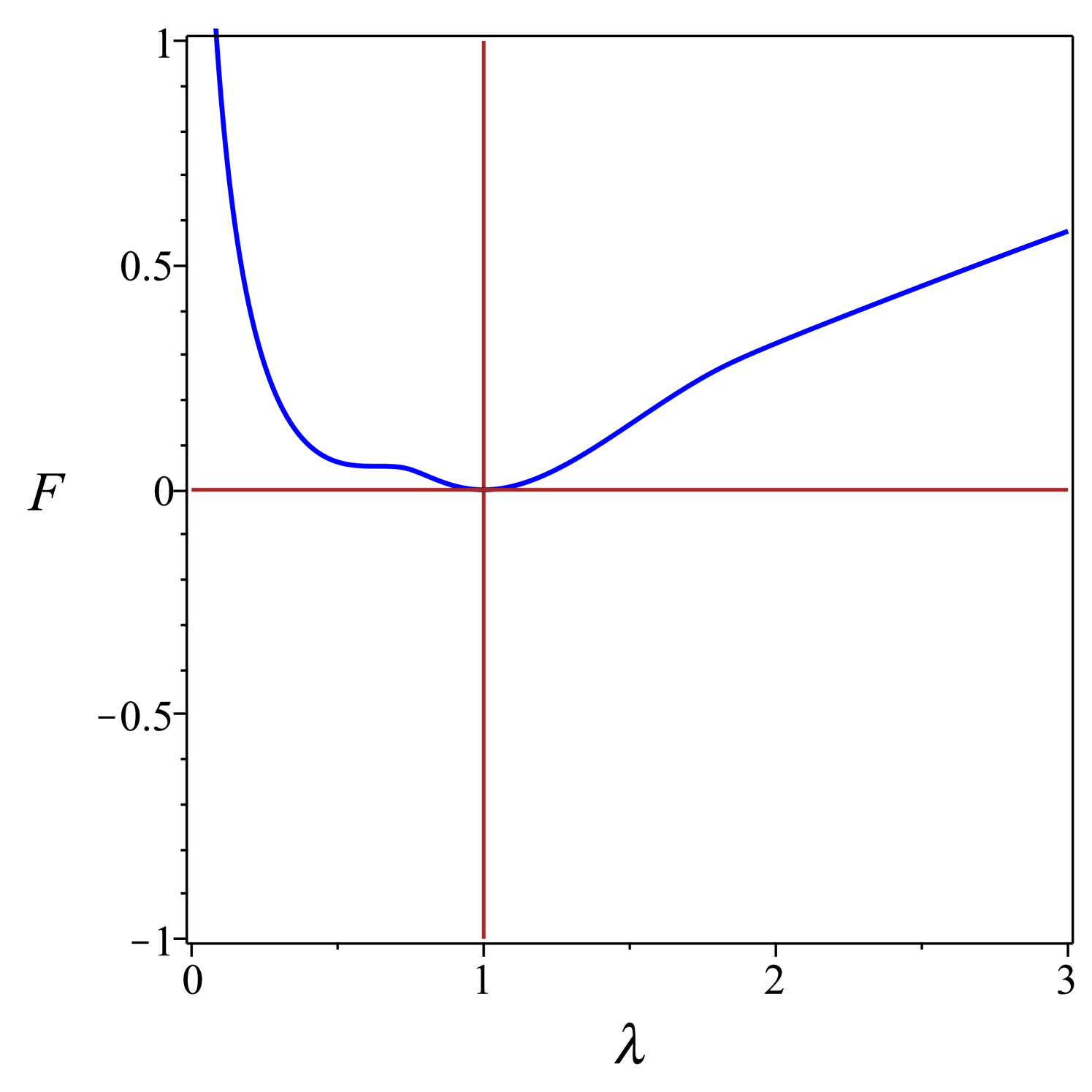
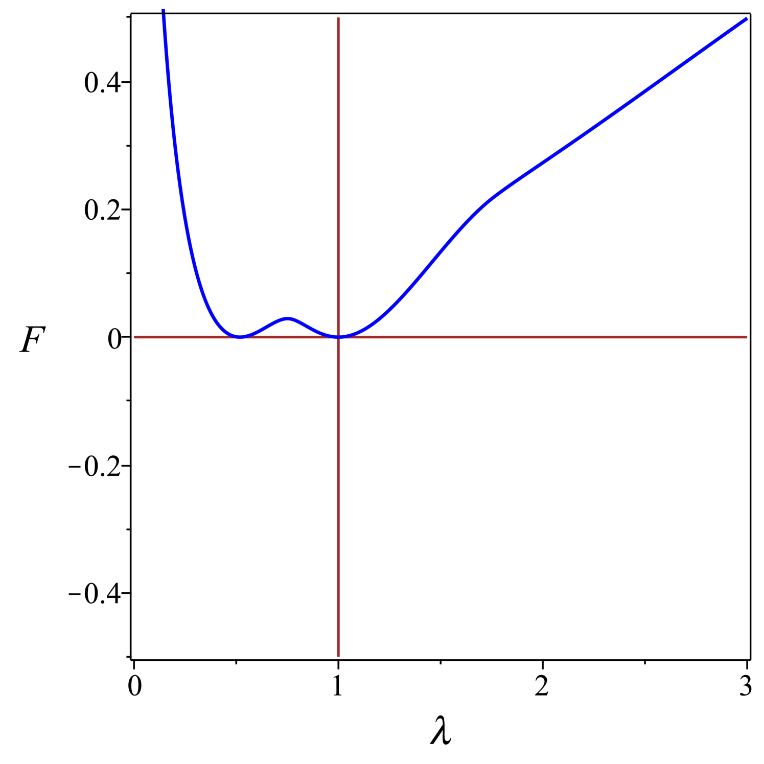
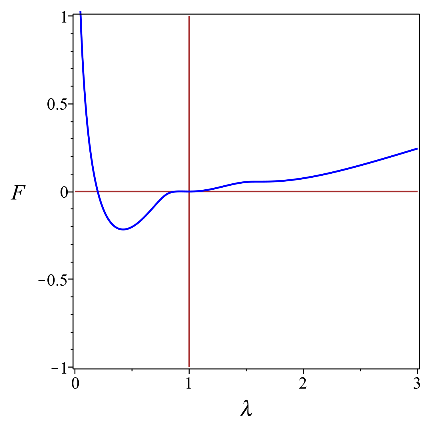
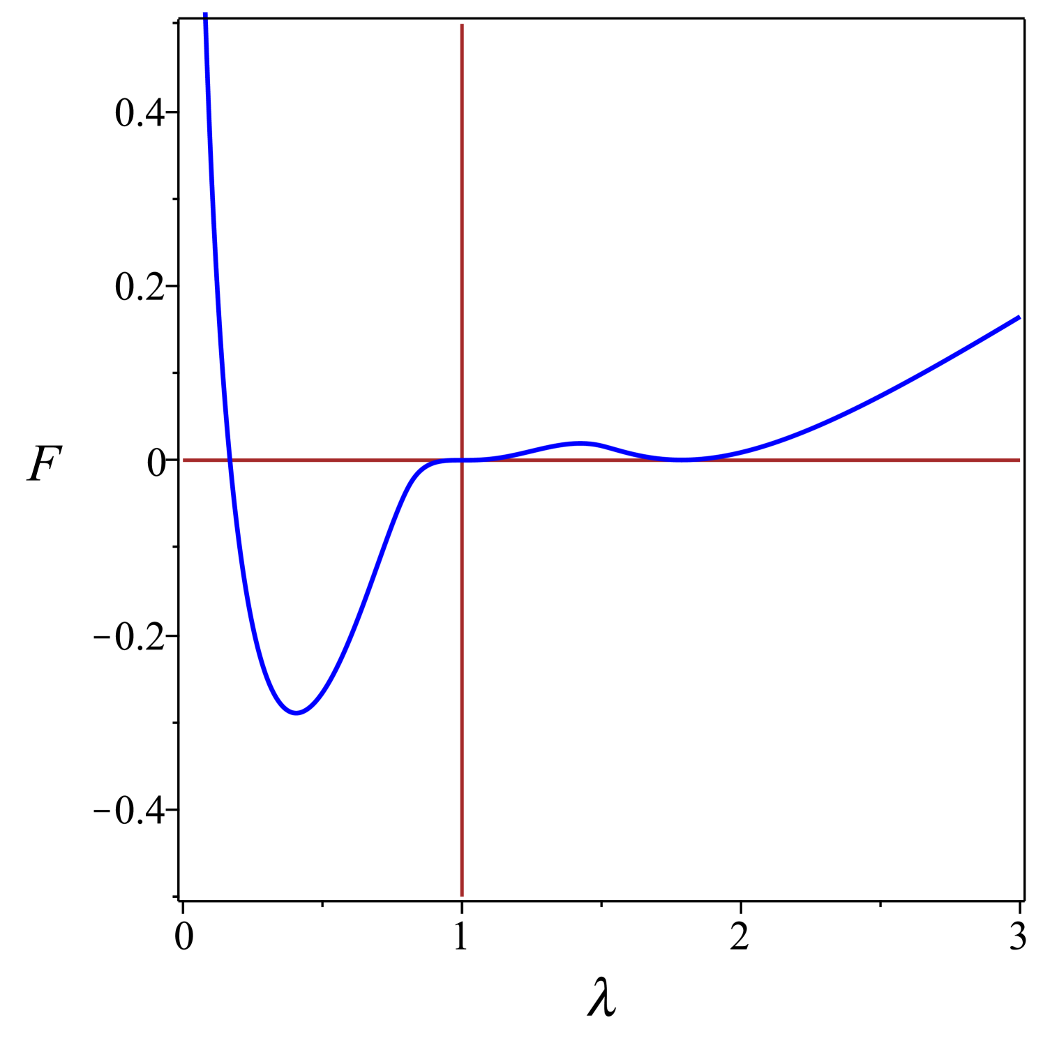
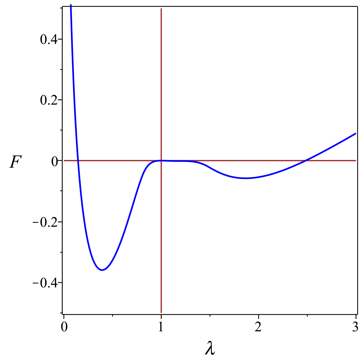
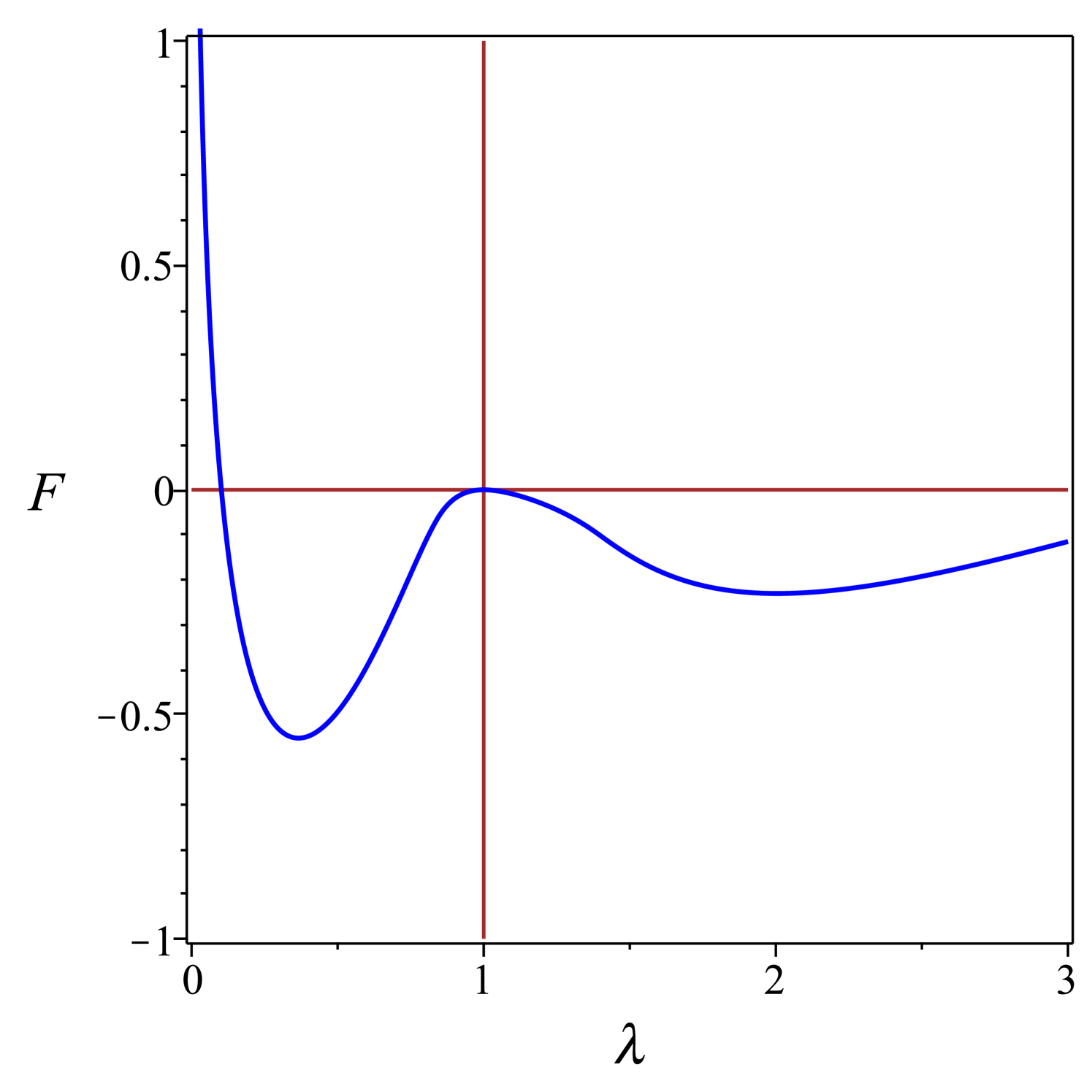
For , has a single critical point at , its absolute minimum representing the isotropic state where the spherical globule remains undeformed. For , a local minimum and a local maximum develop in the oblate branch (where ), while the isotropic state remains the absolute minimum, until reaches the transition value , where both the isotropic state and the oblate minimum have the same energy. A first-order transition takes place at , with the oblate minimum at . At , an inflection point develops on the prolate branch, from which a local maximum and a local minimum emanate, the former approaching the equilibrium isotropic state at . At , the isotropic state becomes unstable and two branches emanate from it, a local prolate minimum and a local oblate maximum: the former connects with the prolate maximum at , while the latter connects with the oblate minimum at . The locally stable prolate branch converges to as , whereas the globally stable oblate branch converges to as .
Figure 7 summarizes the above results, which are also compared with the bifurcation diagrams for a needle in a rectangular cell. We note that the topologies are mildly distinct. Whilst the oblate branch has a similar topology in each case, two unstable branches, one prolate and one oblate, bifurcate from the isotropic state at the critical value in the cuboidal case, with the former being a very small region that is difficult to see in the figure.
4 Work by shape change
Our mean field model gives some insights about the effects of shape change by individual molecules on their neighbors. A number of photomechanical materials consist of a nematic liquid crystal elastomer, containing a small fraction () of photoisomerizable azo dyes. These, in their ground state trans- configuration are elongated and in essence very similar to the liquid crystal molecules of the host. When illuminated, however, they undergo a trans-cis photoisomerization, and their shape changes from the elongated trans- form to the more compact – cis- form. Based on our model, we can estimate the free energy increase and stress on the host due to this shape change.
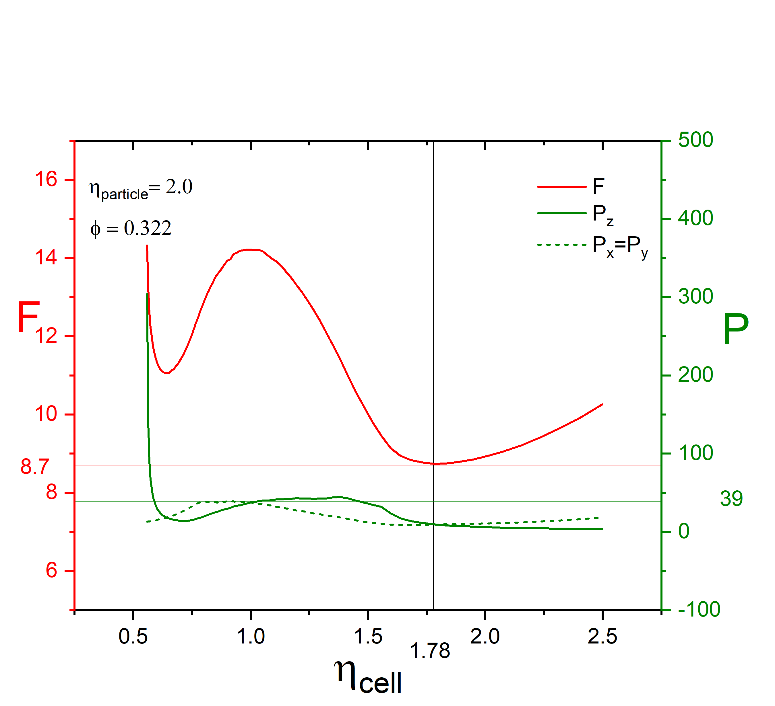
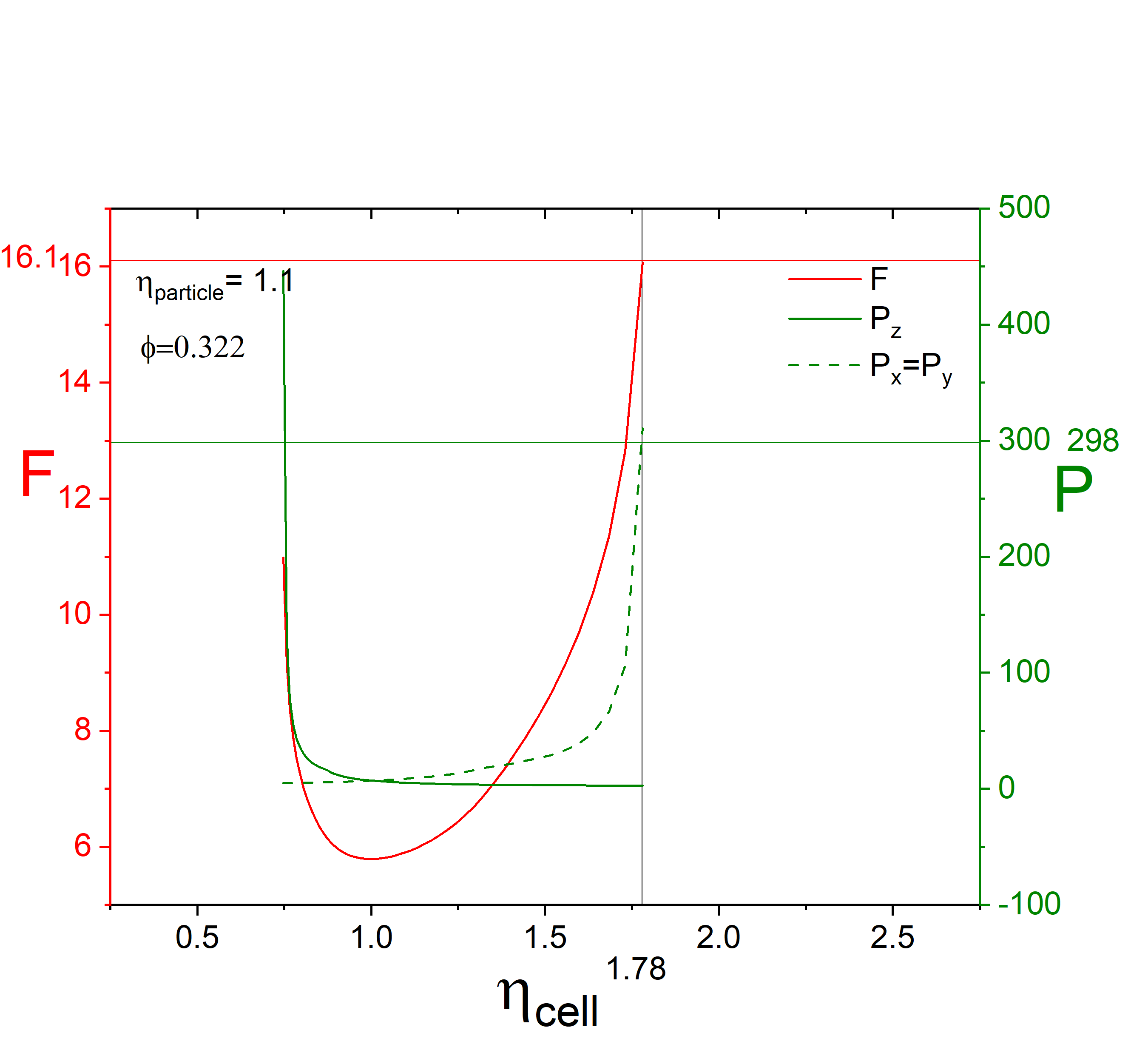
The aspect ratio of the trans- isomer is (roughly) known; we can also estimate the volume fraction. We know that in equilibrium the free energy is a minimum; so we minimize the free energy with respect to the cell aspect ratio. A possible starting configuration is shown in Fig. 8(a); the box shape is optimal for the given volume fraction and ellipsoid aspect ratio of ; the sample is in equilibrium and the pressure on the box is isotropic. The sample is then illuminated with UV light, and there is photoisomerization where the dye molecule changes its shape from the elongated trans- to the more spherical cis- shape. As the ellipsoid suddenly becomes more spherical, the system loses equilibrium, the free energy dramatically increases and the pressure becomes anisotropic as shown in Fig. 8(b). This is the initial free energy for the photowork, shown in Fig. 8(b), together with pressure, which is now strongly anisotropic.
If allowed, the cell shape then changes to aspect ratio close to to minimize the free energy for the new ellipsoid shape. The photomechanical work is carried out by the stress on the cell walls. The free energy corresponding to box aspect ratio is the final energy of the system after the photowork. The free energy difference between the initial and final states is the energy available for photowork.
In an isotropic medium, dissolved azo dyes behave like standard two-level systems, governed by a nearly constant potential energy difference between the tran- and cis- states. In a liquid crystal host, however, potential energy of each isomer111internal energy plus the work required to insert the isomer into the standard cell in the system would sensitively depend on the anisotropy of the cell. One would expect therefore that the temperature dependence of isomer populations in liquid crystals to significantly differ from that of a simple two-level system.
Energy for the photoexcitation comes from the absorbed photon; what is not used in increasing the free energy is released as heat. Matching the free energy increase to the absorbed photon energy may be a viable strategy to increase the efficiency of photomechanical materials.
5 Conclusion
In this work, we have considered a mean field model of indistinguishable particles with hard core steric interactions in a volume at temperature . The region is divided into identical cells, each with one particle in each cell. Each cell has a volume . At nonzero temperatures, the particles undergo collisions with the cell walls which approximate the effects of neighboring particles. In equilibrium, satisfying self-consistency, the cell adopts a shape which minimizes the free energy, and leads to an isotropic pressure tensor.
We have applied this mean field cell model to the case of hard uniaxial ellipsoids in rectangular and ellipsoidal cells.
At low occupied volume fractions, the shortest dimension of the cell is longer than the longest dimension of the particles. Hence all orientations of the particles are possible in the cells; here the particles are orientationally disordered, and the orientational order parameter - the second moment of the orientational distribution - is zero. As the occupied volume fraction increases, there is a critical volume fraction where the shortest dimension of the cell is equal to the longest dimension of the particles. Above this critical volume fraction, the orientational distribution function has compact support; there is a bifurcation and the system becomes orientationally ordered. One of the orientationally ordered solutions is prolate, while the other is oblate; the stability is determined by the shape of the cell. The results of mean-field theory are fully compatible with the the results of molecular dynamics simulations.
The above results give insights towards understanding the shape change exhibited by photomechanical materials. In such azo-dye doped liquid crystal elastomer materials, illumination causes photoisomerization of the dye. Due to the shape change, the system loses equilibrium, the free energy increases and anistoropic stress appears in the cell, which changes the shape of the cell and of the bulk host, and can do mechanical work. Energy for the work comes from the absorbed light. The model not only describes the mechanism whereby particle shape change results in local increased free energy and anisotropic internal stress, but allows quantitative estimates of these.
This paper has reported our first attempts to implement a simple mean field theory for rod-like hard particles. Work to extend and improve the model is clearly needed. Allowing the confined particles to respond to the anisotropic internal pressures acting on them seems promising; as does consideration of cell and particle shapes more general than those considered here. Efforts in these directions are under way.
Acknowledgements
P.P-M. acknowledges support from the Office of Naval Research through the MURI on Photomechanical Material Systems (ONR N00014-18-1-2624).
References
- [1] Camacho-Lopez M., Finkelmann, H.,Palffy-Muhoray, P. and Shelley, M. Fast liquid crystal elastomer swims into the dark, Nature Materials, 3, 307-310 (2004)
- [2] White T.J., Broer, D.J. Programmable and adaptive mechanics with liquid crystal polymer networks and elastomers, Nature Materials, 14, 1087-1098 (2015)
- [3] M. G. Kuzyk and N.J. Dawson, Photomechanical materials and applications: a tutorial, Advances in Optics and Photonics 12, 847 (2020)
- [4] Guo, T., Svanidze,A., Zheng, X. Palffy-Muhoray, P. Regimes in the Response of Photomechanical Materials, Appl. Sci. 12, 7723, 2022
- [5] Onsager L. The effects of shape on the interaction of colloidal particles. Annals of the New York Academy of Sciences. 1949 May;51(4):627-59.
- [6] Lennard-Jones JE, Devonshire AF. Critical phenomena in gases-I. Proceedings of the Royal Society of London. Series A-Mathematical and Physical Sciences. 1937 Nov 5;163(912):53-70.
- [7] Kincaid JF, Eyring H, Stearn AE. The Theory of Absolute Reaction Rates and its Application to Viscosity and Diffusion in the Liquid State. Chemical Reviews. 1941 Apr;28(2):301-65.
- [8] Kirkwood JG. Critique of the free volume theory of the liquid state. The Journal of Chemical Physics. 1950 Mar;18(3):380-2.
- [9] A.L. Kuzemsky, Variational Principle of Bogoliubov and Generalized Mean Fields in Many-Particle Interacting Systems, Int.J. Mod. Phys. B 29, (2015)
- [10] Palffy-Muhoray, P., The single particle potential in mean field theory, Am. J. Phys. 70, 422-437 (2002)
- [11] Spencer, A.J.M., 2004. Continuum mechanics. Courier Corporation.
- [12] Palffy-Muhoray, P., Virga, E. G., Wilkinson, M., Zheng, X., On a paradox in the impact dynamics of smooth rigid bodies. Mathematics and Mechanics of Solids, 24(3), 573-597 (2019).
- [13] D. Frenkel and B. M. Mulder, Mol. Phys. 55, 1171 (1985)
- [14] J.W.Perram, M.S.Wertheim, J.L. Lebowitz ,and G.O.Williams,Chem. Phys.Lett.105,277(1984).
- [15] G. Bautista-Carbajal, A. Moncho-Jorda and G. Odriozola, Further details on the phase diagram of hard ellipsoids o frevolution, J. Chem. Phys. 138, 064501 (2013)
- [16] B.J.Berne and P.Pechukas,J.Chem.Phys.56,4213(1972)
- [17] H. Miao and H. Ma, Confinement Induced Ordering in Fluid of Hard Ellipsoids, Chin. J. Chem. Phys. 29, 212 (2016)