A coupled-channel perspective analysis on bottom-strange molecular pentaquarks

Qing-Fu Song 242201003@csu.edu.cn School of Physics, Central South University, Changsha 410083, China Qi-Fang Lü lvqifang@hunnu.edu.cn Department of Physics, Hunan Normal University, Changsha 410081, China Key Laboratory of Low-Dimensional Quantum Structures and Quantum Control of Ministry of Education, Changsha 410081, China Key Laboratory for Matter Microstructure and Function of Hunan Province, Hunan Normal University, Changsha 410081, China Xiaonu Xiong xnxiong@csu.edu.cn School of Physics, Central South University, Changsha 410083, China

Abstract

At present work, we systematically study various bottom-strange molecular pentaquarks to search for possible bound states and resonances by adopting one-boson-exchange model within complex scaling method. According to our calculations, we predict several bound and resonant states for bottom baryon $Y_{b}(\Lambda_{b},\Sigma_{b})\bar{K}^{(*)}$ and $Y_{b}K^{(*)}$ systems. In particular, a bound state in the $I(J^{P})=1/2(1/2^{-})$ $\Sigma_{b}\bar{K}/\Lambda_{b}\bar{K}^{*}/\Sigma_{b}\bar{K}^{*}$ system may correspond to the particle $\Xi_{b}(6227)$ . Meanwhile, the predicted bound state with $6303\sim 6269~{}\rm{MeV}$ in the $I(J^{P})=1/2(1/2^{-})\Sigma_{b}K/\Lambda_{b}K^{*}/\Sigma_{b}K^{*}$ system is flavor exotic and does not appear in the spectroscopy of conventional baryons, which provides a practical way to clarify the nature of particle $\Xi_{b}(6227)$ . We highly hope that our proposals can offer helpful information for the future experimental searches.

molecular states, coupled-channel analysis, complex scaling method

pacs:

12.39.Pn, 13.75.Lb, 14.40.Rt

I introduction

After the discovery of the $X(3872)$ on the Belle experiment Belle:2003nnu in 2003, a large amount of data has been accumulated in the past two decades in high energy collision experiments. In the mean while, a series of new phenomenology studies related to the $XYZ$ and $P_{c}/T_{cc}$ states have been reported Liu:2019zoy ; Liu:2015fea . A detialed investigation of those exotic hadron states provides new insights for decoding their internal structures, which may deepen our understanding of the nonperturbative properties of quantum chromodynamics (QCD). Since many new particles locate near the hadron-hadron thresholds, these states could be naturally interpreted as candidates of molecular states Chen:2022asf ; Dong:2017gaw ; Guo:2017jvc ; Karliner:2017qhf ; Zou:2021sha ; Mai:2022eur ; Zou:2013af . It is highly desirable to identify those molecules states out of lots of candidates and predict more ones for experimental searches, which will motivate the experimental search of such molecular states.

In 2021, the LHCb collaboration reported two resonances, namely $X_{0}(2900)$ and $X_{1}(2900)$ in $D^{-}K^{+}$ invariant mass spectrum by analyzing the decay amplitude of the $B^{+}\to D^{+}D^{-}K^{+}$ decay channel LHCb:2020pxc ; LHCb:2020bls . Since these two states are located near the $\bar{D}^{*}K^{*}$ and $\bar{D}_{1}^{*}K^{*}$ threshold, they are regarded as hadronic molecules candidates Chen:2020aos ; He:2020btl ; Burns:2020epm ; Agaev:2020nrc ; Xiao:2020ltm ; Kong:2021ohg ; Ke:2022ocs . Recently, in the analysis of $D_{s}^{+}\pi^{+}$ and $D_{s}^{+}\pi^{-}$ invariant mass spectrum, the LHCb collaboration has observed two new peaks $T_{c\bar{s}0}^{0}(2900)$ and $T_{c\bar{s}0}^{++}(2900)$ , whose masses and widths are $M(T_{c\bar{s}0}^{0})=2892\pm 14\pm 15$ $\rm MeV$ , $\Gamma=119\pm 26\pm 12$ $\rm MeV$ and $M(T_{c\bar{s}0}^{++})=2921\pm 17\pm 19$ $\rm MeV$ , $\Gamma=137\pm 32\pm 14$ $\rm MeV$ LHCb:2022sfr ; LHCb:2022lzp , respectively. Given their near-threshold behaviors and quantum numbers, these two $T_{c\bar{s}0}^{0(++)}$ states are proposed as isovector $D^{*}K^{*}$ molecules with $J^{P}=0^{+}$ Agaev:2022eyk ; Wang:2023hpp ; An:2022vtg .

Until now, most molecular candidates were observed in the charm sector, while the experimental observations in the bottom sector are still scarce. In 2006, the DØ Collaboration announced a narrow structure, referred to as the $X(5568)$ in $B_{s}^{0}\pi^{\pm}$ channel D0:2016mwd . Then, the LHCb collaboration investigated the $B_{s}^{0}\pi^{\pm}$ invariant mass spectrum, but no significant signal is found LHCb:2016dxl . Later, the ATLAS, CDF, and CMS collaborations ATLAS:2018udc ; CDF:2017dwr ; CMS:2017hfy released similar results. Meanwhile, the $X(5568)$ has been theoretically discussed in previous works Chen:2016ypj ; Xiao:2016mho ; Agaev:2016urs , and can not be assigned as an isovector $BK$ molecular state. In 2021, the LHCb collaboration reported two states in $B^{\pm}K^{\pm}$ mass spectrum, which are named as $B_{sJ}(6063)$ and $B_{sJ}(6114)$ . If the missing photo from the $B^{*\pm}\to B^{\pm}\gamma$ was taken into consideration, the masses and widths were measured to be $B_{sJ}(6109):M=6108.8\pm 1.1\pm 0.7\rm MeV\text{ and }\Gamma=22\pm 5\pm 4\rm MeV$ and $B_{sJ}(6158):M=6158\pm 4\pm 5\rm MeV\text{ and }\Gamma=72\pm 18\pm 25\rm MeV$ LHCb:2020pet , respectively. In theory, the $B_{sJ}(6158)$ was widely investigated in the literature Kong:2021ohg . Some of the existing works suggested that $B_{sJ}(6158)$ can be interpreted as a $\bar{B}K^{*}$ molecular state with $I(J^{PC})=0(1^{+})$ . Also, several works showed that the existence of $\bar{B}^{(*)}K^{(*)}(B^{(*)}\bar{K}^{(*)})$ molecular states are allowed Kolomeitsev:2003ac ; Guo:2006fu ; Guo:2006rp ; Sun:2018zqs .

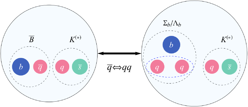
It can be seen that numerous exotic hadronic molecular states containing heavy quarks have been observed experimentally. The heavy quark symmetry is supposed to have been proven to play a significant role in predicting undiscovered states and understanding their production mechanisms, which intrigues several theoretical studies of it Asanuma:2023atv ; Tanaka:2024siw ; Wang:2023eng ; Sakai:2023syt . In a previous work, the author investigated open charm molecular counterpart of the newly $T_{c\bar{s}}^{a0(++)}$ composed of $Y_{c}(\Lambda_{c},\Sigma_{c})$ and strange meson $K^{(*)}$ interactions by adopting one boson exchange model. From their estimations, there can exist some bound states corresponding to the new observation $T_{c\bar{s}}^{a0(++)}$ Chen:2022svh . According to the heavy quark symmetry, on the bottom sector, the light diquark in the heavy baryons $\Sigma_{b}/\Lambda_{b}$ has the same color structure as $\bar{q}$ , as shown in Figure 1. If $B_{sJ}(6158)$ can be explained as a $\bar{B}K^{*}$ molecular state with $I(J^{PC})=0(1^{+})$ , there should also exist possible isoscalar $\bar{B}^{(*)}K^{(*)}$ molecular state. Under the circumstances, it is natural to conjecture whether there could exist possible open bottom molecular pentaquarks. Moreover, it is worth mentioning that, in 2018, the LHCb reported a peak in both $\Lambda_{b}^{0}K^{-}$ and $\Xi_{b}^{0}\pi^{-}$ invariant mass spectra named $\Xi_{b}(6227)$ LHCb:2018vuc . However, until now, whether the $\Xi_{b}(6227)$ should be accommodated into traditional baryon $\lambda-$ mode $P-$ wave $\Xi_{b}^{\prime}$ with $J^{P}=3/2^{-}$ and $5/2^{-}$ Chen:2018orb ; He:2021xrh ; Wang:2018fjm ; Cui:2019dzj or molecular state pure $\Sigma_{b}\bar{K}$ with $J^{P}=1/2^{-}$ is still on discussion Huang:2018bed ; Zhu:2020lza ; Mutuk:2024elj . Thus, it is urgent and necessary to explore the possibility of $\Xi_{b}(6227)$ being a molecular states and predict more bottom-strange molecular pentaquark candidates for future experiments.

Refer to caption — Figure 1: A sketch of heavy superflavor symmetry between $\Sigma_{b}(\Lambda_{b})K^{(*)}$ pentaquarks and $\bar{B}K^{(*)}$ tetraquarks. $q$ stands for the light quarks ( $u$ or $d$ ).

Recently, we systematically study the hidden bottom molecular tetraquark with complex scaling method by adopting one-boson-exchange(OBE) model Song:2024ngu , at present work, utilizing the same formulism, we systematically study various bottom-strange molecular pentaquarks to search for possible bound states and resonances by adopting within complex scaling method Aguilar:1971ve ; Balslev:1971vb ; Moiseyev:1998gjp ; Ho:1983lwa ; He:2021xrh and Gaussian expansion method Hiyama:2003cu ; Hiyama:2018ivm . For bottom baryon $Y_{b}(\Lambda_{b},\Sigma_{b})$ and anti-strange meson $\bar{K}^{(*)}$ interactions, our calculations demonstrate that some bound and resonant states are reveled. For instance, in the $I(J^{P})=1/2(1/2^{-})$ $\Sigma_{b}\bar{K}/\Lambda_{b}\bar{K}^{*}/\Sigma_{b}\bar{K}^{*}$ system, we obtain a bound state below $\Sigma_{b}\bar{K}$ threshold that can be regarded as the particle $\Xi_{b}(6227)$ . Meanwhile, we extend our study to $Y_{b}K^{(*)}$ systems, and find two flavor exotic bound states, which can be searched in future experiments.

The rest of this paper is organized as follows. We briefly introduce the formalism of effective interactions and complex scaling method in Sec. II. In Sec. III, we present the numerical results and discussions for the $Y_{b}$ $K^{(*)}$ and $Y_{b}$ $\bar{K}^{(*)}$ systems. Finally, we summarize in Sec. 4.

II Formalism of effective interaction and complex scaling method

II.1 The effective interactions

In this work, we adopt the one-boson-exchange model to describe the interaction between the hadrons and analyze the formation mechanisms of molecular states. The chrial symmetric interacting Lagrangian which corresponds to the coupling between a bottom baryon and a light mesons, can be constructed as Liu:2011xc

$\displaystyle\mathcal{L}_{\mathcal{B}_{\bar{3}}}$	$\displaystyle=$	$\displaystyle l_{B}\langle\bar{\mathcal{B}}_{\bar{3}}\sigma\mathcal{B}_{\bar{3}}\rangle+i\beta_{B}\langle\bar{\mathcal{B}}_{\bar{3}}v^{\mu}(\mathcal{V}_{\mu}-\rho_{\mu})\mathcal{B}_{\bar{3}}\rangle,$	(1)
$\displaystyle\mathcal{L}_{\mathcal{B}_{6}}$	$\displaystyle=$	$\displaystyle l_{S}\langle\bar{\mathcal{S}}_{\mu}\sigma\mathcal{S}^{\mu}\rangle-\frac{3}{2}g_{1}\varepsilon^{\mu\nu\lambda\kappa}v_{\kappa}\langle\bar{\mathcal{S}}_{\mu}A_{\nu}\mathcal{S}_{\lambda}\rangle$	(2)
	$\displaystyle+$	$\displaystyle i\beta_{S}\langle\bar{\mathcal{S}}_{\mu}v_{\alpha}\left(\mathcal{V}_{ab}^{\alpha}-\rho_{ab}^{\alpha}\right)\mathcal{S}^{\mu}\rangle+\lambda_{S}\langle\bar{\mathcal{S}}_{\mu}F^{\mu\nu}(\rho)\mathcal{S}_{\nu}\rangle,~{}$	(2)
$\displaystyle\mathcal{L}_{\mathcal{B}_{\bar{3}}\mathcal{B}_{6}}$	$\displaystyle=$	$\displaystyle ig_{4}\langle\bar{\mathcal{S}^{\mu}}A_{\mu}\mathcal{B}_{\bar{3}}\rangle+i\lambda_{I}\varepsilon^{\mu\nu\lambda\kappa}v_{\mu}\langle\bar{\mathcal{S}}_{\nu}F_{\lambda\kappa}\mathcal{B}_{\bar{3}}\rangle+h.c..$	(3)

The axial current $A_{\mu}$ , vector current $\mathcal{V}_{\mu}$ , and the vector meson field strength tensor $F^{\mu\nu}(\rho)$ are defined by

$\displaystyle\mathcal{V}_{\mu}$	$\displaystyle=$	$\displaystyle\frac{1}{2}(\xi^{{\dagger}}\partial_{\mu}\xi+\xi\partial_{\mu}\xi^{{\dagger}}),$	(4)
$\displaystyle A_{\mu}$	$\displaystyle=$	$\displaystyle\frac{1}{2}(\xi^{{\dagger}}\partial_{\mu}\xi-\xi\partial_{\mu}\xi^{{\dagger}}),$	(5)
$\displaystyle F_{\mu\nu}(\rho)$	$\displaystyle=$	$\displaystyle\partial_{\mu}\rho_{\nu}-\partial_{\nu}\rho_{\mu}+[\rho_{\mu},\rho_{\nu}],$	(6)

respectively. Here, $\xi=\text{exp}({P}/f_{\pi})$ and $\rho_{ba}^{\mu}=ig_{V}{V}_{ba}^{\mu}/\sqrt{2}$ . The $\mathcal{B}_{\bar{3}}$ , $\mathcal{B}_{\mu}=-\sqrt{\frac{1}{3}}(\gamma_{\mu}+\nu_{\mu})\gamma^{5}\mathcal{B}_{6}+\mathcal{B}_{6\mu}^{*}$ , ${P}$ , and ${V}$ denote the matrices of ground state of singly heavy baryons multiplets in $\bar{3}_{F}$ , $6_{F}$ , light pseudoscalar and vector mesons, respectively, whose explicit form read

	$\displaystyle\mathcal{B}_{6}$	$\displaystyle=$	$\displaystyle\begin{pmatrix}\Sigma_{b}^{+}&\frac{\Sigma_{b}^{-}}{\sqrt{2}}\\ \frac{\Sigma_{b}^{-}}{\sqrt{2}}&\Sigma_{b}^{0}\end{pmatrix},\quad\mathcal{B}_{\bar{3}}=\begin{pmatrix}0&\Lambda_{b}^{0}\\ -\Lambda_{b}^{0}&0\end{pmatrix},$
	$\displaystyle P$	$\displaystyle=$	$\displaystyle\begin{pmatrix}\frac{\pi^{0}}{\sqrt{2}}+\frac{\eta}{\sqrt{6}}&\pi^{+}\\ \pi^{-}&-\frac{\pi^{0}}{\sqrt{2}}+\frac{\eta}{\sqrt{6}}\end{pmatrix},\quad V=\begin{pmatrix}\frac{\rho^{0}}{\sqrt{2}}+\frac{\omega}{\sqrt{2}}&\rho^{+}\\ \rho^{-}&-\frac{\rho^{0}}{\sqrt{2}}+\frac{\omega}{\sqrt{2}}\end{pmatrix}.$

Under the SU(3) symmetry, the effective Lagrangians describing the interactions between the strange mesons and light mesons can be expressed as Lin:1999ad

$\displaystyle\mathcal{L}_{PPV}$	$\displaystyle=$	$\displaystyle\frac{ig}{2\sqrt{2}}\langle\partial^{\mu}P\left(PV_{\mu}-V_{\mu}P\right\rangle,$	(7)
$\displaystyle\mathcal{L}_{VVP}$	$\displaystyle=$	$\displaystyle\frac{g_{VVP}}{\sqrt{2}}\epsilon^{\mu\nu\alpha\beta}\left\langle\partial_{\mu}V_{\nu}\partial_{\alpha}V_{\beta}P\right\rangle,$	(8)
$\displaystyle\mathcal{L}_{VVV}$	$\displaystyle=$	$\displaystyle\frac{ig}{2\sqrt{2}}\langle\partial^{\mu}V^{\nu}\left(V_{\mu}V_{\nu}-V_{\nu}V_{\mu}\right)\rangle.$	(9)

More specifically, one can further write the effective Lagrangian depicting the couplings as

$\displaystyle\mathcal{L}_{\sigma}$	$\displaystyle=$	$\displaystyle l_{B}\langle\bar{\mathcal{B}}_{\bar{3}}\sigma\mathcal{B}_{\bar{3}}\rangle-l_{S}\langle\bar{\mathcal{B}}_{6}\sigma\mathcal{B}_{6}\rangle,$	(10)
$\displaystyle\mathcal{L}_{{P}}$	$\displaystyle=$	$\displaystyle i\frac{g_{1}}{2f_{\pi}}\varepsilon^{\mu\nu\lambda\kappa}v_{\kappa}\langle\bar{\mathcal{B}}_{6}\gamma_{\mu}\gamma_{\lambda}\partial_{\nu}{P}\mathcal{B}_{6}\rangle$	(11)
	$\displaystyle-$	$\displaystyle\sqrt{\frac{1}{3}}\frac{g_{4}}{f_{\pi}}\langle\bar{\mathcal{B}}_{6}\gamma^{5}\left(\gamma^{\mu}+v^{\mu}\right)\partial_{\mu}{P}\mathcal{B}_{\bar{3}}\rangle+h.c.,$	(11)
$\displaystyle\mathcal{L}_{{V}}$	$\displaystyle=$	$\displaystyle\frac{1}{\sqrt{2}}\beta_{B}g_{V}\langle\bar{\mathcal{B}}_{\bar{3}}v\cdot{V}\mathcal{B}_{\bar{3}}\rangle-\frac{\beta_{S}g_{V}}{\sqrt{2}}\langle\bar{\mathcal{B}}_{6}v\cdot{V}\mathcal{B}_{6}\rangle$	(12)
	$\displaystyle-$	$\displaystyle\frac{\lambda_{I}g_{V}}{\sqrt{6}}\varepsilon^{\mu\nu\lambda\kappa}v_{\mu}\langle\bar{\mathcal{B}}_{6}\gamma^{5}\gamma_{\nu}\left(\partial_{\lambda}{V}_{\kappa}-\partial_{\kappa}{V}_{\lambda}\right)\mathcal{B}_{\bar{3}}\rangle+h.c.$
	$\displaystyle-$	$\displaystyle i\frac{\lambda g_{V}}{3\sqrt{2}}\langle\bar{\mathcal{B}}_{6}\gamma_{\mu}\gamma_{\nu}\left(\partial^{\mu}{V}^{\nu}-\partial^{\nu}{V}^{\mu}\right)\mathcal{B}_{6}\rangle,$
$\displaystyle\mathcal{L}_{K^{()}K^{()}\sigma}$	$\displaystyle=$	$\displaystyle g_{\sigma}m_{K}\bar{K}K\sigma-g_{\sigma}m_{K^{}}\bar{K}^{}\cdot K^{*}\sigma,$	(13)
$\displaystyle\mathcal{L}_{PKK^{*}}$	$\displaystyle=$	$\displaystyle\frac{ig}{4}\left[\left(\bar{K}^{\mu}K-\bar{K}K^{\mu}\right)\left(\bm{\tau}\cdot\partial_{\mu}\bm{\pi}+\frac{\partial_{\mu}{\eta}}{\sqrt{3}}\right)\right.$	(14)
	$\displaystyle+$	$\displaystyle\left.\left(\partial_{\mu}\bar{K}K^{\mu}-\bar{K}^{\mu}\partial_{\mu}K\right)\left(\bm{\tau}\cdot\bm{\pi}+\frac{\eta}{\sqrt{3}}\right)\right],$	(14)
$\displaystyle\mathcal{L}_{{V}KK}$	$\displaystyle=$	$\displaystyle\frac{ig}{4}\left[\bar{K}\partial_{\mu}K-\partial_{\mu}\bar{K}K\right]\left(\bm{\tau}\cdot\bm{\rho}^{\mu}+{\omega}^{\mu}\right),$	(15)
$\displaystyle\mathcal{L}_{{V}K^{}K^{}}$	$\displaystyle=$	$\displaystyle\frac{ig}{4}\left[\left(\bar{K}_{\mu}^{}\partial^{\mu}K^{\nu}-\partial^{\mu}\bar{K}^{\nu}K_{\mu}^{}\right)\left(\bm{\tau}\cdot\bm{\rho}_{\nu}+\omega_{\nu}\right)\right.$	(16)
		$\displaystyle\left.+\left(\partial^{\mu}\bar{K}^{\nu}K_{\nu}^{}-\bar{K}_{\nu}^{}\partial^{\mu}K^{\nu}\right)\left(\bm{\tau}\cdot\bm{\rho}_{\mu}+\omega_{\mu}\right)\right.$
		$\displaystyle\left.+\left(\bar{K}_{\nu}^{}K^{}_{\mu}-\bar{K}_{\mu}^{}K^{}_{\nu}\right)\left(\bm{\tau}\cdot\partial^{\mu}\bm{\rho}^{\nu}+\partial^{\mu}\omega^{\nu}\right)\right],$
$\displaystyle\mathcal{L}_{PK^{}K^{}}$	$\displaystyle=$	$\displaystyle g_{VVP}\varepsilon_{\mu\nu\alpha\beta}\partial^{\mu}\bar{K}^{\nu}\partial^{\alpha}K^{\beta}\left(\bm{\tau}\cdot\bm{\pi}+\frac{\eta}{\sqrt{3}}\right),$	(17)
$\displaystyle\mathcal{L}_{VKK^{*}}$	$\displaystyle=$	$\displaystyle g_{VVP}\varepsilon_{\mu\nu\alpha\beta}\left(\partial^{\mu}\bar{K}^{\nu}K+\bar{K}\partial^{\mu}{K}^{\nu}\right)$	(18)
		$\displaystyle\left(\bm{\tau}\cdot\partial^{\alpha}\bm{\rho}^{\beta}+\partial^{\alpha}{\omega}^{\beta}\right).$	(18)

Table 1: The effective potentials for

Y_{b}(\Lambda_{b},\Sigma_{b})\bar{K}^{(*)}

systems.

	Processes	Effective potentials
	$V_{\Lambda_{b}\bar{K}^{}\to\Lambda_{b}\bar{K}^{}}$	$l_{B}g_{\sigma}(\bm{\epsilon}_{2}\cdot\bm{\epsilon}_{4}^{{\dagger}})\chi_{3}^{{\dagger}}\chi_{1}Y(\Lambda,m_{\sigma},r)-\frac{\beta_{B}g_{V}g}{4}(\bm{\epsilon}_{2}\cdot\bm{\epsilon}_{4}^{{\dagger}})\chi_{3}^{{\dagger}}\chi_{1}Y(\Lambda,m_{\omega},r)$
	$V_{\Lambda_{b}\bar{K}^{}\to\Sigma_{b}\bar{K}^{}}$	$-\frac{1}{6}\frac{g_{4}g_{VVP}}{f_{\pi}}\mathcal{F}_{1}(r,\bm{\sigma},i\bm{\epsilon}_{2}\times\bm{\epsilon}_{4}^{{\dagger}})Y(\Lambda_{0},m_{\pi 0},r)-\frac{1}{6\sqrt{2}}\frac{\lambda_{I}g_{V}g}{m_{K^{*}}}\mathcal{F}_{2}(r,\bm{\sigma},i\bm{\epsilon}_{2}\times\bm{\epsilon}_{4}^{{\dagger}})Y(\Lambda_{0},m_{\rho 0},r)$
	$V_{\Sigma_{b}\bar{K}^{}\to\Sigma_{b}\bar{K}^{}}$	$+\frac{1}{2}l_{S}g_{\sigma}\chi_{3}^{{\dagger}}\chi_{1}\bm{\epsilon}_{2}\cdot\bm{\epsilon}_{3}^{{\dagger}}Y(\Lambda,m_{\sigma},r)+\frac{g_{1}g_{VVP}}{6\sqrt{2}f_{\pi}}\mathcal{F}_{1}(r,\bm{\sigma},i\bm{\epsilon}_{2}\times\bm{\epsilon}_{4}^{{\dagger}})\mathcal{G}(I)Y(\Lambda,m_{\pi},r)-\frac{g_{1}g_{VVP}}{18\sqrt{2}f_{\pi}}\mathcal{F}_{1}(r,\bm{\sigma},i\bm{\epsilon}_{2}\times\bm{\epsilon}_{4}^{{\dagger}})Y(\Lambda,m_{\eta},r)$
		$+\frac{1}{8}\beta_{S}g_{V}g\chi_{3}^{{\dagger}}\chi_{1}\bm{\epsilon}_{2}\cdot\bm{\epsilon}_{3}^{{\dagger}}\mathcal{G}(I)Y(\Lambda,m_{\rho},r)+\frac{\lambda_{S}g_{V}g}{8\sqrt{3}m_{\Sigma_{b}}}\chi_{3}^{{\dagger}}\chi_{1}\bm{\epsilon}_{2}\cdot\bm{\epsilon}_{3}^{{\dagger}}\mathcal{G}(I)\nabla^{2}Y(\Lambda,m_{\rho},r)-\frac{\lambda_{S}g_{V}g}{24\sqrt{3}m_{K^{*}}}\mathcal{F}_{2}(r,\bm{\sigma},i\bm{\epsilon}_{2}\times\bm{\epsilon}_{4}^{{\dagger}})\mathcal{G}(I)Y(\Lambda,m_{\rho},r)$
		$-\frac{1}{8}\beta_{S}g_{V}g\chi_{3}^{{\dagger}}\chi_{1}\bm{\epsilon}_{2}\cdot\bm{\epsilon}_{3}^{{\dagger}}Y(\Lambda,m_{\omega},r)-\frac{\lambda_{S}g_{V}g}{8\sqrt{3}m_{\Sigma_{b}}}\chi_{3}^{{\dagger}}\chi_{1}\bm{\epsilon}_{2}\cdot\bm{\epsilon}_{3}^{{\dagger}}\nabla^{2}Y(\Lambda,m_{\omega},r)+\frac{\lambda_{S}g_{V}g}{24\sqrt{3}m_{K^{*}}}\mathcal{F}_{2}(r,\bm{\sigma},i\bm{\epsilon}_{2}\times\bm{\epsilon}_{4}^{{\dagger}})Y(\Lambda,m_{\omega},r)$
	$V_{\Sigma_{b}\bar{K}\to\Sigma_{b}\bar{K}}$	$\frac{1}{2}l_{S}g_{\sigma}\chi_{3}^{{\dagger}}\chi_{1}Y(\Lambda,m_{\sigma},r)+\frac{\mathcal{G}(I)}{8}\beta_{S}g_{V}g\chi_{3}^{{\dagger}}\chi_{1}Y(\Lambda,m_{\rho},r)-\frac{\mathcal{G}(I)}{24m_{\Sigma_{b}}}\lambda_{S}g_{V}g\chi_{3}^{{\dagger}}\chi_{1}\nabla^{2}Y(\Lambda,m_{\rho},r)$
	$V_{\Sigma_{b}\bar{K}\to\Sigma_{b}\bar{K}}$	$-\frac{1}{8}\beta_{S}g_{V}g\chi_{3}^{{\dagger}}\chi_{1}Y(\Lambda,m_{\omega},r)+\frac{1}{24m_{\Sigma_{b}}}\lambda_{S}g_{V}g\chi_{3}^{{\dagger}}\chi_{1}\nabla^{2}Y(\Lambda,m_{\omega},r)$
	$V_{\Lambda_{b}\bar{K}^{*}\to\Sigma_{b}\bar{K}}$	$\frac{1}{6}\frac{g_{4}g}{f_{\pi}\sqrt{m_{K}m_{K^{}}}}\mathcal{F}_{1}(r,\bm{\sigma},\bm{\epsilon}_{2})U(\Lambda_{1},m_{\pi 1},r)-\frac{\lambda_{I}g_{V}g_{VVP}}{3\sqrt{2}}\sqrt{\frac{m_{K^{}}}{m_{K}}}\mathcal{F}_{2}(r,\bm{\sigma},\bm{\epsilon}_{2})Y(\Lambda_{1},m_{\rho 1},r)$
	$V_{\Sigma_{b}\bar{K}^{*}\to\Sigma_{b}\bar{K}}$	$-\frac{g_{1}g\mathcal{F}_{1}(r,\bm{\sigma},\bm{\epsilon}_{2})}{24\sqrt{2}f_{\pi}\sqrt{m_{K}m_{K^{}}}}\mathcal{G}(I)Y(\Lambda_{2},m_{\pi 2},r)+\frac{g_{1}g}{72\sqrt{2}f_{\pi}\sqrt{m_{K}m_{K^{}}}}\mathcal{F}_{1}(r,\bm{\sigma},\bm{\epsilon}_{2})Y(\Lambda_{2},m_{\eta 2},r)$
	$V_{\Sigma_{b}\bar{K}^{*}\to\Sigma_{b}\bar{K}}$	$+\frac{\lambda_{S}g_{V}g_{VVP}}{6\sqrt{3}}\sqrt{\frac{m_{K^{}}}{m_{K}}}\mathcal{F}_{2}(r,\bm{\sigma},\bm{\epsilon}_{2})\mathcal{G}(I)Y(\Lambda_{2},m_{\rho 2},r)-\frac{\lambda_{S}g_{V}g_{VVP}}{6\sqrt{3}}\sqrt{\frac{m_{K^{}}}{m_{K}}}\mathcal{F}_{2}(r,\bm{\sigma},\bm{\epsilon}_{2})Y(\Lambda_{2},m_{\omega 2},r)$

With the above Lagrangian at hand, one can obtain the relevant potentials straightforwardly by using the Breit approximation. The effective potential in momentum space reads

\displaystyle\mathcal{V}^{h_{1}h_{2}\to h_{3}h_{4}}(\bm{q})

\displaystyle=

\displaystyle-\frac{\mathcal{M}(h_{1}h_{2}\to h_{3}h_{4})}{4\sqrt{m_{1}m_{2}m_{3}m_{4}}},

(19)

in which $\mathcal{M}(h_{1}h_{2}\to h_{3}h_{4})$ denotes the scattering amplitude for the $h_{1}h_{2}\to h_{3}h_{4}$ process and $m_{i}$ is the mass of the particle $h_{i}$ . The Fourier transformation with respect to $\bm{q}$ leads to the effective potential in position space,

\displaystyle\mathcal{V}(\bm{r})=\int\frac{d^{3}\bm{q}}{(2\pi)^{3}}e^{i\bm{q}\cdot\bm{r}}\mathcal{V}(\bm{q})\mathcal{F}^{2}(q^{2},m_{i}^{2}),

(20)

where $\mathcal{F}$ denotes the form factor with explicit form

\displaystyle\mathcal{F}(q^{2},m_{i}^{2})=\frac{\Lambda^{2}-m_{i}^{2}}{\Lambda^{2}-q^{2}}.

(21)

Here, the parameter $\Lambda$ is introduced as an UV cut-off originates from the fact that the hadrons have a non-zero size to account for the inner structures of the interacting hadrons.

The corresponding one-boson-exchange effective potentialsare taken from Ref. Chen:2022svh and listed in Table 1, where $\mathcal{G}=-2$ for $I=1/2$ system and $\mathcal{G}=1$ for $I=3/2$ system. The explicit expressions for factors $\mathcal{F}_{1,2}$ , $U$ and $Y$ in the effective potentials listed in Table 1 are given by

$\displaystyle\mathcal{F}_{1}(r,\mathbf{a},\mathbf{b})$	$\displaystyle=$	$\displaystyle\chi_{3}^{\dagger}\bigg{(}\mathbf{a}\cdot\mathbf{b}\nabla^{2}+S(\hat{r},\mathbf{a},\mathbf{b})r\frac{\partial}{\partial r}\frac{1}{r}\frac{\partial}{\partial r}\bigg{)}\chi_{1}$
$\displaystyle\mathcal{F}_{2}(r,\mathbf{a},\mathbf{b})$	$\displaystyle=$	$\displaystyle\chi_{3}^{\dagger}\bigg{(}2\mathbf{a}\cdot\mathbf{b}\nabla^{2}-S(\hat{r},\mathbf{a},\mathbf{b})r\frac{\partial}{\partial r}\frac{1}{r}\frac{\partial}{\partial r}\bigg{)}\chi_{1}$
$\displaystyle U(\Lambda,m,r)$	$\displaystyle=$	$\displaystyle\frac{1}{4\pi r}\bigg{(}\text{cos}(mr)-e^{-\Lambda r}\bigg{)}-\frac{\Lambda^{2}+m^{2}}{8\pi\Lambda}e^{-\Lambda r}$
$\displaystyle Y(\Lambda,m,r)$	$\displaystyle=$	$\displaystyle\frac{1}{4\pi r}(e^{-mr}-e^{-\Lambda r})-\frac{\Lambda^{2}-m^{2}}{8\pi\Lambda}e^{-\Lambda r},$	(22)

where $S(\hat{r},\mathbf{a},\mathbf{b})\equiv 3(\hat{r}\cdot\mathbf{a})(\hat{r}\cdot\mathbf{b})-\mathbf{a}\cdot\mathbf{b}$ . The values of relevant parameters are listed in Table 2 Liu:2011xc ; Chen:2017xat ; Kaymakcalan:1983qq .

Table 2: The relevant parameters adopted in this work.

	Parameters	Values
	$l_{s}=2l_{B}$	7.300
	$g_{1}=(\sqrt{8}/3)g_{4}$	1.000
	$\beta_{s}g_{v}=-2\beta_{B}g_{v}$	12.000
	$\lambda_{s}g_{v}=-2\sqrt{2}\lambda_{I}g_{v}$	$19.200~{}\textrm{GeV}^{-1}$
	$g_{\sigma}$	$-3.650$
	$g$	12.000
	$g_{VVP}$	$3g^{2}/(32\sqrt{2}\pi^{2}f_{\pi})$
	$f_{\pi}$	0.132 GeV

II.2 Complex scaling method

At the present work, in order to obtain possible poles for these investigated systems, the complex scaling method (CSM) is applied Moiseyev:1998gjp ; Ho:1983lwa . In the CSM, the relative distance $\bm{r}$ and the conjugate momentum $\bm{p}$ are replaced by

\bm{r^{\prime}}\to\bm{r}e^{i\theta},\bm{p^{\prime}}\to\bm{p}e^{-i\theta}

(23)

where the scaling angle $\theta$ is chosen to bepositive. Applying such replacement to the Schrödinger equation, we get the complex scaled Schrödinger equation for the coupled channels which read

	$\displaystyle\left[\frac{1}{2\mu_{j}}\left(-\frac{d^{2}}{dr^{2}}+\frac{l_{j}(l_{j}+1)}{r^{2}}\right)e^{-2i\theta}+W_{j}\right]\psi_{j}^{\theta}(r)$
	$\displaystyle\qquad+\sum_{k}V_{jk}(re^{i\theta})\psi_{k}^{\theta}(r)=E\psi_{j}^{\theta}(r),$		(24)

where $\mu_{j}$ , $W_{j}$ , and $\psi^{\theta}_{j}(r)$ are the reduced mass, corresponding threshold, and the orbital wave function, respectively.

It is worth noting that the properties of the solutions of the complex scaling Schrödinger equation can be predicted by the so-called ABC theorem Aguilar:1971ve ; Balslev:1971vb , which means

1.

The wave functions for resonant states should be square-integrable on the complex plane, which is the same as bound state.
2.

On the complex plane, the eigenvalues of the bound states and resonances are independent of the scaling angle $\theta$ .
3.

The continuum states change along the $2\theta$ line.

According to this theorem, one can locate the poles on the complex plane. Moreover, in this work, the orbital wave functions are expanded in terms of a set of Gaussian basis functions. With the obtained wave functions, the root-mean-square (RMS) radii $r_{RMS}$ and component proportions $P$ can be calculated by T.yo ; Lin:2023ihj ; Shimizu:2016rrd


$\displaystyle r_{RMS}^{2}$	$\displaystyle=\langle\psi^{\theta}\|r^{2}\|\psi^{\theta}\rangle=\sum_{i}\int r^{2}\psi^{\theta}_{i}(\bm{r})^{2}d^{3}\bm{r},$	(25a)
$\displaystyle P$	$\displaystyle=\langle\psi^{\theta}_{i}\|\psi^{\theta}_{i}\rangle=\int\psi^{\theta}_{i}(\bm{r})^{2}d^{3}\bm{r},$	(25b)

where the $\psi^{\theta}_{i}$ are normalized as

\displaystyle\sum_{i}\langle\psi^{\theta}_{i}\mid\psi^{\theta}_{i}\rangle=1.

(26)

It is worth to mention that the scaling angle $\theta$ should be larger than $1/2\text{Arg}(\Gamma/2E)$ to ensure the normalizability of wave functions of the resonant states Myo:2014ypa .

III Results and discussions

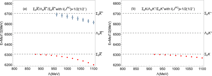
Performing the above procedure, we can systematically investigate the bottom-strange molecular pentaquarks by solving coupled channel Schrödinger equation. In this work, the only free parameter is the UV cutoff $\Lambda$ in Eq. (21), which may vary for different coupled systems being investigated and it lays within the range of $800\sim 5000$ MeV. We firstly deal with bottom baryon $Y_{b}$ and $\bar{K}^{*}$ meson systems to reveal possible bound and resonant states and give them reasonable interpretations. The same technique can be applied in the analysis of bottom baryon $Y_{b}$ and $K$ meson systems. Our estimations for these investigated systems depending on the cutoff value $\Lambda$ are plotted in Figure 2 and listed in Table 3. In the present work, both $S-D$ wave mixing effects and coupled channel effects are taken into account. According to the isospin, spin, and parity, the bottom baryon and anti-strange meson systems can be classified as $1/2(1/2^{-})\Sigma_{b}\bar{K}/\Lambda_{b}\bar{K}^{*}/\Sigma_{b}\bar{K}^{*}$ , $3/2(1/2^{-})\Sigma_{b}\bar{K}/\Sigma_{b}\bar{K}^{*}$ , $1/2(3/2^{-})\Lambda_{b}\bar{K}^{*}/\Sigma_{b}\bar{K}^{*}$ , and $3/2(3/2^{-})\Sigma_{b}\bar{K}^{*}$ channel, respectively. The corresponding classification also exists for the bottom baryon and strange meson systems.

Table 3: The numerical results for the obtained bound states.

	$\Lambda(\rm{MeV})$	$r_{RMS}(\rm{fm})$	$E(\rm{MeV})$	$(\Sigma_{b}\bar{K}(^{2}S_{1/2})$	$\Sigma_{b}\bar{K}^{*}(^{2}S_{1/2})$	$\Sigma_{b}\bar{K}^{*}(^{4}D_{3/2}))$
$I(J^{P})=3/2(1/2^{-})$	3600	3.77	6304.84	(99.08	0.47	0.45)
	3850	1.44	6292.68	(95.75	2.28	1.97)
	4100	1.03	6278.37	(92.78	3.97	3.25)
	$\Lambda(\rm{MeV})$	$r_{RMS}(\rm{fm})$	$E(\rm{MeV})$	( $\Lambda_{b}\bar{K}^{*}(^{4}S_{3/2})$	$\Lambda_{b}\bar{K}^{*}(^{2}D_{3/2})$	$\Lambda_{b}\bar{K}^{*}(^{4}D_{3/2})$	$\Sigma_{b}\bar{K}^{*}(^{4}S_{3/2})$	$\Sigma_{b}\bar{K}^{*}(^{2}D_{3/2})$	$\Sigma_{b}\bar{K}^{*}(^{4}D_{3/2})$ )
$I(J^{P})=1/2(3/2^{-})$	1360	1.69	6509	(0.28	0.25	61.53	36.11	0.06	1.77)
	1380	0.96	6499	(0.34	0.32	45.49	51.00	0.12	2.74)
	1400	0.76	6487	(0.39	0.34	36.98	58.73	0.17	3.39)
	$\Lambda(\rm{MeV})$	$r_{RMS}(\rm{fm})$	$E(\rm{MeV})$	( $\Sigma_{b}\bar{K}^{*}(^{4}S_{3/2})$	$\Sigma_{b}\bar{K}^{*}(^{2}D_{3/2})$	$\Sigma_{b}\bar{K}^{*}(^{4}D_{3/2})$ )
$I(J^{P})=3/2(3/2^{-})$	1300	3.90	6704	(99.26	0.16	0.58)
	1400	2.36	6721	(98.67	0.29	1.04)
	1500	1.61	6697	(98.17	0.40	1.43)
	$\Lambda(\rm{MeV})$	$r_{RMS}(\rm{fm})$	$E(\rm{MeV})$	$(\Sigma_{b}K(^{2}S_{1/2})$	$\Sigma_{b}K^{*}(^{2}S_{1/2})$	$\Sigma_{b}K^{*}(^{4}D_{1/2}))$
$I(J^{P})=3/2(1/2^{-})$	1260	1.51	6298.01	(76.17	23.72	0.10)
	1270	0.90	6284.01	(65.82	34.04	0.15)
	1280	0.67	6265.52	(58.84	41.00	0.16)
	$\Lambda(\rm{MeV})$	$r_{RMS}(\rm{fm})$	$E(\rm{MeV})$	( $\Lambda_{b}K^{*}(^{4}S_{3/2})$	$\Lambda_{b}K^{*}(^{2}D_{3/2})$	$\Lambda_{b}K^{*}(^{4}D_{3/2})$	$\Sigma_{b}K^{*}(^{4}S_{3/2})$	$\Sigma_{b}K^{*}(^{2}D_{3/2})$	$\Sigma_{b}K^{*}(^{4}D_{3/2})$ )
$I(J^{P})=1/2(3/2^{-})$	1260	2.64	6511	(41.20	0.06	40.34	17.16	0.32	0.92)
	1280	1.38	6506	(36.97	0.09	31.78	29.28	0.45	1.43
	1300	0.98	6499	(33.72	0.11	25.67	38.26	0.51	1.73)

III.1 Bottom baryon and anti-strange meson systems

In this subsection, we firstly discuss the coupled $I(J^{PC})=1/2(1/2^{-})$ $\Sigma_{b}\bar{K}/\Lambda_{b}\bar{K}^{*}/\Sigma_{b}\bar{K}^{*}$ systems. As shown in Fig. 2(a), one could find that a bound state and a resonance emerge within the range $\Lambda=880\sim 1100$ $\rm{MeV}$ . When the cutoff $\Lambda$ is set to 880 $\rm{MeV}$ , the bound state locates below $\Sigma_{b}\bar{K}$ threshold with binding energy about $4$ $\rm{MeV}$ , the $r_{RMS}$ is 3 $\rm{fm}$ and dominated by the $\Sigma_{b}\bar{K}(^{2}S_{1/2})$ channel. Sliding the cutoff to $1080$ $\rm{MeV}$ , the mass varies to be around 6222 $\rm{MeV}$ and the $r_{RMS}$ varies to be 0.8 $\rm{fm}$ , which is consistent with the sizes of exotic hadronic molecular state. Thus, this bound state is a good candidate of the particle $\Xi_{b}(6227)$ . These results favors the conclusion in Refs. Huang:2018bed ; Zhu:2020lza ; Mutuk:2024elj . Meanwhile, with the cutoff $\Lambda=970$ $\rm{MeV}$ , we can obtain a resonant state with $E=6693-17i$ $\rm MeV$ and $r_{RMS}=1.70+1.43i$ $\rm{fm}$ , which is mainly composed of the $\Sigma_{b}\bar{K}^{*}(^{2}S_{1/2})$ component. Also, it can be regarded as a good hadronic molecular state. Moreover, our predictions indicate that the pion exchange potential is crucial to form the resonance while the contribution from $\eta$ exchange interaction is negligible. For the $3/2(1/2^{-})$ $\Sigma_{b}\bar{K}^{*}$ state, when the cutoff $\Lambda$ lies in the range of $3360$ to $4100$ $\rm{MeV}$ , a loosely bound state is found with $r_{\text{RMS}}$ varying between $4$ and $1$ $\rm{fm}$ . However, this range for cutoff value is quite different from the empirical value of the deuteron, and then no molecular state is favored in the $3/2(1/2^{-})$ $\Sigma_{b}\bar{K}/\Sigma_{b}\bar{K}^{*}$ system.

Besides, we have $I(J^{P})=1/2(3/2^{-})\Lambda_{b}\bar{K}^{*}/\Sigma_{b}\bar{K}^{*}$ channel for $Y_{b}$ and $\bar{K}^{(*)}$ system, and the corresponding results are listed in Table 3. According to our estimations, a bound state exists below $\Lambda_{b}\bar{K}^{*}$ threshold, dominated by $\Lambda_{b}\bar{K}^{*}(^{4}D_{3/2})$ and $\Sigma_{b}\bar{K}^{*}(^{4}S_{3/2})$ channel, and is sensitive to the cutoff value. Since the cutoff value consists with the empirical value for deuteron, the $I(J^{P})=1/2(3/2^{-})\Lambda_{b}\bar{K}^{*}/\Sigma_{b}\bar{K}^{*}$ can be regarded as a possible molecular state candidate. In the $I(J^{P})=3/2(3/2^{-})$ $\Sigma_{b}\bar{K}^{*}$ system, a weakly bound state with energy of $6703$ $\rm{MeV}$ appears at cutoff $1300$ $\rm{MeV}$ and is dominated by $S-$ wave channel. If only the one pion exchange potential is considered, a bound state is obtain with cutoff $2400$ $\rm{MeV}$ , which means that the potentials of $\rho$ and $\omega$ exchanges are helpful to form the bound state.

III.2 Bottom baryon and strange meson systems

For $Y_{c}K^{(*)}$ systems, the effective potentials from the $\omega$ and $\pi$ exchanges are in completely contrast with $Y_{c}\bar{K}^{(*)}$ systems. Unlike bottom baryon and anti-strange meson systems, for bottom baryon and strange meson systems, one can only obtain bound state solutions. The corresponding numerical results are collected in Table 3 and Figure 2(b). For coupled $\Sigma_{b}K/\Lambda_{b}K^{*}/\Sigma_{b}K^{*}$ with $I(J^{P})=1/2(1/2^{-})$ system, a loosely bound state below $\Sigma_{b}K$ channel is estimated. When the cutoff lies in the range of $920\sim 1100$ MeV, the mass varies from 6304 to 6269 $\rm{MeV}$ and the $r_{RMS}$ decreases from 3 to 1 $\rm{fm}$ , which can be regarded as a good molecular candidate. When the single channel $\Sigma_{b}K$ is considered, one also can obtain a bound state at $\Lambda=1900~{}\rm{MeV}$ that is larger than 920 $\rm{MeV}$ . This foundation also indicates that the coupled channel effect is important to form a molecule. For the $I(J^{P})=3/2(1/2^{-})$ $\Sigma_{b}K/\Sigma_{b}K^{*}$ system, we also obtain a bound state solution when cutoff lies in a range of $1260\sim 1270$ $\rm{MeV}$ . The predicted mass varies from 6298 to 6284 $\rm{MeV}$ and the corresponding $r_{RMS}$ decreases from $1.5$ to $0.9$ $\rm{fm}$ , which is sensitive to cutoff value and may be a molecular state.

As for the $\Lambda_{b}K^{*}/\Sigma_{b}K^{*}$ system with $I(J^{P})=1/2(3/2^{-})$ , at the cutoff is 1260 $\rm MeV$ , a bound state below the $\Lambda_{b}K^{*}$ threshold emerges. One can also find that when only $\Sigma_{b}K^{*}$ channel is considered, a loosely bound state appears, which is listed in Table 3. Finally, for the $I(J^{P})=3/2(3/2^{-})$ $\Sigma_{b}K^{*}$ system, we can not obtain any bound state solution with $\Lambda=800\sim 5000$ MeV.

Table 4: The summary of our predictions for bottom strange pentaquark molecular state systems with cutoff

\Lambda

in a range of

800\sim 1100

\rm MeV

. Here, the ,

"\checkmark"("\times")

represents that the corresponding state may (may not) form a molecular state.

$I(J^{PC})$	Mass $(\rm MeV)$	Width $(\rm MeV)$	$r_{RMS}(\rm fm)$	Status	Selected decay mode
$\frac{1}{2}(\frac{1}{2}^{-})$ $\Sigma_{b}\bar{K}/\Lambda_{b}\bar{K}^{}/\Sigma_{b}\bar{K}^{}$	$6301\sim 6222$	$-$	$2.49\sim 0.73$	$\checkmark$	$\Lambda_{b}\bar{K}/\Xi_{b}^{(\prime)}\pi$
	$6693\sim 6516$	$34.58\sim 31.00$	$1.70+1.43i\sim 0.61+0.51i$	$\checkmark$	$\Lambda_{b}\bar{K}^{()}/\Sigma_{b}\bar{K}/\Lambda\bar{B}^{()}/\Sigma\bar{B}/\Xi_{b}^{(\prime)}\pi/\Xi_{b}^{(\prime)}\eta/\Xi_{b}\rho/\Xi_{b}\omega$
$\frac{3}{2}(\frac{1}{2}^{-})$ $\Sigma_{b}\bar{K}/\Sigma_{b}\bar{K}^{*}$	$-$	$-$	$-$	$\times$	$-$
$\frac{1}{2}(\frac{3}{2}^{-})$ $\Lambda_{b}\bar{K}^{}/\Sigma_{b}\bar{K}^{}$	$-$	$-$	$-$	$\times$	$-$
$\frac{3}{2}(\frac{3}{2}^{-})\Sigma_{b}\bar{K}^{*}$	$6703\sim 6702$	$-$	$3.37\sim 2.62$	$\checkmark$	$\Lambda_{b}\bar{K}^{}/\Sigma_{b}^{}\bar{K}/\Lambda\bar{B}^{}/\Sigma\bar{B}^{}/\Xi_{b}^{}\pi/\Xi_{b}^{}\eta/\Xi_{b}\rho/\Xi_{b}\omega$
$\frac{1}{2}(\frac{1}{2}^{-})$ $\Sigma_{b}K/\Lambda_{b}K^{}/\Sigma_{b}K^{}$	$6303\sim 6269$	$-$	$3.13\sim 1.08$	$\checkmark$	$N\bar{B}_{s}/\Lambda_{b}K$
$\frac{3}{2}(\frac{1}{2}^{-})$ $\Sigma_{b}K/\Sigma_{b}K^{*}$	$-$	$-$	$-$	$\times$	$-$
$\frac{1}{2}(\frac{3}{2}^{-})$ $\Lambda_{b}K^{}/\Sigma_{b}K^{}$	$-$	$-$	$-$	$\times$	$-$
$\frac{3}{2}(\frac{3}{2}^{-})$ $\Sigma_{b}K^{*}$	$6704\sim 6692$	$-$	$4.13\sim 1.34$	$\checkmark$	$N\bar{B}_{s}^{}/\Lambda_{b}^{}K/\Sigma_{b}^{*}K$

III.3 Further discussions

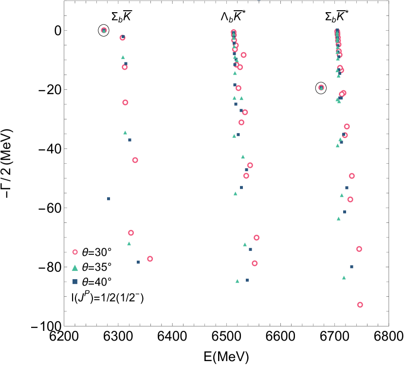
For $Y_{b}\bar{K}^{(*)}$ systems, we can obtain bound states and resonances, but only bound states are revealed for $Y_{b}K^{(*)}$ systems. The reason is that the flavor factors in the potentials for these systems are quite different, which determine the relative sign and strength and are crucial for the formation of molecular states. It is also interesting to note that the root mean square (RMS) radius $r_{RMS}$ for the $I(J^{PC})=1/2(1/2^{-})\Sigma_{b}\bar{K}/\Lambda_{b}\bar{K}^{*}/\Sigma_{b}\bar{K}^{*}$ resonances can be a complex number. In such cases, one can use the interpretation scheme proposed by T. Berggren, which generalizes the concept of expectation values from bound states to resonances Berggren:1970wto . According to this scheme, the real part of the complex $r_{RMS}$ represents the usual physical expectation value, while the imaginary part indicates a measure of uncertainty in the observation. Numerical calculations of $r^{2}$ have supported this generalized interpretation Gyarmati:1972yac ; 1997matrix . We illustrate the The complex energy eigenvalues of $I(J^{P})=1/2(1/2^{-})$ system with varying the angle $\theta$ from $30^{\circ}\sim 40^{\circ}$ in Figure 3.

According to the masses and quantum numbers, we present some possible decay channels for these predicted states in Table 4. For instance, the $I(J^{PC})=1/2(1/2^{-})$ $\Sigma_{b}\bar{K}/\Lambda_{b}\bar{K}^{*}/\Sigma_{b}\bar{K}^{*}$ bound state can be found in $\Lambda_{b}\bar{K}$ and $\Xi_{b}^{(\prime)}\pi$ channels. In the literature Chen:2018orb ; He:2021xrh ; Wang:2018fjm ; Cui:2019dzj , both $J^{P}=\frac{1}{2}^{-}$ molecular and $J^{P}=\frac{3}{2}^{-}/\frac{5}{2}^{-}$ conventional interpretations exist for the particle $\Xi_{b}(6227)$ , and the spin is certainly crucial for distinguishing these two explanations. Another way to solve this puzzle is to hunt for the flavor exotic state with $6303\sim 6269~{}\rm{MeV}$ in the $I(J^{PC})=1/2(1/2^{-})$ $\Sigma_{b}K/\Lambda_{b}K^{*}/\Sigma_{b}K^{*}$ system, which is the mirror state of $\Xi_{b}(6227)$ in the molecular picture but does not appear in the three-quark picture. We highly hope that the future experiments can verify our proposals.

IV Summary

In this work, we systematically investigate the coupled $Y_{b}\bar{K}^{(*)}(Y_{b}K^{(*)})$ system to search for possible bound states and resonances by adopting one-boson-exchange model within complex scaling method. For the coupled $I(J^{P})=1/2(1/2^{-})$ $\Sigma_{b}\bar{K}/\Lambda_{b}\bar{K}^{*}/\Sigma_{b}\bar{K}^{*}$ systems, according to our estimations, a bound state solution is obtained, which may correspond to the observed particle $\Xi_{b}(6227)$ . Meanwhile, we find a $I(J^{PC})=1/2(1/2^{-})$ resonance near the $\Sigma_{b}\bar{K}^{*}$ threshold and a bound state in the $I(J^{P})=1/2(3/2^{-})$ $\Sigma_{b}\bar{K}^{*}$ system.

Then, when we extend our study to the $Y_{b}K^{(*)}$ systems, two loosely bound states are obtained. It is worth pointing out that the predicted bound state with $6303\sim 6269~{}\rm{MeV}$ in the $I(J^{P})=1/2(1/2^{-})$ $\Sigma_{b}K/\Lambda_{b}K^{*}/\Sigma_{b}K^{*}$ system is flavor exotic and does not appear in the spectroscopy of conventional baryons, which provides a practical way to resolve the puzzle of particle $\Xi_{b}(6227)$ . We hope our predictions can offer valuable information to the future experiments observations.

ACKNOWLEDGMENTS

We would like to thank Rui Chen, Xian-Hui Zhong, Li-Cheng Sheng, and Jin-Yu Huo for useful discussions. The work of X.-N. X. and Q. F. Song is supported by the National Natural Science Foundation of China under Grants No. 12275364. Q.-F. Lü is supported by the Natural Science Foundation of Hunan Province under Grant No. 2023JJ40421, the Scientific Research Projects of Hunan Provincial Education Department under Grant No. 24B0063, and the Youth Talent Support Program of Hunan Normal University under Grant No. 2024QNTJ14.

References

(1) S. K. Choi et al. (Belle Collaboration), Observation of a narrow charmonium-like state in exclusive $B^{\pm}\to K^{\pm}\pi^{+}\pi^{-}J/\psi$ decays, Phys. Rev. Lett. 91, 262001 (2003).
(2) Y. R. Liu, H. X. Chen, W. Chen, X. Liu and S. L. Zhu, Prog. Part. Nucl. Phys. 107, 237-320 (2019) doi:10.1016/j.ppnp.2019.04.003 [arXiv:1903.11976 [hep-ph]].
(3) X. H. Liu, Q. Wang and Q. Zhao, Phys. Lett. B 757, 231-236 (2016) doi:10.1016/j.physletb.2016.03.089 [arXiv:1507.05359 [hep-ph]].
(4) H. X. Chen, W. Chen, X. Liu, Y. R. Liu and S. L. Zhu, An updated review of the new hadron states, Rept. Prog. Phys. 86, 026201 (2023).
(5) M. Mai, U. G. Meißner and C. Urbach, Towards a theory of hadron resonances, Phys. Rept. 1001, 1-66 (2023).
(6) F. K. Guo, C. Hanhart, U. G. Meißner, Q. Wang, Q. Zhao and B. S. Zou, Hadronic molecules, Rev. Mod. Phys. 90, 015004 (2018).
(7) M. Karliner, J. L. Rosner and T. Skwarnicki, Multiquark States, Ann. Rev. Nucl. Part. Sci. 68, 17 (2018).
(8) Y. Dong, A. Faessler and V. E. Lyubovitskij, Description of heavy exotic resonances as molecular states using phenomenological Lagrangians, Prog. Part. Nucl. Phys. 94, 282 (2017).
(9) B. S. Zou, Hadron spectroscopy from strangeness to charm and beauty, Nucl. Phys. A 914, 454-460 (2013).
(10) B. S. Zou, Building up the spectrum of pentaquark states as hadronic molecules, Sci. Bull. 66, 1258 (2021).
(11) R. Aaij et al. [LHCb], Phys. Rev. Lett. 125, 242001 (2020) doi:10.1103/PhysRevLett.125.242001 [arXiv:2009.00025 [hep-ex]].
(12) R. Aaij et al. [LHCb], Phys. Rev. D 102, 112003 (2020) doi:10.1103/PhysRevD.102.112003 [arXiv:2009.00026 [hep-ex]].
(13) H. X. Chen, W. Chen, R. R. Dong and N. Su, Chin. Phys. Lett. 37, no.10, 101201 (2020) doi:10.1088/0256-307X/37/10/101201 [arXiv:2008.07516 [hep-ph]].
(14) J. He and D. Y. Chen, Chin. Phys. C 45, no.6, 063102 (2021) doi:10.1088/1674-1137/abeda8 [arXiv:2008.07782 [hep-ph]].
(15) T. J. Burns and E. S. Swanson, Phys. Lett. B 813, 136057 (2021) doi:10.1016/j.physletb.2020.136057 [arXiv:2008.12838 [hep-ph]].
(16) S. S. Agaev, K. Azizi and H. Sundu, J. Phys. G 48, no.8, 085012 (2021) doi:10.1088/1361-6471/ac0b31 [arXiv:2008.13027 [hep-ph]].
(17) C. J. Xiao, D. Y. Chen, Y. B. Dong and G. W. Meng, Phys. Rev. D 103, no.3, 034004 (2021) doi:10.1103/PhysRevD.103.034004 [arXiv:2009.14538 [hep-ph]].
(18) H. W. Ke, Y. F. Shi, X. H. Liu and X. Q. Li, Phys. Rev. D 106, no.11, 114032 (2022) doi:10.1103/PhysRevD.106.114032 [arXiv:2210.06215 [hep-ph]].
(19) R. Aaij et al. [LHCb], Phys. Rev. Lett. 131, no.4, 041902 (2023) doi:10.1103/PhysRevLett.131.041902 [arXiv:2212.02716 [hep-ex]].
(20) R. Aaij et al. [LHCb], Phys. Rev. D 108, no.1, 012017 (2023) doi:10.1103/PhysRevD.108.012017 [arXiv:2212.02717 [hep-ex]].
(21) B. Wang, K. Chen, L. Meng and S. L. Zhu, Phys. Rev. D 109, no.3, 034027 (2024) doi:10.1103/PhysRevD.109.034027 [arXiv:2309.02191 [hep-ph]].
(22) S. S. Agaev, K. Azizi and H. Sundu, Phys. Rev. D 107, no.9, 094019 (2023) doi:10.1103/PhysRevD.107.094019 [arXiv:2212.12001 [hep-ph]].
(23) H. T. An, Z. W. Liu, F. S. Yu and X. Liu, Phys. Rev. D 106, no.11, L111501 (2022) doi:10.1103/PhysRevD.106.L111501 [arXiv:2207.02813 [hep-ph]].
(24) V. M. Abazov et al. [D0], Phys. Rev. Lett. 117, no.2, 022003 (2016) doi:10.1103/PhysRevLett.117.022003 [arXiv:1602.07588 [hep-ex]].
(25) R. Aaij et al. [LHCb], Phys. Rev. Lett. 117, no.15, 152003 (2016) doi:10.1103/PhysRevLett.117.152003 [arXiv:1608.00435 [hep-ex]].
(26) M. Aaboud et al. [ATLAS], Phys. Rev. Lett. 120, no.20, 202007 (2018) doi:10.1103/PhysRevLett.120.202007 [arXiv:1802.01840 [hep-ex]].
(27) T. Aaltonen et al. [CDF], Phys. Rev. Lett. 120, no.20, 202006 (2018) doi:10.1103/PhysRevLett.120.202006 [arXiv:1712.09620 [hep-ex]].
(28) A. M. Sirunyan et al. [CMS], Phys. Rev. Lett. 120, no.20, 202005 (2018) doi:10.1103/PhysRevLett.120.202005 [arXiv:1712.06144 [hep-ex]].
(29) R. Chen and X. Liu, Phys. Rev. D 94, no.3, 034006 (2016) doi:10.1103/PhysRevD.94.034006 [arXiv:1607.05566 [hep-ph]].
(30) C. J. Xiao and D. Y. Chen, Eur. Phys. J. A 53, no.6, 127 (2017) doi:10.1140/epja/i2017-12310-x [arXiv:1603.00228 [hep-ph]].
(31) S. S. Agaev, K. Azizi and H. Sundu, Eur. Phys. J. Plus 131, no.10, 351 (2016) doi:10.1140/epjp/i2016-16351-8 [arXiv:1603.02708 [hep-ph]].
(32) R. Aaij et al. [LHCb], Eur. Phys. J. C 81, no.7, 601 (2021) doi:10.1140/epjc/s10052-021-09305-3 [arXiv:2010.15931 [hep-ex]].
(33) S. Y. Kong, J. T. Zhu, D. Song and J. He, Phys. Rev. D 104, no.9, 094012 (2021) doi:10.1103/PhysRevD.104.094012 [arXiv:2106.07272 [hep-ph]].
(34) E. E. Kolomeitsev and M. F. M. Lutz, Phys. Lett. B 582, 39-48 (2004) doi:10.1016/j.physletb.2003.10.118 [arXiv:hep-ph/0307133 [hep-ph]].
(35) F. K. Guo, P. N. Shen, H. C. Chiang, R. G. Ping and B. S. Zou, Phys. Lett. B 641, 278-285 (2006) doi:10.1016/j.physletb.2006.08.064 [arXiv:hep-ph/0603072 [hep-ph]].
(36) F. K. Guo, P. N. Shen and H. C. Chiang, Phys. Lett. B 647, 133-139 (2007) doi:10.1016/j.physletb.2007.01.050 [arXiv:hep-ph/0610008 [hep-ph]].
(37) Z. F. Sun, J. J. Xie and E. Oset, Phys. Rev. D 97, no.9, 094031 (2018) doi:10.1103/PhysRevD.97.094031 [arXiv:1801.04367 [hep-ph]].
(38) T. Asanuma, Y. Yamaguchi and M. Harada, [arXiv:2311.04695 [hep-ph]].
(39) M. Tanaka, Y. Yamaguchi and M. Harada, Phys. Rev. D 110, no.1, 016024 (2024) doi:10.1103/PhysRevD.110.016024 [arXiv:2403.03548 [hep-ph]].
(40) B. Wang, K. Chen, L. Meng and S. L. Zhu, Phys. Rev. D 109, no.7, 074035 (2024) doi:10.1103/PhysRevD.109.074035 [arXiv:2312.13591 [hep-ph]].
(41) M. Sakai and Y. Yamaguchi, Phys. Rev. D 109, no.5, 054016 (2024) doi:10.1103/PhysRevD.109.054016 [arXiv:2312.08663 [hep-ph]].
(42) R. Chen and Q. Huang, [arXiv:2208.10196 [hep-ph]].
(43) R. Aaij et al. [LHCb], Phys. Rev. Lett. 121, No.7, 072002 (2018).
(44) B. Chen, K. W. Wei, X. Liu and A. Zhang, Phys. Rev. D 98, No.3, 031502 (2018).
(45) H. Z. He, W. Liang, Q. F. Lü and Y. B. Dong, Sci. China Phys. Mech. Astron. 64, No.6, 261012 (2021).
(46) K. L. Wang, Q. F. Lü and X. H. Zhong, Phys. Rev. D 99, No.1, 014011 (2019).
(47) E. L. Cui, H. M. Yang, H. X. Chen and A. Hosaka, Phys. Rev. D 99, No.9, 094021 (2019).
(48) H. Z. He, W. Liang, Q. F. Lü and Y. B. Dong, Sci. China Phys. Mech. Astron. 64, no.6, 261012 (2021) doi:10.1007/s11433-021-1704-x [arXiv:2102.07391 [hep-ph]].
(49) Y. Huang, C. j. Xiao, L. S. Geng and J. He, Phys. Rev. D 99, No.1, 014008 (2019).
(50) H. Zhu and Y. Huang, Chin. Phys. C 44, No.8, 083101 (2020).
(51) H. Mutuk, Magnetic Moment of $\Xi_{b}(6227)$ as Molecular Pentaquark State,[arXiv:2403.13896 [hep-ph]].
(52) Q. F. Song, Q. F. Lü, D. Y. Chen and Y. B. Dong, Phys. Rev. D 110, no.7, 074038 (2024) doi:10.1103/PhysRevD.110.074038 [arXiv:2405.07694 [hep-ph]].
(53) Y. K. Ho, The method of complex coordinate rotation and its applications to atomic collision processes, Phys. Rept. 99, 1-68 (1983).
(54) N. Moiseyev, Quantum theory of resonances: calculating energies, widths and cross-sections by complex scaling, Phys. Rept. 302, 212-293 (1998).
(55) E. Hiyama, Y. Kino and M. Kamimura, Prog. Part. Nucl. Phys. 51, 223-307 (2003).
(56) E. Hiyama and M. Kamimura, Study of various few-body systems using Gaussian expansion method (GEM), Front. Phys. (Beijing) 13, 132106 (2018).
(57) Y. R. Liu and M. Oka, Phys. Rev. D 85, 014015 (2012) doi:10.1103/PhysRevD.85.014015 [arXiv:1103.4624 [hep-ph]].
(58) R. Chen, A. Hosaka and X. Liu, Phys. Rev. D 97, no.3, 036016 (2018) doi:10.1103/PhysRevD.97.036016 [arXiv:1711.07650 [hep-ph]].
(59) O. Kaymakcalan, S. Rajeev and J. Schechter, Phys. Rev. D 30, 594 (1984) doi:10.1103/PhysRevD.30.594
(60) J. Aguilar and J. M. Combes, Commun. Math. Phys. 22, 269-279 (1971) doi:10.1007/BF01877510
(61) E. Balslev and J. M. Combes, Commun. Math. Phys. 22, 280-294 (1971) doi:10.1007/BF01877511
(62) M. Homma, T. Myo, and K. Katō, Matrix elements of physical quantities associated with resonance states, Prog. Theor. Phys. 97, 561 (1997).
(63) Z. Y. Lin, J. B. Cheng, B. L. Huang and S. L. Zhu, Partial widths from analytical extension of the wave function: $P_{c}$ states, Phys. Rev. D 108, 114014 (2023).
(64) Y. Shimizu, D. Suenaga and M. Harada, Coupled channel analysis of molecule picture of $P_{c}(4380)$ , Phys. Rev. D 93, 114003 (2016).
(65) T. Myo, Y. Kikuchi, H. Masui and K. Katō, Recent development of complex scaling method for many-body resonances and continua in light nuclei, Prog. Part. Nucl. Phys. 79, 1-56 (2014).
(66) T. Berggren, On a probabilistic interpretation of expansion coefficients in the non-relativistic quantum theory of resonant states, Phys. Lett. B 33, 547-549 (1970).
(67) B. Gyarmati, F. Krisztinkovics and T. Vertse, On the expectation value in Gamow state, Phys. Lett. B 41, 110-112 (1972).
(68) M. Homma, T. Myo, K. Katō, Prog. Matrix elements of physical quantities associated with resonance states, Theor. Phys. 97 (1997) 561.
(69) Z. W. Lin and C. M. Ko, A Model for $J/\psi$ absorption in hadronic matter, Phys. Rev. C 62, 034903 (2000).