A CUBESAT FOR CALIBRATING GROUND-BASED AND SUB-ORBITAL MILLIMETER-WAVE POLARIMETERS (CALSAT)
Abstract
We describe a low-cost, open-access, CubeSat-based calibration instrument that is designed to support ground-based and sub-orbital experiments searching for various polarization signals in the cosmic microwave background (CMB). All modern CMB polarization experiments require a robust calibration program that will allow the effects of instrument-induced signals to be mitigated during data analysis. A bright, compact, and linearly polarized astrophysical source with polarization properties known to adequate precision does not exist. Therefore, we designed a space-based millimeter-wave calibration instrument, called CalSat, to serve as an open-access calibrator, and this paper describes the results of our design study. The calibration source on board CalSat is composed of five “tones” with one each at 47.1, 80.0, 140, 249 and 309 GHz. The five tones we chose are well matched to (i) the observation windows in the atmospheric transmittance spectra, (ii) the spectral bands commonly used in polarimeters by the CMB community, and (iii) The Amateur Satellite Service bands in the Table of Frequency Allocations used by the Federal Communications Commission. CalSat will be placed in a polar orbit allowing visibility from observatories in the Northern Hemisphere, such as Mauna Kea in Hawaii and Summit Station in Greenland, and the Southern Hemisphere, such as the Atacama Desert in Chile and the South Pole. CalSat also will be observable by balloon-borne instruments launched from a range of locations around the world. This global visibility makes CalSat the only source that can be observed by all terrestrial and sub-orbital observatories, thereby providing a universal standard that permits comparison between experiments using appreciably different measurement approaches.
keywords:
CMB Polarization, CubeSat, Calibration, B-modes.; ; ;
1 Introduction
In this paper, we describe a low-cost, open-access, CubeSat-based calibration instrument called CalSat that is designed to support ground-based and sub-orbital experiments searching for various polarization signals in the cosmic microwave background (CMB). The CMB is a bath of photons that permeates all of space and carries an image of the Universe as it was 380,000 years after the Big Bang. This image spans the entire sky, but it is not visible to the human eye because the frequency spectrum of the CMB peaks in the millimeter-wave region of the electromagnetic spectrum. Physical processes that operated in the universe when the CMB formed left an imprint that can be detected today. This imprint is observed as angular intensity and linear polarization anisotropies. These primordial CMB anisotropies have proven to be a treasure trove of cosmological information. For example, the precise characterization of the intensity (or temperature) anisotropy of the CMB has helped reveal that spacetime is flat, the universe is 13.8 billion years old, and the energy content of the universe is dominated by cold dark matter and dark energy [see for example, Bennett et al., 2013; Planck Collaboration, 2014]. The density inhomogeneities that produced the detected temperature anisotropies theoretically should generate, through Thomson scattering during the epoch of recombination, a curl-free polarization signal known as “E-mode” polarization. This companion signal has also been observed at the theoretically expected level providing further confidence in the CDM cosmological model [see for example, Naess et al., 2014; Crites et al., 2015; BICEP2 Collaboration, 2014a; QUIET Collaboration, 2011; Brown et al., 2009].
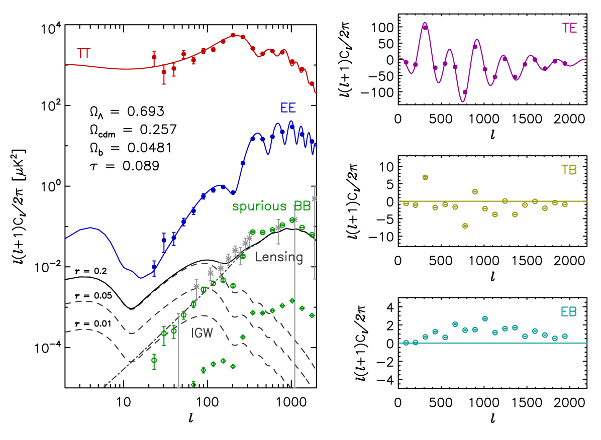
The inflationary cosmological paradigm posits that a burst of exponential spacetime expansion, called inflation, took place during the first fraction of a second after the Big Bang. Observational evidence to date supports this paradigm and has given it a strong footing, though the precise physical mechanism that caused inflation is unknown. Inflation should have produced a stochastic background of gravitational waves. These gravitational waves would have produced polarization signals separable from E-modes by their divergence-free “B-mode” signature Zaldarriaga & Seljak [1997]; Kamionkowski et al. [1997]. The magnitude of this inflationary gravitational wave (IGW) B-mode signal is proportional to the energy scale at which inflation occurred. See for example, the dashed curves in Figure 1 and note that the IGW signal amplitude is commonly parameterized as , the so-called tensor-to-scalar ratio, which is related to the energy scale of inflation111The tensor-to-scalar ratio is related to the energy scale of inflation as [GeV]. Baumann et al. [2009]; Knox & Song [2002]. If the IGW signal ultimately is discovered, then the energy scale of inflation would be experimentally ascertained. This measurement would place a tight constraint on the theoretical models that describe the inflation mechanism, and this constraint would be a breakthrough for both astrophysics and particle physics because there is no way to create inflation-like conditions in a laboratory or particle accelerator. The IGW signal is currently the primary focus of CMB research, and we will discuss the status of current measurements at the end of Section 2.
In addition to the IGW signal, other CMB polarization signals promise to deliver valuable cosmological information. Non-primordial B-modes are generated when E-modes are gravitationally lensed by large-scale structures in the Universe (see the dash-dot curve in Figure 1). This lensing B-mode signal is sensitive to physical parameters such as the sum of the neutrino masses Abazajian et al. [2015a]. B-mode polarization can also be used to probe physics outside the standard cosmological picture. Temperature to B-mode correlations (TB) and E-mode and B-mode correlations (EB) are expected to vanish in the standard model. Therefore, these estimators are sensitive probes for physics outside the standard model if the correlation signals are found to be non-zero. A variety of candidate non-standard-model physical mechanisms that produce cosmological polarization rotation (CPR) already have been identified. Parity violation in the electromagnetic sector via a Chern-Simons coupling can produce TB and EB correlations Kaufman et al. [2014]. A coupling of a pseudo-scalar field to electromagnetism would violate the Einstein Equivalence Principle and would result in TB and EB correlations Ni [1977]; Carroll et al. [1991]. TB and EB correlations can also be used to test chiral gravity models Gluscevic & Kamionkowski [2010] and to search for primordial magnetic fields Pogosian et al. [2009]; Yadav et al. [2012].
| frequency | polarization angle uncertainty | total power | polarized power | |||||
| [GHz] | [Jy] | [Jy] | [%] | systematic [deg] | statistical [deg] | [fW] | [fW] | |
| Planck | 30 | 340 | 24 | 7.1 | 0.50 | 0.54 | 16 | 2.2 |
| 44 | 290 | 19 | 6.5 | 0.50 | 0.32 | 20 | 2.5 | |
| 70 | 260 | 21 | 7.9 | 0.50 | 0.23 | 30 | 4.4 | |
| 100 | 220 | 16 | 7.2 | 0.62 | 0.11 | 35 | 4.8 | |
| 143 | 170 | 12 | 7.2 | 0.62 | 0.13 | 39 | 5.1 | |
| 217 | 120 | 10 | 8.1 | 0.62 | 0.12 | 42 | 6.5 | |
| 353 | 82 | 10 | 12 | 0.62 | 0.37 | 49 | 11 | |
| WMAP | 23 | 380 | 27 | 7.1 | 1.5 | 0.10 | 14 | 1.9 |
| 33 | 340 | 24 | 6.9 | 1.5 | 0.10 | 18 | 2.4 | |
| 41 | 320 | 22 | 7.0 | 1.5 | 0.20 | 21 | 2.7 | |
| 61 | 280 | 19 | 7.0 | 1.5 | 0.40 | 27 | 3.5 | |
| 93 | 230 | 17 | 7.1 | 1.5 | 0.70 | 34 | 4.7 | |
| IRAM | 90 | 200 | 15 | 8.8 | 0.50 | 0.20 | 29 | 4.7 |
| CalSat | 47.1 | 100 | 0.05 | 2000 | 2000 | |||
| 80.0 | 100 | 0.05 | 1300 | 1300 | ||||
| 140 | 100 | 0.05 | 130 | 130 | ||||
| 249 | 100 | 0.05 | 48 | 48 | ||||
| 309 | 100 | 0.05 | 23 | 23 | ||||
-
Measurements from Planck Collaboration [2015] using the maximum likelihood filtering method
-
Measurements from Weiland et al. [2011]
-
Measurement from Aumont et al. [2010]
-
Computed for this comparison assuming the detector is sensitive to a single polarization and the telescope aperture area is 1 m2 for all cases. To convert the measurements from Planck, WMAP and IRAM from Jy to fW, we made the additional assumption that
2 Polarimeter Calibration
The magnitude of the forecasted TB, EB and B-mode signals is faint when compared with unavoidable instrument-induced systematic errors. Therefore, all experiments trying to measure these signals need a robust polarimeter calibration program that will allow the effect of these instrument-induced errors to be mitigated during data analysis. Several performance requirement studies have been published specifically for IGW searches Bock et al. [2006]; O’Dea et al. [2007]; Bock et al. [2009]. These studies indicate the level of systematic error that can be tolerated for a given IGW signal amplitude. For the CalSat design program we chose to use the performance requirements derived by the Task Force on Cosmic Microwave Background Research Bock et al. [2006] as a benchmark. This report proposes a general performance requirement where each systematic error must be suppressed to a factor of ten below an IGW signal corresponding to a tensor-to-scalar ratio of , which is the level where the gravitational lensing signal starts to dominate the IWG signal at .
Many of the known systematic errors can be mitigated straightforwardly. However, a robust mitigation strategy for instrument-induced polarization rotation (IPR), which is one of the most critical systematic errors, has not yet been identified. This instrumental effect rotates the apparent orientation of the linearly-polarized pseudo-vectors on the sky, and this rotation converts the brighter E-modes into spurious B-modes. Using the aforementioned performance requirement definition, any IPR must be limited to 0.2 deg for an IGW search targeting ; fainter IGW signals would require a tighter constraint, and even more precision could be needed if delensing techniques ultimately will be used to probe below Smith et al. [2012].
To illustrate this effect we performed a simple experiment simulation where a set of Stokes parameter maps (, , with ) containing CMB signals were simulated and then the orientation of the polarization of each pixel was rotated by 2 deg using the Mueller matrix for linear polarization rotation. The input maps were 1000 deg2, contained no noise or other beam effects, and all B-mode signals were set to zero. The angular power spectra of the corrupted maps were then estimated, and the estimated power spectra are shown in Figure 1. The open-circle points in this figure (BB, TB and EB) are spurious signals entirely produced by the polarization rotation operation. A rotation of just 2 deg creates a false B-mode signal that is comparable in magnitude to both the lensing signal and the sought-after IGW signal below if the tensor-to-scalar ratio is . The takeaway message is a very small amount of rotation can produce a false B-mode signal that can obscure the actual sky signal.
To properly characterize the IPR properties of a CMB polarimeter, a linearly polarized source with known polarization properties should be observed with high precision. This required calibration measurement provides the critical relationship between the coordinate system of the polarimeter in the instrument frame and the coordinate system on the sky that defines the astrophysical and Stokes parameters. The ideal source should be point-like in the beam of the telescope and bright enough to generate high signal-to-noise calibration data with a reasonable amount of integration time. But this source should not be too bright, or it will saturate the detector system. Finally, the orientation of the polarization of the observed source on the sky must be known to 0.2 deg or better for . It is important to note that the magnitude of this systematic error typically varies across the focal plane of the telescope, so the IPR effect must be determined for each detector in any given instrument.
Many current experiments “self-calibrate” their polarization angles by assuming TB and EB correlations are zero Keating et al. [2013]. This self-calibration technique uses the TB and EB spectra on the right in Figure 1 along with the theoretical idea that these spectra should be zero in the absence of CPR to remove the green spurious B-mode points on the left. This approach makes it impossible to use B-mode, TB and EB measurements to constrain the aforementioned isotropic departures from the standard model (see Section 1) because any signal produced by CPR is incorrectly interpreted as an error signal. If this problem is avoided and self-calibration is not used, then the current achieved precision of 0.5 deg severely limits the ability of experiments to search for any departures from standard cosmology via TB and EB measurements. A more precise calibration procedure is needed to make progress with CPR studies.
Some partially polarized astrophysical sources are available, and at millimeter-wavelengths, the best of these appears to be Tau A. Tau A is a supernova remnant located at Right ascension = 05 34 32 (hms) and Declination = +22 00 52 (dms), and it has an angular extent of . For calibration, its most relevant properties are (i) the measured polarization angle uncertainty, (ii) the polarized fraction, and (iii) the source brightness. The WMAP satellite measured its polarization properties in spectral bands between 20 and 100 GHz Weiland et al. [2011], the Planck satellite measured its polarization properties in spectral bands between 30 and 353 GHz Planck Collaboration [2015], and Aumont et al. [2010] studied the suitability of Tau A as a calibration source for CMB studies at 90 GHz using the 30 m IRAM telescope. These measurements are summarized in Table 1. ACTpol Naess et al. [2014] and POLARBEAR POLARBEAR Collaboration [2014] recently observed Tau A as part of their respective calibration programs and showed that the polarization intensity morphology at 145 GHz is complicated.
Though Tau A is the best polarized source on the sky at millimeter wavelengths, it does not meet the performance requirements of a calibrator for an IGW-signal search. First and foremost, with a Declination = +22 00 52 (dms), it is not accessible to observatories at the South Pole or on Antarctic balloons. It can be observed from the Atacama Desert in Chile, though it will always be at a zenith angle of 45 deg or more. Second, it is not bright enough to give a high signal-to-noise ratio measurement with a short integration time. Third, the source is extended rather than point-like. And finally, the millimeter-wave spectrum of Tau A is not precisely known, though it is certainly not that of a 2.7 K blackbody. Polarimeters that have frequency-dependent performance, which is common, would need to precisely measure the frequency spectrum of Tau A before using it as a polarization angle calibrator (see Section 4).
Since an ideal celestial calibration source does not exist, some current experiments use ground-based sources for polarimeter calibration BICEP2 Collaboration [2014b]; Crites et al. [2015]. However, these measurements are challenging. For example, the Fraunhofer distance () for common telescopes is typically between 0.1 and 100 km, so the calibration source must be placed more than 0.1 to 100 km away, respectively, from the telescope for the desired far-field beam characterization measurement. This kind of measurement is difficult because the detector systems in CMB polarimeters are designed to observe sky backgrounds, which are typically 10 K or less. To observe a ground-based calibration source more than 0.1 to 100 km away, the zenith angle of the telescope must be set to nearly 90 deg. Background loading from the large airmass and thermal emission from the ground at this zenith angle are high enough to saturate typical detector systems222Here we are assuming bolometric detectors are being used. Bolometers are commonly used in CMB observations.. Therefore two-stage bolometers or some kind of signal attenuator must be used for this style of calibration measurement. However, these approaches have their own varieties of systematic error, so awkwardly these calibration measurements could require their own calibration. A near-field measurement of a calibration source observed at smaller zenith angles can be performed instead to mitigate this high background loading problem. Yet, for the near-field measurement to be useful, a model-dependent theoretical correction must be applied to the data to derive the effective far-field calibration. This correction, however, also introduces uncertainty into the calibration, and the quality of the result depends entirely on the accuracy of this difficult theoretical calculation.
Current experiments are beginning to measure B-modes. The BICEP2 Collaboration recently announced a detection of degree-scale B-mode polarization in a 350 deg2 patch of sky in the southern hemisphere BICEP2 Collaboration [2014a]. The POLARBEAR and SPTPol Collaborations detected B-mode polarization consistent with the aforementioned gravitational lensing signal on sub-degree scales POLARBEAR Collaboration [2014]; Keisler et al. [2015]. And the Planck Collaboration published a measurement of B-mode polarization from Galactic dust emission at 353 GHz Adam et al. [2014]. This combination of results has added energy to CMB studies because these measurements indicate that faint B-mode signals are there on the sky and that instruments are now sensitive enough to detect them. Currently, BICEP2 and POLARBEAR use the aforementioned self-calibration technique, so it impossible to use these measurements to constrain isotropic departures from the standard model. These results have re-emphasized the need for enhanced foreground discrimination capabilities and robust systematic error control; the latter effect being the major motivation behind CalSat.
3 Technical Approach
3.1 What are CubeSats?
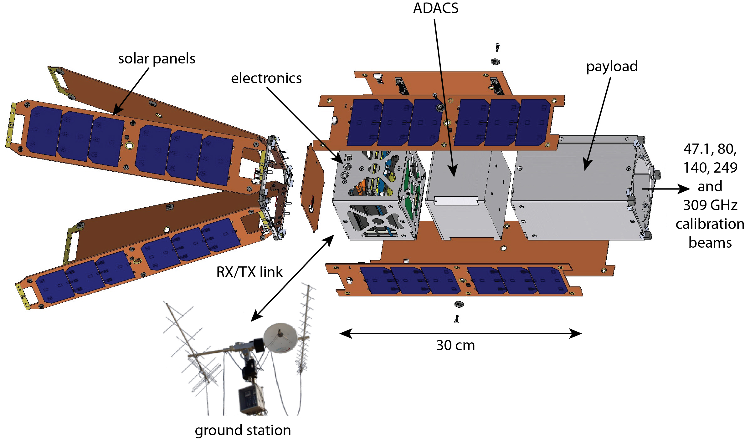
A CubeSat-based instrument like the one we designed is composed of a “bus,” a payload and a ground station. These components can be seen in Figure 2. The bus includes the mechanical frame, the power system, solar panels, the on-board computer and electronics, an attitude determination and control system (ADACS), and a transmitter/receiver. The payload is the scientific experiment, which is mounted inside the bus. For CalSat the payload is the calibration instrument. The ground station includes a transmitter/receiver and computers, and it is used to download data and upload commands. It serves as the point of contact between the research team and the orbiting spacecraft.
CubeSats essentially get a free ride into orbit as auxiliary payloads. A Poly Picosatellite Orbital Deployer (P-POD) is installed in a rocket alongside its primary payload. CubeSats are loaded into the P-POD, and the P-POD jettisons the CubeSats at the appropriate time after launch. The P-POD defines the CubeSat standard, and CubeSats must conform to a strict list of requirements333CubeSat requirements document: http://www.cubesat.org/index.php/documents/developers so that they are compatible with the P-POD. Among these requirements is a volume requirement. The fundamental CubeSat size is 10 cm 10 cm 10 cm, and this size is referred to as “1U,” but larger 2U (10 cm 10 cm 20 cm) and 3U (10 cm 10 cm 30 cm) sizes also can fit into the P-POD.
| Characteristic | Value |
|---|---|
| source frequencies [GHz] | 47.1, 80.0, 140, 249 and 309 |
| source spectral width [MHz] | |
| output millimeter-wave power [mW] | 50, 40, 3.2, 1.2 and 0.45 |
| polarization | linear |
| cross-polarization level [dB] | -60 |
| horn type | conical |
| input waveguide on horn | rectangular, single-moded |
| horn gain [dBi] | approximately 20 |
| ADACS steering uncertainty [deg] | 1 |
| ADACS attitude measurement uncertainty [deg] | 0.05 |
| polarization orientation uncertainty [deg] | 0.05 |
| estimated payload mass [kg] | 0.8 |
| estimated total CubeSat mass [kg] | 3.8 |
| calculated operating temperature [∘C] | 10 (night) to 30 (day) |
| orbit altitude [km] | 500 |
| orbital period [hours] | 1.6 |
| orbits per day | 14.2 |
3.2 CalSat Description
CalSat is based on a 3U CubeSat, and all of the required CubeSat hardware is commercially available. The primary CalSat characteristics are summarized in Table 2.
3.2.1 Bus/ADACS
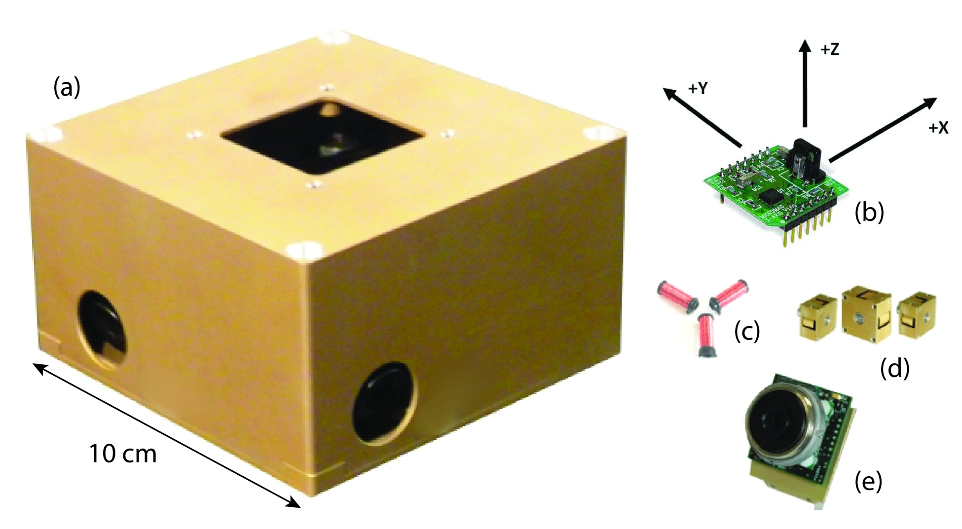
The CalSat design uses the MISC3 3U CubeSat bus from Pumpkin Inc., which is a turnkey CubeSat kit that includes all of the aforementioned bus components. Pumpkin Incorporated was selected as the bus supplier for CalSat because their bus meets the pointing performance specification and more than ten of their CubeSats already have been successfully launched, therefore their hardware is well tested and comparatively low risk. The ADACS, which is manufactured by Maryland Aerospace Incorporated (MAI), is supplied by Pumpkin Inc. as part of their CubeSat kit. CalSat would use the MAI-400SS, which is a turnkey half-U (10 cm 10 cm 5 cm) subsystem that includes three reaction wheels, a three-axis magnetometer, two star cameras, three magnetorquer rods, sun sensors and an internal ADACS computer (see Figure 3). The magnetorquer rods are used to desaturate the reaction wheels by torquing the CubeSat against the magnetic field of the Earth. To operate this system, the user inputs the desired CalSat quaternion via the on-board computer, and the ADACS moves CalSat accordingly. The ADACS also continuously measures and outputs the attitude of CalSat. The selected MAI-400SS was designed to track latitude/longitude positions, so the firmware in this system already includes the operation mode that CalSat requires.
3.2.2 Payload
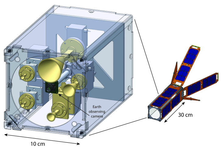
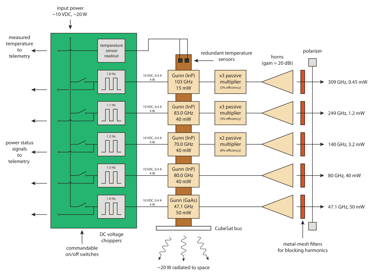
The calibration source in the payload consists of five amplitude modulated millimeter-wave “tones,” with one each at 47.1, 80.0, 140, 249 and 309 GHz. These five tones are designed to be well matched to (i) the observation windows in the atmospheric transmittance spectra, (ii) the Amateur Satellite Service bands in the Table of Frequency Allocations used by the Federal Communications Commission (FCC)444http://www.fcc.gov and The National Telecommunications and Information Administration (NTIA)555The United States Frequency Allocation Chart: http://www.ntia.doc.gov/files/ntia/publications/2003-allochrt.pdf, and (iii) the spectral bands commonly used in CMB polarimeters (more discussion in Section 5). A close-up view of the payload is shown in Figure 3. The 47.1 and 80.0 GHz tones are produced by Gunn diodes directly, while the 140, 249 and 309 GHz tones are produced by pairing a Gunn diode with a passive multiplier. The 140 GHz tone is created by a 70 GHz Gunn diode and a passive doubler, the 249 GHz tone is created by an 83 GHz Gunn diode and a passive tripler, and the 309 GHz tone is created by a 103 GHz Gunn diode and a passive tripler. Suitable Gunn diodes and multipliers are readily available from Spacek Labs and Virginia Diodes Inc. (VDI), respectively. The tones above 47.1 GHz are produced by InP Gunn diodes because they output more millimeter-wave power. This additional power is useful because the required multipliers have conversion efficiencies of only 3 to 8 %. The additional power is not needed at 47.1 GHz, so a lower-power-output GaAs Gunn diode is used for this tone. Each tone would have an associated conical horn antenna that would emit a coherent, linearly polarized beam because the input waveguide of the horn is rectangular and single-moded. A small amount of the unwanted cross-polarization, approximately -30 dB, is produced by the horns adding uncertainty to the orientation of the calibration source off axis. Therefore, a wire-grid polarizer666http://cosmology.ucsd.edu is installed at the payload aperture to suppresses this unwanted cross-polarization by an additional -30 dB or more for all five of the millimeter-wave sources. The final cross-polarization level is less than -60 dB, so 99.9999% of the power in the CalSat tones is emitted in a single polarization. The polarizer is installed with its transmission axis parallel to the co-polarization axis of the horn and slightly tilted to prevent standing waves between the horn and the polarizer. The millimeter-wave sources produce harmonics, so metal-mesh low-pass filters from QMC Instruments are mounted at the horn aperture of each source to eliminate any unwanted out-of-band radiation. It is important to emphasize that the CalSat tones are produced by commercially available components that are based on space-proven technologies, so the chance of a failure is comparatively low. Additional technical details are given in Table 2 and Figure 4. Alternative millimeter-wave sources such as broad waveguide-bandwidth noise sources were initially considered, but they are not compatible with the Table of Frequency Allocations used by the FCC and NTIA.
3.2.3 Ground Station
An S-band or UHF transmitter/receiver is used to communicate between the ground station and CalSat. Ground station hardware is commercially available from vendors like CubeSatShop777http://www.cubesatshop.com/ or Clyde Space888http://www.clyde-space.com/. This radio link is used for downloading data and uploading commands. The higher frequency S-band link provides a faster data rate and it is only used if more data bandwidth is necessary. Amateur UHF or S-band radio frequencies are available for CubeSats. The CalSat ground station includes a web server. Spacecraft attitude data and other data products and software libraries are distributed to the scientific community from this server.
3.3 Pre-launch Testing
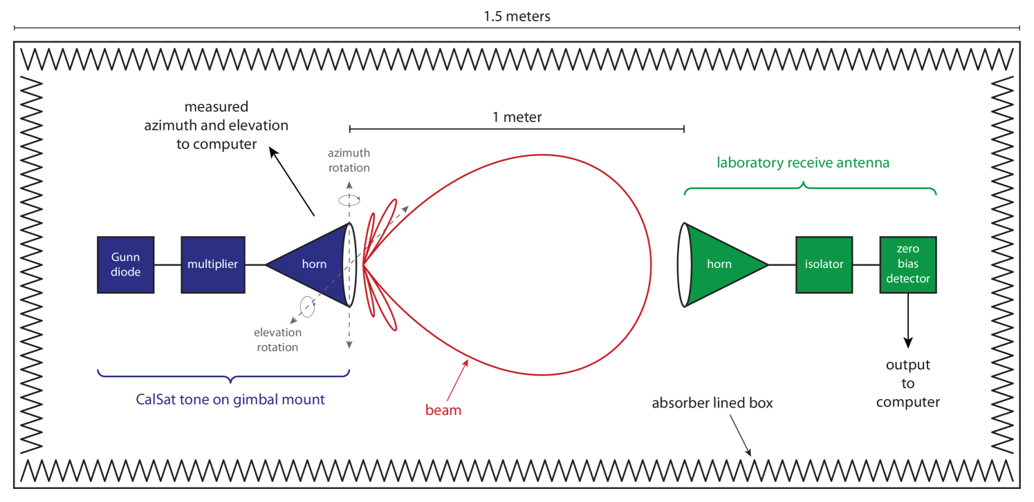
Prior to payload assembly, the horn beams are fully characterized, the source frequencies measured and the source beams mechanically aligned with the ADACS in the CalSat bus in the laboratory. The horn beams are mapped in two dimensions () with the antenna pattern measurement system shown in Figure 5. For this measurement, the CalSat millimeter-wave sources transmit power and are then pivoted about the phase center of the horn using a gimbal mount. A stationary receiver detects the emitted source power at each orientation. The gimbal mount is composed of two stepper-motor controlled rotation stages from Thor Labs. Both the co-pol and cross-pol beams are measured with this apparatus. The receiver in this system consists of a horn from Custom Microwave, a zero-bias Schottky diode detector from VDI and an isolator from Microwave Resources. The isolator inserted between the horn and the detector suppresses standing waves in the system. The beam mapping apparatus would need to be enclosed in a box lined with Eccosorb, which is a material that efficiently absorbs millimeter-waves Peterson & Richards [1984]; Halpern et al. [1986]. This baffle would ensure that reflected power does not produce spurious features in the beam map.
The millimeter-wave source frequencies are measured with a Fourier transform spectrometer (FTS). The receivers used in the beam mapping system are reused in this FTS measurement. This waveguide-bandwidth FTS measurement yields the precise frequency of each of the five tones with a very high signal-to-noise ratio. A second measurement is also done using the CalSat sources and a broadband 4 K bolometric receiver that can detect radiation below 650 GHz. For this second measurement, the source power is attenuated somewhat to match the dynamic range of the detector. This second measurement reveals any unwanted harmonics in the five tones, and it also shows that these harmonics are eliminated when the QMC Instruments filters are added.
The ADACS in the CalSat bus is designed to measure its own orientation to 0.05 deg. To ensure that the uncertainty in the polarization orientation of the CalSat tones is dominated by this ADACS pointing error the transmission axis of the polarizer in the payload must either be aligned to the ADACS reference system to better than 0.05 deg or the systematic offset angle between the two elements must be measured to better than 0.05 deg. Calculations show that aligning the polarizer to better than 0.05 deg would require micron precision, which should be achievable using standard precision metrology tools.
After CalSat is assembled, and the payload has been shown to work, the following required tests must be completed before launch: random vibration, sinusoidal vibration, shock, thermal vacuum cycle, thermal vacuum bake out, and a hardware configuration test. These tests are part of the CubeSat Program requirements and are defined by NASA’s Launch Services Program (LSP). A specialized spacecraft testing facility, such as the facility at Cal Poly, is required for these tests.
3.4 Launch, Orbit and Operations
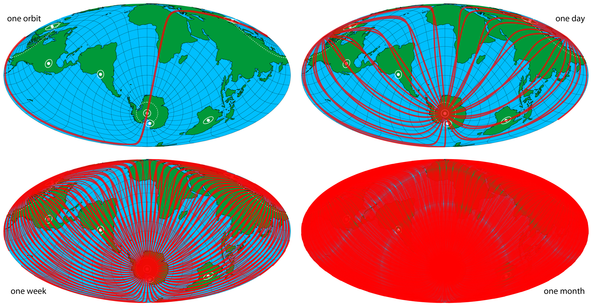
CalSat ideally will be placed in a polar orbit. A polar orbit is a particular type of low-Earth orbit (LEO) where a spacecraft travels in a north-south direction passing over both the north and south poles. Polar orbits are commonly used by Earth-observing satellites. While a spacecraft orbits in the north-south direction, the Earth moves beneath it in a west-east direction. If the precession rate of the orbit is phased appropriately, a satellite in a polar orbit will, over time, pass over the entire surface of the Earth. A conceptual diagram of this kind of orbit is shown in Figure 6. A polar orbit for CalSat ensures visibility from observatories in both the Northern Hemisphere, such as Mauna Kea in Hawaii and Summit Station in Greenland Asada et al. [2014], and the Southern Hemisphere, such as the Atacama Desert in Chile, and the South Pole. CalSat also will be observable by balloon-borne instruments flying from a range of locations, such as Ft. Sumner, New Mexico, Alice Springs, Australia and McMurdo Station in Antarctica. This global visibility makes CalSat the only source that can be observed by all terrestrial and sub-orbital millimeter-wave observatories. It is important to emphasize that a LEO does not have fixed Ra/dec coordinates on the sky, so CalSat would not permanently prevent a portion of the sky from being observed.
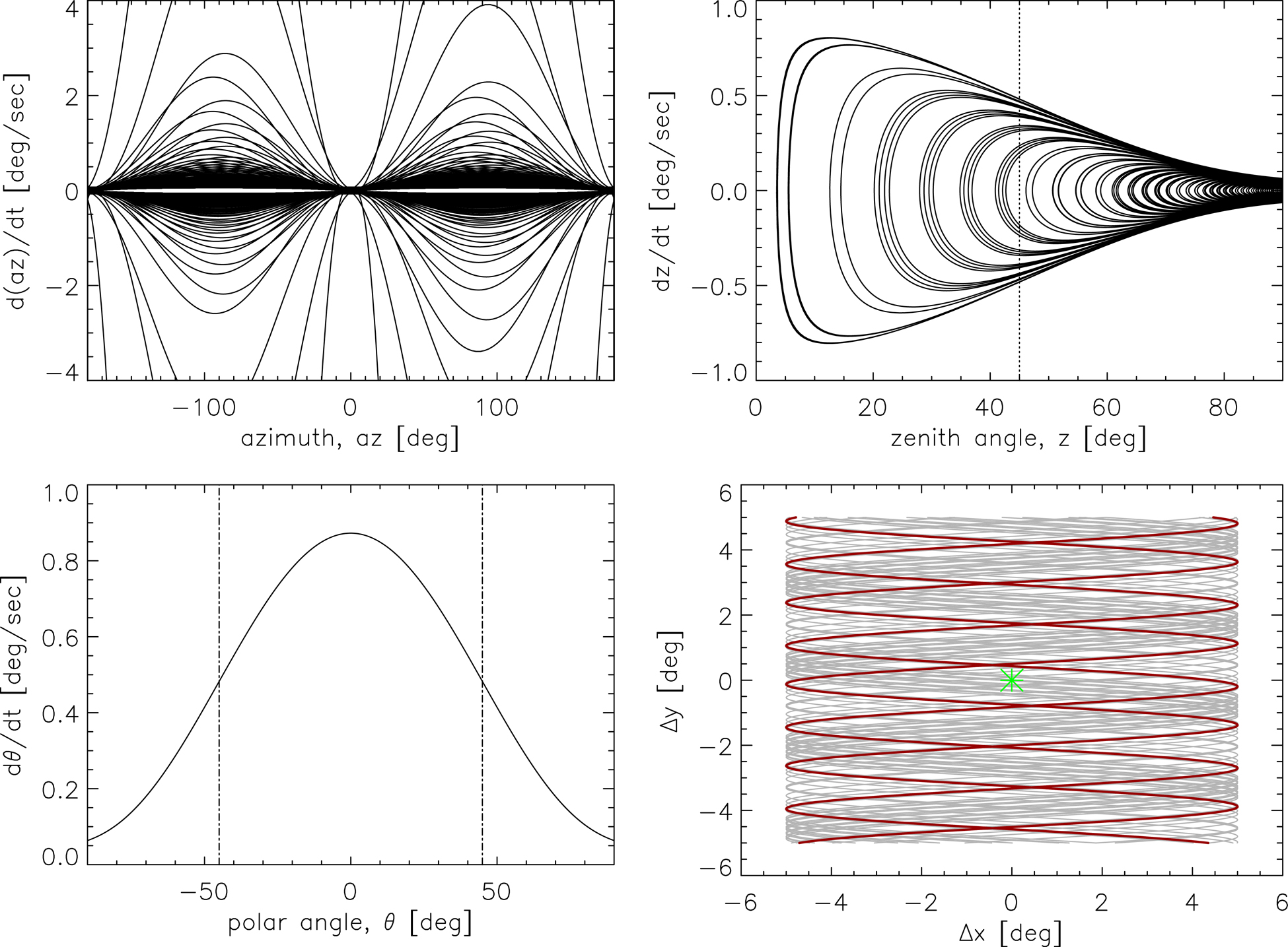
CalSat would be launched as an auxiliary payload on a DOD, NASA, or commercial rocket via launch programs such as NASA’s Educational Launch of Nanosatellites (ELaNa)999http://www.nasa.gov/offices/education/centers/kennedy/technology/elana_feature.html, NASA’s CubeSat Launch Initiative (CSLI)101010http://www.nasa.gov/directorates/heo/home/CubeSats_initiative.html or the Air Force’s University Nanosat Program (UNP)111111http://prs.afrl.kirtland.af.mil/UNP/. Because CalSat is launched as a flight of opportunity, the precise characteristics of the polar orbit, such as the altitude, can not be specified precisely before the launch opportunity is determined. Nevertheless, a target orbit is needed so the mission can be designed. We selected 500 km as the target altitude for the following three reasons. First, a 500 km orbit is achievable and viable. At approximately 1000 km the radiation environment substantially changes. Above 1000 km the Van Allen belts create a radiation environment that is too hostile for CubeSats. Below 1000 km the trace amount of atmosphere removes charged particles making the radiation density suitably low Larson & Wertz [1999]. Several existing CubeSats are in orbits with altitudes between 500 and 800 km. For comparison, the Hubble Space Telescope orbits at an altitude of 569 km. Second, at this altitude, air-drag becomes appreciable, and ultimately it can be used to de-orbit the CubeSat. Using the Drag Temperature Model (DTM) King-Hele [1987] we compute that the maximum expected lifetime of the CalSat orbit is approximately 16 years. This lifetime is compatible with the desired CalSat program, and it complies with the space debris guidelines established by the Inter-Agency Space Debris Coordination Committee (IADC) and the Office for Outer Space Affairs, which states that any CubeSat must de-orbit within 25 years of the end of its mission. Finally, performance forecasting studies show a 500 km altitude works well in terms of CalSat detectability (see Section 4). An altitude of 500 km corresponds to an orbital period of 1.6 hours, which means CalSat passes across the sky at the South Pole 14.2 times per day, and passes by other observatories several times per week (see Figure 7). The angular speed of CalSat varies with time as it passes by a given observatory. In Figure 8 we show the angular speed of CalSat as it passes by observatories at the South Pole and in the Atacama Desert in Chile. A typical CMB telescope should be able to track a source moving at these angular speeds.
The location of CalSat is tracked by the North American Aerospace Defense Command (NORAD) and quantified by a six element state vector that includes position and velocity information. NORAD would provide the state vector, which is uploaded to CalSat by the ground station. The ADACS would then use this state vector in conjunction with sensor information to determine the attitude of the spacecraft. The on-board computer would also take this position information, determine which observatory is closest, and then point the calibration beams at that observatory. During operation, the CalSat beams are pointed at CMB observatories using the ADACS and then modulated at approximately 1 Hz. By modulating the amplitude of the tones, it is easier to detect them if the beam-filling atmospheric emission is fluctuating. The calibration beam attitude is updated in real time as CalSat moves past the observatory to ensure the millimeter-wave source beams are fixed on that observatory. It is important to point out that the polarization orientation of the millimeter-wave sources is not fixed in Ra/dec, and it will slowly drift relative to the reference frame of the observer as CalSat moves across the sky. However, this polarization orientation drift is always measured to 0.05 deg using the on-board star cameras, so this effect can be precisely accounted for during data analysis in the same way orientation drift is treated with celestial sources.
The measured attitude is recorded as a function of time and this time-ordered data is telemetered to the ground station each orbit. The downloaded data would immediately be made publicly available via a web server. The measured source beam patterns (see Section 3.3) and CalSat attitude data would then be used by the CMB community in the analysis of their calibration measurements. End users of our data would need the azimuth, elevation, polarization orientation and the anticipated source brightness of CalSat as a function of time. To facilitate use of our data, the CalSat team would write a software library that would compute these needed quantities for any given latitude and longitude, and this software library is distributed along with the data.
| peak power [W] | duty cycle [%] | average power [W] | |
|---|---|---|---|
| payload | 20 | 20 | 4.0 |
| ADACS (MAI-400SS) | 2.2 | 100 | 2.2 |
| transceiver (Tx) | 5.5 | 10 | 0.55 |
| transceiver (Rx) | 0.25 | 100 | 0.25 |
| on-board computer | 2.0 | 100 | 2.0 |
| total | 30 | 9.0 |
3.5 Power Budget
A breakdown of the power budget for CalSat is given in Table 3. For the mission to be sustainable, the orbit average power (OAP) must be greater than the average power consumption. In this limit, the solar panels are able to, on average, both power the CubeSat and keep the on-board battery charged. Here we computed the OAP as the sun/eclipse ratio times the average available power from the solar panels during sunlight time, assuming the Earth’s albedo contribution is negligible during eclipse time. At 500 km, the sun/eclipse ratio is 0.62. Given the number of solar panels in the MISC3 CubeSat, the solar panel configuration (see Figure 2), and assuming each 3U panel can provide 2 W of power, we computed that between 13 and 24 W is available depending on the orbit angle. The average available power is 20 W during sunlight time, which means the OAP is 12 W. Table 3 shows that the average power consumption is conservatively 9 W, so the CalSat mission is sustainable with approximately 3 W of margin.
| Frequency | Aperture | ||||||
|---|---|---|---|---|---|---|---|
| [GHz] | [m] | South Pole | Chajnantor | Greenland | Mauna Kea | Ft. Sumner | McMurdo |
| 47.1 | 0.3 | 31 | 31 | 31 | 31 | 42 | 41 |
| 47.1 | 0.5 | 35 | 36 | 35 | 35 | 47 | 46 |
| 47.1 | 1.1 | 42 | 43 | 43 | 42 | 54 | 53 |
| 47.1 | 3 | 51 | 51 | 51 | 51 | ||
| 47.1 | 6 | 57 | 58 | 57 | 57 | ||
| 47.1 | 10 | 61 | 62 | 61 | 61 | ||
| 80.0 | 0.3 | 31 | 32 | 31 | 31 | 42 | 42 |
| 80.0 | 0.5 | 35 | 37 | 35 | 35 | 47 | 47 |
| 80.0 | 1.1 | 42 | 44 | 43 | 43 | 54 | 54 |
| 80.0 | 3 | 51 | 52 | 51 | 51 | ||
| 80.0 | 6 | 57 | 58 | 57 | 57 | ||
| 80.0 | 10 | 61 | 63 | 61 | 61 | ||
| 140 | 0.3 | 18 | 18 | 18 | 17 | 30 | 30 |
| 140 | 0.5 | 22 | 23 | 22 | 22 | 34 | 34 |
| 140 | 1.1 | 29 | 30 | 30 | 29 | 41 | 41 |
| 140 | 3 | 38 | 38 | 38 | 37 | ||
| 140 | 6 | 44 | 44 | 44 | 43 | ||
| 140 | 10 | 48 | 49 | 49 | 48 | ||
| 249 | 0.3 | 14 | 15 | 15 | 11 | 24 | 25 |
| 249 | 0.5 | 19 | 20 | 19 | 15 | 29 | 29 |
| 249 | 1.1 | 26 | 27 | 26 | 22 | 36 | 37 |
| 249 | 3 | 34 | 35 | 35 | 31 | ||
| 249 | 6 | 40 | 41 | 41 | 37 | ||
| 249 | 10 | 45 | 46 | 45 | 41 | ||
| 309 | 0.3 | 7 | 7 | 7 | 4 | 20 | 21 |
| 309 | 0.5 | 11 | 11 | 12 | 9 | 25 | 25 |
| 309 | 1.1 | 18 | 18 | 19 | 16 | 32 | 32 |
| 309 | 3 | 27 | 27 | 27 | 24 | ||
| 309 | 6 | 33 | 33 | 33 | 30 | ||
| 309 | 10 | 37 | 37 | 38 | 35 |
4 Detectability
For CalSat to be useful, the detected calibration signal needs to be large when compared with the noise level of the calibration measurement. It is difficult to forecast the precise characteristics of every instrument that might observe CalSat. Therefore, to assess the detectability, three primary assumptions were made. First, we assumed the aperture diameter of any instrument observing CalSat is between 0.3 and 10 m, which is the current range for CMB experiments. Second, we assumed A and . Here, is the aperture area, is the solid angle of the CMB telescope beam, and is the frequency of the incoming radiation with being the center frequency of the spectral band of the polarimeter. Third, we assumed the noise in the calibration measurement is dominated by photon noise from the CMB for balloon-borne measurements and the atmosphere for ground-based measurements.
To estimate the photon noise, spectral radiance curves were computed using the publicly available am atmospheric modeling software package121212The am software: https://www.cfa.harvard.edu/spaine/am/. We used am version 8.0, which implements O2 line mixing and non-resonant absorption near 60 GHz. Earlier versions of am did not model these effects, so these earlier versions had accuracy issues, which do not affect our calculations. The atmospheric profiles for the following six observatories were used in these simulations: South Pole, Chajnantor, Summit Station in Greenland, Mauna Kea, and balloon-borne observatories near Ft. Sumner, New Mexico, and McMurdo in Antarctica. For all sites, the zenith angle for observations was set to 45 deg. The altitude of the balloon-borne observatories was assumed to be 30 km. For the South Pole, Chajnantor, Greenland, and Mauna Kea observatories, the ambient temperature and PWV was assumed to be 230, 275, 248 and 275 K, and 1, 1, 1 and 4 mm, respectively. Given these conservative assumptions, the background power in the telescope beam and the associated photon noise equivalent power (NEP) were computed. The background power in the telescope beam was computed using
| (1) |
and the photon NEP was computed using
| (2) |
These equations are commonly used and their derivation can be found in the literature Lamarre [1986]; Richards [1994]. For our calculations, is the spectral radiance computed by am, is the spectral band-pass filter, which is a top-hat with a width equal to and A. We assumed observations are made with detectors that are sensitive to a single-polarization, so and . The results are shown in Figure 9 and Table 4. The expected millimeter-wave power from CalSat at the telescope aperture was computed using the following equation:
| (3) |
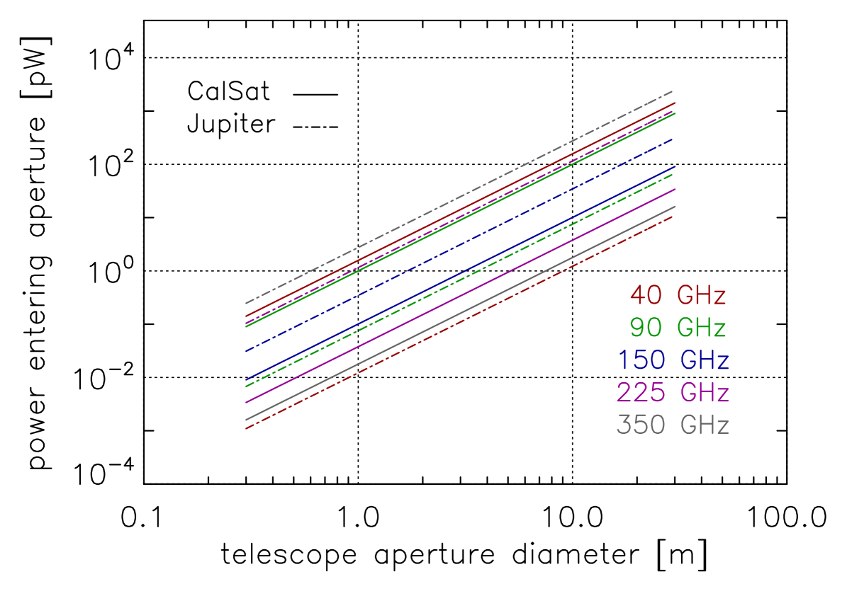
Here, is the millimeter-wave power from the source, is the horn gain in dBi, is the aperture diameter of the telescope, and is the distance between CalSat and the telescope; is the solid angle subtended by the telescope aperture as viewed from CalSat, and it is schematically shown in Figure 6. The power arriving in the telescope aperture from CalSat is plotted versus telescope aperture diameter in Figure 10. For comparison, the power arriving in the telescope aperture from Jupiter, which is a bright and commonly used unpolarized calibrator, was also computed and plotted alongside the CalSat curves in this Figure.
This analysis shows that (i) the brightness of CalSat is similar to the brightness of the background, (ii) the brightness of CalSat is comparable to Jupiter, and (iii) the signal-to-noise ratio for one second of integration is typically between 1,000 and 100,000. These are all characteristics of an ideal calibration source. If CalSat were significantly brighter than the background then the signal would likely saturate the detectors (assuming TES bolometers are being used, which is the current standard at these frequencies).
The CalSat instrument configuration presented in this paper was designed to support the following ongoing experiments and any associated follow-up experiments from these collaborations: ACT Naess et al. [2014], BICEP/KECK Ahmed et al. [2014]; Buder et al. [2014], CLASS Essinger-Hileman et al. [2014], GroundBIRD Tajiman et al. [2012], EBEX Reichborn-Kjennerud et al. [2010], PIPER Lazear et al. [2014], POLARBEAR Arnold et al. [2014]; Tomaru et al. [2012]; Kermish et al. [2012], QUIJOTE Perez-de-Taoro et al. [2014], SPIDER Rahlin et al. [2014], and SPTPol Benson et al. [2014]; Austerman et al. [2012]. Additional experiments that could use CalSat are being designed: GLP Araujo et al. [2014], SKIP Johnson et al. [2014], and QUBIC Ghribi et al. [2014]. And the planned CMB-S4 Abazajian et al. [2015b] program would benefit from CalSat because it could be used to both accurately calibrate deep observations and combine results from different observatories. Though CalSat is designed for CMB polarization experiments, it could also straightforwardly be used to calibrate other observatories such as ALMA and the VLA.
5 Discussion
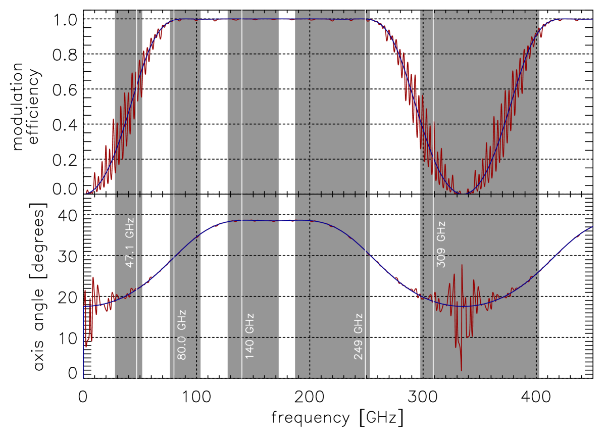
As a narrow-band source, CalSat is not designed to characterize the broad-band spectral properties of CMB polarimeters. Instead it is designed to provide the critical relationship between the coordinate system of the polarimeter in the instrument frame and the coordinate system on the sky that defines the astrophysical and Stokes parameters. The spectral bands in CMB polarimeters are typically broad, and some polarimeter technologies, such as the achromatic half-wave plate and the sinuous antenna multi-chroic pixel, have frequency dependent performance. Therefore polarimeter calibration must be performed over the full spectral bandwidth for experiments using these technologies. CMB experiment teams must characterize the spectral properties of their instruments in the laboratory before deployment and then use the clean and simple CalSat signals together with their lab-based instrument transfer functions during their calibration analyses. For example Figure 11 shows simulated modulation efficiency and polarimeter axis angle curves for an achromatic half-wave plate polarimeter. The 80.0, 140 and 249 GHz CalSat tones could be used to verify that the modulation efficiency is very close to unity at these frequencies and the polarimeter axis varies as expected as a function of frequency.
CalSat is programmed to listen for the ground station each orbit. If the radio uplink from the ground station fails, then the on-board computer turns the CalSat tones off and wait for the link to be restored. This mode of operation guards against out-of-control behavior. If this program malfunctions and the tones stay on, then the batteries will drain and the instrument will shutdown because the power budget can not support continuous operation. Therefore, the most likely failure mode is CalSat would turn off within 24 hours and then de-orbit 16 years later.
The selected tones match the Amateur Satellite Service Bands as stated in the text. We chose to use these bands because there is already an international agreement in place that allows instruments like CalSat to broadcast in these bands. It is possible to request permission to broadcast using other frequencies for a limited time by applying for an “experimental” license from the FCC131313FCC Public Notice DA:13-445. We avoided using this approach as a baseline plan because there is some risk involved. Projects using experimental licenses cannot cause interference and they cannot request protection from interference. The aforementioned Table of Frequency Allocations shows that below 300 GHz, all frequencies are already allocated, so interference is possible. Nevertheless, if CalSat moves forward, every effort will be made to maximize the utility of the instrument by adjusting the frequencies so they accommodate all possible users.
All experiments trying to extract cosmological information from the TB, EB and B-mode signals need a robust polarimeter calibration program that will allow the effect of instrument-induced errors to be mitigated during data analysis. A robust mitigation strategy for IPR, which is one of the most critical systematic errors, has not yet been identified because a suitable celestial calibration source does not exist and ground-based solutions are challenging. Moreover, the commonly used self-calibration technique, that uses the TB and EB spectra to remove any spurious B-mode signals, prohibits B-mode measurements from constraining the aforementioned isotropic departures from the standard model. CalSat was designed to be a low-cost, open-access solution to the IPR calibration problem for the CMB community, and its global visibility makes CalSat the only source that can be observed by all terrestrial and sub-orbital experiments. This global visibility makes CalSat a powerful universal standard that permits comparison between experiments from different observatories using appreciably different measurement approaches.
6 Acknowledgements
Johnson, Keating and Kaufman acknowledge support from winning a Buchalter Cosmology Prize (Second Prize) in 2014 for their paper entitled “Precision Tests of Parity Violation Over Cosmological Distances” Kaufman et al. [2014]. This paper explores the idea of using TB and EB spectra to study new physics via CPR, and these kinds of measurements rely on precise calibration enhancements; CalSat was used as an example of an enhanced calibration technique in this paper. We would like to thank Ari Buchalter and the Buchalter Cosmology Prize Advisory Board and Judging Panel for acknowledging our work with this prize.
References
- Abazajian et al. [2015a] Abazajian, K. N., et al. [2015a] Astroparticle Physics 63, 66–80.
- Abazajian et al. [2015b] Abazajian, K. N., et al. [2015b] Astroparticle Physics 63, 55-65.
- Adam et al. [2014] Adam, R., et al. [2014] A&A, submitted.
- Ahmed et al. [2014] Ahmed, Z., et al. [2014] Proc. SPIE 9153, 91531N.
- Araujo et al. [2014] Araujo, D., et al. [2014] Proc. SPIE 9153, 91530W.
- Arnold et al. [2014] Arnold, K., et al. [2014] Proc. SPIE 9153, 91531F.
- Asada et al. [2014] Asada, K., et al. [2014] Proc. SPIE 8444, 84441J.
- Aumont et al. [2010] Aumont, J., et al. [2010] A&A 510, A70.
- Austerman et al. [2012] Austermann, J. E., et al. [2012] Proc. SPIE 8452, 84521E.
- Baumann et al. [2009] Baumann, D., et al. [2009] AIP Conf. Proc. 1141, 10.
- Bennett et al. [2013] Bennett, C. L., et al. [2013] ApJS 208, 20B.
- Benson et al. [2014] Benson, B. A., et al. [2014] Proc. SPIE 9153, 91531P.
- BICEP2 Collaboration [2014a] BICEP2 Collaboration [2014] Phys. Rev. Lett. 112, 241101.
- BICEP2 Collaboration [2014b] BICEP2 Collaboration [2014] ApJ 792, 62.
- BICEP2/Keck and Planck Collaborations [2015] BICEP2/Keck and Planck Collaborations [2015] Phys. Rev. Lett. 114, 101301.
- Bock et al. [2006] Bock, J., et al. [2006] “Task Force on Cosmic Microwave Background Research.” (arXiv:astro-ph/0604101).
- Bock et al. [2009] Bock, J., et al. [2009] “Study of the Experimental Probe of Inflationary Cosmology (Epic)-Intemediate Mission for NASA’s Einstein Inflation Probe.” (astro-ph/0906.1188).
- Brown et al. [2009] Brown, M. L., et al. [2009] ApJ 705, 978.
- Buder et al. [2014] Buder, I., et al. [2014] Proc. SPIE 9153, 915312.
- Carroll et al. [1991] Carroll et al. [1991] Phys. Rev. D 43, 12.
- Crites et al. [2015] Crites et al. [2015] ApJ 805, 36.
- Essinger-Hileman et al. [2014] Essinger-Hileman, T., et al. [2014] Proc. SPIE 9153, 91531I.
- Ghribi et al. [2014] Ghribi, A., et al. [2014] Journal of Low-Temperature Physics 176, 5-6, 698-704.
- Gluscevic & Kamionkowski [2010] Gluscevic, V. and Kamionkowski, M. [2010] Phys. Rev. D 81, 12.
- Griffin et al. [1986] Griffin, M. J., et al. [1986] ICARUS 65, 244-256.
- Halpern et al. [1986] Halpern, M., et al. [1986] Applied Optics 25, 4.
- Johnson et al. [2014] Johnson, B. R., et al. [2014] Journal of Low-Temperature Physics 176, 5-6, 741-748.
- Keisler et al. [2015] Keisler, R., et al. [2015] ApJ 807, 151.
- Kamionkowski et al. [1997] Kamionkowski, M., Kosowsky, A. & Stebbins, A. [1997] Phys. Rev. D 55, 7368.
- Kaufman et al. [2014] Kaufman, J., Keating, B. G. & Johnson, B., R., [2015] MNRAS submitted arXiv:1409.8242.
- Keating et al. [2013] Keating, B. G., Shimon, M., & Yadav, A. P. S., [2013] ApJL 762, L23.
- Kermish et al. [2012] Kermish, Z., et al. [2012] Proc. SPIE 8452, 84521C.
- King-Hele [1987] King-Hele, D. G. [1987] Satellite Orbits in an Atmosphere: Theory and application, (Springer).
- Knox & Song [2002] Knox, L. & Song, Y. [2002] Phys. Rev. Let. 89, 011303.
- Lazear et al. [2014] Lazear, J., et al. [2014] Proc. SPIE 9153, 91531L.
- Lamarre [1986] Lamarre, J. M. [1986] Applied Optics 25, 6.
- Larson & Wertz [1999] Larson, W. J. & Wertz, J. R. [1999] Space Mission Analysis and Design (Third Edition), eds. Larson, W. J. & Wertz, J. R. (Microcosm).
- Naess et al. [2014] Naess et al. [2014] J. Cosmol. Astropart. Phys. 2014, 10.
- Ni [1977] Ni, W. [1977] Phys. Rev. Lett. 38, 7.
- O’Dea et al. [2007] O’Dea, D., Challinor, A., & Johnson, B. R. [2007] MNRAS 376, 1767.
- Perez-de-Taoro et al. [2014] Perez-de-Taoro, M. R., et al. [2014] Proc. SPIE 9145, 91454T.
- Peterson & Richards [1984] Peterson, J. B. & Richards, P. L. [1984] Int. J. Infrared Millimeter Waves 5, 1507.
- Planck Collaboration [2014] Planck Collaboration [2014] A&A 571, A1.
- Planck Collaboration [2015] Planck Collaboration [2015] A&A submitted arXiv:1507.02058v1.
- Pogosian et al. [2009] Pogosian, L., et al. [2009] JCAP 2, 13.
- POLARBEAR Collaboration [2014] The POLARBEAR Collaboration [2014] ApJ 794, 171.
- QUIET Collaboration [2011] QUIET Collaboration [2011] ApJ 741, 111.
- Rahlin et al. [2014] Rahlin, A. S., et al. [2014] Proc. SPIE 9153, 915313.
- Reichborn-Kjennerud et al. [2010] Reichborn-Kjennerud, B., et al. [2010] Proc. SPIE 7741, 77411C.
- Richards [1994] Richards, P. L. [1994] J. Appl. Phys. 76, 1.
- Savini et al. [2006] Savini, G., Pisano, G., & Ade, P. A. R. [2006] Applied Optics 45, 35.
- Smith et al. [2012] Smith, K. M., et al. [2012] JCAP 6, 14.
- Tajiman et al. [2012] Tajiman, O., et al. [2012] Proc. SPIE 8452, 84521M.
- Tomaru et al. [2012] Tomaru, T., et al. [2012] Proc. SPIE 8452, 84521H.
- Weiland et al. [2011] Weiland, J. L., et al. [2011] ApJS 192, 19.
- Yadav et al. [2012] Yadav, A., et al. [2012] Phys. Rev. D 86, 12.
- Zaldarriaga & Seljak [1997] Zaldarriaga, M. & Seljak, U. [1997] Phys. Rev. D 55, 4.