A data-driven MHD simulation of the 2011-02-15 coronal mass ejection from Active Region NOAA 11158
Abstract
We present a boundary data-driven magneto-hydrodynamic (MHD) simulation of the 2011-02-15 coronal mass ejection (CME) event of Active Region (AR) NOAA 11158. The simulation is driven at the lower boundary with an electric field derived from the normal magnetic field and the vertical electric current measured from the Solar Dynamics Observatory (SDO) Helioseismic Magnetic Imager (HMI) vector magnetograms. The simulation shows the build up of a pre-eruption coronal magnetic field that is close to the nonlinear force-free field (NLFFF) extrapolation, and it subsequently develops multiple eruptions. The sheared/twisted field lines of the pre-eruption magnetic field show qualitative agreement with the brightening loops in the SDO Atmospheric Imaging Assembly (AIA) hot passband images. We find that the eruption is initiated by the tether-cutting reconnection in a highly sheared field above the central polarity inversion line (PIL) and a magnetic flux rope with dipped field lines forms during the eruption. The modeled erupting magnetic field evolves to develop a complex structure containing two distinct flux ropes and produces an outgoing double-shell feature consistent with the Solar TErrestrial RElations Observatory B / Extreme UltraViolet Imager (STEREO-B/EUVI) observation of the CME. The foot points of the erupting field lines are found to correspond well with the dimming regions seen in the SDO/AIA observation of the event. These agreements suggest that the derived electric field is a promising way to drive MHD simulations to establish the realistic pre-eruption coronal field based on the observed vertical electric current and model its subsequent dynamic eruption.
1 Introduction
Large scale solar eruptions such as solar flares and coronal mass ejections are major drivers of space weather near Earth (e.g. review by Temmer, 2021). These eruptive phenomena are all manifestations of the explosive release of magnetic energy stored in the non-potential, current carrying coronal magnetic fields built up over time due to magnetic flux emergence from the interior and shear and twisting motions at the interior footpoints of the coronal field lines (e.g. Forbes et al., 2006; Green et al., 2018; Patsourakos et al., 2020). Thus determining the realistic 3D coronal magnetic field evolution of the solar eruptive events is essential to understanding the physical mechanisms that have led to the eruptions and also advancing the capability of predicting their space weather impact. In recent years, simulations using observed data for constructing the initial and boundary conditions, called “data-constrained” and “data-driven” simulations, have undergone significant development and been applied to study real solar eruptive events with complex magnetic structures (see e.g. recent review by Jiang et al., 2022). For example, these approaches have been extensively explored to model the magnetic field evolution of the X2.2 flare and the associated halo CME on 2011–02-15 from Active Region (AR) NOAA 11158 (e.g. Cheung & DeRosa, 2012; Inoue et al., 2014, 2015; Hayashi et al., 2018; Hoeksema et al., 2020; Afanasyev et al., 2023), which is a well observed quadrupolar, -sunspot active region.
Cheung & DeRosa (2012) and Hoeksema et al. (2020) have developed a frame work of boundary data-driven magneto-frictional (MF) modeling of the force-free coronal magnetic field evolution of AR 11158, using an electric field inverted from the HMI vector magnetograms (Kazachenko et al., 2014; Fisher et al., 2020) as the lower boundary driving condition. They are able to model the quasi-static build up of the active region magnetic field on realistic time scales, but cannot model the dynamic eruption phase with the MF approach. Inoue et al. (2014) and Inoue et al. (2015) used a NLFFF extrapolation at about 2 hours before the onset of the eruptive flare of AR 11158 as the initial state and modeled the subsequent dynamic eruption with the zero- MHD simulation. It is found that the twisted field of the initial NLFFF is stable and that strongly twisted field lines are formed via the tether-cutting reconnection, which is responsible for the onset of the eruption. Afanasyev et al. (2023) used a hybrid approach where the build up of the active region is modeled with the data-driven MF simulation and a snapshot from the MF simulation at a time about 1.5 hours before the onset of the eruption is used as the initial magnetic field configuration for the MHD simulation to model the subsequent dynamic eruption. It is found that the initial magnetic field is already out of equilibrium and erupts immediately while at the same time also going through an initial relaxation, so it is difficult for the simulation to assess the initiation mechanism of the eruption. Thus a data-driven MHD simulation that models both the quasi-static build up and transition to dynamic eruption is needed to examine the initiation mechanisms. However it is still not feasible for such MHD simulations to model the long build up phase of the active region on realistic time scales. Hayashi et al. (2018) has developed a data-driven MHD simulation of AR 11158 driven with a lower boundary electric field inverted from the temporal evolution of the three components of the vector magnetic field from the HMI vector magnetograms. Applying this electric field on an accelerated time scale, their MHD simulation was able to reproduce the observed temporal evolution of the (smoothed) photospheric magnetic field at the lower boundary and build up a pre-eruption coronal magnetic field with sufficient free magnetic energy to drive the X-class flare, but did not result in the release of the magnetic energy and the development of the eruption.
In this work, we use a new electric field derived from the observed normal magnetic field and vertical electric current evolution from the SDO/HMI vector magnetograms for the lower boundary driving of an MHD simulation of the eruptive flare and CME developed from AR 11158 on Feb. 15, 2011. The preliminary results of the simulation were reported in a NASA Living With a Star focused science team joint paper (section 4 of Linton et al., 2023). Here we present a more detailed description of the simulation and the results, and expand on the analysis of the erupting magnetic field and comparison with the observations by the STEREO-B EUVI and the SDO/AIA. We found the build up of a pre-eruption magnetic field that is close to the NLFFF extrapolation and the onset of the subsequent eruption that reproduces some of the observed features of the CME by the STEREO-B EUVI and the SDO/AIA. The paper is organized as follows. In §2 we describe the setup of the MHD simulation and the formulation of the lower boundary driving electric field. In §3 we present the simulation results and comparison with the observations. The conclusions and a discussion are given in §4
2 Description of the data-driven simulation
An earlier description of the setup of the simulation was given in section 4 of Linton et al. (2023) which reported preliminary results of the simulation. Here for the completeness of this paper, we provide a more detailed description of the simulation setup and the lower boundary driving electric field used.
2.1 The numerical model
The data-driven simulation is carried out using the “Magnetic Flux Eruption” (MFE) code which solves the set of semi-relativistic MHD equations as described in Fan (2017, hereafter F17). The readers are referred to that paper for a description of the equations solved and the numerical methods. Here we only describe the changes made specifically for the setup of the current simulation.
As described in F17, the momentum equation includes the Boris correction with a reduced speed of light to limit the Lorentz force, and hence relax the stringent Courant condition on the numerical time-stepping due to the extremely high Alfvén speed present in the simulation domain which contains a strong active region. For this simulation, we have used a reduced speed of light of about km/s, which remains significantly higher than the peak plasma flow speed and the the sound speed reached in the simulation. For the thermodynamics, we assume an ideal gas of fully ionized hydrogen, with , and solve the internal energy equation taking into account the following non-adiabatic effects that include the field aligned thermal conduction, optically thin radiative cooling, and coronal heating. However, we no longer include an empirical coronal heating (eq. (14) in Fan, 2017) for the heating term in the internal energy equation (term H in eq. (5) of Fan, 2017), but only include the resistive and viscous dissipation due to the numerical diffusion (as described on p.3 of Fan, 2017). For this simulation, we add to the lower boundary a random electric field (as described below in §2.2) representing the effect of turbulent convection that drives field line braiding, and the resultant (numerical) resistive and viscous heating provides the heating of the corona. This heating varies spatially and temporally self-consistently with the formation of the strong current layers in the 3D magnetic field.
The simulation is carried out in a spherical wedge domain whose lower boundary is centered on and tracked the active region. Figure 1 shows the simulation domain against the solar disk as viewed from the Earth perspective on 2011-02-15 at 02:00:00 UT.
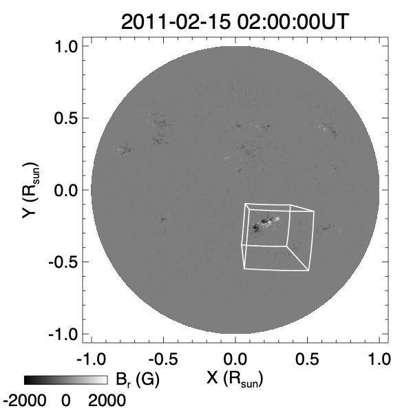
It has a latitudinal width of 17.2 degrees, a longitudinal width of 18.8 degrees, and a radial range of 1 to 1.43 solar radius. The simulation domain is resolved with a grid of . The grid is stretched in the radial dimension (with the radial grid size increasing outward as a geometric series) and is uniform in the two horizontal dimensions. The peak radial resolution is 300 km at the bottom, and the horizontal resolution is 724 km at the bottom.
2.2 Formulation of the lower boundary electric field
For the lower boundary magnetic flux transport driving conditions, we impose a time dependent horizontal electric field that consists of three components:
| (1) |
The first component corresponds to the horizontal component of the so-called “PTD” (Poloidal-Toroidal-Decomposition) electric field derived in Fisher et al. (2020, see the horizontal component of eq. (8) in that paper):
| (2) |
where is computed from the observed normal magnetic field () evolution on the photosphere by solving the 2D Poisson equation (eq. (9) in Fisher et al., 2020):
| (3) |
due to Faraday’s law. Imposing reproduces the observed photospheric normal magnetic field evolution on the lower boundary.
The second term on the right hand side of equation (1) is the “twisting” electric field. It is given as the horizontal gradient of a potential:
| (4) |
such that it does not alter the observed evolution (already reproduced by imposing the component), and we assume that it corresponds to a vertical transport of a horizontal magnetic field into the domain, i.e.
| (5) |
where is the vertical transport speed, which we assume to be a constant, and is a horizontal magnetic field, which we note is not the same as the observed horizontal field and it can be shown from equation (5) that (which condition is generally not satisfied by the observed horizontal magnetic field). Further taking the horizontal divergence of equation (5) yields:
| (6) |
We let be equal to , which is the vertical electric current derived from the observed horizontal magnetic field in the photospheric vector magnetograms. Thus we have
| (7) |
We compute the potential by solving the 2D Poisson equation (7) given the measured vertical electric current at the photosphere from the HMI vector magnetograms and specifying , which is an ad hoc parameter we can adjust. For the simulation presented here we have used , which is small enough to ensure a quasi-static evolution for the build-up phase but high enough to compete with numerical diffusion to produce the eruptive behavior close to that observed. Once is determined, the twisting electric field is given by equation (4). Imposing at the lower boundary corresponds to transporting a (divergence-free) horizontal magnetic field () with the observed vertical electric current into the domain, without changing the normal magnetic field evolution at the lower boundary. It effectively transports twist into the corona based on the observed vertical electric current.
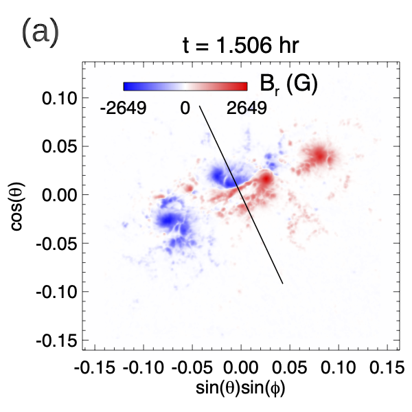
Figure 2 shows example snapshots of the observed normal magnetic field , the vertical electric current density , and the horizontal twisting electric field components and derived based on (from eqs. [4] and [7]), at the time of about 1.9 hour before the onset of the observed X-class flare.
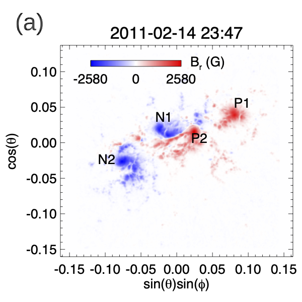
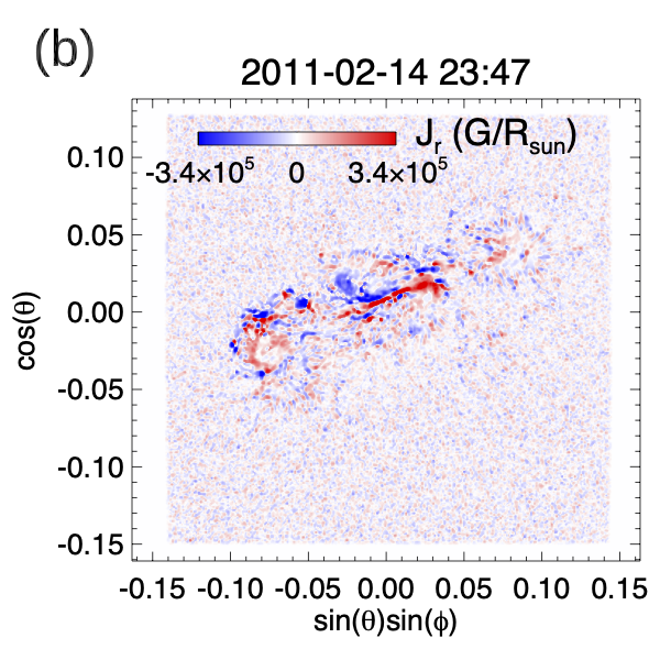
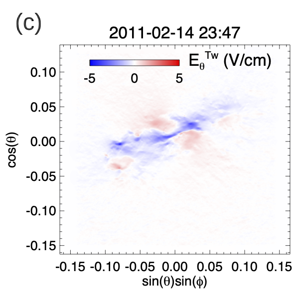
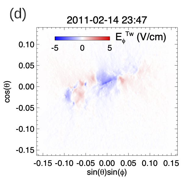
From panels (a) and (b) we can see that significant which tends to be of the same sign as is present in the polarity concentrations P2 and N1 near the central polarity inversion line (PIL). On the other hand, in the polarity concentration N2, we find of predominantly opposite sign of . As a result, the derived twisting electric field (panels (c) and (d)) transports positive twist into the corona at the central P2, N1 flux concentrations and negative twist at the N2 flux concentration. It can be seen from panels (c) and (d) that , and transport a concentrated horizontal, shear magnetic field component into the corona at the central PIL. They also effectively drive a clockwise rotation of the P2 and N1 flux concentrations and a counter-clockwise rotation of the N2 flux concentration.
We note that Cheung & DeRosa (2012) have also used a horizontal electric field to drive twist into the corona in their magneto-frictional modeling of the evolution of AR 11158. In that case, effectively a uniform rotation of all the polarity concentrations is applied to drive the same sign of twist into the corona. Here with the twisting electric field, the twist injection varies spatially based on the distribution of the observed vertical electric current.
The last term on the right hand side of equation (1) is a random, horizontal electric field given by (see e.g. Fan, 2022):
| (8) |
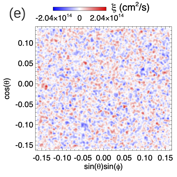
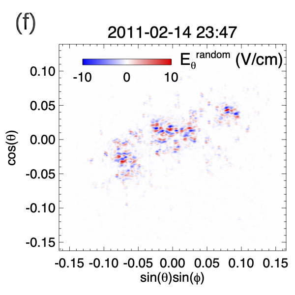
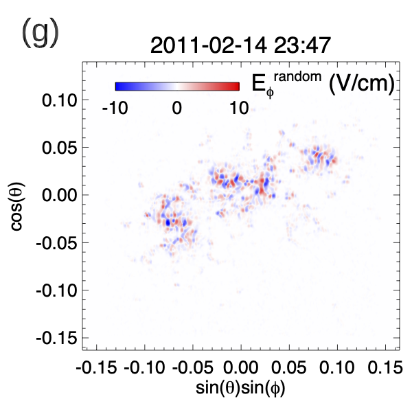
Again, this is given as the gradient of a scalar field and thus does not alter the observed on the lower boundary (reproduced by imposing ). The formulation of this electric field is inspired by that of the “STatistical InjecTion of Condensed Helicity” (“STITCH”) electric field (Mackay et al., 2014; Dahlin et al., 2022) used for modeling helicity condensation and filament channel formation. But here, used in equation (8) is a time dependent field that is made up of a superposition of 15721 randomly placed cells of opposite sign values. Each cell has a 2D Gaussian profile with a size scale of 1.74 Mm and a peak amplitude of , and varies temporally as a sinusoidal function with a period and life time of 11.89 min. Figure 2(e) shows a snapshot of the field, which illustrates its random cellular pattern, and the resulting random electric field components (Figure 2(f)), and (Figure 2(g)) produced at the lower boundary when this field and the given in Figure 2(a) are applied in equation (8). As is described in Fan (2022), effectively drives random rotations of the foot points of the flux concentrations, with positive (negative) corresponding to clockwise (counter-clockwise) rotation. Here the positive and negative signed cells in the field are statistically balanced, therefore no net twist or helicity is driven into the corona by . It represents the effect of turbulent convection that drives field-line braiding which produces resistive and viscous heating in the corona. Similar ways of driving coronal heating by imposing random foot-point motions that represent turbulent convection at the photospheric lower boundary of MHD simulations have been widely used (e.g. Gudiksen & Nordlund, 2005; Warnecke & Peter, 2019).
Even though the driving electric field is derived from the photosphere magnetograms, we impose a fixed chromosphere temperature of 20,000 K and density of at the lower boundary. The boundary conditions for the side and top boundaries in the present simulation are the same as those used in Fan (2017).
2.3 The initial state
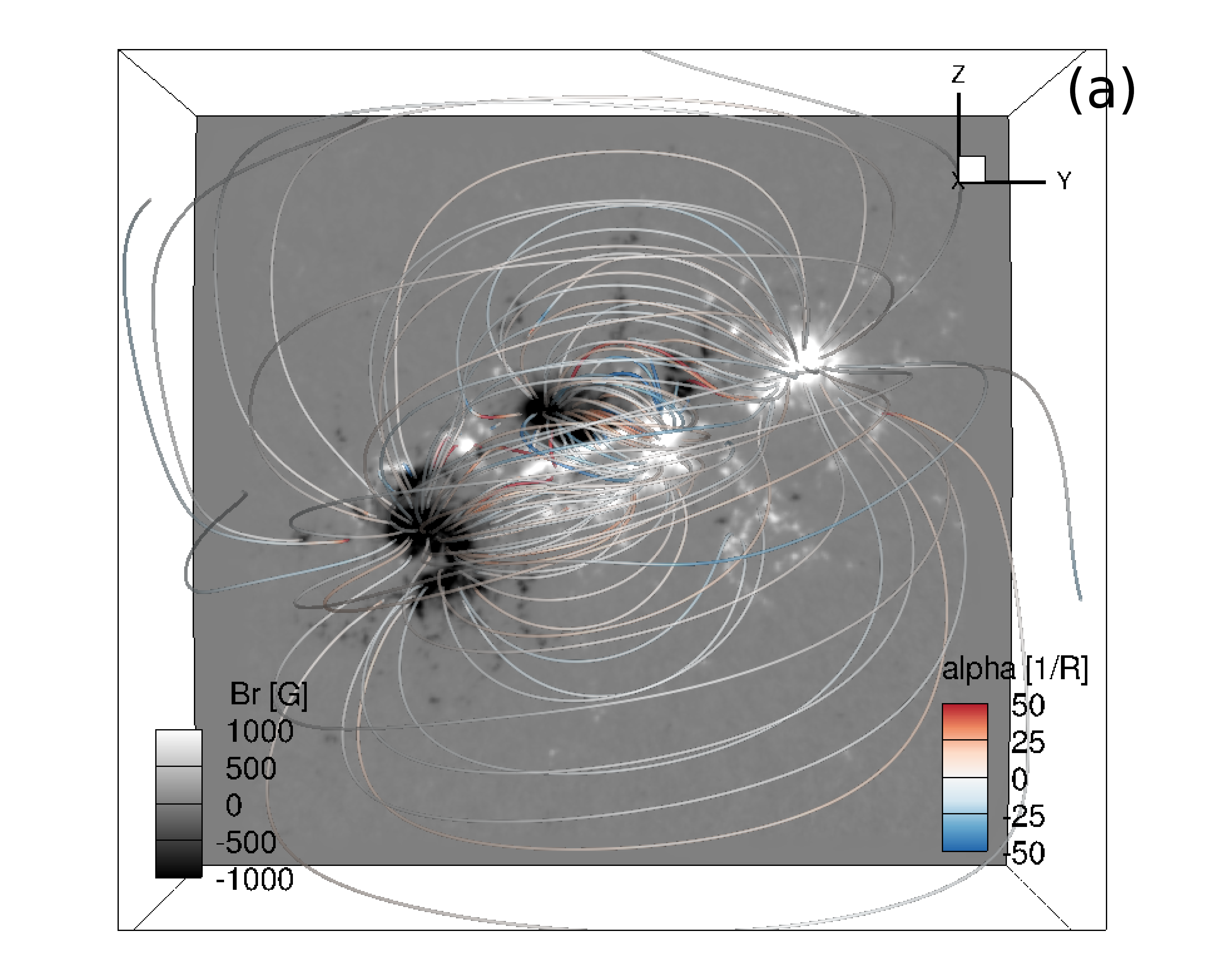
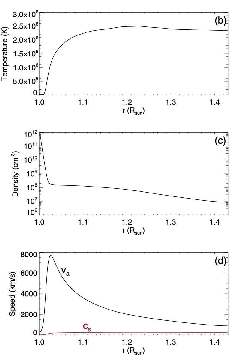
To set up the initial state of the data-driven simulation, we start with a potential magnetic field extrapolated from the observed photospheric normal magnetic field at 2011-02-14 23:47 UT (Fig. 2(a), about 1.9 hours before the onset of the observed X-class flare), and numerically evolve the MHD state by driving at the lower boundary with only the random electric field until it reaches a quasi-steady state with a hot corona. Figure 3 shows the 3D magnetic field lines (panel (a)) colored with the twist rate defined as where is the current density, and the radial profiles of the horizontally averaged temperature (panel (b)), density (panel (c)), and the Alfvén and sound speeds (panel (d)) of the relaxed, quasi-steady state reached. It can be seen that the magnetic field (panel (a)) for the relaxed state is no longer the potential field but contains some random twist due to the driving random electric field (which does not drive a net helicity into the domain), although most field lines remain near zero (white color), and the magnetic energy remains very close to that of the potential field energy (being about 1.0016 of the potential field energy). A quasi-steady atmosphere with a reasonable temperature and density stratification (panels (b) and (c)) that contains a chromosphere transitioning into a hot corona is established. The Alfvén speed is significantly higher than the sound speed throughout the domain (panel (d)).
We then use this relaxed state as the initial state (defined hereafter as ) for the simulation, driven at the lower boundary with all three electric fields given in the right hand side of equation (1) (derived from a time sequence of the vector magnetograms starting from 2011-02-14 23:47 UT) for a perid of over 2.8 hours. The following section describes the resulting evolution obtained from the boundary data-driven simulation.
3 Simulation results
3.1 Overview of evolution
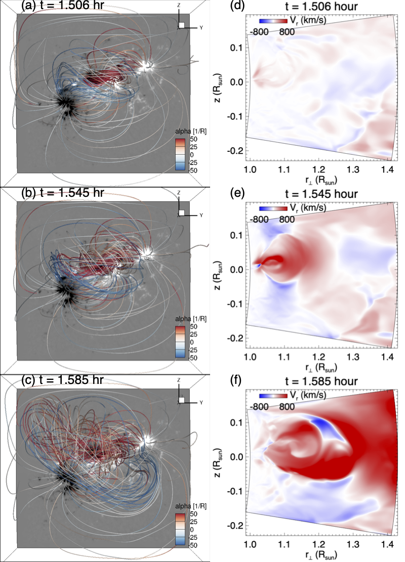
Figure 4 shows the resulting evolution of the 3D magnetic field (left column images), the radial velocity in the central meridional cross-section (middle column), and several integrated quantities (right column) that include the free magnetic energy (panel (g)), which is the excess of the total magnetic energy over that of the corresponding potential magnetic field, the total kinetic energy (panel (h)), and the various contributions to the rate of change of the total magnetic energy (panel (i)) which are described in the following.
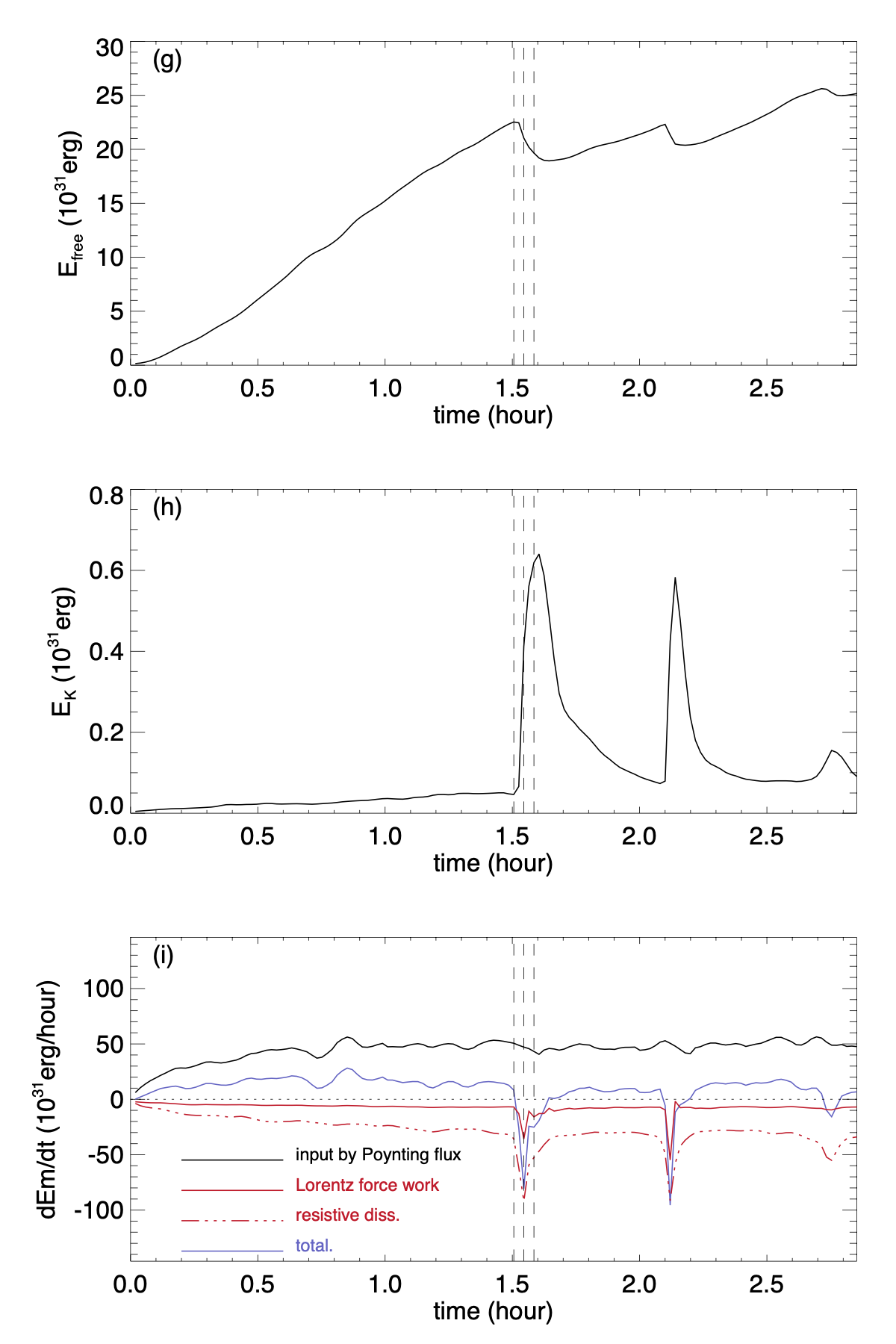
(1) The black curve in panel (i) shows the input of magnetic energy by the Poynting flux integrated over the lower and upper boundaries: , where is the radial component of the Poynting flux density and the integration is over the area of the lower and upper boundaries (note no Poynting flux through the side boundaries due to the conducting wall side boundary condition). (2) The solid red curve shows the release of magnetic energy resulting from the Lorentz force work: , where is the Lorentz force, is the velocity, and the integration is over the volume of the domain. (3) The red dash-dotted curve shows the dissipation of magnetic energy by the numerical magnetic diffusion: , where is the electric field resulting from the numerical diffusion evaluated in the numerical code. The blue curve shows the sum of the above three, which is the net rate of change of the total magnetic energy. We see an overall continuous build up of the free magnetic energy (panel (g)) due to the continuous Poynting flux input (black curve in panel (i)) at the lower boundary produced by the driving electric field ( given by eq. [1]). This Poynting flux input is in excess of the dissipations of the magnetic energy due to the resistive dissipation (red dash-dotted curve in panel (i)) and the Lorentz force work (red solid curve in panel (i) ), resulting in a continuous net gain of the free magnetic energy (blue curve in panel (i)) for most of the time. But this continuous build up is punctuated by sudden free magnetic energy releases and kinetic energy increases (at about hour, hour, and hour), due to the sudden enhancements of the Lorentz force work and resistive dissipation resulting from the loss of equilibrium of the magnetic field (see the movie for the whole course of the evolution).
During the first 1.5 hour period, increases steadily, while and the Lorentz force work remain small with the magnetic field being in quasi-equilibrium. We can see from the movie of Figure 4 that during this time the magnetic field is being sheared and twisted as indicated by the color of the field lines, forming positive-twisted (red field lines) sigmoidal shaped loops above the central (PIL) and negative-twisted (blue field lines) inverse-S shaped loops connecting to the following negative polarity sunspot (panel (a)). At about hour, the free magnetic energy reaches a peak value of about (panel (g)), and then we see the onset of the first eruption with a sudden outward acceleration of the central sigmoid field (panels (b) and (e)), forming a positive-twisted erupting flux rope (red twisted field lines) which also pushes out and accelerates an outer negative-twisted field (blue field lines) (panels (c) and (f) and the movie).
3.2 The Pre-eruption Magnetic Field
Figure 5 shows the pre-eruption magnetic field just before the onset of the eruption at hour. The top two panels show a set of 3D magnetic field lines colored with the current density (panel (a)) and the twist rate (panel (b)).
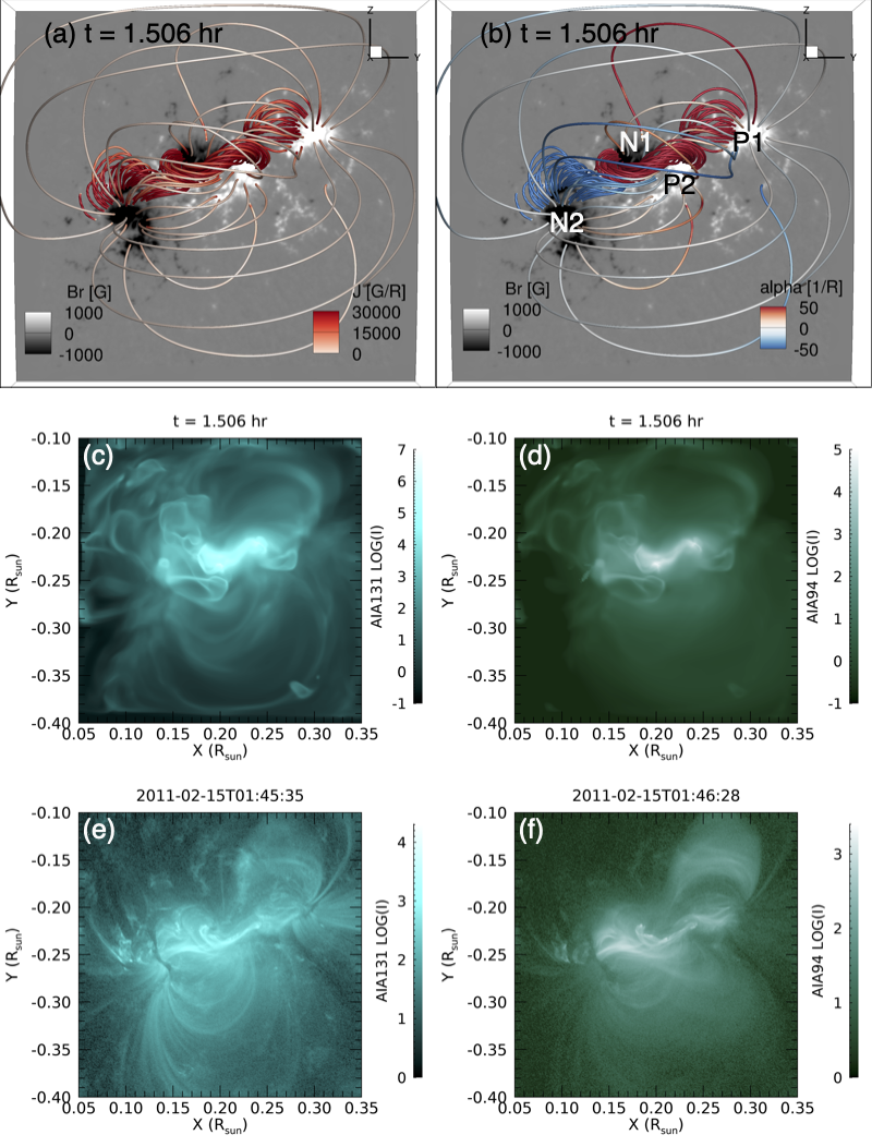
Comparing the pre-eruption field in Figure 5(b) to the nearly potential field of the initial state in Figure 3(a), we find that the twisting electric field has built up highly sheared, forward S-shaped (sigmoid) loops with positive (right-handed) twist rates above the central PIL connecting polarities P2, N1, and also positive-twisted loops connecting polarities P1, N1. Furthermore, we find negative-twisted (left-hand-twisted) loops (blue with negative ) connecting P2, N2 polarities, and some higher loops with negative twist connecting P1, N2 polarities. As pointed out earlier in Figure 2, the twisting electric field imposed in N2 (with opposite signs of and ) transports negative twist into the corona, opposite to the twisting electric field dominating in the other polarity concentrations that drives positive twist into the corona.
It can be seen in Figure 5(a) that the field lines with the strongest current density show morphology in qualitative agreement with the brightening loops in the observed hot channel images of SDO/AIA (Figs. 5(e) and 5(f)). This indicates that the model captures the structure of the non-potential (energized) magnetic field. Figures 5(c) and 5(d) show respectively the synthetic AIA 131 Å and 94 Å images at the same time of the pre-eruption magnetic field shown in Figures 5(a) and 5(b). The synthetic images are computed by integrating along the line of sight (from the Earth perspective) through the simulation domain:
| (9) |
where denotes the length along the line of sight through the simulation domain, denotes the intensity at each pixel in units of DN/s/pixel (shown in LOG scale in the images), is the electron number density, and is the temperature response function of the corresponding AIA filter (obtained by running the SolarSoft routine get_aia_response.pro). The synthetic AIA images (Figs. 5(c) and 5(d)) also show some qualitatively similar emission features as those in the observed ones (Figs. 5(e) and 5(f)), i.e. the central forward S-shaped sigmoid emission along the central PIL, and the surrounding large loops connecting the major polarity concentrations. We find that the central sigmoid emission is due to the heating produced by the formation of a strong current layer in the strongly sheared field above the central PIL.
To examine how close to force-free the pre-eruption magnetic field is, we have evaluated , the current-weighted mean of the sine of the angle between the current density and the magnetic field (Wheatland et al., 2000):
| (10) |
where
| (11) |
the subscript “i” denotes each grid point and the sum is over all the grid points in the simulation domain. We found , corresponding to a (current-weighted) mean angle of about between the current density and the magnetic field vectors, i.e. close to being force-free. Furthermore we found that the vertical current density obtained at the simulation lower boundary is close to the observed from the HMI vector magnetogram at the corresponding time, for the large-scale main current patches, as can be seen in Figure 6 (compare panels (b) and (c)).
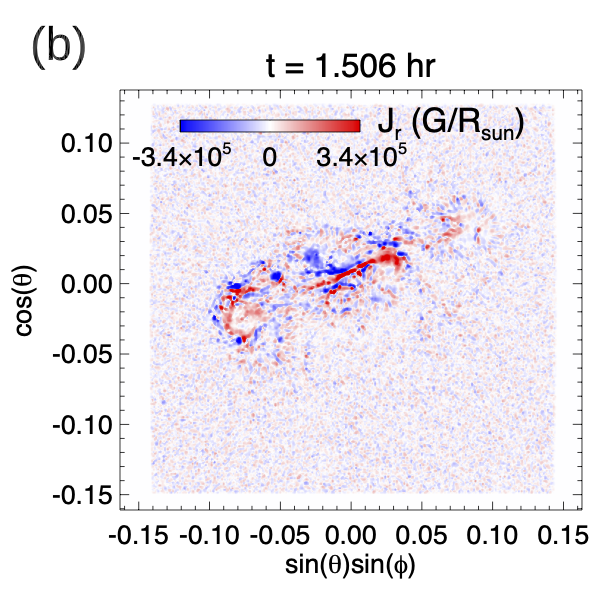
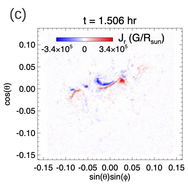
This shows that the modeled pre-eruption magnetic field is close to the solution of a NLFFF extrapolation from the observed vector magnetogram. Indeed, the peak free energy of the pre-eruption magnetic field reached just before the first eruption () is close to the result obtained in Sun et al. (2012), who carried out the NLFFF extrapolation of the coronal magnetic field of AR 11158 and found that the free magnetic energy reaches a maximum of just befored the onset of the observed X2.2 flare. As described in §2.2, the twisting electric field we impose does not enforce the observed horizontal magnetic field at the lower boundary. Nevertheless, we find that the resulting horizontal magnetic field at the lower boundary for the pre-eruption magnetic field that is built up is very similar to that of the observed.
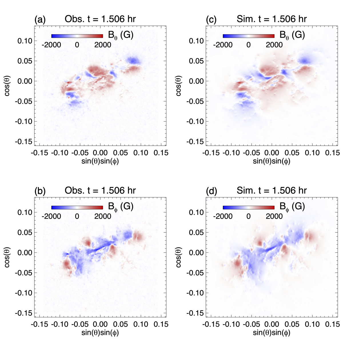
Figure 7 shows a comparison of the horizontal components of the magnetic field at the lower boundary at the onset of the simulated eruption with those from the photospheric vector magnetogram at the same time. We see very similar patterns for both the and components comared to the observed ones.
3.3 The initiation of eruption
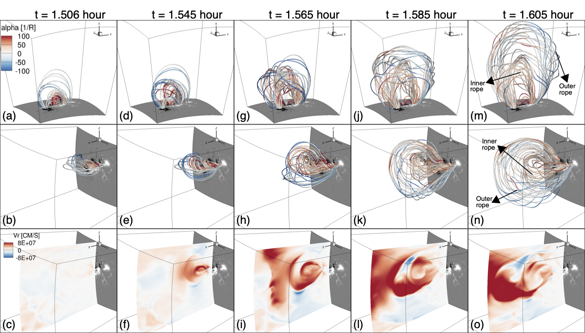
Figure 8 shows the 3D evolution of a set of erupting magnetic field lines as viewed from 2 different perspectives (top 2 rows) during the first eruption. The field lines are traced from a set of Lagrangian tracer points tracked in the velocity field. The eruption begins with the acceleration of the highly sheared sigmoid field with positive twist above the central PIL (see the red field lines in panel (a) and the sudden onset of the rise velocity from panel (c) to panel (f) of Fig. 8). To examine what might have triggered the sudden acceleration of the sigmoid field above the central PIL and whether it contains a magnetic flux rope, we plotted in Figure 9 the distribution of twist rate and the radial curvature in the vertical cross-section, whose location is indicated by the black line across the central PIL in Figure 6(a), at the time of the onset of the eruption ( hour, top row) and at a time during the eruption( hour, bottom row).
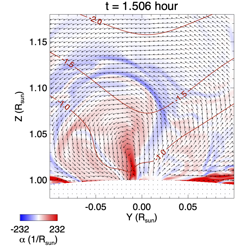
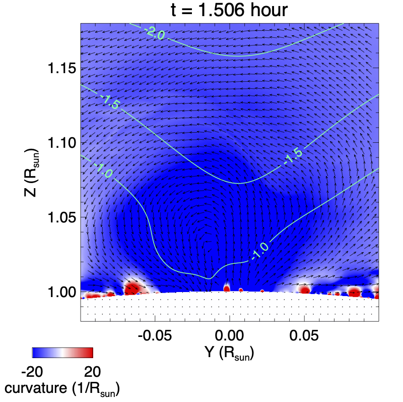
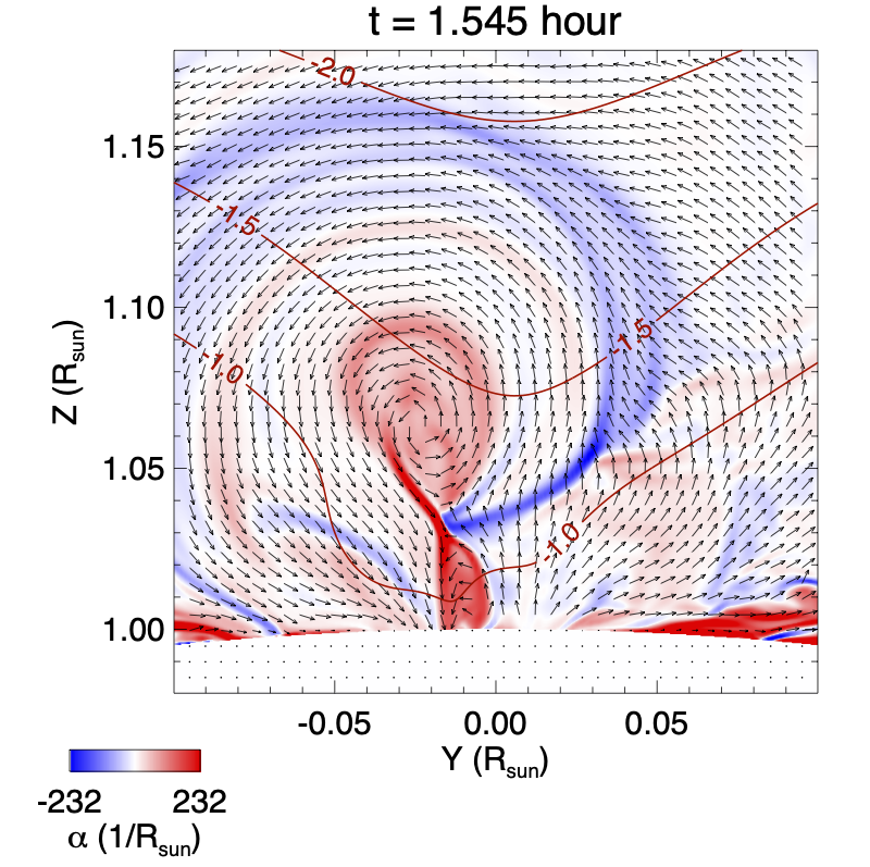
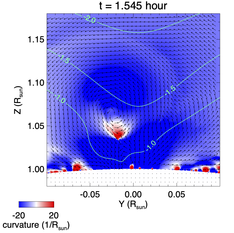
It can be seen in the top left panel that most of the current of the positive-twisted (red) sigmoid field region is still below the contour of the critical decay index of for the onset of the torus instability (e.g. Kliem & Török, 2006). Here is the horizontal field strength of the corresponding potential field and denotes the height above the surface. In the mean time, it can also be seen that a thin current layer (thin layer of strong positive ) has developed just above the PIL (located at about in Figure 9) in the sigmoid field region, which indicates the onset of the tether-cutting reconnection at the current layer may be the trigger of the onset of the eruption instead of the torus instability. Furthermore, we find no dipped field with positive radial curvature above the central PIL (at ) in the top right panel of Figure 9, indicating that at the onset of the eruption, the sigmoid field above the PIL is a sheared arcade instead of a flux rope. The bottom panels of Figure 9 corresponding to shortly after eruption onset show that a flux rope with dipped field lines with positive radial curvature forms during the eruption (bottom right panel) as a result of the tether-cutting reconnection in the vertical current sheet above the central PIL (bottom left panel).
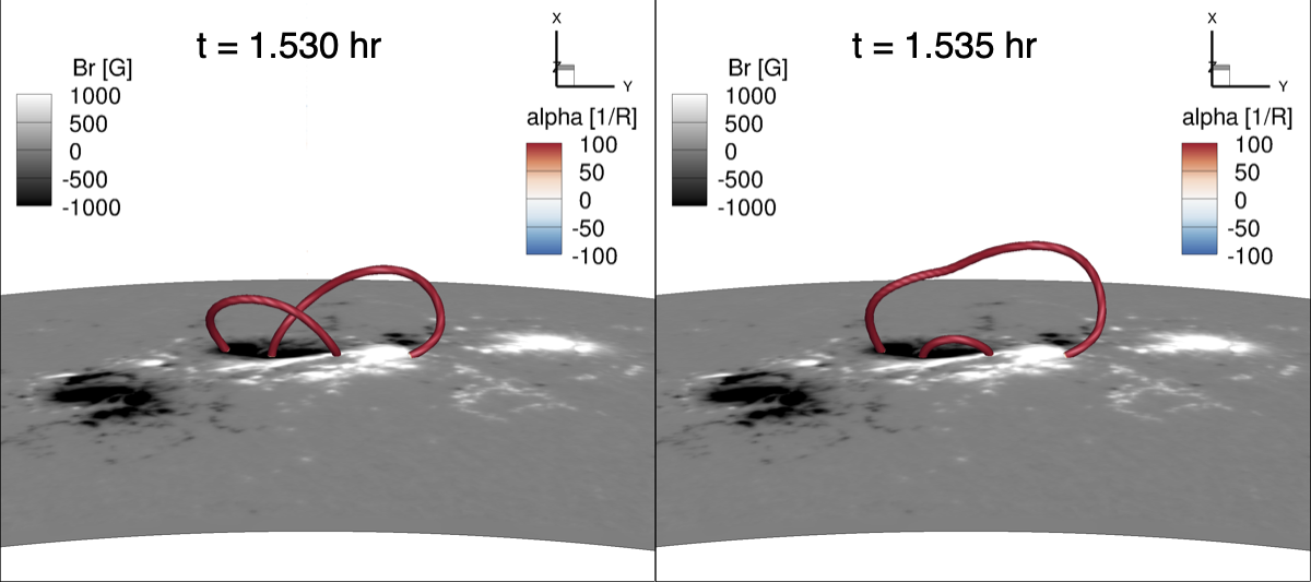
The onset of the tether-cutting reconnection is facilitated by the numerical resistivity, triggered by the thinning of the current sheet in the strongly sheared arcade field above the PIL. Figure 10 shows a 3D view of example field lines before and after undergoing tether-cuttig reconnections. We see that a pair of highly sheared arcade field lines above the central PIL in the earlier time instance (left panel) have reconnected and transformed into a longer dipped field line that erupts upward and a lower short loop that shrinks back down in the later time instance (right panel). The formation of a flux rope with dipped field lines can also be seen in panels (d) and (g) in Figure 8. As the positive-twisted inner field erupts, it encounters and reconnects with the negative-twisted field above (see top row of Fig. 8). Eventually, the erupting field develops a complex structure that consists of an outer flux rope containing mainly negative twist (left-handed twist) and an inner flux rope containing mainly positive twist (right-handed twist) (see panels (m) and (n) in Fig 8), with the outer flux rope accelerating to a speed of about km/s as it approaches the top of the domain (panels (l) and (o) in Fig. 8). It can also be seen in panels (l) and (o) in Fig. 8 (and the associated movie) that the rise velocity of the inner flux rope appears to decelerate towards the end. This is due to its collision and reconnection with the overlying negative twisted flux, which forms the outer flux rope that continues to accelerate and exits the domain while the inner flux rope slows down as it loses twist via reconnection with part of the outer magnetic flux. The top boundary is an open boundary allowing plasma to flow through. However, the side boundaries are closed wall boundaries where both the magnetic and velocity fields become parallel to the walls. Thus the lateral expansion and deflection of the erupting flux ropes are artificially constrained by the side boundaries (see result in the next section).
3.4 The observational signatures of the erupting field
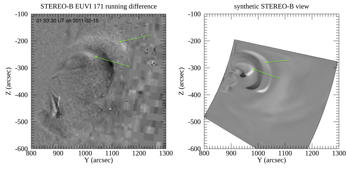
To study the observational signatures of the simulated erupting field, we have computed the synthetic EUV images in the AIA 171 Å channel but viewed from the STEREO-B perspective. The right panel of Figure 11 shows the running difference of two synthetic images at times hour and hour during the eruption. It shows an outgoing double shell structure produced by the two outgoing flux ropes. A running difference image from the observed STEREO-B EUVI 171 passband images during the eruption (left panel of Fig. 11) shows a similar outgoing double-shell structure, although the observed out-going structure expands side-way significantly more than the simulated one because of the constraining side wall boundary of the simulation domain. Simulation with a widened domain is needed for a quantitative comparison of the kinematics of the erupting structure.
CME-associated coronal dimmings are thought to correspond to footpoints of the expanding CME magnetic structures and caused by a density decrease in these structures due to their rapid expansion (e.g. Thompson et al., 1998; Dissauer et al., 2018). Here we use our data-driven simulation to identify the footpoints of the erupting field lines and compare them with the observed EUV dimmings of the CME event. The bottom panels in Figure 12 show the lengths of the field lines traced from each locations at the base of the corona at the onset of the eruption (panel (d)), and at a time when the outer erupting flux rope is exiting the domain (panel (e)), and the difference between the two times (panel (f)) which shows the change of the field line lengths due to the eruption.
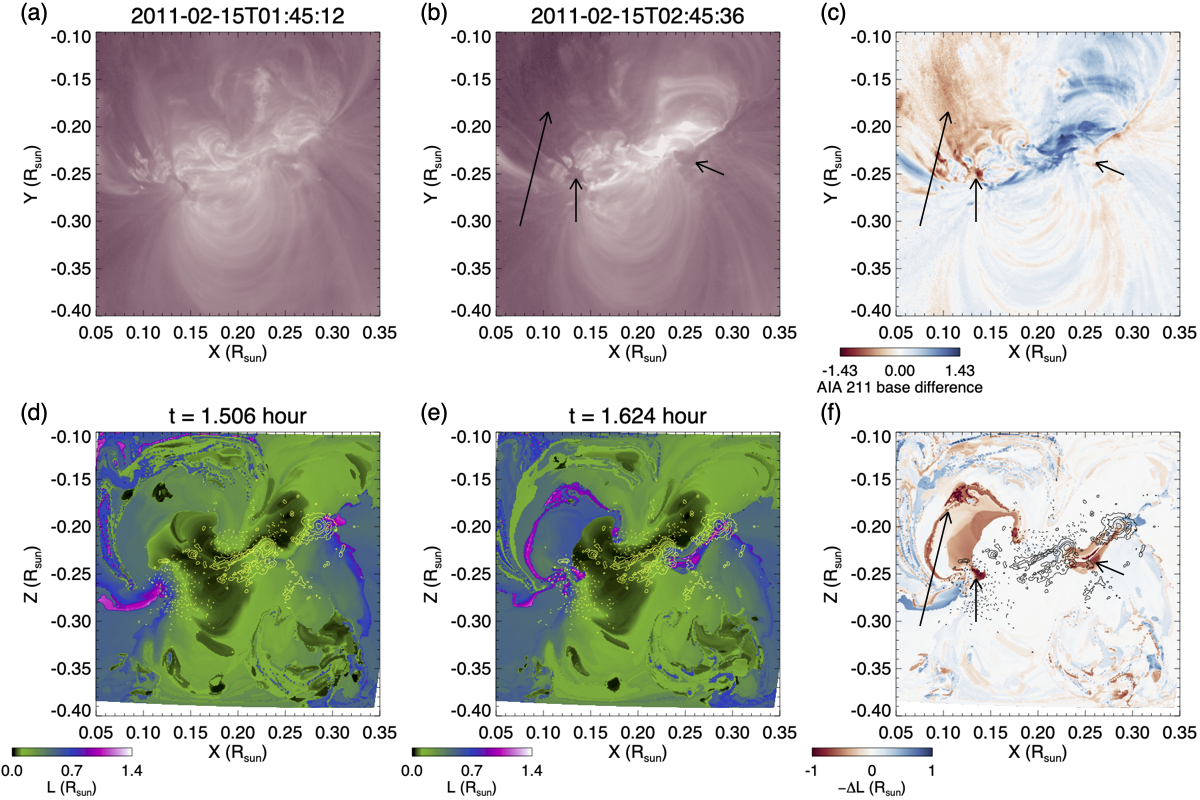
The regions of large field line length increases (as represented by the red patches in panel (f)) correspond to the foot points of the stretched-out erupting field lines. We find that these regions of the erupting field line foot points correspond well with both the two core dimming regions (indicated by the two short arrows) as well as the the more diffuse secondary dimming region (indicated by the long arrow) seen in the AIA 211 Å channel observations (panels (b) and (c)). This agreement adds validation to the modeled erupting field.
Observations have also shown that there is a rapid and irreversible change of the photospheric magnetic field associated with a solar flare (e.g Wang et al., 1994; Sun et al., 2012; Liu et al., 2012) as a result of the “implosion” of the coronal magnetic field just above the flare PIL due to the release of the magnetic energy (Hudson, 2000; Fisher et al., 2012). In Figure 13 we show the change of the horizontal magnetic field strength at the lower boundary 12 min after the onset of the eruption in the simulation compared to the observed change of the horizontal magnetic field strength in the photosphere vector magnetogram 12 min after the onset of the observed X-class flare.
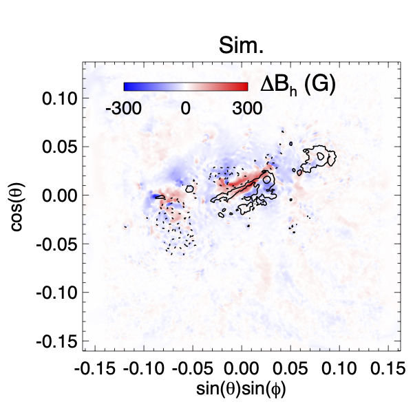
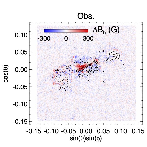
We find that the change of in the simulation shows a similar pattern as the observed change in the central flaring region, where there is a significant enhancement of over the central PIL due to the implosion of the post reconnection loops, while there is a systematic decrease of in the periphery of the flare region away from the central PIL, where the field becomes more vertical as it erupts. This agreement is further evidence that our simulated eruption qualitatively reproduces the magnetic field reconfiguration during the flare.
4 Summary and Discussions
We have performed a boundary data-driven MHD simulation of the eruptive flare and CME that occurred on 2011-02-15 from AR 11158. The simulation is driven at the lower boundary with an electric field derived from the observed evolution of the normal magnetic field and the vertical electric current density measured from the HMI vector magnetograms as described in §2.2. In the simulation, the twisting electric field based on the observed vertical electric current energizes the initial potential field to build up a pre-eruption coronal magnetic field that is close to the NLFFF extrapolation and it subsequently develops multiple eruptions. The sheared/twisted field lines of the pre-eruption magnetic field show morphologies in qualitative agreement with the brightening loops observed in the SDO/AIA hot passband images. From the simulation we find that the eruption is initiated by the tether-cutting reconnection of the highly sheared sigmoid field above the central PIL. After the onset a postive-twisted flux rope with dipped field lines forms during the eruption, which also pushes out and reconnects with an outer negative-twisted field. This interaction results in a complex erupting structure containing two distinct flux ropes, and produces an outgoing double-shell feature similar to that seen in the STEREO-B/EUVI 171 passpand observation of the CME. Furthermore, we find that the foot points of the erupting field lines spatially agree with the major EUV dimming regions of the eruptive flare observed by the SDO/AIA. The change of the horizontal magnetic field at the lower boundary during the simulated eruption also shows a pattern similar to that of the observed change of the photosphere horizontal magnetic field produced by the observed X-class flare. These agreements suggest the validity of the modeled magnetic field evolution for the initiation of this observed CME event.
The twisting electric field used here is a way to establish the non-potential pre-eruption magnetic field in an accelerated time-scale, capturing the cumulative effects of the long-term build up (by e.g. shearing at the PIL and sunspot rotation) as measured by the observed vertical electric current density. It assumes an ad hoc constant transport speed that is not well constrained by observations, and whose value used in the current simulation is crudely selected by trial and error with multiple simulations to best match the observed eruptive behavior for the first eruption. The choice of the value for is strongly influenced by the numerical resistivity in the code in order to build up the pre-eruption electric current against the numerical dissipation, and the use of a constant value of continuously results in the subsequent repeated eruptions which are not in agreement with the observation. Future improvements of the formulation of the twisting electric field to temporally and spatially vary the transport speed based on additional observational constrains are needed to improve the agreement of the modeled eruptive behavior with the observations. One improvement for example is to vary the transport speed based on the difference between the simulated and the observed vertical electric current at the lower boundary.
References
- Afanasyev et al. (2023) Afanasyev, A. N., Fan, Y., Kazachenko, M. D., & Cheung, M. C. M. 2023, ApJ, 952, 136, doi: 10.3847/1538-4357/acd7e9
- Cheung & DeRosa (2012) Cheung, M. C. M., & DeRosa, M. L. 2012, ApJ, 757, 147, doi: 10.1088/0004-637X/757/2/147
- Dahlin et al. (2022) Dahlin, J. T., DeVore, C. R., & Antiochos, S. K. 2022, ApJ, 941, 79, doi: 10.3847/1538-4357/ac9e5a
- Dissauer et al. (2018) Dissauer, K., Veronig, A. M., Temmer, M., Podladchikova, T., & Vanninathan, K. 2018, ApJ, 855, 137, doi: 10.3847/1538-4357/aaadb5
- Fan (2017) Fan, Y. 2017, ApJ, 844, 26, doi: 10.3847/1538-4357/aa7a56
- Fan (2022) —. 2022, ApJ, 941, 61, doi: 10.3847/1538-4357/aca0ec
- Fisher et al. (2012) Fisher, G. H., Bercik, D. J., Welsch, B. T., & Hudson, H. S. 2012, Sol. Phys., 277, 59, doi: 10.1007/s11207-011-9907-2
- Fisher et al. (2020) Fisher, G. H., Kazachenko, M. D., Welsch, B. T., et al. 2020, ApJS, 248, 2, doi: 10.3847/1538-4365/ab8303
- Forbes et al. (2006) Forbes, T. G., Linker, J. A., Chen, J., et al. 2006, Space Sci. Rev., 123, 251, doi: 10.1007/s11214-006-9019-8
- Green et al. (2018) Green, L. M., Török, T., Vršnak, B., Manchester, W., & Veronig, A. 2018, Space Sci. Rev., 214, 46, doi: 10.1007/s11214-017-0462-5
- Gudiksen & Nordlund (2005) Gudiksen, B. V., & Nordlund, Å. 2005, ApJ, 618, 1020, doi: 10.1086/426063
- Hayashi et al. (2018) Hayashi, K., Feng, X., Xiong, M., & Jiang, C. 2018, ApJ, 855, 11, doi: 10.3847/1538-4357/aaacd8
- Hoeksema et al. (2020) Hoeksema, J. T., Abbett, W. P., Bercik, D. J., et al. 2020, ApJS, 250, 28, doi: 10.3847/1538-4365/abb3fb
- Hudson (2000) Hudson, H. S. 2000, ApJ, 531, L75, doi: 10.1086/312516
- Inoue et al. (2014) Inoue, S., Hayashi, K., Magara, T., Choe, G. S., & Park, Y. D. 2014, ApJ, 788, 182, doi: 10.1088/0004-637X/788/2/182
- Inoue et al. (2015) —. 2015, ApJ, 803, 73, doi: 10.1088/0004-637X/803/2/73
- Jiang et al. (2022) Jiang, C., Feng, X., Guo, Y., & Hu, Q. 2022, The Innovation, 3, 100236, doi: 10.1016/j.xinn.2022.100236
- Kazachenko et al. (2014) Kazachenko, M. D., Fisher, G. H., & Welsch, B. T. 2014, ApJ, 795, 17, doi: 10.1088/0004-637X/795/1/17
- Kliem & Török (2006) Kliem, B., & Török, T. 2006, Physical Review Letters, 96, 255002, doi: 10.1103/PhysRevLett.96.255002
- Linton et al. (2023) Linton, M. G., Antiochos, S. K., Barnes, G., et al. 2023, Adv. Space Research, published online, doi: 10.1016/j.asr.2023.06.045
- Liu et al. (2012) Liu, C., Deng, N., Liu, R., et al. 2012, ApJ, 745, L4, doi: 10.1088/2041-8205/745/1/L4
- Mackay et al. (2014) Mackay, D. H., DeVore, C. R., & Antiochos, S. K. 2014, ApJ, 784, 164, doi: 10.1088/0004-637X/784/2/164
- Patsourakos et al. (2020) Patsourakos, S., Vourlidas, A., Török, T., et al. 2020, Space Sci. Rev., 216, 131, doi: 10.1007/s11214-020-00757-9
- Sun et al. (2012) Sun, X., Hoeksema, J. T., Liu, Y., et al. 2012, ApJ, 748, 77, doi: 10.1088/0004-637X/748/2/77
- Temmer (2021) Temmer, M. 2021, Living Reviews in Solar Physics, 18, 4, doi: 10.1007/s41116-021-00030-3
- Thompson et al. (1998) Thompson, B. J., Plunkett, S. P., Gurman, J. B., et al. 1998, Geophys. Res. Lett., 25, 2465, doi: 10.1029/98GL50429
- Wang et al. (1994) Wang, H., Ewell, M. W., J., Zirin, H., & Ai, G. 1994, ApJ, 424, 436, doi: 10.1086/173901
- Warnecke & Peter (2019) Warnecke, J., & Peter, H. 2019, A&A, 624, L12, doi: 10.1051/0004-6361/201935385
- Wheatland et al. (2000) Wheatland, M. S., Sturrock, P. A., & Roumeliotis, G. 2000, ApJ, 540, 1150, doi: 10.1086/309355