A decoupled structure preserving scheme for the Poisson-Nernst-Planck Navier-Stokes equations and its error analysis

Ziyao Yu^†, Jie Shen^⋆, Changyou Wang^†, Qing Cheng^‡

Abstract.

We consider in this paper numerical approximations for the Poisson-Nernst-Planck-Navier-Stokes (PNP-NS) system. We propose a decoupled semi-discrete and fully discrete scheme that enjoys the nice properties of positivity preserving, mass conserving, and unconditionally energy stability. Then, we establish the well-posedness and regularity for the initial and (periodic) boundary value problem of the PNP-NS system under suitable assumptions on the initial data, and carry out a rigorous convergence analysis for the fully discretized scheme. We also present some numerical results to validate the positivity preserving property and the accuracy for our decoupled numerical scheme.

Keywords. Error analysis; PNP-NS system; Unique Solvability; Structure-preserving; Positivity-preserving.

Cheng is supported in parts by NSFC 12301522 and the Fundamental Research Funds for the Central Universities, Shen is supported in parts by NSFC 11971407, and Wang is supported in parts by NSF 2101224. The main contents of this paper are part of Z. Yu’s Ph.D thesis at Purdue University.

^† Department of Mathematics, West Lafayette, IN 47907, USA (yu583@purdue.edu, wang2482@purdue.edu).
^‡Key Laboratory of Intelligent Computing and Application (Tongji University), Ministry of Education, and Department of Mathematics, Tongji University, Shanghai 200092, P. R. China (qingcheng@tongji.edu.cn).
^⋆ Eastern Institute of Technology, Ningbo, Zhejiang 315200, P. R. China (jshen@eitech.edu.cn).

1. Introduction

In this paper, we consider a time-dependent system that describes the electrodiffusion of ions in an isothermal, incompressible, and viscous Newtonian fluid. Such a system is called the Poisson-Nernst-Planck-Navier-Stokes (PNP-NS) system gong2021partial ; liu2021positivity ; schmuck2011modeling , which is widely applied in fields such as microfluids which has numerous applications in lab-on-a-chip system; biology including vesicle motion, membrane fluctuations, electroporation; and electrochemistry such as porous electrode charging, desalination dynamics, dendritic growth bazant2010induced . An introduction to some basic physical and mathematical descriptions can be found in rubinstein1990electro .

We consider a solution of a monovalent symmetric strong salt. The Poisson-Nernst-Planck equations and incompressible Navier-Stokes Equations describe the system as

	$\displaystyle p_{t}+({\bf u}\cdot\nabla)p=D\nabla\cdot(\nabla p+\frac{e}{k_{B}T}p\nabla\Psi),$
	$\displaystyle n_{t}+({\bf u}\cdot\nabla)n=D\nabla\cdot(\nabla n-\frac{e}{k_{B}T}n\nabla\Psi),$
	$\displaystyle-\epsilon\Delta\Psi=\rho_{e},$
	$\displaystyle{\bf u}_{t}+({\bf u}\cdot\nabla){\bf u}-\nu_{vis}\Delta{\bf u}+\nabla P=-\nabla\Psi\rho_{e},$
	$\displaystyle\nabla\cdot{\bf u}=0,$

where ${\bf u}$ and $P$ denote the velocity field of the fluid and the pressure function, respectively. The variables $p$ and $n$ represent the concentration functions of positive and negative ions in the fluid, respectively, and $\Psi$ is the electric potential. Here $\rho_{e}=e(p-n)$ represents the free charge density for a monovalent symmetric salt (here ionic valence $z=\pm 1$ ), and $e$ is elementary charge. $k_{B}$ is Boltzemann’s constant, $T$ is temperature and $D$ is the diffusion coefficient of ions. Moreover, $\epsilon$ , $\nu_{vis}$ are the dielectric permittivity and viscosity of the fluid. Normalizing the electric potential by introducing $\psi$ : $\psi=\frac{e}{k_{B}T}\Psi.$ The PNP-NS system is therefore given by

(1.1)		$\displaystyle p_{t}+({\bf u}\cdot\nabla)p=D\nabla\cdot(\nabla p+p\nabla\psi),$
(1.2)		$\displaystyle n_{t}+({\bf u}\cdot\nabla)n=D\nabla\cdot(\nabla n-n\nabla\psi),$
(1.3)		$\displaystyle-\varepsilon\Delta\psi=p-n,$
(1.4)		$\displaystyle{\bf u}_{t}+({\bf u}\cdot\nabla){\bf u}-\nu_{vis}\Delta{\bf u}+\nabla P=-\kappa\nabla\psi(p-n),$
(1.5)		$\displaystyle\nabla\cdot{\bf u}=0,$

with $\varepsilon=\frac{\epsilon k_{B}T}{e^{2}}$ , and $\kappa=k_{B}T$ . It is worth to note that $\varepsilon=2c_{bulk}\lambda_{D}^{2}$ , where $\lambda_{D}$ is the Debye screening length bazant2010induced defined by $\lambda_{D}=\sqrt{\frac{\epsilon k_{B}T}{2c_{\text{bulk}}e^{2}}}$ and $c_{\text{bulk}}$ is a reference bulk concentration of ions. The system (1.1)-(1.5) is subjected to a set of initial and boundary conditions, which will be specified later.

There has been considerable interest in the mathematical analysis of the PNP-NS system. For example, Schmuck schmuck2009analysis established the global existence of weak solutions in three dimensions under the blocking boundary condition for $(p,n)$ and the zero Neumann boundary condition for $\psi$ ; Gong-Wang-Zhang gong2021partial established the existence and partial regularity of suitable weak solutions in three dimensions under the zero Neumann boundary condition for $p$ , $n$ , and $\psi$ ; Constantin-Ignatova constantin2019nernst proved the global existence and stability result in two dimensions, with the blocking and selective boundary conditions for $(p,n)$ and the Dirichlet boundary condition for $\psi$ . We emphasize that the solutions of the PNP-NS system are positive ( $n,p>0$ ), mass-conserving, and energy-dissipative.

In recent years, a large effort has been devoted to constructing positivity-preserving schemes for various problems in different areas MR4186541 ; MR4107225 ; MR3880256 ; MR4253790 ; liu2018positivity ; van2019positivity ; shen2016maximum ; zhornitskaya1999positivity ; chen2019positivity . There are also quite a few numerical investigations on the PNP-NS system (1.1)-(1.5). It was shown in flavell2014conservative that it is important for numerical schemes to maintain mass conservation. Prohl-Schmuck proposed in prohl2010convergent a coupled fully implicit first-order scheme with a finite-element method in space for the PNP-NS system and studied its convergence. Additionally, a first-order time-stepping method was proposed in liu2017efficient with spectral method discretization in space. Several structure-preserving numerical methods have been proposed for the PNP equations, for example, cheng2022new2 ; cheng2022new ; flavell2014conservative ; hu2020fully ; huang2021bound ; liu2021positivity ; prohl2009convergent ; shen2021unconditionally ; liu2021efficient ; ding2019positivity . There are also some recent studies reformulate the PNP system into Maxwell-Ampere Nernst-Planck(MANP) system qiao2023structure . However, there appears to be no scheme available in the literature for the PNP-NS system (1.1)-(1.5) that enjoys the properties of unique solvability, mass- and positivity-preserving, and energy stability.

In this paper, we propose a decoupled, mass- and positivity-preserving, and unconditionally energy-stable scheme for the PNP-NS system and carry out a rigorous error analysis. The main contributions of this paper include:

•
We propose a totally decoupled, mass- and positivity-preserving, and unconditionally energy-stable scheme for the PNP-NS system by combining the following techniques:
- –
  
  Rewriting the PNP system as a Wasserstein gradient flow and using the technique introduced in shen2021unconditionally to preserve positivity and energy stability for the PNP system;
- –
  
  Using a projection-type method guermond2006overview ; guermond1998approximation ; guermond1998stability to decouple the velocity and pressure;
- –
  
  Introducing an extra $\mathcal{O}(\Delta t)$ term as in shen2015decoupled , which allows us to treat the convective term in the PNP equations explicitly while maintaining stability.
•

We derive the existence and regularity results of the PNP-NS system (1.1)-(1.5) with periodic boundary conditions under suitable assumptions on the initial data.
•

To carry out an error analysis, it is necessary to have $L^{\infty}$ bounds for $n$ and $p$ , which are not available through energy stability. We use an approach similar to liu2021positivity to derive these bounds by introducing a high-order asymptotic expansion for both the PNP equations and the Navier-Stokes equations.

This paper is organized as follows: In Section 2, we construct a semi-discrete (in time) scheme, followed by a fully discrete scheme with a generic spatial discretization, and prove that it preserves mass and positivity, and is unconditionally energy stable. In Section 3, we establish the well-posedness and regularity of the PNP-NS system under periodic boundary conditions. An error analysis of the fully discretized scheme is carried out in Section 4. Some numerical results are provided in Section 5.

2. A Decoupled Numerical Scheme and Its Properties

Let $\Omega$ be a bounded domain in $\mathbb{R}^{2}$ . We consider the time discretization of the PNP-NS system (1.1)-(1.5) subjected to boundary condition either

•

$\mathcal{B}^{block}$ : the non-slip boundary condition for ${\bf u}$ , the homogeneous Neumann boundary condition for $(\phi,\ln{p}+\psi,\ln{n}-\psi)$ , i.e., all the fluxes vanish on the boundary of $\Omega$ :

(2.1)

{\bf u}|_{\partial\Omega}=0,\;\;\nabla\phi\cdot\vec{\nu}\big{|}_{\partial\Omega}=(\nabla p+p\nabla\psi)\cdot\vec{\nu}\big{|}_{\partial\Omega}=(\nabla n-n\nabla\psi)\cdot\vec{\nu}\big{|}_{\partial\Omega}=0,

•

$\mathcal{B}^{periodic}$ : the periodic boundary conditions for all variables,

along with the initial condition:

(2.2)

\displaystyle({\bf u},p,n)(x,y,0)=({\bf u}^{\text{in}},p^{\text{in}},n^{\text{in}})(x,y),\quad\text{for}\ (x,y)\in\Omega.

For either (2.1) or the periodic boundary conditions, one observes that the mass of ions is conserved, i.e.,

\int_{\Omega}p(x,t)\,dx=\int_{\Omega}p(x,0)\,dx,\quad\int_{\Omega}n(x,t)\,dx=\int_{\Omega}n(x,0)\,dx,\quad\forall t\in[0,T].

Another essential property of the PNP-NS system (1.1)-(1.5) is the following energy dissipation law:

(2.3)

\frac{d}{dt}E(p,n,{\bf u})=-\int_{\Omega}\left({\color[rgb]{0,0,1}\definecolor[named]{pgfstrokecolor}{rgb}{0,0,1}\nu_{vis}}\rvert\nabla{\bf u}\rvert^{2}+{\color[rgb]{0,0,1}\definecolor[named]{pgfstrokecolor}{rgb}{0,0,1}\kappa D}p\rvert\nabla\mu\rvert^{2}+{\color[rgb]{0,0,1}\definecolor[named]{pgfstrokecolor}{rgb}{0,0,1}\kappa D}n\rvert\nabla\nu\rvert^{2}\right)dx,

where $\mu=\ln{p}+\psi$ and $\nu=\ln{n}-\psi$ are chemical potentials of the PNP-NS system, and $E$ is the total energy given by

E(p,n,{\bf u})=\int_{\Omega}{\color[rgb]{0,0,1}\definecolor[named]{pgfstrokecolor}{rgb}{0,0,1}\kappa}\left(p(\ln{p}-1)+n(\ln{n}-1)+\frac{\varepsilon}{2}\rvert\nabla\psi\rvert^{2}\right)+\frac{1}{2}\rvert{\bf u}\rvert^{2}dx.

2.1. Time Discretization

We first consider the time discretization. For simplicity, we set various constants $D=\varepsilon=\kappa=\nu_{vis}=1$ for the rest analysis. In order to construct an efficient time discretization scheme, we first rewrite the right-hand side of equation (1.4) as

-\nabla\psi(p-n)=-(p\nabla\mu+n\nabla\nu)+\nabla(p+n),

and introduce a modified pressure $\phi=P-p-n$ . Then, the PNP-NS system (1.1)-(1.5) can be reformulated as

(2.4)		$\displaystyle p_{t}+({\bf u}\cdot\nabla)p=\nabla\cdot(p\nabla\mu),$
(2.5)		$\displaystyle n_{t}+({\bf u}\cdot\nabla)n=\nabla\cdot(n\nabla\nu),$
(2.6)		$\displaystyle-\Delta\psi=p-n,$
(2.7)		$\displaystyle{\bf u}_{t}+({\bf u}\cdot\nabla){\bf u}-\Delta{\bf u}+\nabla\phi=-(p\nabla\mu+n\nabla\nu),$
(2.8)		$\displaystyle\nabla\cdot{\bf u}=0.$

Depending on boundary condition choice $\mathcal{B}$ , we define the function space $X(\mathcal{B}),U(\mathcal{B}),W(\mathcal{B})$ :

•

$X(\mathcal{B}^{block})=X(\mathcal{B}^{periodic})=H^{1}(\Omega)$ ,
•

$U(\mathcal{B}^{block})=U(\mathcal{B}^{periodic})=\{q\in L^{2}(\Omega):\int_{\Omega}q\,dx=0\}$ ,
•

$W(\mathcal{B})=\big{\{}\begin{array}[]{l}H^{1}_{0}(\Omega),\text{ if }\mathcal{B}=\mathcal{B}^{block},\\ H^{1}(\Omega),\text{ if }\mathcal{B}=\mathcal{B}^{periodic}.\end{array}$

Following some of the ideas in shen2021unconditionally ; liu2021positivity ; shen2015decoupled , we construct a first-order time discretization scheme as follows: under boundary condition $\mathcal{B}$ being either $\mathcal{B}^{block}$ or $\mathcal{B}^{periodic}$ , for any given $(p^{m},n^{m},{\bf u}^{m},\phi^{m})$ with $\int_{\Omega}(p^{m}-n^{m})\,dx=0$ , $(p^{m},n^{m})>0$ and $\nabla\cdot{\bf u}^{m}=0$ in $\Omega$ , we compute $(p^{m+1},n^{m+1},{\bf u}^{m+1},\phi^{m+1})$ in three steps:

•

Step 1: Solve ${\color[rgb]{0,0,1}\definecolor[named]{pgfstrokecolor}{rgb}{0,0,1}(p^{m+1},n^{m+1})\in X(\mathcal{B})\times X(\mathcal{B})}$ from

(2.9)		$\displaystyle\frac{p^{m+1}-p^{m}}{\Delta t}+\nabla\cdot(p^{m}{\bf u}^{m})=\nabla\cdot(p^{m}(1+2\Delta tp^{m})\nabla\mu^{m+1}),$
(2.10)		$\displaystyle\frac{n^{m+1}-n^{m}}{\Delta t}+\nabla\cdot(n^{m}{\bf u}^{m})=\nabla\cdot(n^{m}(1+2\Delta tn^{m})\nabla\nu^{m+1}),$
(2.11)		$\displaystyle-\Delta\psi^{m+1}=p^{m+1}-n^{m+1}.$

where

\mu^{m+1}=\ln{p^{m+1}}+\psi^{m+1}\quad{\text{and}}\quad\nu^{m+1}=\ln{n^{m+1}}-\psi^{m+1}.

•

Step 2: Solve ${\color[rgb]{0,0,1}\definecolor[named]{pgfstrokecolor}{rgb}{0,0,1}\tilde{{\bf u}}^{m+1}\in W(\mathcal{B})^{2}}$ from

(2.12)

\frac{\tilde{{\bf u}}^{m+1}-{\bf u}^{m}}{\Delta t}+({\bf u}^{m}\cdot\nabla)\tilde{{\bf u}}^{m+1}-\Delta\tilde{{\bf u}}^{m+1}+\nabla\phi^{m}=-\left(p^{m}\nabla\mu^{m+1}+n^{m}\nabla\nu^{m+1}\right),

•

Step 3: Solve ${\color[rgb]{0,0,1}\definecolor[named]{pgfstrokecolor}{rgb}{0,0,1}({\bf u}^{m+1},\phi^{m+1})\in W(\mathcal{B})^{2}\times U(\mathcal{B})}$ from

(2.13)		$\displaystyle\frac{{\bf u}^{m+1}-\tilde{{\bf u}}^{m+1}}{\Delta t}+\nabla(\phi^{m+1}-\phi^{m})=0,$
(2.14)		$\displaystyle\nabla\cdot{\bf u}^{m+1}=0.$

The first step involves solving a coupled nonlinear system for $(p^{m+1},n^{m+1},\psi^{m+1})$ which can be formulated as a minimization problem for a convex functional, see shen2021unconditionally and also Theorem 2.2. The second step solves a Poisson-type equation for $\tilde{{\bf u}}^{m+1}$ . And the third step is equivalent to solving

(2.15)

\displaystyle\Delta(\phi^{m+1}-\phi^{m})=\frac{1}{\Delta t}\nabla\cdot\tilde{{\bf u}}^{m+1},

along with either $(\phi^{m+1}-\phi^{m})\cdot\vec{\nu}\big{|}_{\partial\Omega}=0$ or the periodic boundary condition, and

(2.16)

\displaystyle{\color[rgb]{0,0,1}\definecolor[named]{pgfstrokecolor}{rgb}{0,0,1}{\bf u}^{m+1}}=\tilde{{\bf u}}^{m+1}-\Delta t\nabla(\phi^{m+1}-\phi^{m}).

Thus, the scheme (2.9)-(2.14) can be efficiently implemented.

Remark 1.

In (2.9) (2.10), we discretized the mobility term as $p^{m}(1+2\Delta tp^{m})$ , $n^{m}(1+2\Delta tn^{m})$ , moving the $\mathcal{O}(\Delta t)$ terms to the left, therefore the first step can be rewritten as:

	$\displaystyle\frac{p^{m+1}-p^{m}}{\Delta t}+\nabla\cdot(p^{m}{\bf u}^{m}_{*,p})=\nabla\cdot(p^{m}\nabla\mu^{m+1}),$
	$\displaystyle\frac{n^{m+1}-n^{m}}{\Delta t}+\nabla\cdot(n^{m}{\bf u}^{m}_{*,n})=\nabla\cdot(n^{m}\nabla\nu^{m+1}),$

where

	$\displaystyle{\bf u}^{m}_{*,p}={\bf u}^{m}-2\Delta tp^{m}\nabla\mu^{m+1},$
	$\displaystyle{\bf u}^{m}_{*,n}={\bf u}^{m}-2\Delta tn^{m}\nabla\nu^{m+1}.$

This is similar to the decoupling technique introduced by shen2015decoupled , where specific additional $\mathcal{O}(\Delta t)$ terms are introduced such that the decoupled discrete numerical scheme is unconditionally energy stable, see Theorem 2.2 below.

2.2. Fully Discretized Scheme

In this subsection, we shall consider a generic spatial discretization for (2.9)-(2.14). Let $\Sigma_{N}$ be a set of mesh points or collocation points in $\bar{\Omega}$ . Note that $\Sigma_{N}$ should not include the points on the part of the boundary where a Dirichlet (or essential) boundary condition is prescribed, while it should include the points on the part of the boundary where a Neumann or mixed (or non-essential) boundary condition is prescribed.

We consider a Galerkin-type discretization with finite elements, spectral methods, or finite differences with summation-by-parts in a subspace $X_{N}\subset X$ , and define a discrete inner product, i.e., numerical integration, on $\Sigma_{N}=\{\boldsymbol{z}\}$ in $\bar{\Omega}$ :

(2.17)

\langle u_{N},v_{N}\rangle_{N,\omega}=\sum_{\boldsymbol{z}\in\Sigma_{N}}\omega_{\boldsymbol{z}}u_{N}(\boldsymbol{z})v_{N}(\boldsymbol{z}),

where we require that the weights $\omega_{\boldsymbol{z}}>0$ . We also denote the induced norm by $\|u_{N}\|=\langle u_{N},u_{N}\rangle_{N,\omega}^{\frac{1}{2}}$ . For finite element methods, the sum should be understood as $\sum_{K\subset\mathcal{T}}\sum_{\boldsymbol{z}\in Z(K)}$ , where $\mathcal{T}$ is a given triangulation. We assume that there is a unique function $\psi_{\boldsymbol{z}}(\boldsymbol{x})$ satisfying $\psi_{\boldsymbol{z}}(\boldsymbol{z}^{\prime})=\delta_{\boldsymbol{z}\boldsymbol{z}^{\prime}}$ for $\boldsymbol{z},\boldsymbol{z}^{\prime}\in\Sigma_{N}$ . Under boundary condition $\mathcal{B}$ , let $X_{N}$ , ${W}_{N}$ , and ${U}_{N}$ be suitable discretization subspaces of $X(\mathcal{B})$ , $W(\mathcal{B})$ , and $U(\mathcal{B})$ , respectively.

To fix the idea and without loss of generality, throughout the rest of the paper, reader can think we are discussing under spectral method discretization framework, and $X_{N},W_{N},U_{N}$ are subspaces of $P_{N}$ , where

P_{N}:=\big{\{}\begin{array}[]{l}span\{e^{\mathrm{i}jx}e^{\mathrm{i}ky}:-\frac{N}{2}\leq k\leq\frac{N}{2}-1\},\text{ if }\mathcal{B}=\mathcal{B}^{periodic},\\ span\{1,x,y,xy,...,x^{N}y^{N}\},\text{ if }\mathcal{B}=\mathcal{B}^{block}.\end{array}

Under spectral method framework, the quadrature error is very small when $N$ is large enough, and avoidable in numerical implementation by choosing quadrature points numbers $N_{Q}$ bigger than basis numbers $N$ . For simplicity, throughout the rest of the paper, we ignore the quadrature error, and do not distinguish the continuous inner product $\langle u_{N},v_{N}\rangle$ and discrete inner product $\langle u_{N},v_{N}\rangle_{N,\omega}$ .

Then, a fully discretized version of (2.9)-(2.14) for the PNP-NS system (2.4)-(2.8) is as follows:

Given $(p_{N}^{m},n_{N}^{m},{\bf u}_{N}^{m},\phi_{N}^{m})\in X_{N}\times X_{N}\times{{W}_{N}^{2}}\times{{U}_{N}}$ , with $p_{N}^{m},n_{N}^{m}>0$ in $\Omega$ , $\displaystyle\langle p_{N}^{m}-n^{m}_{N},1\rangle=0$ , and $\nabla\cdot\mathbf{u}_{N}^{m}=0$ in $\Omega$ , we proceed as follows:

•

Step 1: Solve $(p^{m+1}_{N},n^{m+1}_{N})\in X_{N}\times X_{N}$ from

(2.18)		$\displaystyle\langle\frac{p^{m+1}_{N}-p^{m}_{N}}{\Delta t},v_{N}\rangle-\langle p^{m}_{N}{\bf u}^{m}_{N},\nabla v_{N}\rangle+\langle p^{m}_{N}(1+2\Delta tp^{m}_{N})\nabla\mu^{m+1}_{N},\nabla v_{N}\rangle=0,\;\forall v_{N}\in X_{N},\vskip 5.0pt$
(2.19)		$\displaystyle\langle\frac{n^{m+1}_{N}-n^{m}_{N}}{\Delta t},v_{N}\rangle-\langle n^{m}_{N}{\bf u}^{m}_{N},\nabla v_{N}\rangle+\langle n^{m}_{N}(1+2\Delta tn^{m}_{N})\nabla\nu^{m+1}_{N},\nabla v_{N}\rangle=0,\;\forall v_{N}\in X_{N},\vskip 5.0pt$
(2.20)		$\displaystyle\langle\nabla\psi^{m+1}_{N},\nabla v_{N}\rangle=\langle p^{m+1}_{N}-n^{m+1}_{N},v_{N}\rangle,\;\forall v_{N}\in X_{N},\vskip 5.0pt$

where

(2.21)

\mu^{m+1}_{N}=\ln{p^{m+1}_{N}}+\psi^{m+1}_{N},\quad\nu^{m+1}_{N}=\ln{n^{m+1}_{N}}-\psi^{m+1}_{N}.

•

Step 2: Solve $\tilde{{\bf u}}^{m+1}_{N}\in{{W}_{N}^{2}}$ from

	$\displaystyle\langle\frac{\tilde{{\bf u}}^{m+1}_{N}-{\bf u}^{m}_{N}}{\Delta t},{{w_{N}}}\rangle+\langle({\bf u}^{m}_{N}\cdot\nabla)\tilde{{\bf u}}^{m+1}_{N},{{w_{N}}}\rangle+\langle\nabla\tilde{{\bf u}}^{m+1}_{N},\nabla{{w_{N}}}\rangle+\langle\nabla\phi^{m}_{N},w_{N}\rangle,$
(2.22)		$\displaystyle\qquad+\langle p^{m}_{N}\nabla\mu^{m+1}_{N}+n^{m}_{N}\nabla\nu^{m+1}_{N},{{w_{N}}}\rangle=0,\;\forall w_{N}\in{{W}_{N}^{2}},\vskip 5.0pt$

•

Step 3: Solve $({\bf u}^{m+1}_{N},\phi^{m+1}_{N})\in{{W}_{N}^{2}}\times{{U}_{N}}$ from

(2.23)		$\displaystyle\langle\frac{{\bf u}^{m+1}_{N}-\tilde{{\bf u}}^{m+1}_{N}}{\Delta t},v_{N}\rangle+\langle\nabla(\phi^{m+1}_{N}-\phi^{m}_{N}),v_{N}\rangle=0,\;v_{N}\in X_{N}^{2},$
(2.24)		$\displaystyle{{\langle{\bf u}^{m+1}_{N},\nabla q_{N}\rangle}}=0,\;q_{N}\in{{U}_{N}}.$

We shall show below that the nonlinear system (2.18)-(2.20) in Step 1 can be interpreted as a minimization of a convex functional. In Step 2, we only need to solve a Poisson-type equation for $\tilde{{\bf u}}^{m+1}_{N}$ , and Step 3 is a discrete Darcy system which can be reduced to a discrete Poisson equation for $\phi^{m+1}_{N}-\phi^{m}_{N}$ . Hence, the above scheme can be efficiently solved.

2.3. Properties of the Numerical Scheme

We show below that our decoupled numerical scheme (2.18)-(2.24) enjoys four properties: mass conservation, unique solvability, positivity-preserving, and unconditional energy stability.

Before proceeding to the proof, for any discrete positive function $\mathcal{M}({\bf z})>0$ for all ${\bf z}\in\Sigma_{N}$ , we introduce the operator $\mathcal{L}_{\mathcal{M}}:X_{N}\rightarrow X_{N}$ defined by

(2.25)

\langle\mathcal{L}_{\mathcal{M}}f_{N},v_{N}\rangle=\langle\mathcal{M}\nabla f_{N},\nabla v_{N}\rangle,\quad\forall f_{N},v_{N}\in X_{N}.

The operator $\mathcal{L}_{\mathcal{M}}$ is invertible on the space $\dot{X}_{N}=\big{\{}f\in X_{N}\mid\langle f,1\rangle=0\big{\}}$ , so we can define the inverse operator $\mathcal{L}^{-1}_{\mathcal{M}}:X_{N}\rightarrow\dot{X}_{N}$ and the induced norm

\|f_{N}\|_{\mathcal{L}^{-1}_{\mathcal{M}}}=\sqrt{\langle f_{N},\mathcal{L}_{\mathcal{M}}^{-1}f_{N}\rangle},\quad\forall f_{N}\in X_{N}.

If $\mathcal{M}({\bf z})\equiv 1$ for all ${\bf z}\in\Sigma_{N}$ , then we have

\mathcal{L}_{\mathcal{M}}(f_{N})=-\Delta f_{N}\quad\text{and}\quad\|f_{N}\|_{-1,\Omega}=\sqrt{\langle f_{N},(-\Delta)^{-1}f_{N}\rangle},\quad\forall f_{N}\in X_{N}.

Lemma 2.1.

Suppose $f_{N}\in X_{N}$ and $\mathcal{M}\geq M_{0}$ , then we have the estimate:

\|\mathcal{L}^{-1}_{\mathcal{M}}f_{N}\|_{\infty}\leq\frac{C{\color[rgb]{0,0,1}\definecolor[named]{pgfstrokecolor}{rgb}{0,0,1}N}}{M_{0}}\|f_{N}\|,

where $C$ depends only on $\Omega$ .

Proof.

Denote $u_{N}=\mathcal{L}^{-1}_{\mathcal{M}}f_{N}\in{\color[rgb]{0,0,1}\definecolor[named]{pgfstrokecolor}{rgb}{0,0,1}\dot{X}_{N}}$ . From (2.25) and using the Poincaré-Wirtinger inequality, we have

M_{0}\|\nabla u_{N}\|^{2}\leq\langle\mathcal{M}\nabla u_{N},\nabla u_{N}\rangle=\langle f_{N},u_{N}\rangle\leq\|f_{N}\|\|u_{N}\|\leq C\|f_{N}\|\|\nabla u_{N}\|,

and applying the Nikolskii’s inequality, we have

\|u_{N}\|_{\infty}\leq C(\Omega)N\|u\|_{2}\leq C(\Omega)N\|\nabla u_{N}\|\leq\frac{CN}{M_{0}}\|f_{N}\|,

where $C$ depends only on $\Omega$ . ∎

Theorem 2.2.

Given $(p^{m}_{N},n^{m}_{N},{\bf u}^{m}_{N},\phi^{m}_{N})\in X_{N}\times X_{N}\times{W}_{N}^{2}\times{U}_{N}$ , with $p_{N}^{m}({\bf z}),n_{N}^{m}({\bf z})>0$ for all ${\bf z}\in\Sigma_{N}$ , $\displaystyle\langle p_{N}^{m}-n^{m}_{N},1\rangle=0$ , and $\nabla\cdot\mathbf{u}_{N}^{m}=0$ in $\Omega$ , then the scheme (2.18)-(2.24) enjoys the following properties:

(1)

Mass Conservation:

$\langle p^{m+1}_{N},1\rangle=\langle p^{m}_{N},1\rangle,\quad\langle n^{m+1}_{N},1\rangle=\langle n^{m}_{N},1\rangle.$
(2)

Unique Solvability: The scheme (2.18)-(2.23) has a unique solution

$(p^{m+1}_{N},n^{m+1}_{N},{\bf u}^{m+1}_{N},\phi^{m+1}_{N})\in X_{N}\times X_{N}\times{W}_{N}^{2}\times{U}_{N}.$
(3)

Positivity Preserving: The unique solution $(p^{m+1}_{N},n^{m+1}_{N},{\bf u}^{m+1}_{N},\phi^{m+1}_{N})$ satisfies

$p^{m+1}_{N}({\bf z}),\,n^{m+1}_{N}({\bf z})>0,\quad\forall{\bf z}\in\Sigma_{N}.$

(4)

Unconditional Energy Stability:

\begin{split}&\quad\frac{1}{\Delta t}\bigg{(}\big{(}E(p^{m+1}_{N})+E(n^{m+1}_{N})+\frac{1}{2}\|\nabla\psi^{m+1}_{N}\|^{2}+\frac{1}{2}\|{\bf u}^{m+1}_{N}\|^{2}+\frac{\Delta t^{2}}{2}\|\nabla\phi^{m+1}_{N}\|^{2}\big{)}\\ &\quad-\big{(}E(p^{m}_{N})+E(n^{m}_{N})+\frac{1}{2}\|\nabla\psi^{m}_{N}\|^{2}+\frac{1}{2}\|{\bf u}^{m}_{N}\|^{2}+\frac{\Delta t^{2}}{2}\|\nabla\phi^{m}_{N}\|^{2}\big{)}\bigg{)}\\ &\quad+\|\nabla\tilde{{\bf u}}^{m+1}_{N}\|^{2}+\langle p^{m}_{N}|\nabla\mu^{m+1}_{N}|^{2},1\rangle+\langle n^{m}_{N}|\nabla\nu^{m+1}_{N}|^{2},1\rangle\\ &\quad+\frac{1}{2\Delta t}\|\nabla(\psi^{m+1}_{N}-\psi^{m}_{N})\|^{2}+\frac{1}{2\Delta t}\|{\bf u}^{m+1}_{N}-\tilde{{\bf u}}^{m+1}_{N}\|^{2}\\ &\quad+\frac{1}{2\Delta t}\|\tilde{{\bf u}}^{m+1}_{N}-{\bf u}^{m}_{N}\|^{2}+\frac{\Delta t}{2}\|\nabla(\phi^{m+1}_{N}-\phi^{m}_{N})\|^{2}\\ &\leq-\|\nabla\tilde{{\bf u}}^{m+1}_{N}\|^{2}-\langle p^{m}_{N}|\nabla\mu^{m+1}_{N}|^{2},1\rangle-\langle n^{m}_{N}|\nabla\nu^{m+1}_{N}|^{2},1\rangle.\end{split}

where the energy is defined by

E(v_{N})=\langle v_{N}(\ln{v_{N}}-1),1\rangle,

for any function $v_{N}\in X_{N}$ .

Proof.

(1)

Mass Conservation: This follows directly by choosing the test function $v_{N}=1$ in the equations (2.18) and (2.19).

(2)

Unique Solvability and Positivity Preserving: The numerical solution $\{p^{m+1}_{N},n^{m+1}_{N}\}$ of (2.18)-(2.20) is obtained through the minimization of the discrete energy functional:

\begin{split}J(p^{*}_{N},n^{*}_{N})&=\frac{1}{2\Delta t}\Big{(}\|p^{*}_{N}-p^{m}_{N}\|_{\mathcal{L}^{-1}_{p^{m}_{N}(1+2\Delta tp^{m}_{N})}}^{2}+\|n^{*}_{N}-n^{m}_{N}\|_{\mathcal{L}^{-1}_{n^{m}_{N}(1+2\Delta tn^{m}_{N})}}^{2}\Big{)}\\ &\quad+\langle\nabla\cdot(p^{m}_{N}\mathbf{u}_{N}^{m})p^{*}_{N},1\rangle+\langle\nabla\cdot(n^{m}_{N}\mathbf{u}_{N}^{m})n^{*}_{N},1\rangle\\ &\quad+\langle p^{*}_{N}(\ln{p^{*}_{N}}-1),1\rangle+\langle n^{*}_{N}(\ln{n^{*}_{N}}-1),1\rangle+\frac{1}{2}\|p^{*}_{N}-n^{*}_{N}\|_{-1,\Omega}^{2},\end{split}

over the admissible space

\hat{Y}_{N}=\Big{\{}(p_{N},n_{N})\in X_{N}^{2}\mid 0<p_{N}({\bf z}),\,n_{N}({\bf z})<M_{N},\forall{\bf z}\in\Sigma_{N},\langle p_{N},1\rangle=\langle n_{N},1\rangle=\beta_{0}|\Omega|\Big{\}},

where

\beta_{0}=\frac{1}{|\Omega|}\langle p_{N}^{m},1\rangle=\frac{1}{|\Omega|}\langle n_{N}^{m},1\rangle

is the average of $p_{N}^{m}$ (and $n_{N}^{m}$ ), and

M_{N}=\frac{\beta_{0}|\Omega|N^{3}}{8\pi^{3}}.

Below we show uniqueness, solvability, and positivity for scheme (2.18)-(2.23) by suitable modifications of liu2021positivity and shen2021unconditionally .

Firstly, we observe that every term in the functional $J(p_{N},n_{N})$ is strictly convex or linear with respect to the variables $(p_{N},n_{N})$ over the admissible space $\hat{Y}_{N}$ . To show the existence of a unique minimizer of $J(p_{N},n_{N})$ over $\hat{Y}_{N}$ , we proceed as follows. For a sufficiently small $0<\delta<\beta_{0}$ , whose value is to be determined later, we define

Y_{N,\delta}=\Big{\{}(p_{N},n_{N})\in\hat{Y}_{N}\mid\delta\leq p_{N}({\bf z}),\,n_{N}({\bf z})\leq M_{N}-\delta,\quad\forall{\bf z}\in\Sigma_{N}\Big{\}}.

Since $Y_{N,\delta}$ is a compact subset of $\hat{Y}_{N}$ , there exists a minimizer $(p^{*}_{N},n^{*}_{N})\in Y_{N,\delta}$ of $J(p_{N},n_{N})$ over $Y_{N,\delta}$ . Next, we need to show that $(p^{*}_{N},n^{*}_{N})$ lies in the interior of $Y_{N,\delta}$ , provided $\delta>0$ is chosen to be sufficiently small.

Suppose the contrary that for an arbitrarily small $\delta$ , the minimizer of $J(p_{N},n_{N})$ occurs at the boundary of $Y_{N,\delta}$ , i.e., $(p^{*}_{N},n^{*}_{N})\in\partial Y_{N,\delta}$ for all $\delta>0$ . For simplicity, we only consider the case that there exists a point $(x_{0},y_{0})\in\Sigma_{N}$ such that $p^{*}_{N}(x_{0},y_{0})=\delta$ (the other case can be handled similarly). Notice that there exists another point $(x_{1},y_{1})\neq(x_{0},y_{0})$ and $(x_{1},y_{1})\in\Sigma_{N}$ such that $p^{*}_{N}(x_{1},y_{1})=\max_{{\bf x}\in\Sigma_{N}}p^{*}_{N}({\bf x})\geq\beta_{0}$ . Now we can choose the test function $\psi_{N}$ as $\psi_{N}=\phi^{N}_{(x_{0},y_{0})}(x,y)-\phi^{N}_{(x_{1},y_{1})}(x,y)$ , where $\phi^{N}_{(x_{0},y_{0})}(x,y)$ and $\phi^{N}_{(x_{1},y_{1})}(x,y)$ are Lagrange polynomials satisfying the following property: for all $(x,y)\in\Sigma_{N}$

\begin{array}[]{cc}&\phi_{N}^{(x_{0},y_{0})}(x,y)=\delta_{(x_{0},y_{0})}(x,y),\\ &\phi_{N}^{(x_{1},y_{1})}(x,y)=\delta_{(x_{1},y_{1})}(x,y),\end{array}

where $\delta_{(x_{0},y_{0})}(x,y)$ and $\delta_{(x_{1},y_{1})}(x,y)$ are the Kronecker delta functions. Since $(p^{*}_{N},n^{*}_{N})$ is the minimizer and $(p^{*}_{N}+s\psi_{N},n^{*}_{N})\in Y_{N,\delta}$ for $s\geq 0$ small, we have

\frac{d}{ds}J(p^{*}_{N}+s\psi_{N},n^{*}_{N})\bigg{|}_{s=0}=0.

Direct computations imply

	$\displaystyle\frac{d}{ds}J(p^{}_{N}+s\psi_{N},n^{}_{N})\bigg{\|}_{s=0}$	$\displaystyle=\frac{1}{\Delta t}\langle\mathcal{L}^{-1}_{p_{N}^{m}(1+2\Delta tp_{N}^{m})}(p^{}_{N}-p^{m}_{N}),\psi_{N}\rangle+\langle\ln p^{}_{N},\psi_{N}\rangle$
(2.26)			$\displaystyle\quad+\int_{\Omega}\nabla\cdot(p^{m}_{N}\mathbf{u}_{N}^{m})\psi_{N}\,dx+\langle(-\Delta)^{-1}(p^{}_{N}-n^{}_{N}),\psi_{N}\rangle.$

Plugging $\psi_{N}=\phi_{N}^{(x_{0},y_{0})}(x,y)-\phi_{N}^{(x_{1},y_{1})}(x,y)$ into (2), we obtain

	$\displaystyle-\ln\left(\frac{p^{}_{N}(x_{0},y_{0})}{p^{}_{N}(x_{1},y_{1})}\right)$	$\displaystyle=\nabla\cdot(p^{m}_{N}\mathbf{u}_{N}^{m})(x_{0},y_{0})-\nabla\cdot(p^{m}_{N}\mathbf{u}_{N}^{m})(x_{1},y_{1})$
		$\displaystyle\quad+(-\Delta)^{-1}(p^{}_{N}-p_{N}^{m})(x_{0},y_{0})-(-\Delta)^{-1}(p^{}_{N}-p_{N}^{m})(x_{1},y_{1})$
(2.27)			$\displaystyle\quad+\frac{1}{\Delta t}\Big{(}\mathcal{L}^{-1}_{p_{N}^{m}(1+2\Delta tp_{N}^{m})}(p^{}_{N}-p^{m}_{N})(x_{0},y_{0})-\mathcal{L}^{-1}_{p_{N}^{m}(1+2\Delta tp_{N}^{m})}(p^{}_{N}-p^{m}_{N})(x_{1},y_{1})\Big{)}.$

It is readily seen that

{-\ln\left(\frac{p^{*}_{N}(x_{0},y_{0})}{p^{*}_{N}(x_{1},y_{1})}\right)\geq-\ln\left(\frac{\delta}{\beta_{0}}\right),}

and

\left|\nabla\cdot(p^{m}_{N}\mathbf{u}_{N}^{m})(x_{0},y_{0})-\nabla\cdot(p^{m}_{N}\mathbf{u}_{N}^{m})(x_{1},y_{1})\right|\leq 2\|\nabla\cdot(p^{m}_{N}{\bf u}^{m}_{N})\|_{\infty}.

Furthermore, using Lemma 2.1, we obtain

\left|(-\Delta)^{-1}(p^{*}_{N}-p_{N}^{m})(x_{0},y_{0})-(-\Delta)^{-1}(p^{*}_{N}-p_{N}^{m})(x_{1},y_{1})\right|\leq 2C{\color[rgb]{0,0,1}\definecolor[named]{pgfstrokecolor}{rgb}{0,0,1}N}M_{N},

and

\left|\mathcal{L}^{-1}_{p_{N}^{m}(1+2\Delta tp_{N}^{m})}(p^{*}_{N}-p^{m}_{N})(x_{0},y_{0})-\mathcal{L}^{-1}_{p_{N}^{m}(1+2\Delta tp_{N}^{m})}(p^{*}_{N}-p^{m}_{N})(x_{1},y_{1})\right|\leq 2C{\color[rgb]{0,0,1}\definecolor[named]{pgfstrokecolor}{rgb}{0,0,1}N}\frac{M_{N}}{{\min_{{\bf z}\in\Sigma_{z}}p^{m}_{N}({\bf z})}}.

Substituting the inequalities derived above into (2), we obtain

(2.28)

0\leq\ln\left(\frac{\delta}{\beta_{0}}\right)+2C{\color[rgb]{0,0,1}\definecolor[named]{pgfstrokecolor}{rgb}{0,0,1}N}\left(M_{N}+\frac{M_{N}}{\Delta t\cdot{\min_{{\bf z}\in\Sigma_{z}}p^{m}_{N}({\bf z})}}\right)+2\|\nabla\cdot(p^{m}_{N}{\bf u}^{m}_{N})\|_{\infty}.

This is impossible for any fixed $N$ and $\Delta t$ , since we can choose $\delta>0$ to be sufficiently small. This implies that the absolute minimum of $J(p_{N},n_{N})$ over $Y_{N,\delta}$ can only occur at an interior point of $Y_{N,\delta}$ , provided $\delta>0$ is chosen to be sufficiently small. Since $J(p_{N},n_{N})$ is smooth, we conclude that there exists a solution $(p^{*}_{N},n^{*}_{N})\in\hat{Y}_{N}$ such that

\frac{d}{ds}\Bigg{|}_{s=0}J(p^{*}_{N}+s\phi_{N},n^{*}_{N}+s\psi_{N})=0,\quad\forall(\phi_{N},\psi_{N})\in\dot{X}_{N}\times\dot{X}_{N}.

Thus, $(p^{*}_{N},n^{*}_{N})$ is a positive solution of the modified discrete PNP-NSE system (2.18)-(2.20). The uniqueness of positive solutions to (2.18)-(2.20) follows from the strict convexity of $J(p_{N},n_{N})$ over $\hat{Y}_{N}$ . The existence and uniqueness of $\{{\bf u}^{m+1}_{N},\phi^{m+1}_{N}\}$ can be easily observed from (2.22)-(2.24).

(3)

Unconditional Energy Stability: We first derive the energy inequality for (2.18)-(2.20). Taking the test function $v_{N}=\mu^{m+1}_{N}$ in (2.18) and $v_{N}=\nu^{m+1}_{N}$ in (2.19), we have

	$\displaystyle\left\langle\frac{p^{m+1}_{N}-p^{m}_{N}}{\Delta t},\ \ln{p^{m+1}_{N}}+\psi^{m+1}_{N}\right\rangle+\left\langle p^{m}_{N}\left\|\nabla\mu^{m+1}_{N}\right\|^{2},\,1\right\rangle$
	$\displaystyle\quad+\left\langle\frac{n^{m+1}_{N}-n^{m}_{N}}{\Delta t},\ \ln{n^{m+1}_{N}}-\psi^{m+1}_{N}\right\rangle+\left\langle n^{m}_{N}\left\|\nabla\nu^{m+1}_{N}\right\|^{2},\,1\right\rangle$
	$\displaystyle=\left\langle p^{m}_{N}\mathbf{u}^{m}_{N}-2\Delta t\,(p^{m}_{N})^{2}\nabla\mu^{m+1}_{N},\ \nabla\mu^{m+1}_{N}\right\rangle$
(2.29)		$\displaystyle\quad+\left\langle n^{m}_{N}\mathbf{u}^{m}_{N}-2\Delta t\,(n^{m}_{N})^{2}\nabla\nu^{m+1}_{N},\ \nabla\nu^{m+1}_{N}\right\rangle.$

From the convexity of the function $x(\ln{x}-1)$ for $x>0$ , we know

(2.30)		$\displaystyle\langle\frac{p^{m+1}_{N}-p^{m}_{N}}{\Delta t},\ln{p^{m+1}_{N}}\rangle\geq\frac{1}{\Delta t}\bigg{(}\langle p^{m+1}_{N}(\ln{p^{m+1}_{N}}-1),1\rangle-\langle p^{m}_{N}(\ln{p^{m}_{N}}-1),1\rangle\bigg{)},$
(2.31)		$\displaystyle\langle\frac{n^{m+1}_{N}-n^{m}_{N}}{\Delta t},\ln{n^{m+1}_{N}}\rangle\geq\frac{1}{\Delta t}\bigg{(}\langle n^{m+1}_{N}(\ln{n^{m+1}_{N}}-1),1\rangle-\langle n^{m}_{N}(\ln{n^{m}_{N}}-1),1\rangle\bigg{)}.$

Applying $a(a-b)=\frac{1}{2}(a^{2}-b^{2}+(a-b)^{2})$ and the fact that

\langle p_{N}^{m}-n_{N}^{m},\psi^{m+1}_{N}\rangle=\|\nabla\psi^{m+1}_{N}\|^{2},

we have

(2.32)

\langle\frac{p^{m+1}_{N}-p^{m}_{N}}{\Delta t}-\frac{n^{m+1}_{N}-n^{m}_{N}}{\Delta t},\psi^{m+1}_{N}\rangle=\frac{1}{2\Delta t}(\|\nabla\psi^{m+1}_{N}\|^{2}-\|\nabla\psi^{m}_{N}\|^{2}+\|\nabla(\psi^{m+1}_{N}-\psi^{m}_{N})\|^{2}).

Combining (2.29), (2.30), (2.31) with (2.32) we obtain

(2.33)

\begin{split}&\quad\frac{1}{\Delta t}\bigg{(}\big{(}E(p^{m+1}_{N})+E(n^{m+1}_{N})+\frac{1}{2}\|\nabla\psi^{m+1}_{N}\|^{2}\big{)}-\big{(}E(p^{m}_{N})+E(n^{m}_{N})+\frac{1}{2}\|\nabla\psi^{m}_{N}\|^{2}\big{)}\bigg{)}\\ &\quad+\frac{1}{2\Delta t}\|\nabla(\psi^{m+1}_{N}-\psi^{m}_{N})\|^{2}+\langle p^{m}_{N}\rvert\nabla\mu^{m+1}_{N}\rvert^{2},1\rangle+\langle n^{m}_{N}\rvert\nabla\nu^{m+1}_{N}\rvert^{2},1\rangle\\ &\leq\langle p^{m}_{N}{\bf u}^{m}_{N}-2\Delta t(p^{m}_{N})^{2}\nabla\mu^{m+1}_{N},\nabla\mu^{m+1}_{N}\rangle+\langle n^{m}_{N}{\bf u}^{m}_{N}-2\Delta t(n^{m}_{N})^{2}\nabla\nu^{m+1}_{N},\nabla\nu^{m+1}_{N}\rangle.\end{split}

Now we derive the energy inequality for (2.22)-(2.24). Taking the test function $v_{N}=\tilde{{\bf u}}^{m+1}_{N}$ in (2.22), $v_{N}={\bf u}^{m+1}_{N}$ in (2.23), we have

(2.34)

\begin{split}&\quad\frac{1}{2\Delta t}(\|\tilde{{\bf u}}^{m+1}_{N}\|^{2}-\|{\bf u}^{m}_{N}\|^{2}+\|\tilde{{\bf u}}^{m+1}_{N}-{\bf u}^{m}_{N}\|^{2})+\|\nabla\tilde{{\bf u}}^{m+1}_{N}\|^{2}+\langle\nabla\phi^{m}_{N},\tilde{{\bf u}}^{m+1}_{N}\rangle\\ &=-\langle p^{m}_{N}\nabla\mu^{m+1}_{N}+n^{m}_{N}\nabla\nu^{m+1}_{N},\tilde{{\bf u}}^{m+1}_{N}\rangle.\end{split}

and

(2.35)

\frac{1}{2\Delta t}(\|{\bf u}^{m+1}_{N}\|^{2}-\|\tilde{{\bf u}}^{m+1}_{N}\|^{2}+\|{\bf u}^{m+1}_{N}-\tilde{{\bf u}}^{m+1}_{N}\|^{2})=0,

where we have used (2.24) that yields

\langle({\bf u}^{m}_{N}\cdot\nabla)\tilde{{\bf u}}^{m+1}_{N},\tilde{{\bf u}}^{m+1}_{N}\rangle=\frac{1}{2}\langle{\bf u}^{m}_{N},\nabla|\tilde{{\bf u}}^{m+1}_{N}|^{2}\rangle=0,

and

\langle\nabla(\phi^{m+1}_{N}-\phi^{m}_{N}),{\bf u}^{m+1}_{N}\rangle=0.

To estimate the term $\langle\nabla\phi^{m}_{N},\tilde{{\bf u}}^{m+1}_{N}\rangle$ in (2.34), we take the test function $v_{N}=\nabla\phi^{m}_{N}$ in (2.23), and obtain

(2.36)

\langle\tilde{{\bf u}}^{m+1}_{N},\nabla\phi^{m}_{N}\rangle=\frac{\Delta t}{2}\left(\|\nabla\phi^{m+1}_{N}\|^{2}-\|\nabla\phi^{m}_{N}\|^{2}+\|\nabla(\phi^{m+1}_{N}-\phi^{m}_{N})\|^{2}\right).

Combining (2.34), (2.35) with (2.36), we have

(2.37)

\begin{split}&\quad\frac{1}{2\Delta t}(\|{\bf u}^{m+1}_{N}\|^{2}-\|{\bf u}^{m}_{N}\|^{2}+\|\tilde{{\bf u}}^{m+1}_{N}-{\bf u}^{m}_{N}\|^{2}+\|{\bf u}^{m+1}_{N}-\tilde{{\bf u}}^{m+1}_{N}\|^{2})\\ &\quad+\frac{\Delta t}{2}(\|\nabla\phi^{m+1}_{N}\|^{2}-\|\nabla\phi^{m}_{N}\|^{2}+\|\nabla(\phi^{m+1}_{N}-\phi^{m}_{N})\|^{2})+\|\nabla\tilde{{\bf u}}^{m+1}_{N}\|^{2}\\ &=-\langle p^{m}_{N}\nabla\mu^{m+1}_{N}+n^{m}_{N}\nabla\nu^{m+1}_{N},\tilde{{\bf u}}^{m+1}_{N}\rangle.\end{split}

Combining (2.33) with (2.37), we have

(2.38)

\begin{split}&\quad\frac{1}{\Delta t}\bigg{(}\big{(}E(p^{m+1}_{N})+E(n^{m+1}_{N})+\frac{1}{2}\|\nabla\psi^{m+1}_{N}\|^{2}+\frac{1}{2}\|{\bf u}^{m+1}_{N}\|^{2}+\frac{\Delta t^{2}}{2}\|\nabla\phi^{m+1}_{N}\|^{2}\big{)}\\ &\quad-\big{(}E(p^{m}_{N})+E(n^{m}_{N})+\frac{1}{2}\|\nabla\psi^{m}_{N}\|^{2}+\frac{1}{2}\|{\bf u}^{m}_{N}\|^{2}+\frac{\Delta t^{2}}{2}\|\nabla\phi^{m}_{N}\|^{2}\big{)}\bigg{)}\\ &\quad+\|\nabla\tilde{{\bf u}}^{m+1}_{N}\|^{2}+\langle p^{m}_{N}\rvert\nabla\mu^{m+1}_{N}\rvert^{2},1\rangle+\langle n^{m}_{N}\rvert\nabla\nu^{m+1}_{N}\rvert^{2},1\rangle\\ &\quad+\frac{1}{2\Delta t}\|\nabla(\psi^{m+1}_{N}-\psi^{m}_{N})\|^{2}+\frac{1}{2\Delta t}\|{\bf u}^{m+1}_{N}-\tilde{{\bf u}}^{m+1}_{N}\|^{2}\\ &\quad+\frac{1}{2\Delta t}\|\tilde{{\bf u}}^{m+1}_{N}-{\bf u}^{m}_{N}\|^{2}+\frac{\Delta t}{2}\|\nabla(\phi^{m+1}_{N}-\phi^{m}_{N})\|^{2}\\ \leq&\quad\langle p^{m}_{N}{\bf u}^{m}_{N}-2\Delta t(p^{m}_{N})^{2}\nabla\mu^{m+1}_{N},\nabla\mu^{m+1}_{N}\rangle-\langle p^{m}_{N}\nabla\mu^{m+1}_{N},\tilde{{\bf u}}^{m+1}_{N}\rangle\\ &\quad+\langle n^{m}_{N}{\bf u}^{m}_{N}-2\Delta t(n^{m}_{N})^{2}\nabla\nu^{m+1}_{N},\nabla\nu^{m+1}_{N}\rangle-\langle n^{m}_{N}\nabla\nu^{m+1}_{N},\tilde{{\bf u}}^{m+1}_{N}\rangle.\end{split}

Now if we denote

	$\displaystyle{\bf u}^{m}_{*,p}={\bf u}^{m}_{N}-2\Delta tp^{m}_{N}\nabla\mu^{m+1}_{N},$
	$\displaystyle{\bf u}^{m}_{*,n}={\bf u}^{m}_{N}-2\Delta tn^{m}_{N}\nabla\nu^{m+1}_{N},$

the terms of the right hand side of (2.38) can be rewritten as

(2.39)

\begin{split}&\quad\langle p^{m}_{N}{\bf u}^{m}_{N}-2\Delta t(p^{m}_{N})^{2}\nabla\mu^{m+1}_{N},\nabla\mu^{m+1}_{N}\rangle-\langle p^{m}_{N}\nabla\mu^{m+1}_{N},\tilde{{\bf u}}^{m+1}_{N}\rangle\\ &=\langle{\bf u}^{m}_{N}-2\Delta tp^{m}_{N}\nabla\mu^{m+1}_{N},p^{m}_{N}\nabla\mu^{m+1}_{N}\rangle-\langle\tilde{{\bf u}}^{m+1}_{N},p^{m}_{N}\nabla\mu^{m+1}_{N}\rangle\\ &=\frac{1}{2\Delta t}\langle{\bf u}^{m}_{*,p}-\tilde{{\bf u}}^{m+1}_{N},{\bf u}^{m}_{N}-{\bf u}^{m}_{*,p}\rangle\\ &=\frac{1}{2\Delta t}(\langle{\bf u}^{m}_{*,p}-{\bf u}^{m}_{N},{\bf u}^{m}_{N}\rangle+\langle{\bf u}^{m}_{N}-\tilde{{\bf u}}^{m+1}_{N},{\bf u}^{m}_{N}\rangle-\langle{\bf u}^{m}_{*,p}-\tilde{{\bf u}}^{m+1}_{N},{\bf u}^{m}_{*,p}\rangle)\\ &=\frac{1}{4\Delta t}\big{(}-\|{\bf u}^{m}_{N}-{\bf u}^{m}_{*,p}\|^{2}-\|{\bf u}^{m}_{*,p}-\tilde{{\bf u}}^{m+1}_{N}\|^{2}+\|\tilde{{\bf u}}^{m+1}_{N}-{\bf u}^{m}_{N}\|^{2}\big{)},\end{split}

where we have used the following identity in the last step

(a-b)a=\frac{1}{2}\big{(}a^{2}-b^{2}+(a-b)^{2}\big{)}.

Similarly, we have

(2.40)

\begin{split}&\quad\langle n^{m}_{N}{\bf u}^{m}_{N}-2\Delta t(n^{m}_{N})^{2}\nabla\nu^{m+1}_{N},\nabla\nu^{m+1}_{N}\rangle-\langle n^{m}_{N}\nabla\nu^{m+1}_{N},\tilde{{\bf u}}^{m+1}_{N}\rangle\\ &=\langle{\bf u}^{m}_{N}-2\Delta tn^{m}_{N}\nabla\nu^{m+1}_{N},n^{m}_{N}\nabla\nu^{m+1}_{N}\rangle-\langle\tilde{{\bf u}}^{m+1}_{N},n^{m}_{N}\nabla\nu^{m+1}_{N}\rangle\\ &=\frac{1}{2\Delta t}\langle{\bf u}^{m}_{*,n}-\tilde{{\bf u}}^{m+1}_{N},{\bf u}^{m}_{N}-{\bf u}^{m}_{*,n}\rangle\\ &=\frac{1}{4\Delta t}\big{(}-\|{\bf u}^{m}_{N}-{\bf u}^{m}_{*,n}\|^{2}-\|{\bf u}^{m}_{*,n}-\tilde{{\bf u}}^{m+1}_{N}\|^{2}+\|\tilde{{\bf u}}^{m+1}_{N}-{\bf u}^{m}_{N}\|^{2}\big{)}.\end{split}

Now plug (2.39) and (2.40) into (2.38), we have

\begin{split}&\quad\frac{1}{\Delta t}\bigg{(}\big{(}E(p^{m+1}_{N})+E(n^{m+1}_{N})+\frac{1}{2}\|\nabla\psi^{m+1}_{N}\|^{2}+\frac{1}{2}\|{\bf u}^{m+1}_{N}\|^{2}+\frac{\Delta t^{2}}{2}\|\nabla\phi^{m+1}_{N}\|^{2}\big{)}\\ &\quad-\big{(}E(p^{m}_{N})+E(n^{m}_{N})+\frac{1}{2}\|\nabla\psi^{m}_{N}\|^{2}+\frac{1}{2}\|{\bf u}^{m}_{N}\|^{2}+\frac{\Delta t^{2}}{2}\|\nabla\phi^{m}_{N}\|^{2}\big{)}\bigg{)}\\ &\leq-\|\nabla\tilde{{\bf u}}^{m+1}_{N}\|^{2}-\langle p^{m}_{N}\rvert\nabla\mu^{m+1}_{N}\rvert^{2},1\rangle-\langle n^{m}_{N}\rvert\nabla\nu^{m+1}_{N}\rvert^{2},1\rangle\\ &\quad-\frac{1}{2\Delta t}\|\nabla(\psi^{m+1}_{N}-\psi^{m}_{N})\|^{2}-\frac{1}{2\Delta t}\|{\bf u}^{m+1}_{N}-\tilde{{\bf u}}^{m+1}_{N}\|^{2}-\frac{\Delta t}{2}\|\nabla(\phi^{m+1}_{N}-\phi^{m}_{N})\|^{2}\\ &\quad-\frac{1}{4\Delta t}\big{(}\|\tilde{{\bf u}}^{m+1}_{N}-{\bf u}^{m+1}_{*,p}\|^{2}+\|{\bf u}^{m}_{N}-{\bf u}^{m+1}_{*,p}\|^{2}+\|{\bf u}^{m}_{N}-{\bf u}^{m+1}_{*,n}\|^{2}+\|\tilde{{\bf u}}^{m+1}_{N}-{\bf u}^{m+1}_{*,n}\|^{2}\big{)}\\ &\leq-\|\nabla\tilde{{\bf u}}^{m+1}_{N}\|^{2}-\langle p^{m}_{N}\rvert\nabla\mu^{m+1}_{N}\rvert^{2},1\rangle-\langle n^{m}_{N}\rvert\nabla\nu^{m+1}_{N}\rvert^{2},1\rangle.\end{split}

This yields the energy inequality for (2.18) - (2.23).

∎

3. Well-posedness and Regularity

In this section, we shall establish the well-posedness and regularity of the PNP-NS system. For simplicity, we shall focus on periodic boundary conditions , for which the regularity of the solution can be determined by the regularity of the initial conditions. More precisely, we set $\Omega=(0,2\pi)^{2}$ and assume that

(3.1)

\begin{array}[]{cc}&(p,n,\psi,{\bf u})(2\pi,y)=(p,n,\psi,{\bf u})(0,y),\quad y\in(0,2\pi);\\ &(p,n,\psi,{\bf u})(x,2\pi)=(p,n,\psi,{\bf u})(x,0),\quad x\in(0,2\pi).\end{array}

Theorem 3.1.

Let $\Omega=(0,2\pi)^{2}$ , and assume the initial conditions $(p^{in},n^{in})\in L^{r}(\Omega)\cap W^{2,q}(\Omega)$ , with $r=2q>4$ , are positive and satisfy $\displaystyle\int_{\Omega}(p^{in}-n^{in})\,dx=0$ , and the velocity ${\bf u}^{in}\in W^{1,r}_{0}(\Omega,\mathbb{R}^{2})$ is divergence-free. Then there exists a unique global strong solution of (1.1)–(1.5) with the initial condition (2.2) and the periodic boundary condition (3.1). Moreover, there exists a constant $C_{r}$ depending on $\varepsilon$ and the initial energy $E(p^{in},n^{in},{\bf u}^{in})$ , $\|p^{in}\|_{L^{r}}$ , $\|n^{in}\|_{L^{r}}$ , and $\|{\bf u}^{in}\|_{L^{2}}$ such that

\sup_{0\leq t<\infty}\|p(t)\|_{L^{r}(\Omega)}\leq C_{r},\quad\sup_{0\leq t<\infty}\|n(t)\|_{L^{r}(\Omega)}\leq C_{r},\quad\sup_{0\leq t<\infty}\|\psi(t)\|_{W^{2,r}(\Omega)}\leq C_{r}.

Furthermore,

\sup_{0\leq t<\infty}\|p(t)\|_{L^{\infty}(\Omega)}+\sup_{0\leq t<\infty}\|p(t)\|_{H^{1}(\Omega)}\leq C,\quad\sup_{0\leq t<\infty}\|n(t)\|_{L^{\infty}(\Omega)}+\sup_{0\leq t<\infty}\|n(t)\|_{H^{1}(\Omega)}\leq C,

and the velocity field ${\bf u}$ satisfies

\|{\bf u}\|_{L^{\infty}(0,T;H^{1}(\Omega))}^{2}+\int_{0}^{T}\|{\bf u}(t)\|_{H^{2}(\Omega)}^{2}\,dt\leq CT,

for any $0<T<\infty$ , where $C$ depends on initial energy, $\|p^{in}\|_{L^{r}(\Omega)}$ , $\|n^{in}\|_{L^{r}(\Omega)}$ , and $\|{\bf u}^{in}\|_{H^{1}(\Omega)}$ .

Proof.

A similar result for blocking boundary conditions has been obtained by Constantin and Ignatova constantin2019nernst . Their argument remains applicable for periodic boundary conditions, which will be sketched here for completeness. For the full proof, refer to constantin2019nernst .

Step 1: Firstly, we have

(3.2)

\|\psi\|_{L^{\infty}(\Omega\times[0,T])}\leq CE(p^{in},n^{in},\psi^{in}),

which is a direct application of Lemma 1 in constantin2019nernst , following the same proof for periodic boundary conditions.

Step 2: We aim to show $p>0$ and $n>0$ in $\Omega\times[0,T]$ . To see this, let $F:\mathbb{R}\to\mathbb{R}$ be a nonnegative, $C^{2}$ -convex function such that $F(t)=0$ for $t>0$ , and $F(t)>0$ for $t<0$ , and

F^{\prime\prime}(t)t^{2}\leq CF(t),\quad\forall t\in\mathbb{R}.

Multiplying (1.1) by $F^{\prime}(p)$ and integrating over $\Omega$ , using the periodic boundary conditions and integration by parts, we obtain that $\displaystyle\int_{\Omega}{\bf u}\cdot\nabla F(p)\,dx=-\int_{\Omega}\nabla\cdot{\bf u}\,F(p)\,dx=0$ , and hence

\frac{d}{dt}\int_{\Omega}F(p)\,dx=-\int_{\Omega}F^{\prime\prime}(p)\left[|\nabla p|^{2}+p\nabla\psi\cdot\nabla p\right]\,dx,

which, combined with the Cauchy-Schwarz inequality $|p\nabla\psi\cdot\nabla p|\leq\frac{1}{2}|\nabla p|^{2}+\frac{1}{2}p^{2}|\nabla\psi|^{2}$ , yields

(3.3)

\frac{d}{dt}\int_{\Omega}F(p)\,dx\leq-\frac{1}{2}\int_{\Omega}F^{\prime\prime}(p)|\nabla p|^{2}\,dx+\frac{1}{2}\int_{\Omega}F^{\prime\prime}(p)p^{2}|\nabla\psi|^{2}\,dx.

From the properties of $F$ , we have

\frac{d}{dt}\int_{\Omega}F(p)\,dx\leq\frac{C}{2}\|\nabla\psi\|_{L^{\infty}(\Omega)}^{2}\int_{\Omega}F(p)\,dx.

By the Gronwall inequality and $\displaystyle\int_{\Omega}F(p^{in})\,dx=0$ , we conclude that $\displaystyle\int_{\Omega}F(p)\,dx=0$ , and hence $F(p)\equiv 0$ , which yields that $p>0$ in $\Omega\times[0,T]$ . Similarly, $n>0$ in $\Omega\times[0,T]$ .

Step 3: We aim to estimate the local uniform bound for $\|(p,n)\|_{L^{1}_{t}L^{r}(\Omega)}$ . Because of the energy dissipation law (2.3), we have

\int_{0}^{T}\int_{\Omega}p|\nabla\ln(pe^{\psi})|^{2}\,dx\,dt=\int_{0}^{T}\int_{\Omega}p|\nabla\mu|^{2}\,dx\,dt\leq E(p^{in},n^{in},\psi^{in})\triangleq\Gamma.

Using (3.2) in Step 1, we know that the auxiliary function

\tilde{p}\triangleq pe^{\psi}

satisfies the estimate

\int_{0}^{T}\int_{\Omega}\frac{1}{\tilde{p}}|\nabla\tilde{p}|^{2}\,dx\,dt\leq\Gamma e^{C\Gamma}.

From the mass conservation property and (3.2), we have

\int_{\Omega}pe^{\psi}\,dx\leq e^{C\Gamma}\int_{\Omega}p^{in}\,dx.

Combining the previous two equations, for any $t_{0}\in[0,T]$ and $\tau\in[0,T-t_{0}]$ , we have

\int_{t_{0}}^{t_{0}+\tau}\|\sqrt{\tilde{p}}\|_{H^{1}(\Omega)}\,dt\leq e^{C\Gamma}\left(\Gamma+\tau\int_{\Omega}p^{in}\,dx\right).

Thus, from the Sobolev embedding $\|\sqrt{\tilde{p}}\|_{L^{r}(\Omega)}\leq\|\sqrt{\tilde{p}}\|_{H^{1}(\Omega)}$ for any $r\in[1,\infty)$ , applying (3.2) again, we have the local uniform estimate for $\|p\|_{L^{r}(\Omega)}$

(3.4)

\int_{t_{0}}^{t_{0}+\tau}\|p\|_{L^{r}(\Omega)}\,dt\leq C_{r}e^{C\Gamma}\left(\Gamma+\tau\int_{\Omega}p^{in}\,dx\right),

where $C_{r}$ depends on $r$ . Similar estimates hold for $n$ .

Step 4: Now we can estimate the global bound for $\|(p,n)\|_{L^{r}(\Omega)}$ . To do this, taking $F(p)=\frac{1}{r(r-1)}p^{r}$ in (3.3), we obtain

\frac{1}{r(r-1)}\frac{d}{dt}\int_{\Omega}|p|^{r}\,dx\leq-\frac{1}{2}\int_{\Omega}|\nabla p|^{2}p^{r-2}\,dx+\frac{1}{2}\|\nabla\psi\|_{L^{\infty}(\Omega)}\int_{\Omega}|p|^{r}\,dx.

Similar estimates hold for $n$ :

\frac{1}{r(r-1)}\frac{d}{dt}\int_{\Omega}|n|^{r}\,dx\leq-\frac{1}{2}\int_{\Omega}|\nabla n|^{2}n^{r-2}\,dx+\frac{1}{2}\|\nabla\psi\|_{L^{\infty}(\Omega)}\int_{\Omega}|n|^{r}\,dx.

From the regularity of the Poisson equation, we know that

\|\nabla\psi\|_{L^{\infty}(\Omega)}\leq\frac{C_{r}}{\varepsilon}\|p-n\|_{L^{r}(\Omega)}\leq\frac{C_{r}}{\varepsilon}\left(\|p\|_{L^{r}(\Omega)}+\|n\|_{L^{r}(\Omega)}\right).

From here we obtain

(3.5)

\frac{1}{r(r-1)}\frac{d}{dt}A_{r}\leq-\frac{1}{2}\int_{\Omega}\left(|\nabla p|^{2}p^{r-2}+|\nabla n|^{2}n^{r-2}\right)\,dx+\frac{C_{r}}{2\varepsilon}A_{r}^{\frac{1}{r}}A_{r},

where $A_{r}=\|p\|^{r}_{L^{r}(\Omega)}+\|n\|^{r}_{L^{r}(\Omega)}$ . From (3.4), we have

(3.6)

\int_{t_{0}}^{t_{0}+\tau}A_{r}^{\frac{1}{r}}\,dt\leq C_{r}e^{C\Gamma}\left(\Gamma+\tau\int_{\Omega}p^{in}+n^{in}\,dx\right)\triangleq\Gamma^{*},

Combining this with (3.5), we obtain

(3.7)

A_{r}(t_{0}+\tau)\leq A_{r}(t_{0})e^{C_{r}\Gamma^{*}/\varepsilon}.

Now we cover the interval $[0,T]$ with fixed time step intervals $\{(t_{k},t_{k}+\frac{\tau}{2})\mid k\in\mathbb{N}\}$ . From (3.6), for any $k$ , there exists some $t^{*}\in[t_{k}-\frac{\tau}{2},t_{k}]$ such that $A_{r}^{\frac{1}{r}}(t^{*})\leq\Gamma_{\tau}\triangleq\max\left(\frac{2}{\tau}\Gamma^{*},\left(\|p^{in}\|_{L^{r}(\Omega)}+\|n^{in}\|_{L^{r}(\Omega)}\right)^{\frac{1}{r}}\right)$ , which, combining with (3.7) and $[t_{k},t_{k}+\frac{\tau}{2}]\subset[t^{*},t^{*}+\tau]$ , yields

\sup_{t\in[t_{k},t_{k}+\frac{\tau}{2}]}A_{r}(t)\leq\Gamma_{\tau},

for a slightly different $\Gamma_{\tau}$ . Notice that the right-hand side only depends on initial energy $\Gamma$ , initial ion mass $\int_{\Omega}p^{in}+n^{in}\,dx$ , $\varepsilon$ , and $r$ ; it is independent of time $T$ . We can extend the estimate to the entire time interval by an induction argument, and from the regularity of the Poisson equation obtain the global bound

(3.8)

\sup_{0\leq t<\infty}\|p(t)\|_{L^{r}(\Omega)},\quad\sup_{0\leq t<\infty}\|n(t)\|_{L^{r}(\Omega)},\quad\sup_{0\leq t<\infty}\|\psi(t)\|_{W^{2,r}(\Omega)}\leq C_{r}^{*},

where $C_{r}^{*}$ depends on $r$ , $\varepsilon$ , initial energy, initial ion mass, $\|p^{in}\|_{L^{r}(\Omega)},\|n^{in}\|_{L^{r}(\Omega)}$ . Returning to (3.5), we know that

(3.9)

\int_{t_{0}}^{t_{0}+\tau}\int_{\Omega}\left(|\nabla p|^{2}p^{r-2}+|\nabla n|^{2}n^{r-2}\right)\,dx\,dt\leq\Gamma_{\tau},

for some $\Gamma_{\tau}$ depending on $\Gamma^{*}$ and $\tau$ .

Step 5: Now we are ready to estimate $\|p,n\|_{L^{\infty}(\Omega)}$ . Multiplying (1.1) by $-\Delta p$ and integrating, we have

	$\displaystyle\frac{1}{2}\frac{d}{dt}\\|\nabla p\\|^{2}_{L^{2}(\Omega)}$	$\displaystyle=-\\|\Delta p\\|_{L^{2}(\Omega)}^{2}-\int_{\Omega}\nabla\cdot(p\nabla\psi)\Delta p\,dx-\int_{\Omega}{\bf u}\cdot\nabla p\Delta p\,dx,$
		$\displaystyle\leq-\\|\Delta p\\|_{L^{2}(\Omega)}^{2}+\\|\nabla p\\|_{L^{4}(\Omega)}\left(\\|\nabla\psi\\|_{L^{4}(\Omega)}+\\|{\bf u}\\|_{L^{4}(\Omega)}\right)\\|\Delta p\\|_{L^{2}(\Omega)}$
(3.10)			$\displaystyle\quad+\\|p\\|_{L^{4}(\Omega)}\\|\Delta\psi\\|_{L^{4}(\Omega)}\\|\Delta p\\|_{L^{2}(\Omega)}.$

We have a global bound for $\|\nabla\psi\|_{L^{4}(\Omega)}$ , $\|p\|_{L^{4}(\Omega)}$ , $\|\Delta\psi\|_{L^{4}(\Omega)}$ from (3.8). And from energy law (2.3), we know that $\max_{t\in[0,T]}\|{\bf u}(t)\|_{L^{2}(\Omega)}^{2}$ and $\int_{0}^{T}\|\nabla{\bf u}\|_{L^{2}(\Omega)}^{2}\,dt$ are bounded by initial energy $\Gamma$ . Hence, we have the uniform bound for $\|{\bf u}\|_{L^{4}([0,T]\times\Omega)}$ ,

	$\displaystyle\int_{0}^{T}\\|{\bf u}\\|_{L^{4}(\Omega)}^{4}\,dt$	$\displaystyle\leq\int_{0}^{T}C\\|{\bf u}\\|_{L^{2}(\Omega)}^{2}\\|\nabla{\bf u}\\|_{L^{2}(\Omega)}^{2}\,dt,$
		$\displaystyle\leq C\max_{t\in[0,T]}\\|{\bf u}(t)\\|_{L^{2}(\Omega)}^{2}\int_{0}^{T}\\|\nabla{\bf u}\\|_{L^{2}(\Omega)}^{2}\,dt,$
		$\displaystyle\leq C\Gamma^{2}.$

Applying these bounds to (3.10), we have

\frac{d}{dt}\|\nabla p\|_{L^{2}(\Omega)}^{2}+\|\Delta p\|_{L^{2}(\Omega)}^{2}\leq\Gamma\|\nabla p\|_{L^{2}(\Omega)}^{2}.

Applying the local uniform bound for $\|\nabla p\|_{L^{2}_{t}L^{2}(\Omega)}$ from (3.9) with $r=2$ , we cover the interval $[0,T]$ with fixed time step intervals $\{(t_{k},t_{k}+\frac{\tau}{2})\mid k\in\mathbb{N}\}$ . With a similar argument as in Step 4, we have

\sup_{0\leq t\leq T}\|\nabla p\|_{L^{2}(\Omega)}\leq\Gamma_{\tau},

and for any $[t_{0},t_{0}+\tau]\subset[0,T]$

\int_{t_{0}}^{t_{0}+\tau}\|\Delta p\|_{L^{2}(\Omega)}^{2}\,dt\leq\Gamma_{\tau}.

Hence, we have the local uniform bound of $\|p\|_{L^{\infty}(\Omega)}$

(3.11)

\int_{t_{0}}^{t_{0}+\tau}\|p\|_{L^{\infty}(\Omega)}\,dt\leq\int_{t_{0}}^{t_{0}+\tau}\|p\|_{H^{2}(\Omega)}\,dt\leq\Gamma_{\tau}.

Now, multiplying (1.1) by $p^{r-1}$ and integrating over $\Omega$ , we have

	$\displaystyle\frac{1}{r}\frac{d}{dt}\int_{\Omega}p^{r}\,dx$	$\displaystyle=-(r-1)\int_{\Omega}\|\nabla p\|^{2}p^{r-2}\,dx+\int_{\Omega}\nabla p\cdot\nabla\psi\,p^{r-1}\,dx+\int_{\Omega}\Delta\psi\,p^{r}\,dx,$
		$\displaystyle\leq-\frac{r-1}{2}\int_{\Omega}\|\nabla p\|^{2}p^{r-2}\,dx+\frac{1}{2(r-1)}\\|\nabla\psi\\|^{2}_{L^{\infty}(\Omega)}\\|p\\|^{r}_{L^{r}(\Omega)}+\\|\Delta\psi\\|_{L^{\infty}(\Omega)}\\|p\\|^{r}_{L^{r}(\Omega)}.$

Therefore, for any $t\geq t_{0}$ we have

\|p(t)\|_{L^{r}(\Omega)}\leq\|p(t_{0})\|_{L^{r}(\Omega)}e^{\int_{t_{0}}^{t}\left(\frac{1}{2(r-1)}\|\nabla\psi\|^{2}_{L^{\infty}(\Omega)}+\|\Delta\psi\|_{L^{\infty}(\Omega)}\right)\,dt}.

Taking the limit as $r\rightarrow\infty$ , we obtain

\|p(t)\|_{L^{\infty}(\Omega)}\leq\|p(t_{0})\|_{L^{\infty}(\Omega)}e^{\int_{t_{0}}^{t}\|\Delta\psi\|_{L^{\infty}(\Omega)}\,dt}.

Combining $\|p\|_{L^{\infty}(\Omega)}$ local uniform estimate (3.11) and cover interval $[0,T]$ with fixed time step intervals $\{(t_{k},t_{k}+\frac{\tau}{2})\mid k\in\mathbb{N}\}$ , with a similar induction argument as in Step 4, we have

\sup_{0\leq t<T}\|p(t)\|_{L^{\infty}(\Omega)}\leq\Gamma_{\tau}.

Since the forcing term in (1.4) is in $L^{2}(\Omega)$ , from the energy inequality (1.1) and on the standard estimates on non-stationary Navier-Stokes equation, we have

\|{\bf u}\|_{L^{\infty}(0,T;H^{1}(\Omega))}^{2}+\int_{0}^{T}\|{\bf u}(t)\|_{H^{2}(\Omega)}^{2}\,dt\leq CT,

where $C$ depends on the initial energy and other constants. This completes the proof. ∎

Corollary 3.1.1.

(Maximum principle) Assuming $p^{in}\geq\delta_{p},\ n^{in}\geq\delta_{n}$ for some $\delta_{p},\delta_{n}>0$ , then we have $p\geq\delta_{p},n\geq\delta_{n}$ on $\Omega\times[0,T]$ .

Proof.

This proof follows from the positivity proof for $(p,n)$ in Theorem 3.1. ∎

Next we derive the higher order regularity for the global strong solutions obtained in Theorem 3.1 when the initial data $(p^{in},n^{in},{\bf u}^{in})$ is assumed to have higher regularity.

Theorem 3.2.

Suppose, in addition, that the initial data satisfies $(p^{in},n^{in},{\bf u}^{in})\in H^{2m+1}(\Omega)\times H^{2m+1}(\Omega)\times H^{2m+1}(\Omega)$ for $m\geq 0$ . Then the solution $(p,n,{\bf u})$ obtained in Theorem 3.1 satisfies

\sum_{k=0}^{m+1}\|(\partial_{t}^{k}p,\partial_{t}^{k}n,\partial_{t}^{k}{\bf u})\|_{L^{2}(0,T;H^{2m+2-2k}(\Omega))}\leq C(T,\|p^{in}\|_{H^{2m+1}(\Omega)},\|n^{in}\|_{H^{2m+1}(\Omega)},\|{\bf u}^{in}\|_{H^{2m+1}(\Omega)}).

Proof.

The proof proceeds by induction on $m$ . The case $m=0$ was proved in Theorem 3.1. Assume the theorem holds for some non-negative integer $m$ , and suppose the initial data satisfies

(p^{in},n^{in},{\bf u}^{in})\in H^{2m+3}(\Omega)\times H^{2m+3}(\Omega)\times H^{2m+3}(\Omega).

We can verify that

(3.12)

(\partial_{t}^{k}p^{in},\partial_{t}^{k}n^{in},\partial_{t}^{k}{\bf u}^{in})\in H^{2m-2k+3}(\Omega)\times H^{2m-2k+3}(\Omega)\times H^{2m-2k+3}(\Omega),\quad\forall\,k=1,\ldots,m+1.

Now set $\tilde{p}\coloneqq\partial_{t}^{m+1}p$ , $\tilde{n}\coloneqq\partial_{t}^{m+1}n$ , $\tilde{{\bf u}}\coloneqq\partial_{t}^{m+1}{\bf u}$ , and $\tilde{\psi}\coloneqq\partial_{t}^{m+1}\psi$ . Differentiating the system (1.1)–(1.5) with respect to $t^{m+1}$ , we find that $(\tilde{p},\tilde{n},\tilde{{\bf u}})$ satisfies the following system:

(3.13)	$\displaystyle\tilde{p}_{t}-\Delta\tilde{p}$	$\displaystyle=\nabla\cdot\left(\partial_{t}^{m+1}(p\nabla\psi-p{\bf u})\right),$
(3.14)	$\displaystyle\tilde{n}_{t}-\Delta\tilde{n}$	$\displaystyle=\nabla\cdot\left(\partial_{t}^{m+1}(-n\nabla\psi-n{\bf u})\right),$
(3.15)	$\displaystyle-\epsilon\Delta\tilde{\psi}$	$\displaystyle=\tilde{p}-\tilde{n},$
(3.16)	$\displaystyle\tilde{{\bf u}}_{t}-\Delta\tilde{{\bf u}}$	$\displaystyle=\partial_{t}^{m+1}\left(-\nabla P-({\bf u}\cdot\nabla){\bf u}-\nabla\psi(p-n)\right),$
(3.17)	$\displaystyle\nabla\cdot\tilde{{\bf u}}$	$\displaystyle=0.$

Step 1: Multiply equation (3.13) by $\tilde{p}$ and integrate over $\Omega$ . Observing that there are no boundary term contributions due to the periodic boundary condition, we obtain

\begin{split}\frac{1}{2}\frac{d}{dt}\|\tilde{p}\|_{L^{2}(\Omega)}^{2}&=-\|\nabla\tilde{p}\|_{L^{2}(\Omega)}^{2}+\int_{\Omega}\partial_{t}^{m+1}(p\nabla\psi-p{\bf u})\cdot\nabla\tilde{p}\,dx,\\ &\leq-\frac{1}{2}\|\nabla\tilde{p}\|_{L^{2}(\Omega)}^{2}+\frac{1}{2}\|\partial_{t}^{m+1}(p\nabla\psi-p{\bf u})\|_{L^{2}(\Omega)}^{2}.\end{split}

Applying the induction hypothesis, we have

(3.18)

\begin{split}&\quad\|\partial_{t}^{m+1}(p\nabla\psi-p{\bf u})\|_{L^{2}(0,T;L^{2}(\Omega))}\\ &\leq\|\tilde{p}\|_{L^{2}(0,T;L^{2}(\Omega))}\|\nabla\psi-{\bf u}\|_{L^{\infty}(0,T;L^{\infty}(\Omega))}\\ &\quad+\left(\|\nabla\tilde{\psi}\|_{L^{2}(0,T;L^{2}(\Omega))}+\|\tilde{{\bf u}}\|_{L^{2}(0,T;L^{2}(\Omega))}\right)\|p\|_{L^{\infty}(0,T;L^{\infty}(\Omega))}\\ &\quad+\sum_{k=1}^{m}\|\partial_{t}^{k}p\|_{L^{\infty}(0,T;L^{2}(\Omega))}\|\partial_{t}^{m+1-k}(\nabla\psi-{\bf u})\|_{L^{2}(0,T;L^{\infty}(\Omega))}\\ &\leq C\left(\|\tilde{p}\|_{L^{2}(0,T;L^{2}(\Omega))}^{2}+\|\tilde{n}\|_{L^{2}(0,T;L^{2}(\Omega))}^{2}+\|\tilde{{\bf u}}\|_{L^{2}(0,T;L^{2}(\Omega))}^{2}\right)\\ &\quad+\sum_{k=1}^{m}\|\partial_{t}^{k}p\|_{L^{2}(0,T;H^{1}(\Omega))}\|\partial_{t}^{k+1}p\|_{L^{2}(0,T;H^{-1}(\Omega))}\|\partial_{t}^{m+1-k}(\nabla\psi-{\bf u})\|_{L^{2}(0,T;H^{2}(\Omega))}\\ &\leq C.\end{split}

Here $C$ depends on $T$ and the initial data and we used the estimate: for any function $f$

(3.19)

\|f\|_{L^{\infty}_{t}H^{l+1}_{\Omega}}\leq C\|f\|_{L^{2}_{t}H^{l+1}_{\Omega}}\|\partial_{t}f\|_{L^{2}_{t}H^{l}_{\Omega}}.

Therefore, from the initial condition (3.12), we have

(3.20)

\sup_{0\leq t\leq T}\|\tilde{p}(t)\|_{L^{2}(\Omega)}+\int_{0}^{T}\|\nabla\tilde{p}\|_{L^{2}(\Omega)}^{2}\,dt\leq C.

Similarly, we obtain

(3.21)

\sup_{0\leq t\leq T}\|\tilde{n}(t)\|_{L^{2}(\Omega)}+\int_{0}^{T}\|\nabla\tilde{n}\|_{L^{2}(\Omega)}^{2}\,dt\leq C.

Multiplying (3.16) by $\tilde{{\bf u}}$ and integrating over $\Omega$ , we have

\frac{1}{2}\frac{d}{dt}\|\tilde{{\bf u}}\|_{L^{2}(\Omega)}^{2}=-\|\nabla\tilde{{\bf u}}\|_{L^{2}(\Omega)}^{2}-\int_{\Omega}\partial_{t}^{m+1}\left(({\bf u}\cdot\nabla){\bf u}+\nabla\psi(p-n)\right)\cdot\tilde{{\bf u}}\,dx.

Applying the Ladyzhenskaya inequality and the induction hypothesis, we estimate

\begin{split}&\int_{0}^{T}\int_{\Omega}\partial_{t}^{m+1}\left(({\bf u}\cdot\nabla){\bf u}\right)\cdot\tilde{{\bf u}}\,dx\,dt\\ &=-\int_{0}^{T}\int_{\Omega}(\tilde{{\bf u}}\cdot\nabla)\tilde{{\bf u}}\cdot{\bf u}+\sum_{j=1}^{m}(\partial_{t}^{j}{\bf u}\cdot\nabla)\tilde{{\bf u}}\cdot\partial_{t}^{m+1-j}{\bf u}\,dx\,dt\\ &\leq\int_{0}^{T}\|\tilde{{\bf u}}\|_{L^{4}(\Omega)}\|{\bf u}\|_{L^{4}(\Omega)}\|\nabla\tilde{{\bf u}}\|_{L^{2}(\Omega)}\,dt+\sum_{j=1}^{m}\|\partial_{t}^{j}{\bf u}\|_{L^{\infty}(\Omega)}\|\partial_{t}^{m+1-j}{\bf u}\|_{L^{2}(\Omega)}\|\nabla\tilde{{\bf u}}\|_{L^{2}(\Omega)}\,dt\\ &\leq\int_{0}^{T}\|\tilde{{\bf u}}\|_{L^{2}(\Omega)}^{1/2}\|{\bf u}\|_{L^{2}(\Omega)}^{1/2}\|\nabla{\bf u}\|_{L^{2}(\Omega)}^{1/2}\|\nabla\tilde{{\bf u}}\|_{L^{2}(\Omega)}^{3/2}\,dt+\sum_{j=1}^{m}\|\partial_{t}^{j}{\bf u}\|_{L^{2}(0,T;H^{2}(\Omega))}\|\partial_{t}^{m+1-j}{\bf u}\|_{L^{\infty}(0,T;L^{2}(\Omega))}\\ &\leq\frac{1}{2}\|\nabla\tilde{{\bf u}}\|_{L^{2}(0,T;L^{2}(\Omega))}^{2}+C,\end{split}

where $C$ depends on $T$ and the initial data. We also have

\|\partial_{t}^{m+1}\left(\nabla\psi(p-n)\right)\|_{L^{2}(0,T;L^{2}(\Omega))}\leq C.

Combining these estimates, we obtain

(3.22)

\sup_{0\leq t\leq T}\|\tilde{{\bf u}}(t)\|_{L^{2}(\Omega)}^{2}+\int_{0}^{T}\|\nabla\tilde{{\bf u}}\|_{L^{2}(\Omega)}^{2}\,dt\leq C.

Step 2: Multiply (3.13) by $\Delta\tilde{p}$ and integrate over $\Omega$ to obtain

\begin{split}\frac{1}{2}\frac{d}{dt}\|\nabla\tilde{p}\|_{L^{2}(\Omega)}^{2}&=-\|\Delta\tilde{p}\|_{L^{2}(\Omega)}^{2}+\int_{\Omega}\nabla\cdot\left(\partial_{t}^{m+1}(p\nabla\psi-p{\bf u})\right)\cdot\Delta\tilde{p}\,dx\\ &\leq-\frac{1}{2}\|\Delta\tilde{p}\|_{L^{2}(\Omega)}^{2}+\frac{1}{2}\|\nabla\cdot\left(\partial_{t}^{m+1}(p\nabla\psi-p{\bf u})\right)\|_{L^{2}(\Omega)}^{2}.\end{split}

Using estimates similar to (3.18) and the results (3.20), (3.21), and (3.22), we verify that

\|\nabla\cdot\left(\partial_{t}^{m+1}(p\nabla\psi-p{\bf u})\right)\|_{L^{2}(0,T;L^{2}(\Omega))}^{2}\leq C.

Combining these inequalities with the initial condition (3.12), we obtain

(3.23)

\sup_{0\leq t\leq T}\|\nabla\tilde{p}(t)\|_{L^{2}(\Omega)}^{2}+\int_{0}^{T}\|\Delta\tilde{p}\|_{L^{2}(\Omega)}^{2}\,dt\leq C.

Analogously, we have

(3.24)

\sup_{0\leq t\leq T}\|\nabla\tilde{n}(t)\|_{L^{2}(\Omega)}^{2}+\int_{0}^{T}\|\Delta\tilde{n}\|_{L^{2}(\Omega)}^{2}\,dt\leq C.

Multiplying (3.16) by $\Delta\tilde{{\bf u}}$ and integrating over $\Omega$ , we obtain

\begin{split}\frac{1}{2}\frac{d}{dt}\|\nabla\tilde{{\bf u}}\|_{L^{2}(\Omega)}^{2}&=-\|\Delta\tilde{{\bf u}}\|_{L^{2}(\Omega)}^{2}-\int_{\Omega}\partial_{t}^{m+1}\left(({\bf u}\cdot\nabla){\bf u}+\nabla\psi(p-n)\right)\cdot\Delta\tilde{{\bf u}}\,dx\\ &\leq-\frac{1}{2}\|\Delta\tilde{{\bf u}}\|_{L^{2}(\Omega)}^{2}+\|\partial_{t}^{m+1}\left(({\bf u}\cdot\nabla){\bf u}\right)\|_{L^{2}(\Omega)}^{2}+\|\partial_{t}^{m+1}\left(\nabla\psi(p-n)\right)\|_{L^{2}(\Omega)}^{2}.\end{split}

Applying the Ladyzhenskaya inequality and induction estimates, we have

\begin{split}\|\partial_{t}^{m+1}\left(({\bf u}\cdot\nabla){\bf u}\right)\|_{L^{2}(0,T;L^{2}(\Omega))}&\leq\int_{0}^{T}\|\tilde{{\bf u}}\|_{L^{4}(\Omega)}^{2}\|\nabla{\bf u}\|_{L^{4}(\Omega)}^{2}\,dt+\|{\bf u}\|_{L^{2}(0,T;L^{\infty}(\Omega))}\|\nabla\tilde{{\bf u}}\|_{L^{\infty}(0,T;L^{2}(\Omega))}\\ &\quad+\sum_{j=1}^{m}\|\partial_{t}^{j}{\bf u}\|_{L^{2}(0,T;H^{2}(\Omega))}\|\partial_{t}^{m+1-j}{\bf u}\|_{L^{2}(0,T;H^{2}(\Omega))}\|\partial_{t}^{m+2-j}{\bf u}\|_{L^{2}(0,T;L^{2}(\Omega))}\\ &\leq C.\end{split}

Therefore, with the initial condition (3.12), we have

(3.25)

\sup_{0\leq t\leq T}\|\nabla\tilde{{\bf u}}(t)\|_{L^{2}(\Omega)}^{2}+\int_{0}^{T}\|\Delta\tilde{{\bf u}}\|_{L^{2}(\Omega)}^{2}\,dt\leq C.

Using estimates (3.23), (3.24), and (3.25) in equations (3.13), (3.14), and (3.16), we verify that

\|\partial_{t}\tilde{p}\|_{L^{2}(0,T;L^{2}(\Omega))},\quad\|\partial_{t}\tilde{n}\|_{L^{2}(0,T;L^{2}(\Omega))},\quad\|\partial_{t}\tilde{{\bf u}}\|_{L^{2}(0,T;L^{2}(\Omega))}\leq C.

This completes the proof. ∎

4. Error Analysis

In this section, we will carry out a detailed error analysis for the positivity-preserving scheme (2.18)-(2.24) under the periodic boundary condition (3.1), for which the scheme (2.18)-(2.24) can be made more specific as follows:

We denote the Fourier collocation points as $\Sigma_{N}=\left\{\left(x_{i}=\dfrac{2\pi i}{N},\ y_{j}=\dfrac{2\pi j}{N}\right)\bigg{|}\ 0\leq i,j\leq N-1\right\}$ . Then the discrete inner product for two functions $u,v$ is defined by

\langle u,v\rangle=\sum_{\mathbf{z}\in\Sigma_{N}}w_{\mathbf{z}}u(\mathbf{z})v(\mathbf{z}),

where $w_{\mathbf{z}}=\left(\dfrac{2\pi}{N}\right)^{2}$ is the quadrature weight in 2D.

We also introduce the corresponding induced discrete norm by $\|u\|=\langle u,u\rangle^{\frac{1}{2}}$ for any function $u$ . We define the discrete Fourier space

X_{N}:=\text{span}\left\{e^{ikx}\ \bigg{|}\ x\in\Sigma_{N},\ 0\leq|k|\leq N-1\right\},

and set $W_{N}=U_{N}=X_{N}$ .

Let $(p,n,\mathbf{u})$ be the exact solution of the system (1.1)-(1.5) with initial condition (2.2). Denote $(p^{m},n^{m},\mathbf{u}^{m},\phi^{m})$ as the $L^{2}$ -orthogonal projections of $(p,n,\mathbf{u},\phi)$ at time $m\Delta t$ onto $X_{N}\times X_{N}\times X_{N}^{2}\times X_{N}$ , i.e.,

\begin{split}&p^{m}=\Pi_{N}p(m\Delta t),\quad n^{m}=\Pi_{N}n(m\Delta t),\\ &\mathbf{u}^{m}=\Pi_{N}\mathbf{u}(m\Delta t),\quad\phi^{m}=\Pi_{N}\phi(m\Delta t),\end{split}

and set

\psi^{m}=\Pi_{N}\left[(-\Delta)^{-1}(p^{m}-n^{m})\right],\quad\mu^{m}=\Pi_{N}\left[\ln{p^{m}}+\psi^{m}\right],\quad\nu^{m}=\Pi_{N}\left[\ln{n^{m}}-\psi^{m}\right].

In order to establish the error analysis for the pressure correction scheme of the Navier-Stokes equations (2.22)-(2.24), we need to introduce an intermediate function $R_{N}\mathbf{u}^{m+1}\in X_{N}^{2}$ , defined by

\left\langle\dfrac{\mathbf{u}^{m+1}-R_{N}\mathbf{u}^{m+1}}{\Delta t},v_{N}\right\rangle+\left\langle\nabla(\phi^{m+1}-\phi^{m}),v_{N}\right\rangle=0,\quad\forall v_{N}\in X_{N}^{2}.

We define the error functions by

\begin{split}&e_{p}^{m}=p^{m}-p^{m}_{N},\quad e_{n}^{m}=n^{m}-n^{m}_{N},\quad e_{\psi}^{m}=\psi^{m}-\psi^{m}_{N},\\ &e_{\tilde{\mathbf{u}}}^{m}=R_{N}\mathbf{u}^{m}-\tilde{\mathbf{u}}_{N}^{m},\quad e_{\mathbf{u}}^{m}=\mathbf{u}^{m}-\mathbf{u}^{m}_{N},\quad e_{\phi}^{m}=\phi^{m}-\phi^{m}_{N}.\end{split}

The main result of this section is

Theorem 4.1.

Assume the initial data $(p^{\text{in}},n^{\text{in}},\mathbf{u}^{\text{in}})\in H^{k+7}(\Omega)\times H^{k+7}(\Omega)\times H^{k+7}(\Omega)$ , for some $k\geq 2$ , and $p^{\text{in}},n^{\text{in}}\geq\delta_{0}$ for some $\delta_{0}>0$ . Then, provided $\Delta t$ and $\dfrac{1}{N}$ are sufficiently small, under the refinement requirement $\Delta t\leq C\dfrac{1}{N}$ , we have the following error estimate for the scheme (2.18)-(2.24):

\begin{split}&\|e_{p}^{m}\|+\|e_{n}^{m}\|+\|e_{\mathbf{u}}^{m}\|+\Delta t\|\nabla e_{\phi}^{m}\|\\ &\quad+\left(\Delta t\sum_{l=1}^{m}\left(\|\nabla e_{p}^{l}\|^{2}+\|\nabla e_{n}^{l}\|^{2}+\|\nabla e_{\tilde{\mathbf{u}}}^{l}\|^{2}\right)\right)^{\frac{1}{2}}\leq C\left(\Delta t+N^{-k}\right),\end{split}

for all positive integers $m$ such that $m\Delta t\leq T$ , where $C$ is independent of $\Delta t$ and $N$ .

To prove this theorem, it is vital to establish a uniform strictly positive lower bound for the numerical solution $(p^{m+1}_{N},n^{m+1}_{N})$ , analogous to the strictly positive lower bound property of continuous solutions $(p,n)$ described in Corollary 3.1.1. Recall that we established upper and lower bounds for $(p^{m+1}_{N},n^{m+1}_{N})$ in Theorem 2.2; however, the lower bound implied in (2.28) depends on the norms of previous step solutions, and is insufficient to establish a uniform strictly positive lower bound for $(p^{m+1}_{N},n^{m+1}_{N})$ for arbitrary $m$ . To overcome this difficulty, we use an approach similar to liu2021positivity . In Section 4.1, by assuming sufficient regularity of the PNP-NS system solution, we establish the procedure of building supplementary fields with high-order local truncation errors through Lemma 4.2. With Lemma 4.3, we perform a rough error analysis that gives the minimum order required of the error terms to establish the lower bound for the numerical solution $(p^{m+1}_{N},n^{m+1}_{N})$ . In Section 4.3, with Theorem 4.4, we conduct a refined error analysis, recover the assumption in Lemma 4.3, and prove the error estimates for the supplementary fields built in Lemma 4.2. Thus, Theorem 4.1 is a direct combination of Theorem 3.2 and Theorem 4.4; the proof will be presented in Section 4.3.

4.1. A rough error analysis

Assume that the solution of PNP-NS system is smooth enough. Then applying Tylor expansion to the system, one obtains

	$\displaystyle\langle\frac{p^{m+1}-p^{m}}{\Delta t},v_{N}\rangle-\langle p^{m}{\bf u}^{m},\nabla v_{N}\rangle+\langle p^{m}(1+2\Delta tp^{m})\nabla\mu^{m+1},\nabla v_{N}\rangle=\tau_{p}^{m+1}(v_{N}),\forall v_{N}\in X_{N},$
	$\displaystyle\langle\frac{n^{m+1}-n^{m}}{\Delta t},v_{N}\rangle-\langle n^{m}{\bf u}^{m},\nabla v_{N}\rangle+\langle n^{m}(1+2\Delta tn^{m})\nabla\nu^{m+1},\nabla v_{N}\rangle=\tau_{n}^{m+1}(v_{N}),\forall v_{N}\in X_{N},$
	$\displaystyle\langle\nabla\psi^{m+1},\nabla v_{N}\rangle-\langle p^{m+1}-n^{m+1},v_{N}\rangle=0,\quad\forall v_{N}\in X_{N},$
	$\displaystyle\langle\frac{R_{N}{\bf u}^{m+1}-{\bf u}^{m}}{\Delta t},v_{N}\rangle+\langle({\bf u}^{m}\cdot\nabla)R_{N}{\bf u}^{m+1},v_{N}\rangle+\langle\nabla R_{N}{\bf u}^{m+1},\nabla v_{N}\rangle+\langle\nabla\phi^{m},v_{N}\rangle$
	$\displaystyle\qquad+\langle p^{m}\nabla\mu^{m+1}+n^{m}\nabla\nu^{m+1},v_{N}\rangle=\tau^{m+1}_{{\bf u}}(v_{N}),\quad\forall v_{N}\in X_{N}^{2},$
	$\displaystyle\langle\frac{{\bf u}^{m+1}-R_{N}{\bf u}^{m+1}}{\Delta t},v_{N}\rangle+\langle\nabla(\phi^{m+1}-\phi^{m}),v_{N}\rangle=0,\quad\forall v_{N}\in{X_{N}^{2}},$
	$\displaystyle\langle{\bf u}^{m+1},\nabla v_{N}\rangle=0,\quad\forall v_{N}\in X_{N},$

we have the following local truncation error (see more computation details in Appendix (A.1) - (A.3)):

\left\lvert\tau_{p}^{m+1}(v_{N})\right\rvert,\left\lvert\tau_{n}^{m+1}(v_{N})\right\rvert,\left\lvert\tau_{{\bf u}}^{m+1}(v_{N})\right\rvert\leq C_{k}(\Delta t+N^{-k})\|v_{N}\|_{H^{1}},

where $C_{k}$ depends only on regularity of $(p,n,\psi,{\bf u},\phi)$ .

High-Order Consistent analysis. As stated above, we only have a first-order truncation error in time for $n^{m+1}$ and $p^{m+1}$ , which is insufficient to establish a priori strictly positive lower bound for the numerical solution $(p^{m+1}_{N},n^{m+1}_{N})$ . Using the technique similar to liu2021positivity , we will construct the supplementary fields $(\breve{p},\breve{n},\breve{{\bf u}},\breve{\phi},\breve{\mu},\breve{\nu},\breve{\psi})$ , providing sufficient regularity for the solution $(p,n,{\bf u},\phi)$ , a higher order $\mathcal{O}(\Delta t^{3}+N^{-k})$ consistency local truncation error will be established.

Lemma 4.2.

Let $(p,n,{\bf u})$ be the solution of the PNP-NS system (1.1)-(1.5) satisfying the following properties:

(1)

The ionic concentrations are strictly positive

$p,n\geq\delta_{0}>0,$

(2)

The solution satisfies

\begin{array}[]{ll}(\partial_{t}^{4}p,\partial_{t}^{4}n,\partial_{t}^{4}{\bf u})\in L^{\infty}(0,T;L^{2}(\Omega)),(\partial_{t}^{3}p,\partial_{t}^{3}n,\partial_{t}^{3}{\bf u})\in L^{\infty}(0,T;H^{k+1}(\Omega)),\ (k\geq 2),\end{array}

we can construct correction functions $(p_{\Delta t,i},n_{\Delta t,i},{\bf u}_{\Delta t,i},\phi_{\Delta t,i})(i=1,2)$ depending only on $(p,n,{\bf u},\phi)$ , such that the supplementary fields $(\breve{p},\breve{n},\breve{{\bf u}},\breve{\phi},\breve{\mu},\breve{\nu},\breve{\psi})$ , defined by

(4.1)

\begin{array}[]{l}\breve{p}=p+\Delta tp_{\Delta t,1}+\Delta t^{2}p_{\Delta t,2},\ \breve{n}=n+\Delta tn_{\Delta t,1}+\Delta t^{2}n_{\Delta t,2},\\ \breve{{\bf u}}={\bf u}+\Delta t{\bf u}_{\Delta t,1}+\Delta t^{2}{\bf u}_{\Delta t,2},\ \breve{\phi}=\phi+\Delta t\phi_{\Delta t,1}+\Delta t^{2}\phi_{\Delta t,2},\\ {\breve{\psi}=(-\Delta)^{-1}(\breve{p}-\breve{n}),}\\ {\breve{\mu}=\ln{\breve{p}}+\breve{\psi},\ \breve{\nu}=\ln{\breve{n}}-\breve{\psi},}\end{array}

has higher order consistency truncation error as defined in (4.5)-(4.9)

\rvert\breve{\tau}^{m+1}_{p}(v_{N})\rvert,\rvert\breve{\tau}^{m+1}_{n}(v_{N})\rvert,\rvert\breve{\tau}^{m+1}_{{\bf u}}(v_{N})\rvert\leq C((\Delta t)^{3}+N^{-k})\|v_{N}\|_{H^{1}}.

Moreover, with $\Delta t,\frac{1}{N}$ chosen small enough, we have

(1)

The supplementary functions are strictly positive:

(4.2) $\breve{p},\breve{n}\geq\delta_{0}^{*}>0,$
(2)

The supplementary functions satisfy

(4.3) $(\breve{p},\breve{n},\breve{{\bf u}})\in L^{\infty}(0,T,W^{1,\infty}).$

The detail of constructing $(\breve{p},\breve{n},\breve{{\bf u}},\breve{\phi},\breve{\mu},\breve{\nu},\breve{\psi})$ in Lemma 4.2 will be given in the Appendix.

Now we start to make an error analysis for the scheme (2.18)-(2.24) by analyzing its truncation error for supplementary fields $(\breve{p},\breve{n},\breve{{\bf u}},\breve{\phi},\breve{\mu},\breve{\nu},\breve{\psi})$ Denote the error functions by

(4.4)

\begin{array}[]{l}\breve{e}_{p}^{m}=\breve{p}^{m}-p^{m}_{N},\ \breve{e}_{n}^{m}=\breve{n}^{m}-n^{m}_{N},\ \breve{e}_{\mu}^{m}=\breve{\mu}^{m}-\mu^{m}_{N},\ \breve{e}_{\nu}^{m}=\breve{\nu}^{m}-\nu^{m}_{N},\\ \breve{e}_{\psi}^{m}=\breve{\psi}^{m}-\psi^{m}_{N},\ \breve{e}_{R_{N}{\bf u}}^{m}=R_{N}\breve{{\bf u}}^{m}-\tilde{{\bf u}}_{N}^{m},\ \breve{e}_{{\bf u}}^{m}=\breve{{\bf u}}^{m}-{\bf u}^{m}_{N},\ \breve{e}_{\phi}^{m}=\breve{\phi}^{m}-\phi^{m}_{N}.\end{array}

Denote by $(\breve{p}^{m},\breve{n}^{m},\breve{{\bf u}}^{m},\breve{\phi}^{m})$ the $L^{2}$ -orthogonal projection of $(\breve{p},\breve{n},\breve{{\bf u}},\breve{\phi})$ at time $m\Delta t$ onto $X_{N}\times X_{N}\times X_{N}^{2}\times X_{N}$ . We have the expression for the consistency truncation error $(\breve{\tau}_{p},\breve{\tau}_{n},\breve{\tau}_{{\bf u}})$ for the modified functions:

(4.5)		$\displaystyle\langle\frac{\breve{p}^{m+1}-\breve{p}^{m}}{\Delta t},v_{N}\rangle-\langle\breve{p}^{m}\breve{{\bf u}}^{m},\nabla v_{N}\rangle+\langle\breve{p}^{m}(1+2\Delta t\breve{p}^{m})\nabla\breve{\mu}^{m+1},\nabla v_{N}\rangle=\breve{\tau}^{m+1}_{p}(v_{N}),$
(4.6)		$\displaystyle\langle\frac{\breve{n}^{m+1}-\breve{n}^{m}}{\Delta t},v_{N}\rangle-\langle\breve{n}^{m}\breve{{\bf u}}^{m},\nabla v_{N}\rangle+\langle\breve{n}^{m}(1+2\Delta t\breve{n}^{m})\nabla\breve{\nu}^{m+1},\nabla v_{N}\rangle=\breve{\tau}^{m+1}_{n}(v_{N}),$
(4.7)		$\displaystyle\langle\nabla\breve{\psi}^{m+1},\nabla v_{N}\rangle=\langle\breve{p}^{m+1}-\breve{n}^{m+1},v_{N}\rangle,$
	$\displaystyle\langle\frac{R_{N}\breve{{\bf u}}^{m+1}-\breve{{\bf u}}^{m}}{\Delta t},v_{N}\rangle+\langle(\breve{{\bf u}}^{m}\cdot\nabla)R_{N}\breve{{\bf u}}^{m+1},v_{N}\rangle+\langle\nabla R_{N}\breve{{\bf u}}^{m+1},\nabla v_{N}\rangle+\langle\nabla\breve{\phi}^{m},v_{N}\rangle$
(4.8)		$\displaystyle\quad+\langle\breve{p}^{m}\nabla\breve{\mu}^{m+1}+\breve{n}^{m}\nabla\breve{\nu}^{m+1},v_{N}\rangle=\breve{\tau}^{m+1}_{{\bf u}}(v_{N}),$
(4.9)		$\displaystyle\langle\frac{\breve{{\bf u}}^{m+1}-R_{N}\breve{{\bf u}}^{m+1}}{\Delta t},v_{N}\rangle+\langle\nabla(\breve{\phi}^{m+1}-\breve{\phi}^{m}),v_{N}\rangle=0,$

where

\breve{\mu}^{m+1}=\Pi_{N}(\ln{\breve{p}^{m+1}}+\breve{\psi}^{m+1});\ \breve{\nu}^{m+1}=\Pi_{N}(\ln{\breve{n}^{m+1}}-\breve{\psi}^{m+1}).

Subtracting (2.18)-(2.23) from (4.5)-(4.9), we have

	$\displaystyle\langle\frac{\breve{e}_{p}^{m+1}-\breve{e}_{p}^{m}}{\Delta t},v_{N}\rangle-\langle\breve{p}^{m}\breve{{\bf u}}^{m}-p^{m}_{N}{\bf u}^{m}_{N},\nabla v_{N}\rangle$
(4.10)		$\displaystyle\qquad=-\langle\breve{p}^{m}(1+2\Delta t\breve{p}^{m})\nabla\breve{\mu}^{m+1}-p^{m}_{N}(1+2\Delta tp^{m}_{N})\nabla\mu^{m+1}_{N},\nabla v_{N}\rangle+\breve{\tau}^{m+1}_{p}(v_{N})\vskip 8.00003pt,$
	$\displaystyle\langle\frac{\breve{e}_{n}^{m+1}-\breve{e}_{n}^{m}}{\Delta t},v_{N}\rangle-\langle\breve{n}^{m}\breve{{\bf u}}^{m}-n^{m}_{N}{\bf u}^{m}_{N},\nabla v_{N}\rangle$
(4.11)		$\displaystyle\qquad=-\langle\breve{n}^{m}(1+2\Delta t\breve{n}^{m})\nabla\breve{\nu}^{m+1}-n^{m}_{N}(1+2\Delta tn^{m}_{N})\nabla\nu^{m+1}_{N},\nabla v_{N}\rangle+\breve{\tau}^{m+1}_{n}(v_{N})\vskip 8.00003pt,$
(4.12)		$\displaystyle\langle\nabla\breve{e}_{\psi}^{m+1},\nabla v_{N}\rangle=\langle\breve{e}_{p}^{m+1}-\breve{e}_{n}^{m+1},v_{N}\rangle,$
	$\displaystyle\langle\frac{\breve{e}_{R_{N}{\bf u}}^{m+1}-\breve{e}_{{\bf u}}^{m}}{\Delta t},v_{N}\rangle+\langle(\breve{{\bf u}}^{m}\cdot\nabla)R_{N}\breve{{\bf u}}^{m+1}-({\bf u}^{m}_{N}\cdot\nabla)\tilde{{\bf u}}^{m+1}_{N},v_{N}\rangle+\langle\nabla\breve{e}_{R_{N}{\bf u}}^{m+1},\nabla v_{N}\rangle+\langle\nabla\breve{e}_{\phi}^{m},v_{N}\rangle$
(4.13)		$\displaystyle\qquad=-\langle\breve{p}^{m}\nabla\breve{\mu}^{m+1}+\breve{n}^{m}\nabla\breve{\nu}^{m+1},v_{N}\rangle+\langle p^{m}_{N}\nabla\mu^{m+1}_{N}+n^{m}_{N}\nabla\nu^{m+1}_{N},v_{N}\rangle+\breve{\tau}^{m+1}_{{\bf u}}(v_{N}),$
(4.14)		$\displaystyle\langle\frac{\breve{e}_{{\bf u}}^{m+1}-\breve{e}_{R_{N}{\bf u}}^{m+1}}{\Delta t},v_{N}\rangle+\langle\nabla(\breve{e}_{\phi}^{m+1}-\breve{e}_{\phi}^{m}),v_{N}\rangle=0,$
(4.15)		$\displaystyle\langle\breve{e}_{{\bf u}}^{m+1},\nabla v_{N}\rangle=0.$

To simplify the presentation, we rewrite the third term in (4.10) as

\begin{split}&\quad-\langle\breve{p}^{m}(1+2\Delta t\breve{p}^{m})\nabla\breve{\mu}^{m+1}-p^{m}_{N}(1+2\Delta tp^{m}_{N})\nabla\mu^{m+1}_{N},\nabla v_{N}\rangle\\ &=-\langle\breve{p}^{m}(1+2\Delta t\breve{p}^{m})\nabla\breve{\mu}^{m+1}-p^{m}_{N}(1+2\Delta tp^{m}_{N})\nabla\breve{\mu}^{m+1},\nabla v_{N}\rangle\\ &\quad-\langle p^{m}_{N}(1+2\Delta tp^{m}_{N})\nabla\breve{\mu}^{m+1}-p^{m}_{N}(1+2\Delta tp^{m}_{N})\nabla\breve{\mu}^{m+1}_{N},\nabla v_{N}\rangle\\ &=-\langle\breve{e}_{p}^{m}(1+2\Delta t(\breve{p}^{m}+p^{m}_{N}))\nabla\breve{\mu}^{m+1},\nabla v_{N}\rangle-\langle p^{m}_{N}(1+2\Delta tp^{m}_{N})\nabla\breve{e}_{\mu}^{m+1},\nabla v_{N}\rangle.\end{split}

Rewrite the second term of (4.10) into

\begin{split}&\quad-\langle\breve{p}^{m}\breve{{\bf u}}^{m}-p^{m}_{N}{\bf u}^{m}_{N},\nabla v_{N}\rangle\\ &=-\langle\breve{p}^{m}\breve{{\bf u}}^{m}-p^{m}_{N}\breve{{\bf u}}^{m},\nabla v_{N}\rangle-\langle p^{m}_{N}\breve{{\bf u}}^{m}-p^{m}_{N}{\bf u}^{m}_{N},\nabla v_{N}\rangle\\ &=-\langle\breve{e}_{p}^{m}\breve{{\bf u}}^{m},\nabla v_{N}\rangle-\langle p^{m}_{N}\breve{e}_{{\bf u}}^{m},\nabla v_{N}\rangle.\end{split}

Similarly, for the third and second term of (4.11), we have

\begin{split}&\quad-\langle\breve{n}^{m}(1+2\Delta t\breve{n}^{m})\nabla\breve{\nu}^{m+1}-n^{m}_{N}(1+2\Delta tn^{m}_{N})\nabla\nu^{m+1}_{N},\nabla v_{N}\rangle\\ &=-\langle\breve{e}_{n}^{m}(1+2\Delta t(\breve{n}^{m}+n^{m}_{N}))\nabla\breve{\nu}^{m+1},\nabla v_{N}\rangle-\langle n^{m}_{N}(1+2\Delta tn^{m}_{N})\nabla\breve{e}_{\nu}^{m+1},\nabla v_{N}\rangle,\end{split}

and

\begin{split}&\quad-\langle\breve{n}^{m}\breve{{\bf u}}^{m}-n^{m}_{N}{\bf u}^{m}_{N},\nabla v_{N}\rangle\\ &=-\langle\breve{e}_{n}^{m}\breve{{\bf u}}^{m},\nabla v_{N}\rangle-\langle n^{m}_{N}\breve{e}_{{\bf u}}^{m},\nabla v_{N}\rangle.\end{split}

For the Navier-Stokes equation, in (4.13), we have

\begin{split}&\quad\langle(\breve{{\bf u}}^{m}\cdot\nabla)R_{N}\breve{{\bf u}}^{m+1}-({\bf u}^{m}_{N}\cdot\nabla)\tilde{{\bf u}}^{m+1}_{N},v_{N}\rangle\\ &=\langle(\breve{{\bf u}}^{m}\cdot\nabla)R_{N}\breve{{\bf u}}^{m+1}-({\bf u}^{m}_{N}\cdot\nabla)R_{N}\breve{{\bf u}}^{m+1},v_{N}\rangle\\ &\quad+\langle({\bf u}^{m}_{N}\cdot\nabla)R_{N}\breve{{\bf u}}^{m+1}-({\bf u}^{m}_{N}\cdot\nabla)\tilde{{\bf u}}^{m+1}_{N},v_{N}\rangle\\ &=\langle(\breve{e}_{{\bf u}}^{n}\cdot\nabla)R_{N}\breve{{\bf u}}^{m+1},v_{N}\rangle+\langle({\bf u}^{m}_{N}\cdot\nabla)\breve{e}_{R_{N}{\bf u}}^{m+1},v_{N}\rangle,\end{split}

and

\begin{split}&\quad-\langle\breve{p}^{m}\nabla\breve{\mu}^{m+1}+\breve{n}^{m}\nabla\breve{\nu}^{m+1},v_{N}\rangle+\langle p^{m}_{N}\nabla\mu^{m+1}_{N}+n^{m}_{N}\nabla\nu^{m+1}_{N},v_{N}\rangle\\ &=-\langle\breve{p}^{m}\nabla\breve{\mu}^{m+1}+\breve{n}^{m}\nabla\breve{\nu}^{m+1},v_{N}\rangle+\langle p^{m}_{N}\nabla\breve{\mu}^{m+1}+n^{m}_{N}\nabla\breve{\nu}^{m+1},v_{N}\rangle\\ &\quad-\langle p^{m}_{N}\nabla\breve{\mu}^{m+1}+n^{m}_{N}\nabla\breve{\nu}^{m+1},v_{N}\rangle+\langle p^{m}_{N}\nabla\mu^{m+1}_{N}+n^{m}_{N}\nabla\nu^{m+1}_{N},v_{N}\rangle\\ &=-\langle\breve{e}_{p}^{m}\nabla\breve{\mu}^{m+1}+\breve{e}_{n}^{m}\nabla\breve{\nu}^{m+1},v_{N}\rangle-\langle p^{m}_{N}\nabla\breve{e}_{\mu}^{m+1}+n^{m}_{N}\nabla\breve{e}_{\nu}^{m+1},v_{N}\rangle.\end{split}

Collecting all previous equations, the error equations (4.16)-(4.21) could be rewritten as

	$\displaystyle\left\langle\frac{\breve{e}_{p}^{m+1}-\breve{e}_{p}^{m}}{\Delta t},v_{N}\right\rangle$	$\displaystyle-\left\langle\breve{e}_{p}^{m}\breve{{\bf u}}^{m},\nabla v_{N}\right\rangle-\left\langle p^{m}_{N}\breve{e}_{{\bf u}}^{m},\nabla v_{N}\right\rangle$
		$\displaystyle=-\left\langle\breve{e}_{p}^{m}\left(1+2\Delta t(\breve{p}^{m}+p^{m}_{N})\right)\nabla\breve{\mu}^{m+1},\nabla v_{N}\right\rangle$
(4.16)			$\displaystyle\quad-\left\langle p^{m}_{N}\left(1+2\Delta t\,p^{m}_{N}\right)\nabla\breve{e}_{\mu}^{m+1},\nabla v_{N}\right\rangle+\breve{\tau}^{m+1}_{p}(v_{N}),$
	$\displaystyle\left\langle\frac{\breve{e}_{n}^{m+1}-\breve{e}_{n}^{m}}{\Delta t},v_{N}\right\rangle$	$\displaystyle-\left\langle\breve{e}_{n}^{m}\breve{{\bf u}}^{m},\nabla v_{N}\right\rangle-\left\langle n^{m}_{N}\breve{e}_{{\bf u}}^{m},\nabla v_{N}\right\rangle$
		$\displaystyle=-\left\langle\breve{e}_{n}^{m}\left(1+2\Delta t(\breve{n}^{m}+n^{m}_{N})\right)\nabla\breve{\nu}^{m+1},\nabla v_{N}\right\rangle$
(4.17)			$\displaystyle\quad-\left\langle n^{m}_{N}\left(1+2\Delta t\,n^{m}_{N}\right)\nabla\breve{e}_{\nu}^{m+1},\nabla v_{N}\right\rangle+\breve{\tau}^{m+1}_{n}(v_{N}),$
(4.18)		$\displaystyle\left\langle\nabla\breve{e}_{\psi}^{m+1},\nabla v_{N}\right\rangle$	$\displaystyle=\left\langle\breve{e}_{p}^{m+1}-\breve{e}_{n}^{m+1},v_{N}\right\rangle,$
	$\displaystyle\left\langle\frac{\breve{e}_{R_{N}{\bf u}}^{m+1}-\breve{e}_{{\bf u}}^{m}}{\Delta t},v_{N}\right\rangle$	$\displaystyle+\left\langle(\breve{e}_{{\bf u}}^{m}\cdot\nabla)R_{N}\breve{{\bf u}}^{m+1},v_{N}\right\rangle+\left\langle({\bf u}^{m}_{N}\cdot\nabla)\breve{e}_{R_{N}{\bf u}}^{m+1},v_{N}\right\rangle$
		$\displaystyle+\left\langle\nabla\breve{e}_{R_{N}{\bf u}}^{m+1},\nabla v_{N}\right\rangle+\left\langle\nabla\breve{e}_{\phi}^{m},v_{N}\right\rangle$
		$\displaystyle=-\left\langle\breve{e}_{p}^{m}\nabla\breve{\mu}^{m+1}+\breve{e}_{n}^{m}\nabla\breve{\nu}^{m+1},v_{N}\right\rangle$
(4.19)			$\displaystyle\quad-\left\langle p^{m}_{N}\nabla\breve{e}_{\mu}^{m+1}+n^{m}_{N}\nabla\breve{e}_{\nu}^{m+1},v_{N}\right\rangle+\breve{\tau}^{m+1}_{{\bf u}}(v_{N}),$
(4.20)		$\displaystyle\left\langle\frac{\breve{e}_{{\bf u}}^{m+1}-\breve{e}_{R_{N}{\bf u}}^{m+1}}{\Delta t},v_{N}\right\rangle$	$\displaystyle+\left\langle\nabla(\breve{e}_{\phi}^{m+1}-\breve{e}_{\phi}^{m}),v_{N}\right\rangle=0,$
(4.21)		$\displaystyle\left\langle\breve{e}_{{\bf u}}^{m+1},\nabla v_{N}\right\rangle$	$\displaystyle=0.$

To finish the error analysis, we will need Lemma 4.3 below.

Lemma 4.3.

Under the same assumption and procedure as in Lemma 4.2, we build supplementary fields $(\breve{p},\breve{n},\breve{{\bf u}},\breve{\phi})$ , for the numerical error defined in (4.4), assume that for $2<\alpha<3\text{, }2<\beta<k$ the error estimate holds for the $m$ -th step, i.e.

(4.22)	$\displaystyle\\|\breve{e}_{p}^{m}\\|_{2}$	$\displaystyle\leq\Delta t^{{\alpha}}+(\frac{1}{N})^{\beta},$
(4.23)	$\displaystyle\\|\breve{e}_{n}^{m}\\|_{2}$	$\displaystyle\leq\Delta t^{{\alpha}}+(\frac{1}{N})^{\beta},$
(4.24)	$\displaystyle\\|\breve{e}_{{\bf u}}^{m}\\|_{2}$	$\displaystyle\leq\Delta t^{{\alpha}}+(\frac{1}{N})^{\beta},$

under the linear refinement requirement $\Delta t\leq C\frac{1}{N}$ , we have the following $L^{\infty}$ -estimate for the $(m+1)$ -th step, i.e.

	$\displaystyle\\|\breve{e}_{p}^{m+1}\\|_{\infty}\leq C\Big{(}\Delta t^{{\alpha-2}}+(\frac{1}{N})^{{\beta-2}}\Big{)},$
	$\displaystyle\\|\breve{e}_{n}^{m+1}\\|_{\infty}\leq C\Big{(}\Delta t^{{\alpha-2}}+(\frac{1}{N})^{{\beta-2}}\Big{)},$

where $C$ is independent of $\Delta t,N$ , and

Proof.

First, from Lemma 4.2, we can construct $(\breve{p},\breve{n},\breve{{\bf u}})$ that satisfies (4.2) (4.3). To obtain the bound of $p^{m}_{N},n^{m}_{N},\|\nabla p^{m}_{N}\|_{\infty},\|\nabla n^{m}_{N}\|_{\infty}$ , given the $a$ $priori$ estimate (4.22), a direct application of inverse inequalities implies

	$\displaystyle\\|\breve{e}_{p}^{m}\\|_{\infty}\leq CN\\|\breve{e}_{p}^{m}\\|_{2}\leq C\Big{(}\Delta t^{{\alpha-1}}+(\frac{1}{N})^{{\beta-1}}\Big{)},$
	$\displaystyle\\|\nabla\breve{e}_{p}^{m}\\|_{\infty}\leq CN\\|\breve{e}_{p}^{m}\\|_{\infty}\leq C\Big{(}\Delta t^{{\alpha-2}}+(\frac{1}{N})^{{\beta-2}}\Big{)},$

where we used $\Delta t\leq C\frac{1}{N}$ . Similarly, we have

	$\displaystyle\\|\breve{e}_{n}^{m}\\|_{\infty}\leq C\Big{(}\Delta t^{{\alpha-1}}+(\frac{1}{N})^{{\beta-1}}\Big{)},$
	$\displaystyle\\|\nabla\breve{e}_{n}^{m}\\|_{\infty}\leq C\Big{(}\Delta t^{{\alpha-2}}+(\frac{1}{N})^{{\beta-2}}\Big{)}.$

Provided $\Delta t,\frac{1}{N}$ are sufficiently small, we have

(4.25)

\left\{\begin{aligned} &\|\breve{e}_{p}^{m}\|_{\infty},\ \|\breve{e}_{n}^{m}\|_{\infty}\leq\dfrac{\delta_{0}^{*}}{2},\\ &\|\nabla\breve{e}_{p}^{m}\|_{\infty},\ \|\nabla\breve{e}_{n}^{m}\|_{\infty}\leq\dfrac{\delta_{0}^{*}}{2}.\end{aligned}\right.

where $\delta_{0}^{*}>0$ is a small constant.

Combining (4.25) with the regularity of $(\breve{p},\breve{n})$ as in (4.3), we obtain bounds for $p^{m}_{N},n^{m}_{N},\nabla p^{m}_{N},\nabla n^{m}_{N}$ :

(4.26)		$\displaystyle\frac{\delta_{0}^{}}{2}\leq\min\breve{p}^{m}-\\|\breve{e}_{p}^{m}\\|_{\infty}\leq p^{m}_{N}\leq\\|\breve{p}^{m}\\|_{\infty}+\\|\breve{e}_{p}^{m}\\|_{\infty}\leq M+\frac{\delta_{0}^{}}{2},$
(4.27)		$\displaystyle\frac{\delta_{0}^{}}{2}\leq\min\breve{n}^{m}-\\|\breve{e}_{n}^{m}\\|_{\infty}\leq n^{m}_{N}\leq\\|\breve{n}^{m}\\|_{\infty}+\\|\breve{e}_{n}^{m}\\|_{\infty}\leq M+\frac{\delta_{0}^{}}{2},$
(4.28)		$\displaystyle\\|\nabla p^{m}_{N}\\|_{\infty}\leq\\|\nabla\breve{p}^{m}\\|_{\infty}+\\|\nabla\breve{e}_{p}^{m}\\|_{\infty}\leq M+\frac{\delta_{0}^{*}}{2},$
(4.29)		$\displaystyle\\|\nabla n^{m}_{N}\\|_{\infty}\leq\\|\nabla\breve{n}^{m}\\|_{\infty}+\\|\nabla\breve{e}_{n}^{m}\\|_{\infty}\leq M+\frac{\delta_{0}^{*}}{2}.$

Taking $v_{N}=\breve{e}_{\mu}^{m+1}$ in (4.16), using the equality $\breve{e}_{\mu}^{m+1}=\ln\breve{p}^{m+1}-\ln p^{m+1}_{N}+\breve{e}_{\psi}^{m+1}$ , we obtain the left hand side of (4.16):

(4.30)

\begin{split}LHS_{p}&=\frac{1}{\Delta t}\langle\breve{e}_{p}^{m+1},\ln{\breve{p}^{m+1}}-\ln{p^{m+1}_{N}}\rangle+\frac{1}{\Delta t}\langle\breve{e}_{p}^{m+1},\breve{e}_{\psi}^{m+1}\rangle\\ &\quad-\frac{1}{\Delta t}\langle\breve{e}_{p}^{m},\breve{e}_{\mu}^{m+1}\rangle-\langle\breve{e}_{p}^{m}\breve{{\bf u}}^{m}+p^{m}_{N}\breve{e}_{{\bf u}}^{m},\nabla\breve{e}_{\mu}^{m+1}\rangle,\end{split}

and the right hand side of (4.16):

(4.31)

\begin{split}RHS_{p}&=-\langle\breve{e}_{p}^{m}\left(1+2\Delta t(\breve{p}^{m}+p^{m}_{N})\right)\nabla\breve{\mu}^{m+1},\nabla\breve{e}_{\mu}^{n+1}\rangle\\ &\quad-\int_{\Omega}p^{m}_{N}(1+2\Delta tp^{m}_{N})\rvert\nabla\breve{e}_{\mu}^{m+1}\rvert^{2}dx+\breve{\tau}^{m+1}_{p}(\breve{e}_{\mu}^{m+1}).\end{split}

Similarly taking $v_{N}=\breve{e}_{\nu}^{m+1}$ in (4.17), we obtain

(4.32)

\begin{split}LHS_{n}&=\frac{1}{\Delta t}\langle\breve{e}_{n}^{m+1},\ln{\breve{n}^{m+1}}-\ln{n^{m+1}_{N}}\rangle-\frac{1}{\Delta t}\langle\breve{e}_{n}^{m+1},\breve{e}_{\psi}^{m+1}\rangle\\ &\quad-\frac{1}{\Delta t}\langle\breve{e}_{n}^{m},\breve{e}_{\nu}^{m+1}\rangle-\langle\breve{e}_{n}^{m}\breve{{\bf u}}^{m}+n^{m}_{N}\breve{e}_{{\bf u}}^{m},\nabla\breve{e}_{\nu}^{m+1}\rangle,\end{split}

and

(4.33)

\begin{split}RHS_{n}&=-\langle\breve{e}_{n}^{m}\left(1+2\Delta t(\breve{n}^{m}+n^{m}_{N})\right)\nabla\breve{\nu}^{m+1},\nabla\breve{e}_{\nu}^{n+1}\rangle\\ &\quad-\int_{\Omega}n^{m}_{N}(1+2\Delta tn^{m}_{N})\rvert\nabla\breve{e}_{\nu}^{m+1}\rvert^{2}dx+\breve{\tau}^{m+1}_{n}(\breve{e}_{\nu}^{m+1}).\end{split}

From the monotonicity of $\ln{x}$ for $x>0$ , we obtain that

(4.34)		$\displaystyle\langle\breve{e}_{p}^{m+1},\ln{\breve{p}^{m+1}}-\ln{p^{m+1}_{N}}\rangle=\langle\breve{p}^{m+1}-p^{m+1}_{N},\ln{\breve{p}^{m+1}}-\ln{p^{m+1}_{N}}\rangle\geq 0,$
(4.35)		$\displaystyle\langle\breve{e}_{n}^{m+1},\ln{\breve{n}^{m+1}}-\ln{n^{m+1}_{N}}\rangle=\langle\breve{n}^{m+1}-n^{m+1}_{N},\ln{\breve{n}^{m+1}}-\ln{n^{m+1}_{N}}\rangle\geq 0.$

From (4.18), we have

(4.36)

\langle\breve{e}_{p}^{m+1}-\breve{e}_{n}^{m+1},\breve{e}_{\psi}^{m+1}\rangle=\|\nabla\breve{e}_{\psi}^{m+1}\|^{2}\geq 0.

Combining (4.30), (4.32), (4.34), (4.35) with (4.36), we have

(4.37)

\begin{split}&LHS_{p}+LHS_{n}\\ &\geq-\frac{1}{\Delta t}(\langle\breve{e}_{p}^{m},\breve{e}_{\mu}^{m+1}\rangle+\langle\breve{e}_{n}^{m},\breve{e}_{\nu}^{m+1}\rangle)-\langle\breve{e}_{p}^{m}\breve{{\bf u}}^{m}+p^{m}_{N}\breve{e}_{{\bf u}}^{m},\nabla\breve{e}_{\mu}^{m+1}\rangle-\langle\breve{e}_{n}^{m}\breve{{\bf u}}^{m}+n^{m}_{N}\breve{e}_{{\bf u}}^{m},\nabla\breve{e}_{\nu}^{m+1}\rangle.\end{split}

Summing up (4.31) and (4.33) and using (4.37), we have

(4.38)

\begin{split}&\quad\int_{\Omega}p^{m}_{N}(1+2\Delta tp^{m}_{N})\rvert\nabla\breve{e}_{\mu}^{m+1}\rvert^{2}+n^{m}_{N}(1+2\Delta tn^{m}_{N})\rvert\nabla\breve{e}_{\nu}^{m+1}\rvert^{2}dx\\ &\leq-\langle\breve{e}_{p}^{m}\left(1+2\Delta t(\breve{p}^{m}+p^{m}_{N})\right)\nabla\breve{\mu}^{m+1},\nabla\breve{e}_{\mu}^{m+1}\rangle-\langle\breve{e}_{n}^{m}\left(1+2\Delta t(\breve{n}^{m}+n^{m}_{N})\right)\nabla\breve{\nu}^{m+1},\nabla\breve{e}_{\nu}^{m+1}\rangle\\ &\quad+\frac{1}{\Delta t}(\langle\breve{e}_{p}^{m},\breve{e}_{\mu}^{m+1}\rangle+\langle\breve{e}_{n}^{m},\breve{e}_{\nu}^{m+1}\rangle)+\langle\breve{e}_{p}^{m}\breve{{\bf u}}^{m}+p^{m}_{N}\breve{e}_{{\bf u}}^{m},\nabla\breve{e}_{\mu}^{m+1}\rangle+\langle\breve{e}_{n}^{m}\breve{{\bf u}}^{m}+n^{m}_{N}\breve{e}_{{\bf u}}^{m},\nabla\breve{e}_{\nu}^{m+1}\rangle\\ &\quad+\breve{\tau}^{m+1}_{p}(\breve{e}_{\mu}^{m+1})+\breve{\tau}^{m+1}_{n}(\breve{e}_{\nu}^{m+1}).\end{split}

Using the $L^{\infty}$ bound of $p^{m}_{N},n^{m}_{N}$ in (4.26) and (4.27), we have

(4.39)

\int_{\Omega}p^{m}_{N}(1+2\Delta tp^{m}_{N})\rvert\nabla\breve{e}_{\mu}^{m+1}\rvert^{2}+n^{m}_{N}(1+2\Delta tn^{m}_{N})\rvert\nabla\breve{e}_{\nu}^{m+1}\rvert^{2}dx\geq\frac{\delta_{0}^{*}}{2}(\|\nabla\breve{e}_{\mu}^{m+1}\|^{2}+\|\nabla\breve{e}_{\nu}^{m+1}\|^{2}).

Applying Hölder and Young’s inequalities, for the second term in (4.38), we have

(4.40)

\begin{split}&\quad-\langle\breve{e}_{p}^{m}\left(1+2\Delta t(\breve{p}^{m}+p^{m}_{N})\right)\nabla\breve{\mu}^{m+1},\nabla\breve{e}_{\mu}^{m+1}\rangle\\ &\leq\|1+2\Delta t(\breve{p}^{m}+p^{m}_{N})\|_{\infty}\|\breve{e}_{p}^{m}\|\|\nabla\breve{\mu}^{m+1}\|_{\infty}\|\nabla\breve{e}_{\mu}^{m+1}\|\\ &\leq(4M+\delta_{0}^{*}+1)\|\breve{e}_{p}^{m}\|\|\nabla\breve{\mu}^{m+1}\|_{\infty}\|\nabla\breve{e}_{\mu}^{m+1}\|\\ &\leq\frac{\delta_{0}^{*}}{2}\frac{1}{8}\|\nabla\breve{e}_{\mu}^{m+1}\|^{2}+\frac{4\tilde{C}}{\delta_{0}^{*}}\|\breve{e}_{p}^{m}\|^{2},\end{split}

and for the third term in (4.38),

(4.41)

\begin{split}&\quad-\langle\breve{e}_{n}^{m}\left(1+2\Delta t(\breve{n}^{m}+n^{m}_{N})\right)\nabla\breve{\nu}^{m},\nabla\breve{e}_{\nu}^{n+1}\rangle\\ &\leq\|1+2\Delta t(\breve{n}^{m}+n^{m}_{N})\|_{\infty}\|\breve{e}_{n}^{m}\|\|\nabla\breve{\nu}^{m+1}\|_{\infty}\|\nabla\breve{e}_{\nu}^{m+1}\|\\ &\leq(4M+\delta_{0}^{*}+1)\|\breve{e}_{n}^{m}\|\|\nabla\breve{\nu}^{m+1}\|_{\infty}\|\nabla\breve{e}_{\nu}^{m+1}\|\\ &\leq\frac{\delta_{0}^{*}}{2}\frac{1}{8}\|\nabla\breve{e}_{\nu}^{m+1}\|^{2}+\frac{4\tilde{C}}{\delta_{0}^{*}}\|\breve{e}_{n}^{m}\|^{2},\end{split}

where $\tilde{C}\geq(4M+\delta_{0}^{*}+1)^{2}(\|\nabla\breve{\mu}^{m+1}\|_{\infty}^{2}+\|\nabla\breve{\nu}^{m+1}\|_{\infty}^{2})$ . Note that by (4.3), $\|\breve{\mu}\|_{L^{\infty}_{t}W^{1,\infty}_{x}}$ and $\|\breve{\nu}\|_{L^{\infty}_{t}W^{1,\infty}_{x}}$ are bounded.

Using Hölder and Young’s inequalities, we derive

(4.42)

\begin{split}&\quad\frac{1}{\Delta t}(\langle\breve{e}_{p}^{m},\breve{e}_{\mu}^{m+1}\rangle+\langle\breve{e}_{n}^{m},\breve{e}_{\nu}^{m+1}\rangle)\\ &\leq\frac{\delta_{0}^{*}}{2}\frac{1}{8}(\|\nabla\breve{e}_{\mu}^{m+1}\|^{2}+\|\nabla\breve{e}_{\nu}^{m+1}\|^{2})+\frac{4}{\delta_{0}^{*}}\frac{1}{\Delta t^{2}}(\|\breve{e}_{p}^{m}\|^{2}_{H^{-1}}+\|\breve{e}_{n}^{m}\|^{2}_{H^{-1}})\\ &\leq\frac{\delta_{0}^{*}}{2}\frac{1}{8}(\|\nabla\breve{e}_{\mu}^{m+1}\|^{2}+\|\nabla\breve{e}_{\nu}^{m+1}\|^{2})+\frac{4}{\delta_{0}^{*}}\frac{C}{\Delta t^{2}}(\|\breve{e}_{p}^{m}\|^{2}+\|\breve{e}_{n}^{m}\|^{2}).\end{split}

Using the bound of $\|p^{m}_{N}\|_{\infty}$ from (4.26), and the bound of $\|\breve{{\bf u}}^{m}\|_{\infty}$ from (4.3), we obtain

(4.43)

\begin{split}&\quad\langle\breve{e}_{p}^{m}\breve{{\bf u}}^{m},\nabla\breve{e}_{\mu}^{m+1}\rangle+\langle p^{m}_{N}\breve{e}_{{\bf u}}^{m},\nabla\breve{e}_{\mu}^{m+1}\rangle\\ &\leq\|\nabla\breve{e}_{\mu}^{m+1}\|(\|\breve{{\bf u}}^{m}\|_{\infty}\|\breve{e}_{p}^{m}\|+\|p^{m}_{N}\|_{\infty}\|\breve{e}_{{\bf u}}^{m}\|)\\ &\leq\frac{\delta_{0}^{*}}{2}\frac{1}{8}\|\nabla\breve{e}_{\mu}^{m+1}\|^{2}+\frac{4C}{\delta_{0}^{*}}(\|\breve{e}_{p}^{m}\|^{2}+\|\breve{e}_{{\bf u}}^{m}\|^{2}).\end{split}

Similarly, we obtain

(4.44)

\begin{split}&\quad\langle\breve{e}_{n}^{m}\breve{{\bf u}}^{m},\nabla\breve{e}_{\nu}^{m+1}\rangle+\langle n^{m}_{N}\breve{e}_{{\bf u}}^{m},\nabla\breve{e}_{\nu}^{m+1}\rangle\\ &\leq\|\nabla\breve{e}_{\nu}^{m+1}\|(\|\breve{{\bf u}}^{m}\|_{\infty}\|\breve{e}_{n}^{m}\|+\|n^{m}_{N}\|_{\infty}\|\breve{e}_{{\bf u}}^{m}\|)\\ &\leq\frac{\delta_{0}^{*}}{2}\frac{1}{8}\|\nabla\breve{e}_{\nu}^{m+1}\|^{2}+\frac{4C}{\delta_{0}^{*}}(\|\breve{e}_{n}^{m}\|^{2}+\|\breve{e}_{{\bf u}}^{m}\|^{2}).\end{split}

From Lemma 4.2, we have

(4.45)

\begin{split}\langle\breve{\tau}^{m+1}_{p},\breve{e}_{\mu}^{m+1}\rangle+\langle\breve{\tau}^{m+1}_{n},\breve{e}_{\nu}^{m+1}\rangle&\leq C(\Delta t^{3}+N^{-k})(\|\breve{e}_{\mu}^{m+1}\|_{H^{1}}+\|\breve{e}_{\nu}^{m+1}\|_{H^{1}})\\ &\leq\frac{\delta_{0}^{*}}{2}\frac{1}{8}(\|\nabla\breve{e}_{\mu}^{m+1}\|^{2}+\|\nabla\breve{e}_{\nu}^{m+1}\|^{2})+\frac{4}{\delta_{0}^{*}}(C(\Delta t^{3}+N^{-k}))^{2},\end{split}

where the positive constant $C$ in (4.45) is independent of $\Delta t$ and $N$ .

Plugging (4.39)-(4.45) into (4.38), we have

(4.46)

\begin{split}&\quad\frac{\delta_{0}^{*}}{4}(\|\nabla\breve{e}_{\mu}^{m+1}\|^{2}+\|\nabla\breve{e}_{\nu}^{m+1}\|^{2})\\ &\leq\frac{4\tilde{C}}{\delta_{0}^{*}}(\|\breve{e}_{p}^{m}\|^{2}+\|\breve{e}_{n}^{m}\|^{2})+\frac{4}{\delta_{0}^{*}}\frac{C}{\Delta t^{2}}(\|\breve{e}_{p}^{m}\|^{2}+\|\breve{e}_{n}^{m}\|^{2})\\ &+\frac{4C}{\delta_{0}^{*}}(\|\breve{e}_{p}^{m}\|^{2}+\|\breve{e}_{n}^{m}\|^{2}+2\|\breve{e}_{{\bf u}}^{m}\|^{2})+\frac{4}{\delta_{0}^{*}}(C(\Delta t^{3}+N^{-k}))^{2}.\end{split}

Combing (LABEL:lem:result) with assumption (4.22), (4.23), (4.24), we derive

(4.47)

\|\nabla\breve{e}_{\mu}^{m+1}\|,\|\nabla\breve{e}_{\nu}^{m+1}\|\leq\hat{C}\frac{\Delta t^{{\alpha}}+(\frac{1}{N})^{{\beta}}}{\Delta t},

where $\hat{C}$ depends only on $\delta_{0}^{*},\breve{p}^{m+1},\breve{n}^{m+1},\breve{\psi}^{m+1},\breve{{\bf u}}^{m+1}$ , independent of $\Delta t,\frac{1}{N}$ .

Now taking the test function $v_{N}=\breve{e}_{p}^{m+1}-\breve{e}_{p}^{m}$ in (4.16), we have

(4.48)

\begin{split}&\quad\frac{1}{\Delta t}\|\breve{e}_{p}^{m+1}-\breve{e}_{p}^{m}\|^{2}\\ \leq&\quad\|\breve{{\bf u}}^{m}\breve{e}_{p}^{m}+p^{m}_{N}\breve{e}_{{\bf u}}^{m}\|\|\nabla(\breve{e}_{p}^{m+1}-\breve{e}_{p}^{m})\|\\ &+\|\breve{e}_{p}^{m}(1+2\Delta t(\breve{p}^{m}+p^{m}_{N}))\nabla\breve{\mu}^{m+1}+p^{m}_{N}(1+2\Delta tp^{m}_{N})\nabla\breve{e}_{\mu}^{m+1}\|\|\nabla(\breve{e}_{p}^{m+1}-\breve{e}_{p}^{m})\|\\ &+C(\Delta t^{3}+N^{-k})\|\nabla(\breve{e}_{p}^{m+1}-\breve{e}_{p}^{m})\|\\ \leq&\quad\bigg{(}\|\breve{{\bf u}}^{m}\|_{\infty}\|\breve{e}_{p}^{m}\|+\|p^{m}_{N}\|_{\infty}\|\breve{e}_{{\bf u}}^{m}\|+\|(1+2\Delta t(\breve{p}^{m}+p^{m}_{N}))\nabla\breve{\mu}^{m+1}\|_{\infty}\|\breve{e}_{p}^{m}\|\\ &+\|p^{m}_{N}(1+2\Delta tp^{m}_{N})\|_{\infty}\|\nabla\breve{e}_{\mu}^{m+1}\|+C(\Delta t^{3}+N^{-k})\bigg{)}\|\nabla(\breve{e}_{p}^{m+1}-\breve{e}_{p}^{m})\|\\ \lesssim&\quad N\bigg{(}\|\breve{{\bf u}}^{m}\|_{\infty}\|\breve{e}_{p}^{m}\|+\|p^{m}_{N}\|_{\infty}\|\breve{e}_{{\bf u}}^{m}\|+\|(1+2\Delta t(\breve{p}^{m}+p^{m}_{N}))\nabla\breve{\mu}^{m+1}\|_{\infty}\|\breve{e}_{p}^{m}\|\\ &+\|p^{m}_{N}(1+2\Delta tp^{m}_{N})\|_{\infty}\|\nabla\breve{e}_{\mu}^{m+1}\|+C(\Delta t^{3}+N^{-k})\bigg{)}\|\breve{e}_{p}^{m+1}-\breve{e}_{p}^{m}\|,\end{split}

where we have used the inverse inequality

\|\nabla(\breve{e}_{p}^{m+1}-\breve{e}_{p}^{m})\|\lesssim N\|\breve{e}_{p}^{m+1}-\breve{e}_{p}^{m}\|.

Combining (4.26), (4.47) with (4.48), we have

(4.49)

\begin{split}\|\breve{e}_{p}^{m+1}-\breve{e}_{p}^{m}\|&\leq CN\Delta t(\|\breve{e}_{p}^{m}\|+\|\breve{e}_{{\bf u}}^{m}\|+\|\nabla\breve{e}_{\mu}^{m+1}\|+\Delta t^{3}+N^{-k})\\ &\leq CN\Delta t\frac{\Delta t^{{\alpha}}+N^{{-\beta}}}{\Delta t}\\ &\leq C(\Delta t^{{\alpha-1}}+N^{{-\beta+1}}),\end{split}

where we have used $\Delta t\leq C\frac{1}{N}$ in (4.49).

Finally, using the triangle inequality and the inverse inequality, we have

	$\displaystyle\\|\breve{e}_{p}^{m+1}\\|\leq\\|\breve{e}_{p}^{m}\\|+\\|\breve{e}_{p}^{m+1}-\breve{e}_{p}^{m}\\|\leq C(\Delta t^{\alpha-1}+N^{-\beta+1}),$
	$\displaystyle\\|\breve{e}_{p}^{m+1}\\|_{\infty}\leq N\\|\breve{e}_{p}^{m+1}\\|\leq C(\Delta t^{{\alpha-2}}+N^{{-\beta+2}}).$

Similarly, we can derive the bound for $\breve{e}_{n}^{m+1}$ :

	$\displaystyle\\|\breve{e}_{n}^{m+1}\\|\leq C(\Delta t^{\alpha-1}+N^{-\beta+1}),$
	$\displaystyle\\|\breve{e}_{n}^{m+1}\\|_{\infty}\leq C(\Delta t^{\alpha-2}+N^{{-\beta+2}}).$

This completes the proof of the lemma. ∎

4.2. A refined error analysis

Firstly, for error terms as defined in (4.4), we provide following equations

(4.50)		$\displaystyle\nabla(\ln{\breve{p}^{m+1}}-\ln{p^{m+1}_{N}})=\frac{1}{p^{m+1}_{N}}(\nabla\breve{e}_{p}^{m+1}-\breve{e}_{p}^{m+1}\nabla\ln{\breve{p}^{m+1}}),$
(4.51)		$\displaystyle\nabla(\ln{\breve{n}^{m+1}}-\ln{n^{m+1}_{N}})=\frac{1}{n^{m+1}_{N}}(\nabla\breve{e}_{n}^{m+1}-\breve{e}_{n}^{m+1}\nabla\ln{\breve{n}^{m+1}}).$

Equation (4.50) could be derived as

\begin{split}&\quad\nabla(\ln{\breve{p}^{m+1}}-\ln{p^{m+1}_{N}})\\ &=(\frac{\nabla\breve{p}^{m+1}}{\breve{p}^{m+1}}-\frac{\nabla p^{m+1}_{N}}{p^{m+1}_{N}})\\ &=(\frac{p^{m+1}_{N}}{p^{m+1}_{N}}\frac{\nabla\breve{p}^{m+1}}{\breve{p}^{m+1}}-\frac{\nabla p^{m+1}_{N}}{p^{m+1}_{N}})\\ &=\frac{1}{p^{m+1}_{N}}(\frac{\breve{p}^{m+1}-\breve{e}_{p}^{m+1}}{\breve{p}^{m+1}}\nabla\breve{p}^{m+1}-\nabla p^{m+1}_{N})\\ &=\frac{1}{p^{m+1}_{N}}(\nabla\breve{e}_{p}^{m+1}-\breve{e}_{p}^{m+1}\nabla\ln{\breve{p}^{m+1}}).\end{split}

And equation (4.51) could be established similarly.

Now we proceed to a refined error analysis. The main result is

Theorem 4.4.

Under the same assumption and procedure as in Lemma 4.2, we can build supplementary fields $(\breve{p},\breve{n},\breve{{\bf u}},\breve{\phi})$ , provided $\Delta t$ and $\frac{1}{N}$ sufficiently small and under the linear refinement requirement $\Delta t\leq\frac{1}{N}$ , for the numerical error between numerical solution from scheme (2.18)-(2.23) and supplementary fields $(\breve{p},\breve{n},\breve{{\bf u}},\breve{\phi})$ , as defined in (4.4), we have

\begin{split}&\quad\|\breve{e}_{p}^{m}\|+\|\breve{e}_{n}^{m}\|+\|\breve{e}_{{\bf u}}^{m}\|+\Delta t\|\nabla\breve{e}_{\phi}^{m}\|\\ &\quad+C_{\delta_{0}^{*},M}^{1}(\Delta t\sum_{l=1}^{m}(\|\nabla\breve{e}_{p}^{l}\|^{2}+\|\nabla\breve{e}_{n}^{l}\|^{2}+\|\nabla\breve{e}_{R_{N}{\bf u}}^{l}\|^{2}))^{\frac{1}{2}}\\ &\leq C_{\delta_{0}^{*},M}^{2}(\Delta t^{3}+N^{-k}),\end{split}

for all positive integer $m$ , such that $m\Delta t\leq T$ , where $C_{\delta_{0}^{*},M}^{1},C_{\delta_{0}^{*},M}^{2}$ are positive constants that are independent of the choice of $\Delta t,N$ .

Proof.

The proof of Theorem 4.4 is divided into two steps:

•

Step 1: Assume that the rough estimate (4.22)-(4.24) is true for all the $m\leq m^{*}$ , where $m^{*}\Delta t\leq T$ , we will obtain an error estimate for the $(m+1)$ -th time step as (4.79);
•

Step 2: Recover the rough estimate (4.22)-(4.24) for the $(m^{*}+1)$ -th time step.

Step 1: A refined error analysis with a prior assumption.

First, from the choice of initial data:

	$\displaystyle p^{0}_{N}=\Pi_{N}p(\cdot,0)=\breve{p}^{0},\quad n^{0}_{N}=\Pi_{N}n(\cdot,0)=\breve{n}^{0},\quad\psi^{0}_{N}=\Pi_{N}\psi(\cdot,0)=\breve{\psi}^{0},$
	$\displaystyle{\bf u}^{0}_{N}=\Pi_{N}{\bf u}(\cdot,0)=\breve{{\bf u}}^{0},\quad\phi^{0}_{N}=\Pi_{N}\phi(\cdot,0)=\breve{\phi}^{0},$

we have

\breve{e}_{p}^{0}=\breve{e}_{n}^{0}=\breve{e}_{\psi}^{0}=\breve{e}_{{\bf u}}^{0}=\breve{e}_{\phi}^{0}=0.

Assume (4.22)-(4.24) hold for the $m$ -th time step with $\alpha=\frac{11}{4},\ \beta=k-\frac{1}{4}$ . Then by Lemma 4.3, we have

	$\displaystyle\\|\breve{e}_{p}^{m+1}\\|_{\infty}\leq C(\Delta t^{\frac{3}{4}}+(\frac{1}{N})^{k-\frac{9}{4}})\leq\frac{\delta_{0}^{*}}{2},$
	$\displaystyle\\|\breve{e}_{n}^{m+1}\\|_{\infty}\leq C(\Delta t^{\frac{3}{4}}+(\frac{1}{N})^{k-\frac{9}{4}})\leq\frac{\delta_{0}^{*}}{2},$

where $\delta_{0}^{*}>0$ is sufficiently small. Since $\breve{p},\breve{n}$ are also bounded, we obtain

(4.52)		$\displaystyle\frac{\delta_{0}^{}}{2}\leq\min\breve{p}^{m+1}-\\|\breve{e}_{p}^{m+1}\\|_{\infty}\leq p^{m+1}_{N}\leq\\|\breve{p}^{m+1}\\|_{\infty}+\\|\breve{e}_{p}^{m+1}\\|_{\infty}\leq M+\frac{\delta_{0}^{}}{2},$
(4.53)		$\displaystyle\frac{\delta_{0}^{}}{2}\leq\min\breve{p}^{m+1}-\\|\breve{e}_{p}^{m+1}\\|_{\infty}\leq n^{m+1}_{N}\leq\\|\breve{n}^{m+1}\\|_{\infty}+\\|\breve{e}_{n}^{m+1}\\|_{\infty}\leq M+\frac{\delta_{0}^{}}{2}.$

Now we proceed to the proof, which is divided into two steps.

(i) Estimate of (4.16)-(4.18):

Taking the test function $v_{N}=\breve{e}_{p}^{m+1}$ in (4.16), we obtain

(4.54)

\begin{split}&\quad\frac{1}{2\Delta t}(\|\breve{e}_{p}^{m+1}\|^{2}-\|\breve{e}_{p}^{m}\|^{2}+\|\breve{e}_{p}^{m+1}-\breve{e}_{p}^{m}\|^{2})\\ &=\langle\breve{e}_{p}^{m}\breve{{\bf u}}^{m},\nabla\breve{e}_{p}^{m+1}\rangle+\langle p^{m}_{N}\breve{e}_{{\bf u}}^{m},\nabla\breve{e}_{p}^{m+1}\rangle\\ &\quad-\langle\breve{e}_{p}^{m}(1+2\Delta t(\breve{p}^{m}+p^{m}_{N}))\nabla\breve{\mu}^{m+1},\nabla\breve{e}_{p}^{m+1}\rangle\\ &\quad-\langle p^{m}_{N}(1+2\Delta tp^{m}_{N})\nabla\breve{e}_{\mu}^{m+1},\nabla\breve{e}_{p}^{m+1}\rangle\\ &\quad+\langle\breve{\tau}^{m+1}_{p},\breve{e}_{p}^{m+1}\rangle.\end{split}

Using $\breve{e}_{\mu}^{m+1}=\ln{\breve{p}^{m+1}}-\ln{p^{m+1}_{N}}+\breve{e}_{\psi}^{m+1}$ and (4.50) we have

(4.55)

\begin{split}&\quad-\langle p^{m}_{N}(1+2\Delta tp^{m}_{N})\nabla\breve{e}_{\mu}^{m+1},\nabla\breve{e}_{p}^{m+1}\rangle\\ &=-\langle p^{m}_{N}(1+2\Delta tp^{m}_{N})\nabla(\ln{\breve{p}^{m+1}}-\ln{p^{m+1}_{N}}),\nabla\breve{e}_{p}^{m+1}\rangle-\langle p^{m}_{N}(1+2\Delta tp^{m}_{N})\nabla\breve{e}_{\psi}^{m+1},\nabla\breve{e}_{p}^{m+1}\rangle\\ &=-\langle\frac{p^{m}_{N}(1+2\Delta tp^{m}_{N})}{p^{m+1}_{N}}\nabla\breve{e}_{p}^{m+1},\nabla\breve{e}_{p}^{m+1}\rangle-\langle\frac{p^{m}_{N}(1+2\Delta tp^{m}_{N})}{p^{m+1}_{N}}\breve{e}_{p}^{m+1}\nabla\ln{\breve{p}^{m+1}},\nabla\breve{e}_{p}^{m+1}\rangle\\ &\quad-\langle p^{m}_{N}(1+2\Delta tp^{m}_{N})\nabla\breve{e}_{\psi}^{m+1},\nabla\breve{e}_{p}^{m+1}\rangle.\end{split}

Using the bounds of $p^{m}_{N}$ and $p^{m+1}_{N}$ given in (4.26), (4.52), we have

(4.56)

-\langle\frac{p^{m}_{N}(1+2\Delta tp^{m}_{N})}{p^{m+1}_{N}}\nabla\breve{e}_{p}^{m+1},\nabla\breve{e}_{p}^{m+1}\rangle\leq-\frac{\delta_{0}^{*}}{2M+\delta_{0}^{*}}\|\nabla\breve{e}_{p}^{m+1}\|^{2}.

For the last two terms in (4.54), and the right hand side terms in (4.55), applying Hölder and Young’s inequalities and the properties in (4.52), (4.26), we have

(4.57)

\begin{split}&\quad\langle\breve{e}_{p}^{m}\breve{{\bf u}}^{m},\nabla\breve{e}_{p}^{m+1}\rangle+\langle p^{m}_{N}\breve{e}_{{\bf u}}^{m},\nabla\breve{e}_{p}^{m+1}\rangle\\ &\leq\|\breve{{\bf u}}^{m}\|_{\infty}\|\breve{e}_{p}^{m}\|\|\nabla\breve{e}_{p}^{m+1}\|+\|p^{m}_{N}\|_{\infty}\|\breve{e}_{{\bf u}}^{m}\|\|\nabla\breve{e}_{p}^{m+1}\|\\ &\leq\frac{1}{8}\frac{\delta_{0}^{*}}{2M+\delta_{0}^{*}}\|\nabla\breve{e}_{p}^{m+1}\|^{2}+\frac{4M+2\delta_{0}^{*}}{\delta_{0}^{*}}\big{(}\|\breve{{\bf u}}^{m}\|_{\infty}^{2}\|\breve{e}_{p}^{m}\|^{2}+\|p^{m}_{N}\|_{\infty}^{2}\|\breve{e}_{{\bf u}}^{m}\|^{2}\big{)}\\ &\leq\frac{1}{8}\frac{\delta_{0}^{*}}{2M+\delta_{0}^{*}}\|\nabla\breve{e}_{p}^{m+1}\|^{2}_{2}+C_{M,\delta_{0}^{*}}(\|\breve{e}_{p}^{m}\|^{2}_{2}+\|\breve{e}_{{\bf u}}^{m}\|^{2}_{2}),\end{split}

(4.58)

\begin{split}&\quad\langle\breve{e}_{p}^{m}(1+2\Delta t(\breve{p}^{m}+p^{m}_{N}))\nabla\breve{\mu}^{m+1},\nabla\breve{e}_{p}^{m+1}\rangle\\ &\leq\|1+2\Delta t(\breve{p}^{m}+p^{m}_{N})\|_{\infty}\|\nabla\breve{\mu}^{m+1}\|_{\infty}\|\breve{e}_{p}^{m}\|\|\nabla\breve{e}_{p}^{m+1}\|\\ &\leq\frac{1}{8}\frac{\delta_{0}^{*}}{2M+\delta_{0}^{*}}\|\nabla\breve{e}_{p}^{m+1}\|^{2}+C_{M,\delta_{0}^{*}}\|\breve{e}_{p}^{m}\|^{2},\end{split}

(4.59)

\begin{split}&\quad\langle\frac{p^{m}_{N}(1+2\Delta tp^{m}_{N})}{p^{m+1}_{N}}\breve{e}_{p}^{m+1}{\nabla\ln{\breve{p}^{m+1}}},\nabla\breve{e}_{p}^{m+1}\rangle\\ &\leq\|\frac{p^{m}_{N}(1+2\Delta tp^{m}_{N})}{p^{m+1}_{N}}\|_{\infty}\|\frac{\nabla\breve{p}^{m+1}}{\breve{p}^{m+1}}\|_{\infty}\|\breve{e}_{p}^{m+1}\|\|\nabla\breve{e}_{p}^{m+1}\|\\ &\leq\frac{1}{8}\frac{\delta_{0}^{*}}{2M+\delta_{0}^{*}}\|\nabla\breve{e}_{p}^{m+1}\|^{2}+C_{M,\delta_{0}^{*}}\|\breve{e}_{p}^{m+1}\|^{2},\end{split}

and

(4.60)

\begin{split}&\quad\langle p^{m}_{N}(1+2\Delta tp^{m}_{N})\nabla\breve{e}_{\psi}^{m+1},\nabla\breve{e}_{p}^{m+1}\rangle\\ &\leq\|p^{m}_{N}(1+2\Delta tp^{m}_{N})\|_{\infty}\|\nabla\breve{e}_{\psi}^{m+1}\|\|\nabla\breve{e}_{p}^{m+1}\|\\ &\leq\frac{1}{16}\frac{\delta_{0}^{*}}{2M+\delta_{0}^{*}}\|\nabla\breve{e}_{p}^{m+1}\|^{2}+C_{M,\delta_{0}^{*}}\|\nabla\breve{e}_{\psi}^{m+1}\|^{2}\\ &\leq\frac{1}{16}\frac{\delta_{0}^{*}}{2M+\delta_{0}^{*}}\|\nabla\breve{e}_{p}^{m+1}\|^{2}+C_{M,\delta_{0}^{*}}(\|\breve{e}_{p}^{m+1}\|^{2}+\|\breve{e}_{n}^{m+1}\|^{2}),\end{split}

where we have used the elliptic estimate from (4.18) to get

{\|\nabla\breve{e}_{\psi}^{m+1}\|^{2}}\leq C(\|\breve{e}_{p}^{m+1}\|^{2}+\|\breve{e}_{n}^{m+1}\|^{2}).

From Lemma 4.2, we have

(4.61)

\begin{split}\breve{\tau}^{m+1}_{p}(\breve{e}_{p}^{m+1})&\leq C(\Delta t^{3}+N^{-k})\|\breve{e}_{p}^{m+1}\|_{H^{1}}\\ &\leq\frac{1}{16}\frac{\delta_{0}^{*}}{2M+\delta_{0}^{*}}\|\nabla\breve{e}_{p}^{m+1}\|^{2}+C_{M,\delta_{0}^{*}}(\Delta t^{3}+N^{-k})^{2}.\end{split}

Plugging (4.55), (4.56), (4.57), (4.58), (4.59), (4.60), (4.61) into (4.54), we obtain

(4.62)

\begin{split}&\quad\frac{1}{2\Delta t}(\|\breve{e}_{p}^{m+1}\|^{2}-\|\breve{e}_{p}^{m}\|^{2}+\|\breve{e}_{p}^{m+1}-\breve{e}_{p}^{m}\|^{2})+\frac{1}{2}\frac{\delta_{0}^{*}}{2M+\delta_{0}^{*}}\|\nabla\breve{e}_{p}^{m+1}\|^{2}\\ &\leq C_{M,\delta_{0}^{*}}\big{(}\|\breve{e}_{p}^{m}\|^{2}+\|\breve{e}_{{\bf u}}^{m}\|^{2}+\|\breve{e}_{p}^{m+1}\|^{2}+\|\breve{e}_{n}^{m+1}\|^{2}+(\Delta t^{3}+N^{-k})^{2}\big{)}.\end{split}

Similarly, taking $v_{N}=\breve{e}_{n}^{m+1}$ in (4.17), we obtain

(4.63)

\begin{split}&\quad\frac{1}{2\Delta t}(\|\breve{e}_{n}^{m+1}\|^{2}-\|\breve{e}_{n}^{m}\|^{2}+\|\breve{e}_{n}^{m+1}-\breve{e}_{n}^{m}\|^{2})+\frac{1}{2}\frac{\delta_{0}^{*}}{2M+\delta_{0}^{*}}\|\nabla\breve{e}_{n}^{m+1}\|^{2}\\ &\leq C_{M,\delta_{0}^{*}}\big{(}\|\breve{e}_{n}^{m}\|^{2}+\|\breve{e}_{{\bf u}}^{m}\|^{2}+\|\breve{e}_{p}^{m+1}\|^{2}+\|\breve{e}_{n}^{m+1}\|^{2}+(\Delta t^{3}+N^{-k})^{2}\big{)}.\end{split}

(ii) Estimate of (4.19)-(4.21).

Taking $v_{N}=\breve{e}_{R_{N}{\bf u}}^{m+1}$ in (4.19) yields

(4.64)

\begin{split}&\quad\frac{1}{2\Delta t}(\|\breve{e}_{R_{N}{\bf u}}^{m+1}\|^{2}-\|\breve{e}_{{\bf u}}^{m}\|^{2}+\|\breve{e}_{R_{N}{\bf u}}^{m+1}-\breve{e}_{{\bf u}}^{m}\|^{2})\\ &\quad+\langle(\breve{e}_{{\bf u}}^{m}\cdot\nabla)R_{N}\breve{{\bf u}}^{m+1},\breve{e}_{R_{N}{\bf u}}^{m+1}\rangle+\|\nabla\breve{e}_{R_{N}{\bf u}}^{m+1}\|^{2}+\langle\nabla\breve{e}_{\phi}^{m},\breve{e}_{R_{N}{\bf u}}^{m+1}\rangle\\ &=-\langle\breve{e}_{p}^{m}\nabla\breve{\mu}^{m+1}+\breve{e}_{n}^{m}\nabla\breve{\nu}^{m+1},\breve{e}_{R_{N}{\bf u}}^{m+1}\rangle-\langle p^{m}_{N}\nabla\breve{e}_{\mu}^{m+1}+n^{m}_{N}\nabla\breve{e}_{\nu}^{m+1},\breve{e}_{R_{N}{\bf u}}^{m+1}\rangle\\ &\quad+\langle\breve{\tau}^{m+1}_{u},\breve{e}_{R_{N}{\bf u}}^{m+1}\rangle,\end{split}

where we have used (2.24) to obtain

\langle({\bf u}^{m}_{N}\cdot\nabla)\breve{e}_{R_{N}{\bf u}}^{m+1},\breve{e}_{R_{N}{\bf u}}^{m+1}\rangle=0.

Taking the test function $v_{N}=\frac{1}{2}(\breve{e}_{{\bf u}}^{m+1}+\breve{e}_{R_{N}{\bf u}}^{m+1})$ in (4.20), we obtain

(4.65)

\frac{1}{2\Delta t}(\|\breve{e}_{{\bf u}}^{m+1}\|^{2}-\|\breve{e}_{R_{N}{\bf u}}^{m+1}\|^{2})+\frac{1}{2}\langle\nabla(\breve{e}_{\phi}^{m+1}-\breve{e}_{\phi}^{m}),\breve{e}_{R_{N}{\bf u}}^{m+1}\rangle=0.

Summing (4.64) with (4.65), we have

(4.66)

\begin{split}&\quad\frac{1}{2\Delta t}(\|\breve{e}_{{\bf u}}^{m+1}\|^{2}-\|\breve{e}_{{\bf u}}^{m}\|^{2}+\|\breve{e}_{R_{N}{\bf u}}^{m+1}-\breve{e}_{{\bf u}}^{m}\|^{2})\\ &\quad+\langle(\breve{e}_{{\bf u}}^{m}\cdot\nabla)R_{N}\breve{{\bf u}}^{m+1},\breve{e}_{R_{N}{\bf u}}^{m+1}\rangle+\|\nabla\breve{e}_{R_{N}{\bf u}}^{m+1}\|^{2}+\frac{1}{2}\langle\nabla(\breve{e}_{\phi}^{m+1}+\breve{e}_{\phi}^{m}),\breve{e}_{R_{N}{\bf u}}^{m+1}\rangle\\ &=-\langle\breve{e}_{p}^{m}\nabla\breve{\mu}^{m+1}+\breve{e}_{n}^{m}\nabla\breve{\nu}^{m+1},\breve{e}_{R_{N}{\bf u}}^{m+1}\rangle-\langle p^{m}_{N}\nabla\breve{e}_{\mu}^{m+1}+n^{m}_{N}\nabla\breve{e}_{\nu}^{m+1},\breve{e}_{R_{N}{\bf u}}^{m+1}\rangle\\ &\quad+\langle\breve{\tau}^{m+1}_{u},\breve{e}_{R_{N}{\bf u}}^{m+1}\rangle.\end{split}

For the second term in (4.66), we have

(4.67)

\begin{split}&\quad\rvert\langle(\breve{e}_{{\bf u}}^{m}\cdot\nabla)R_{N}\breve{{\bf u}}^{m+1},\breve{e}_{R_{N}{\bf u}}^{m+1}\rangle\rvert\\ &=-\langle(\breve{e}_{{\bf u}}^{m}\cdot\nabla)\breve{e}_{R_{N}{\bf u}}^{m+1},R_{N}\breve{{\bf u}}^{m+1}\rangle\\ &\leq\|\breve{e}_{{\bf u}}^{m}\|\|\nabla\breve{e}_{R_{N}{\bf u}}^{m+1}\|\|R_{N}\breve{{\bf u}}^{m+1}\|_{\infty}\\ &\leq\frac{1}{4}\|\nabla\breve{e}_{R_{N}{\bf u}}^{m+1}\|^{2}+\|R_{N}\breve{{\bf u}}^{m+1}\|_{\infty}^{2}\|\breve{e}_{{\bf u}}^{m}\|^{2}.\end{split}

Taking the test function $v_{N}=\nabla(\breve{e}_{\phi}^{m+1}+\breve{e}_{\phi}^{m})$ in (4.20), we obtain

(4.68)

\begin{split}\langle\nabla(\breve{e}_{\phi}^{m+1}+\breve{e}_{\phi}^{m}),\breve{e}_{R_{N}{\bf u}}^{m+1}\rangle=\Delta t(\|\nabla\breve{e}_{\phi}^{m+1}\|^{2}-\|\nabla\breve{e}_{\phi}^{m}\|^{2}).\end{split}

For the first and second term on the right hand side of (4.66), we have

(4.69)

\begin{split}&\quad\rvert\langle\breve{e}_{p}^{m}\nabla\breve{\mu}^{m+1}+\breve{e}_{n}^{m}\nabla\breve{\nu}^{m+1},\breve{e}_{R_{N}{\bf u}}^{m+1}\rangle\rvert\\ &\leq(\|\nabla\breve{\mu}^{m+1}\|_{\infty}\|\breve{e}_{p}^{m}\|+\|\nabla\breve{\nu}^{m+1}\|_{\infty}\|\breve{e}_{n}^{m}\|)\|\breve{e}_{R_{N}{\bf u}}^{m+1}\|\\ &\leq\|\breve{e}_{R_{N}{\bf u}}^{m+1}\|^{2}+\frac{1}{4}(\|\nabla\breve{\mu}^{m+1}\|^{2}_{\infty}\|\breve{e}_{p}^{m}\|^{2}+\|\nabla\breve{\nu}^{m+1}\|^{2}_{\infty}\|\breve{e}_{n}^{m}\|^{2}),\end{split}

and

(4.70)

\begin{split}&\quad\langle p^{m}_{N}\nabla\breve{e}_{\mu}^{m+1}+n^{m}_{N}\nabla\breve{e}_{\nu}^{m+1},\breve{e}_{R_{N}{\bf u}}^{m+1}\rangle\\ &=\langle p^{m}_{N}\nabla(\ln{\breve{p}^{m+1}}-\ln{p^{m+1}_{N}}+\breve{e}_{\psi}^{m+1}),\breve{e}_{R_{N}{\bf u}}^{m+1}\rangle+\langle n^{m}_{N}\nabla(\ln{\breve{n}^{m+1}}-\ln{n^{m+1}_{N}}-\breve{e}_{\psi}^{m+1}),\breve{e}_{R_{N}{\bf u}}^{m+1}\rangle\\ &=\langle p^{m}_{N}\nabla(\ln{\breve{p}^{m+1}}-\ln{p^{m+1}_{N}}),\breve{e}_{R_{N}{\bf u}}^{m+1}\rangle+\langle n^{m}_{N}\nabla(\ln{\breve{n}^{m+1}}-\ln{n^{m+1}_{N}}),\breve{e}_{R_{N}{\bf u}}^{m+1}\rangle\\ &\quad+\langle(p^{m}_{N}-n^{m}_{N})\nabla\breve{e}_{\psi}^{m+1},\breve{e}_{R_{N}{\bf u}}^{m+1}\rangle.\end{split}

Consider the first two terms on right-hand side of (LABEL:err:eq:1) and apply (4.50) (4.51), we have

(4.71)

\begin{split}&\quad\rvert\langle p^{m}_{N}\nabla(\ln{\breve{p}^{m+1}}-\ln{p^{m+1}_{N}}),\breve{e}_{R_{N}{\bf u}}^{m+1}\rangle\rvert\\ &=\langle\frac{p^{m}_{N}}{p^{m+1}_{N}}\nabla\breve{e}_{p}^{m+1},\breve{e}_{R_{N}{\bf u}}^{m+1}\rangle-\langle\frac{p^{m}_{N}}{p^{m+1}_{N}}\breve{e}_{p}^{m+1}\nabla\ln{\breve{p}^{m+1}},\breve{e}_{R_{N}{\bf u}}^{m+1}\rangle\\ &\leq\|\frac{p^{m}_{N}}{p^{m+1}_{N}}\|_{\infty}\|\nabla\breve{e}_{p}^{m+1}\|\|\breve{e}_{R_{N}{\bf u}}^{m+1}\|+\|\frac{p^{m}_{N}}{p^{m+1}_{N}}\|_{\infty}\|\nabla\ln{\breve{p}^{m+1}}\|_{\infty}\|\breve{e}_{p}^{m+1}\|\|\breve{e}_{R_{N}{\bf u}}^{m+1}\|\\ &\leq\frac{1}{8}\frac{\delta_{0}^{*}}{2M+\delta_{0}^{*}}(\|\nabla\breve{e}_{p}^{m+1}\|^{2}+\|\breve{e}_{p}^{m+1}\|^{2})+C_{\delta_{0}^{*},M}\|\breve{e}_{R_{N}{\bf u}}^{m+1}\|^{2},\end{split}

and

(4.72)

\rvert\langle n^{m}_{N}\nabla(\ln{\breve{n}^{m+1}}-\ln{n^{m+1}_{N}}),\breve{e}_{R_{N}{\bf u}}^{m+1}\rangle\rvert\leq\frac{1}{8}\frac{\delta_{0}^{*}}{2M+\delta_{0}^{*}}(\|\nabla\breve{e}_{n}^{m+1}\|^{2}+\|\breve{e}_{n}^{m+1}\|^{2})+C_{\delta_{0}^{*},M}\|\breve{e}_{R_{N}{\bf u}}^{m+1}\|^{2}.

Using the estimate (4.2), for the final term in (LABEL:err:eq:1), we obtain

(4.73)

\begin{split}&\quad\left\lvert\langle(p^{m}_{N}-n^{m}_{N})\nabla\breve{e}_{\psi}^{m+1},\breve{e}_{R_{N}{\bf u}}^{m+1}\rangle\right\rvert\\ &\leq(\|p^{m}_{N}\|_{\infty}+\|n^{m}_{N}\|_{\infty})\|\nabla\breve{e}_{\psi}^{m+1}\|\|\breve{e}_{R_{N}{\bf u}}^{m+1}\|\\ &\leq C(\|p^{m}_{N}\|_{\infty}+\|n^{m}_{N}\|_{\infty})(\|\breve{e}_{p}^{m+1}\|+\|\breve{e}_{n}^{m+1}\|)\|\breve{e}_{R_{N}{\bf u}}^{m+1}\|\\ &\leq\|\breve{e}_{p}^{m+1}\|^{2}+\|\breve{e}_{n}^{m+1}\|^{2}+C_{\delta_{0}^{*},M}\|\breve{e}_{R_{N}{\bf u}}^{m+1}\|^{2}.\end{split}

Combining all these estimates (LABEL:err:eq:1)-(LABEL:err:eq:1_3), we have

(4.74)

\begin{split}&\quad\rvert\langle p^{m}_{N}\nabla\breve{e}_{\mu}^{m+1}+n^{m}_{N}\nabla\breve{e}_{\nu}^{m+1},\breve{e}_{R_{N}{\bf u}}^{m+1}\rangle\rvert\\ &\leq\frac{1}{4}\frac{\delta_{0}^{*}}{2M+\delta_{0}^{*}}(\|\nabla\breve{e}_{p}^{m+1}\|^{2}+\|\nabla\breve{e}_{n}^{m+1}\|^{2})+C_{\delta_{0}^{*},M}(\|\breve{e}_{p}^{m+1}\|^{2}_{2}+\|\breve{e}_{n}^{m+1}\|^{2}_{2}+\|\breve{e}_{R_{N}{\bf u}}^{m+1}\|^{2}_{2}).\end{split}

From Lemma 4.2, we have

(4.75)

\begin{split}\langle\breve{\tau}_{u}^{m+1},\breve{e}_{{\bf u}}^{m+1}\rangle&\leq C(\Delta t^{3}+N^{-k})\|\breve{e}_{R_{N}{\bf u}}^{m+1}\|_{H^{1}}\\ &\leq\frac{1}{4}\|\nabla\breve{e}_{R_{N}{\bf u}}^{m+1}\|^{2}_{2}+C(\Delta t^{3}+N^{-k})^{2}.\end{split}

Plugging (4.67), (4.68), (4.69), (4.74), (4.75) into (4.66), we obtain

(4.76)

\begin{split}&\quad\frac{1}{2\Delta t}(\|\breve{e}_{{\bf u}}^{m+1}\|^{2}-\|\breve{e}_{{\bf u}}^{m}\|^{2}+\|\breve{e}_{R_{N}{\bf u}}^{m+1}-\breve{e}_{{\bf u}}^{m}\|^{2}+\Delta t^{2}\|\nabla\breve{e}_{\phi}^{m+1}\|^{2}-\Delta t^{2}\|\nabla\breve{e}_{\phi}^{m}\|^{2})\\ &\quad+\frac{1}{2}\|\nabla\breve{e}_{R_{N}{\bf u}}^{m+1}\|^{2}-\frac{1}{4}\frac{\delta_{0}^{*}}{2M+\delta_{0}^{*}}(\|\nabla\breve{e}_{p}^{m+1}\|^{2}+\|\nabla\breve{e}_{n}^{m+1}\|^{2})\\ &\leq C_{\delta_{0}^{*},M}(\|\breve{e}_{p}^{m}\|^{2}+\|\breve{e}_{n}^{m}\|^{2}+\|\breve{e}_{p}^{m+1}\|^{2}+\|\breve{e}_{n}^{m+1}\|^{2}+\|\breve{e}_{{\bf u}}^{m}\|^{2})\\ &\quad+C_{\delta_{0}^{*},M}\|\breve{e}_{R_{N}{\bf u}}^{m+1}\|^{2}+C(\Delta t^{3}+N^{-k})^{2}.\end{split}

Now taking the test function $v_{N}=\nabla(\breve{e}_{\phi}^{m+1}-\breve{e}_{\phi}^{m})$ in (4.20), and combining (4.65), we have

(4.77)

\|\breve{e}_{R_{N}{\bf u}}^{m+1}\|^{2}=\|\breve{e}_{{\bf u}}^{m+1}\|^{2}+\Delta t^{2}\|\nabla(\breve{e}_{\phi}^{m+1}-\breve{e}_{\phi}^{m})\|^{2}.

Plugging (4.77) into (4.76), we obtain

(4.78)

\begin{split}&\quad\frac{1}{2\Delta t}(\|\breve{e}_{{\bf u}}^{m+1}\|^{2}-\|\breve{e}_{{\bf u}}^{m}\|^{2}+\|\breve{e}_{R_{N}{\bf u}}^{m+1}-\breve{e}_{{\bf u}}^{m}\|^{2}+\Delta t^{2}\|\nabla\breve{e}_{\phi}^{m+1}\|^{2}-\Delta t^{2}\|\nabla\breve{e}_{\phi}^{m}\|^{2})\\ &\quad+\frac{1}{2}\|\nabla\breve{e}_{R_{N}{\bf u}}^{m+1}\|^{2}-\frac{1}{4}\frac{\delta_{0}^{*}}{2M+\delta_{0}^{*}}(\|\nabla\breve{e}_{p}^{m+1}\|^{2}+\|\nabla\breve{e}_{n}^{m+1}\|^{2})\\ &\leq C_{\delta_{0}^{*},M}\big{(}\|\breve{e}_{p}^{m}\|^{2}+\|\breve{e}_{n}^{m}\|^{2}+\|\breve{e}_{p}^{m+1}\|^{2}+\|\breve{e}_{n}^{m+1}\|^{2}+\|\breve{e}_{{\bf u}}^{m}\|^{2}\\ &\quad+\|\breve{e}_{{\bf u}}^{m+1}\|^{2}+\Delta t^{2}\|\nabla\breve{e}_{\phi}^{m+1}\|^{2}+\Delta t^{2}\|\nabla\breve{e}_{\phi}^{m}\|^{2}\big{)}+C(\Delta t^{3}+N^{-k})^{2}.\end{split}

Step 2: Recovery of the induction assumption (4.22)-(4.24) for the $(m^{*}+1)$ -step.

A summation of (4.62) (4.63) (4.78) leads to

(4.79)

\begin{split}&\quad\frac{1}{2\Delta t}\big{(}\|\breve{e}_{p}^{m+1}\|^{2}+\|\breve{e}_{n}^{m+1}\|^{2}+\|\breve{e}_{{\bf u}}^{m+1}\|^{2}+\Delta t^{2}\|\nabla\breve{e}_{\phi}^{m+1}\|^{2}\\ &\qquad-\|\breve{e}_{p}^{m}\|^{2}-\|\breve{e}_{n}^{m}\|^{2}-\|\breve{e}_{{\bf u}}^{m}\|^{2}-\Delta t^{2}\|\breve{e}_{\phi}^{m}\|^{2}\\ &\qquad+\|\breve{e}_{p}^{m+1}-\breve{e}_{p}^{m}\|^{2}+\|\breve{e}_{n}^{m+1}-\breve{e}_{n}^{m}\|^{2}+\|\breve{e}_{R_{N}{\bf u}}^{m+1}-\breve{e}_{{\bf u}}^{m}\|^{2}\big{)}\\ &\quad+\frac{1}{4}\frac{\delta_{0}^{*}}{2M+\delta_{0}^{*}}(\|\nabla\breve{e}_{p}^{m+1}\|^{2}+\|\nabla\breve{e}_{n}^{m+1}\|^{2})+\frac{1}{2}\|\nabla\breve{e}_{R_{N}{\bf u}}^{m+1}\|^{2}\\ &\leq C_{\delta_{0}^{*},M}\big{(}\|\breve{e}_{p}^{m}\|^{2}+\|\breve{e}_{p}^{m+1}\|^{2}+\|\breve{e}_{n}^{m}\|^{2}+\|\breve{e}_{n}^{m+1}\|^{2}+\|\breve{e}_{{\bf u}}^{m}\|^{2}\\ &\quad+\|\breve{e}_{{\bf u}}^{m+1}\|^{2}+\Delta t^{2}\|\nabla\breve{e}_{\phi}^{m+1}\|^{2}+\Delta t^{2}\|\nabla\breve{e}_{\phi}^{m}\|^{2}\big{)}+C_{\delta_{0}^{*},M}(\Delta t^{3}+N^{-k})^{2}.\end{split}

Note that from the induction assumption in Step 1, the above inequality holds for all $m\leq m^{*}$ , where $m^{*}\Delta t\leq T$ . An application of discrete Gronwall’s inequality implies

\begin{split}&\quad\|\breve{e}_{p}^{m^{*}+1}\|+\|\breve{e}_{n}^{m^{*}+1}\|+\|\breve{e}_{{\bf u}}^{m^{*}+1}\|+\Delta t\|\nabla\breve{e}_{\phi}^{m^{*}+1}\|\\ &\quad+C_{\delta_{0}^{*},M}^{1}(\Delta t\sum_{l=1}^{m^{*}+1}(\|\nabla\breve{e}_{p}^{l}\|^{2}+\|\nabla\breve{e}_{n}^{l}\|^{2}+\|\nabla\breve{e}_{R_{N}{\bf u}}^{l}\|^{2}))^{\frac{1}{2}}\\ &\leq C_{\delta_{0}^{*},M}^{2}(\Delta t^{3}+N^{-k}),\end{split}

where $C_{\delta_{0}^{*},M}^{1},C_{\delta_{0}^{*},M}^{2}$ are positive constants, independent of $\Delta t,N$ . Then we obtain higher order error estimate for $\breve{p},\breve{n},\breve{\psi},\breve{{\bf u}}$ and are able to recover our induction assumption (4.22)-(4.24) with $\alpha=\frac{11}{4},\ \beta=k-\frac{1}{4}$ and $\Delta t,\frac{1}{N}$ chosen small enough. This completes the proof of Theorem 4.4. ∎

4.3. Proof of Theorem 4.1

Now we are ready to prove our main result Theorem 4.1 , which is a direct combination of Theorem 3.2 and Theorem 4.1.

Proof.

Given $p^{in},n^{in}\geq\delta_{0}$ for some $\delta_{0}>0$ , from Corollary 3.1.1, we have solution $p,n\geq\delta_{0}$ in $\Omega\times[0,T]$ .

Also from Theorem 3.2 and (3.19), we have

	$\displaystyle\\|\partial_{t}^{4}p\\|_{L^{\infty}L^{2}(\Omega\times[0,T])}^{2}\lesssim\\|\partial_{t}^{4}p\\|_{L^{2}H^{1}(\Omega\times[0,T])}\\|\partial_{t}^{5}p\\|_{L^{2}H^{-1}(\Omega\times[0,T])}\leq C(T,\\|p^{in}\\|_{H^{8}(\Omega)}),$
	$\displaystyle\\|\partial_{t}^{3}p\\|_{L^{\infty}H^{k+1}(\Omega\times[0,T])}^{2}\lesssim\\|\partial_{t}^{3}p\\|_{L^{2}H^{k+2}(\Omega\times[0,T])}\\|\partial_{t}^{4}p\\|_{L^{2}H^{k}(\Omega\times[0,T])}\leq C(T,\\|p^{in}\\|_{H^{k+7}(\Omega)}).$

Similar results hold for $(n,{\bf u})$ . Then given $(p^{in},n^{in},{\bf u}^{in})\in H^{k+7}(\Omega)\times H^{k+7}(\Omega)\times H^{k+7}(\Omega)$ with $k\geq 2$ , we have

(\partial_{t}^{4}p,\partial_{t}^{4}n,\partial_{t}^{4}{\bf u})\in L^{\infty}(0,T,L^{2}(\Omega)),(\partial_{t}^{3}p,\partial_{t}^{3}n,\partial_{t}^{3}{\bf u})\in L^{\infty}(0,T,H^{k+1}(\Omega)),\ (k\geq 2).

Hence assumptions in Lemma A.1 are satisfied, and Theorem 4.4 follows.

From the error term definition (4) (4.4), we have

(4.80)

\begin{split}&e_{p}^{m}=\breve{e}_{p}^{m}-\Delta tp_{\Delta t,1}^{m}-\Delta t^{2}p_{\Delta t,2}^{m},\\ &e_{n}^{m}=\breve{e}_{n}^{m}-\Delta tn_{\Delta t,1}^{m}-\Delta t^{2}n_{\Delta t,2}^{m},\\ &e_{{\bf u}}^{m}=\breve{e}_{{\bf u}}^{m}-\Delta t{\bf u}_{\Delta t,1}^{m}-\Delta t^{2}{\bf u}_{\Delta t,2}^{m}.\end{split}

From the construction process in the appendix, the modification functions $(p_{\Delta t,i},n_{\Delta t,i},{\bf u}_{\Delta t,i})(i=1,2)$ have sufficient regularity. Combining Theorem 4.4 with (4.80), Theorem 4.1 is proved. ∎

Remark 2.

As shown in Theorem 4.1, the numerical scheme (2.18) - (2.24) is a first-order temporal accurate scheme. There are some recent studies liu2023second which extends the PNP scheme to a 2nd order one using Crank-Nicolson type of scheme which preserves positivity, energy stability and unique solvability. However, it is challenging to extend the current method to a second-order temporal accurate scheme that still preserve those nice properties, and at the same time keeping the PNP system and NS system solving process decoupled. The major challenges are:

•

The numerical technique relaxing the conviction term in (2.18) (2.19) by adding $\mathcal{O}(\Delta t)$ term, which decouples the PNP and NS system, is not extendable to 2nd order scheme.
•

To design a unconditionally energy stable Crank-Nicolson type numerical scheme for Navier-Stokes scheme is non-travil shen1996error , and it would take further difficulties to decouple the two systems and preserve the energy law at the same time.

5. Numerical Examples

In this section, we present numerical experiments to validate the stability, positivity, and accuracy of our numerical schemes. We consider periodic boundary conditions and implement the Fourier spectral method in $\Omega=[0,2\pi]^{2}$ .

5.1. Accuracy Test

To verify the accuracy and convergence rate of our numerical scheme, we introduce an artificial exact solution by adding external forces to the PNP-NS system, formulated as

		$\displaystyle p_{t}+(\mathbf{u}\cdot\nabla)p=\nabla\cdot(\nabla p+p\nabla\psi)+f_{p},$
		$\displaystyle n_{t}+(\mathbf{u}\cdot\nabla)n=\nabla\cdot(\nabla n-n\nabla\psi)+f_{n},$
		$\displaystyle-\varepsilon\Delta\psi=p-n,$
		$\displaystyle\mathbf{u}_{t}+(\mathbf{u}\cdot\nabla)\mathbf{u}-\Delta\mathbf{u}+\nabla P=-\nabla\psi(p-n)+f_{\mathbf{u}},$
		$\displaystyle\nabla\cdot\mathbf{u}=0,$

where we set $\varepsilon=1$ and the source terms $f_{p}$ , $f_{n}$ , and $f_{\mathbf{u}}$ are determined from the exact solutions

\left\{\begin{aligned} p(x,y,t)&=1.1+\cos(x)\cos(y)\sin(t),\\ n(x,y,t)&=1.1-\cos(x)\cos(y)\cos(t),\\ \mathbf{u}(x,y,t)&=\begin{pmatrix}\sin^{2}(x)\sin(2y)\sin(t)\\ -\sin(2x)\sin^{2}(y)\cos(t)\end{pmatrix},\\ {\color[rgb]{0,0,1}\definecolor[named]{pgfstrokecolor}{rgb}{0,0,1}P(x,y,t)}&=\cos(x)\cos(y)\sin(t),\end{aligned}\right.

defined in the domain $\Omega\times[0,T]=[0,2\pi]^{2}\times[0,T]$ . We use $N=64$ Fourier modes with different time steps $\Delta t$ . Using scheme (2.18)–(2.24), we compute the $L^{2}$ errors between the numerical solutions and the exact solutions. The results are shown in Table 1, where first-order convergence rates are observed for the different variables.

Table 1.

L^{2}

errors and convergence orders for the numerical solutions of

p

\psi

\mathbf{u}

, and

\psi

$\Delta t$	$L^{2}$ error in $p$	Order	$L^{2}$ error in $\psi$	Order	$L^{2}$ error in $\mathbf{u}$	Order	$L^{2}$ error in $\psi$	Order
$1\times 10^{-2}$	$1.01\times 10^{-2}$	–	$4.24\times 10^{-3}$	–	$6.33\times 10^{-4}$	–	$1.21\times 10^{-2}$	–
$\frac{1}{2}\times 10^{-2}$	$5.11\times 10^{-3}$	0.98	$2.15\times 10^{-3}$	0.98	$3.17\times 10^{-4}$	1.00	$6.13\times 10^{-3}$	0.99
$\frac{1}{4}\times 10^{-2}$	$2.57\times 10^{-3}$	0.99	$1.08\times 10^{-3}$	0.99	$1.59\times 10^{-4}$	1.00	$3.08\times 10^{-3}$	0.99
$\frac{1}{8}\times 10^{-2}$	$1.29\times 10^{-3}$	1.00	$5.45\times 10^{-4}$	0.99	$7.93\times 10^{-5}$	1.00	$1.54\times 10^{-3}$	1.00
$\frac{1}{16}\times 10^{-2}$	$6.46\times 10^{-4}$	1.00	$2.73\times 10^{-4}$	1.00	$3.97\times 10^{-5}$	1.00	$7.73\times 10^{-4}$	1.00
$\frac{1}{32}\times 10^{-2}$	$3.23\times 10^{-4}$	1.00	$1.37\times 10^{-4}$	1.00	$1.98\times 10^{-5}$	1.00	$3.87\times 10^{-4}$	1.00

5.2. Property Test

We also perform numerical simulations to test the mass-conserving and positivity-preserving properties of our scheme. The positivity-preserving scheme is applied to solve the following PNP-NS system:

	$\displaystyle p_{t}+(\mathbf{u}\cdot\nabla)p=\nabla\cdot(\nabla p+p\nabla\psi),$
	$\displaystyle n_{t}-(\mathbf{u}\cdot\nabla)n=\nabla\cdot(\nabla n-n\nabla\psi),$
(5.1)		$\displaystyle-\varepsilon\Delta\psi=p-n,$
	$\displaystyle\mathbf{u}_{t}+(\mathbf{u}\cdot\nabla)\mathbf{u}+\nabla P-\Delta\mathbf{u}=-\kappa\nabla\psi(p-n),$
	$\displaystyle\nabla\cdot\mathbf{u}=0.$

We set the parameters in (5.2) to be $\varepsilon=1$ and $\kappa=10000$ , with the initial data given by

\left\{\begin{aligned} p(x,y,0)&=1+10^{-6}-\tanh\left(2\big{(}(x-0.8\pi)^{2}+(y-0.8\pi)^{2}-(0.2\pi)^{2}\big{)}\right),\\ n(x,y,0)&=1+10^{-6}-\tanh\left(2\big{(}(x-1.2\pi)^{2}+(y-1.2\pi)^{2}-(0.2\pi)^{2}\big{)}\right),\\ \mathbf{u}(x,y,0)&=\begin{pmatrix}0\\ 0\end{pmatrix}.\end{aligned}\right.

The initial condition indicates that the positive and negative ions accumulate in two regions centered at $(0.8\pi,0.8\pi)$ and $(1.2\pi,1.2\pi)$ , respectively.

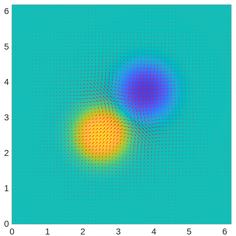
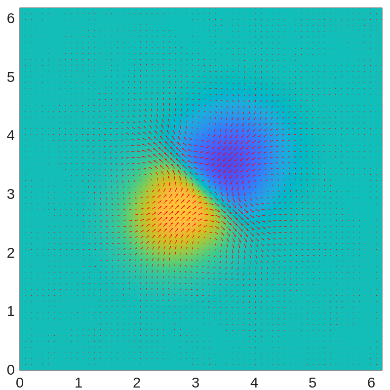
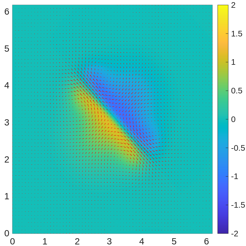
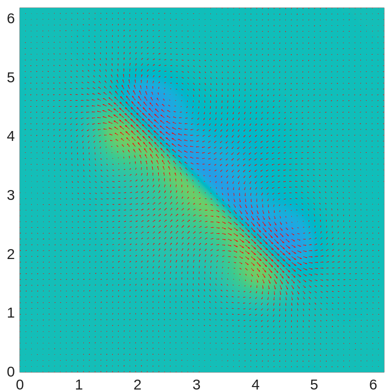
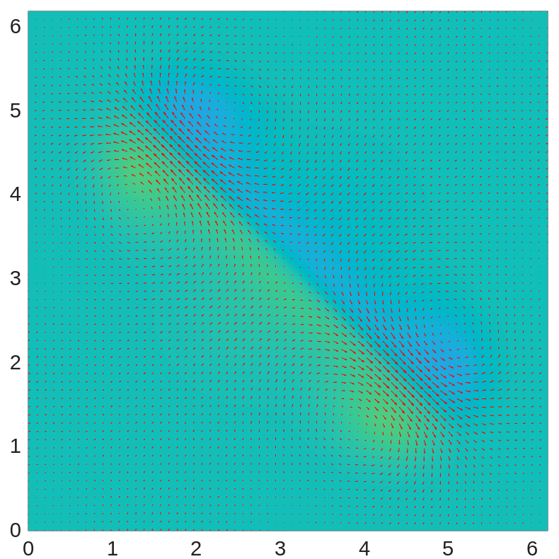
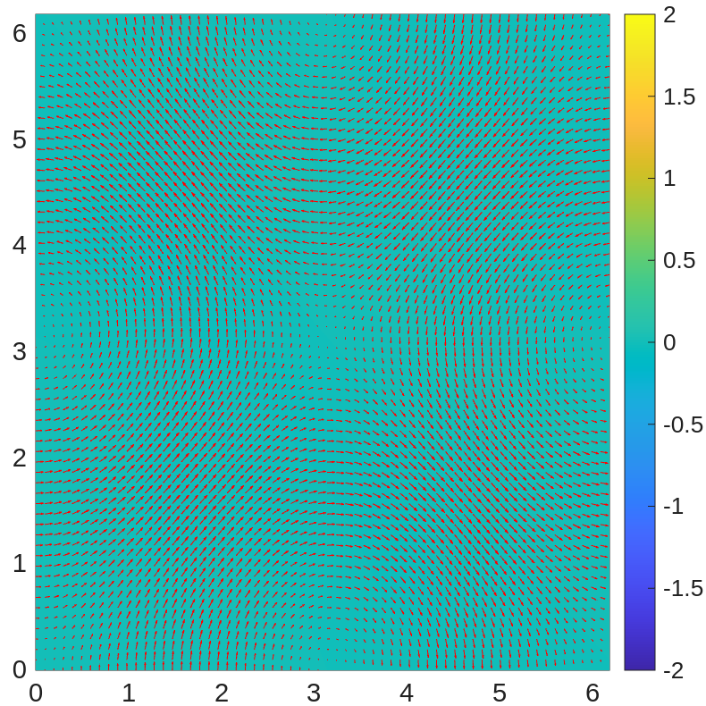
With time step $\Delta t=10^{-4}$ , in Figure 1, we plot the profiles of $p-n$ and the velocity field $\mathbf{u}$ at times $T=0.005$ , $0.025$ , $0.05$ , $0.075$ , $0.1$ , and $1$ . We observe that the positive and negative ions move toward each other and drag the fluid along with them. Later, the outflowing fluid between them prevents the ions from approaching each other further and carries the ions toward the corners. At the end of the computation, the fluid becomes almost electro-neutral.

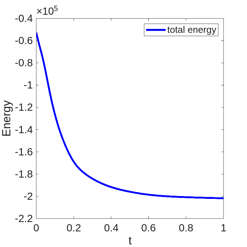
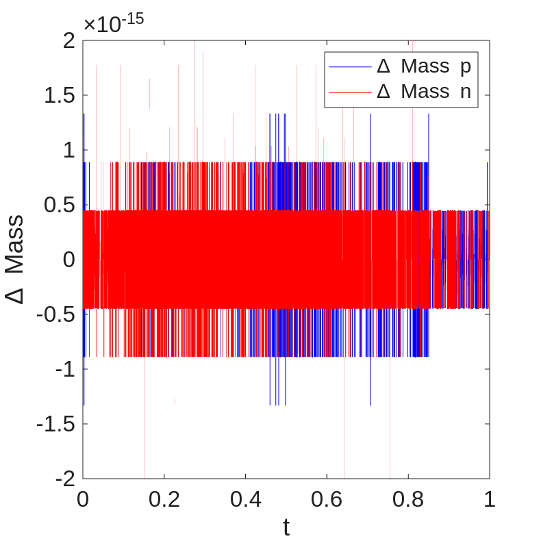
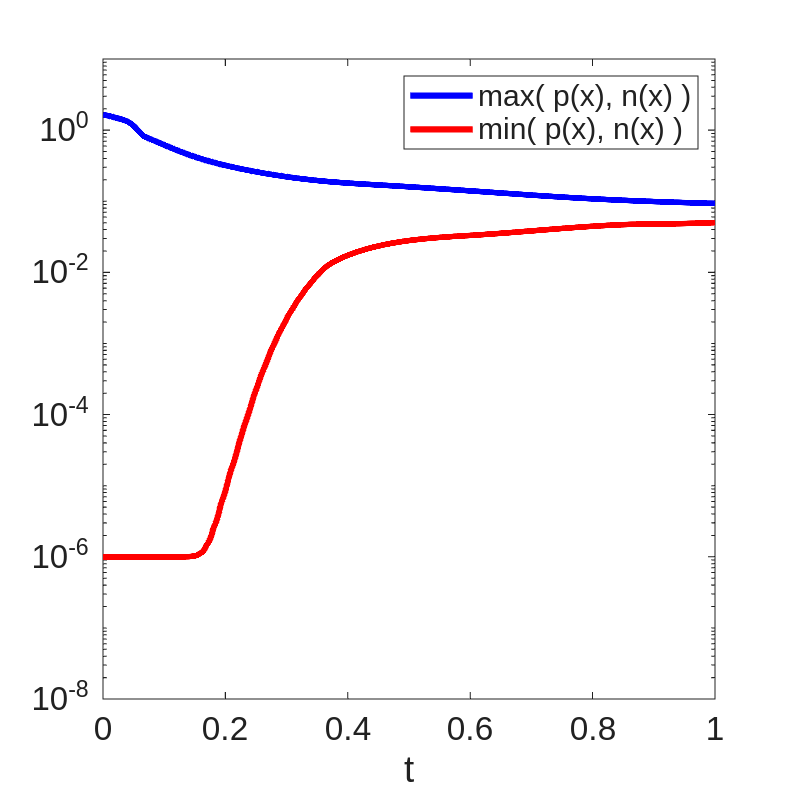
Refer to caption — Figure 1. Snapshots of $p-n$ and velocity field $\mathbf{u}$ at times $T=0.005$ , $0.025$ , $0.05$ , $0.075$ , $0.1$ , and $1$ .

We also examine the energy dissipation of the system in Figure 2(left), where the system energy is shown to be dissipative as we have proved. We plot the mass change for positive and negative ions in Figure 2(middle), showing that the mass of ions is preserved within machine precision. We also plot the minimum and maximum of $(p,n)$ in Figure 2(right), demonstrating that the ionic concentrations remain positive throughout the simulation.

6. Concluding Remarks

In this paper, we mainly consider numerical approximations for the PNP-NS system. Firstly, we give the results of unique solvability and regularity for the solution of PNP-NS system with suitable assumptions on initial conditions. To efficiently solve this coupled system, we propose a decoupled, mass-conserving, positivity-preserving and energy stable scheme which can also be unique solvable. Furthermore, we also carry out a rigorous error analysis for the fully discretized scheme, and derive optimal convergence results. The error analysis mainly depends on the $L^{\infty}$ bounds for the numerical solutions $n$ and $p$ , which are obtained by using a high-order asymptotic expansion for the PNP-NS system combing with a mathematical induction technique. We also present some numerical examples to validate the accuracy and stability of our decoupled scheme.

Appendix A Appendix

A.1. High order correction

Lemma A.1.

Let $(p,n,{\bf u})$ be the solution of the PNP-NS system (1.1)-(1.5) which satisfies the following properties:

(1)

The ionic concentrations are strictly positive

$p,n\geq\delta_{0}>0,$

(2)

The solution satisfies

\begin{array}[]{ll}&(\partial_{t}^{4}p,\partial_{t}^{4}n,\partial_{t}^{4}{\bf u})\in L^{\infty}(0,T;L^{2}(\Omega)),(\partial_{t}^{3}p,\partial_{t}^{3}n,\partial_{t}^{3}{\bf u})\in L^{\infty}(0,T;H^{k+1}(\Omega))\ (k\geq 2),\end{array}

then we can construct correction functions $(p_{\Delta t,i},n_{\Delta t,i},{\bf u}_{\Delta t,i},\phi_{\Delta t,i})(i=1,2)$ depending only on $(p,n,{\bf u},\psi)$ such that the supplementary fields $(\breve{p},\breve{n},\breve{{\bf u}},\breve{\phi},\breve{\mu},\breve{\nu},\breve{\psi})$ (defined by (4.1)) has higher order consistency truncation error(as defined in (4.5)-(4.9)):

\rvert\breve{\tau}^{m+1}_{p}(v_{N})\rvert,\rvert\breve{\tau}^{m+1}_{n}(v_{N})\rvert,\rvert\breve{\tau}^{m+1}_{{\bf u}}(v_{N})\rvert\leq C(\Delta t^{3}+N^{-k})\|v_{N}\|_{H^{1}}.

Moreover, with $\Delta t,\frac{1}{N}$ chosen small enough, we have

(1)

The supplementary functions are strictly positive

$\breve{p},\breve{n}\geq\delta_{0}^{*}>0,$
(2)

The supplementary functions satisfy

$(\breve{p},\breve{n},\breve{{\bf u}})\in L^{\infty}(0,T,W^{1,\infty}).$

Proof.

Let $(p^{m},n^{m},{\bf u}^{m},\phi^{m})$ be the $L^{2}$ -orthogonal projection of continuous solution $(p,n,{\bf u},\phi)(m\Delta t)$ onto $X_{N}\times X_{N}\times X_{N}^{2}\times X_{N}$ , as defined in (4). From Taylor expansion, the local truncation error may be written into two parts, time discretization error and spatial discretization error, we have

	$\displaystyle\langle\frac{p^{m+1}-p^{m}}{\Delta t},v_{N}\rangle-\langle p^{m}{\bf u}^{m},\nabla v_{N}\rangle+\langle p^{m}(1+2\Delta tp^{m})\nabla\mu^{m+1},\nabla v_{N}\rangle$
(A.1)		$\displaystyle\qquad=-\langle\Delta tf^{m+1}_{p,1}+\Delta t^{2}f^{m+1}_{p,2}+\mathcal{O}(\Delta t^{3})+g^{m+1}_{p},v_{N}\rangle,$
	$\displaystyle\langle\frac{n^{m+1}-n^{m}}{\Delta t},v_{N}\rangle-\langle n^{m}{\bf u}^{m},\nabla v_{N}\rangle+\langle n^{m}(1+2\Delta tn^{m})\nabla\nu^{m+1},\nabla v_{N}\rangle$
(A.2)		$\displaystyle\qquad=-\langle\Delta tf^{m+1}_{n,1}+\Delta t^{2}f^{m+1}_{n,2}+\mathcal{O}(\Delta t^{3})+g^{m+1}_{n},v_{N}\rangle,$
	$\displaystyle\langle\frac{R_{N}{\bf u}^{m+1}-{\bf u}^{m}}{\Delta t},v_{N}\rangle+\langle({\bf u}^{m}\cdot\nabla)R_{N}{\bf u}^{m+1},v_{N}\rangle+\langle\nabla R_{N}{\bf u}^{m+1},\nabla v_{N}\rangle+\langle\nabla\phi^{m},v_{N}\rangle$
(A.3)		$\displaystyle\quad+\langle p^{m}\nabla\mu^{m+1}+n^{m}\nabla\nu^{m+1},v_{N}\rangle=-\langle\Delta tf^{m+1}_{{\bf u},1}+\Delta t^{2}f^{m+1}_{{\bf u},2}+\mathcal{O}(\Delta t^{3})+g^{m+1}_{{\bf u}},v_{N}\rangle,$

where $(f_{p,i}^{m+1},f_{n,i}^{m+1},f_{{\bf u},i}^{m+1})_{i=1,2}$ are the temporal part of truncation error and $(g_{p}^{m+1},g_{n}^{m+1},g_{{\bf u}}^{m+1})$ are the spatial part of the truncation error. From Taylor expansion, we can compute

	$\displaystyle f_{p,1}$	$\displaystyle=\frac{1}{2}\frac{\partial^{2}}{\partial t^{2}}p+\nabla\cdot(\partial_{t}(p{\bf u}))-\nabla\cdot((\partial_{t}p-2p^{2})\nabla(\ln{p}+\psi)),$
	$\displaystyle f_{n,1}$	$\displaystyle=\frac{1}{2}\frac{\partial^{2}}{\partial t^{2}}n+\nabla\cdot(\partial_{t}(n{\bf u}))-\nabla\cdot((\partial_{t}n-2n^{2})\nabla(\ln{n}-\psi)),$
	$\displaystyle f_{{\bf u},1}$	$\displaystyle=\frac{1}{2}\frac{\partial^{2}}{\partial t^{2}}{\bf u}+\partial_{t}{\bf u}\cdot\nabla{\bf u}+\partial_{t}p\nabla(\ln{p}+\psi)+\partial_{t}n\nabla(\ln{n}-\psi);$

	$\displaystyle f_{p,2}$	$\displaystyle=-\frac{1}{6}\frac{\partial^{3}}{\partial t^{3}}p-\frac{1}{2}\nabla\cdot(\frac{\partial^{2}}{\partial t^{2}}(p{\bf u}))+\nabla\cdot\big{(}(\frac{1}{2}\frac{\partial^{2}}{\partial t^{2}}p-4p\partial_{t}p)\nabla(\ln{p}+\psi)\big{)}$
	$\displaystyle f_{n,2}$	$\displaystyle=-\frac{1}{6}\frac{\partial^{3}}{\partial t^{3}}n-\frac{1}{2}\nabla\cdot(\frac{\partial^{2}}{\partial t^{2}}(n{\bf u}))+\nabla\cdot\big{(}(\frac{1}{2}\frac{\partial^{2}}{\partial t^{2}}n-4n\partial_{t}n)\nabla(\ln{n}-\psi)\big{)}$
	$\displaystyle f_{{\bf u},2}$	$\displaystyle=-\frac{1}{6}\frac{\partial^{3}}{\partial t^{3}}{\bf u}-\frac{1}{2}\frac{\partial^{2}}{\partial t^{2}}{\bf u}\cdot\nabla{\bf u}-({\bf u}\cdot\nabla)\nabla\partial_{t}\phi-\Delta(\nabla\partial_{t}\phi)$
		$\displaystyle\quad-\frac{1}{2}\frac{\partial^{2}}{\partial t^{2}}p\nabla(\ln{p}+\psi)-\frac{1}{2}\frac{\partial^{2}}{\partial t^{2}}n\nabla(\ln{n}-\psi)$

and

	$\displaystyle\langle g_{p}^{m+1},v_{N}\rangle$	$\displaystyle\lesssim N^{-k}(\\|p_{t}\\|_{H^{k}}+\\|p{\bf u}\\|_{H^{k}}+\\|p\nabla(\ln{p}+\psi)\\|_{H^{k}})\big{(}(m+1)\Delta t\big{)}\\|v_{N}\\|_{H^{1}},$
	$\displaystyle\langle g_{n}^{m+1},v_{N}\rangle$	$\displaystyle\lesssim N^{-k}(\\|n_{t}\\|_{H^{k}}+\\|n{\bf u}\\|_{H^{k}}+\\|n\nabla(\ln{n}-\psi)\\|_{H^{k}})\big{(}(m+1)\Delta t\big{)}\\|v_{N}\\|_{H^{1}},$
	$\displaystyle\langle g_{{\bf u}}^{m+1},v_{N}\rangle$	$\displaystyle\lesssim N^{-k}\big{(}\\|{\bf u}_{t}\\|_{H^{k}}+\\|({\bf u}\cdot\nabla){\bf u}\\|_{H^{k}}+\\|\nabla{\bf u}\\|_{H^{k}}+\\|\nabla\psi\\|_{H^{k}}$
		$\displaystyle\quad\quad\quad+\\|p\nabla(\ln{p}+\psi)+n\nabla(\ln{n}-\psi\\|_{H^{k}}\big{)}\big{(}(m+1)\Delta t\big{)}\\|v_{N}\\|_{H^{1}}.$

Applying the regularity assumption (2), we have

(A.4)

\begin{split}&\partial_{t}^{2}f_{p,1}\in L^{\infty}(0,T;L^{2}(\Omega)),\ \partial_{t}f_{p,1}\in L^{\infty}(0,T;H^{k+1}(\Omega)),\\ &\partial_{t}^{2}f_{n,1}\in L^{\infty}(0,T;L^{2}(\Omega)),\ \partial_{t}f_{n,1}\in L^{\infty}(0,T;H^{k+1}(\Omega)),\\ &\partial_{t}^{2}f_{{\bf u},1}\in L^{\infty}(0,T;L^{2}(\Omega)),\ \partial_{t}f_{{\bf u},1}\in L^{\infty}(0,T;H^{k+1}(\Omega)),\end{split}

\langle g^{m+1}_{p,1},v_{N}\rangle,\langle g^{m+1}_{n,1},v_{N}\rangle,\langle g^{m+1}_{{\bf u},1},v_{N}\rangle\lesssim N^{-k}\|v_{N}\|_{H^{1}}.

With those $(f_{p,1},f_{n,1},f_{{\bf u},1})$ , we construct and solve the leading order temporal correction function $(p_{\Delta t,1},n_{\Delta t,1},{\bf u}_{\Delta t,1},\phi_{\Delta t,1})$ from the following equation:

	$\displaystyle\partial_{t}p_{\Delta t,1}$	$\displaystyle=\nabla\cdot(p\nabla(\frac{p_{\Delta t,1}}{p}+\psi_{\Delta t,1})+p_{\Delta t,1}\nabla(\ln{p}+\psi))$
(A.5)			$\displaystyle\quad-\nabla\cdot(p_{\Delta t,1}{\bf u}+p{\bf u}_{\Delta t,1})-f_{p,1},$
	$\displaystyle\partial_{t}n_{\Delta t,1}$	$\displaystyle=\nabla\cdot(n\nabla(\frac{n_{\Delta t,1}}{n}-\psi_{\Delta t,1})+n_{\Delta t,1}\nabla(\ln{n}-\psi))$
(A.6)			$\displaystyle\quad-\nabla\cdot(n_{\Delta t,1}{\bf u}+n{\bf u}_{\Delta t,1})-f_{n,1},$
(A.7)		$\displaystyle-\Delta\psi_{\Delta t,1}$	$\displaystyle=p_{\Delta t,1}-n_{\Delta t,1},$
	$\displaystyle\partial_{t}{\bf u}_{\Delta t,1}$	$\displaystyle=\Delta{\bf u}_{\Delta t,1}-\nabla\phi_{\Delta t,1}-({\bf u}\cdot\nabla){\bf u}_{\Delta t,1}-({\bf u}_{\Delta t,1}\cdot\nabla){\bf u}$
		$\displaystyle\qquad-p\nabla(\frac{p_{\Delta t,1}}{p}+\psi_{\Delta t,1})-p_{\Delta t,1}\nabla(\ln{p}+\psi)$
(A.8)			$\displaystyle\qquad-n\nabla(\frac{n_{\Delta t,1}}{n}-\psi_{\Delta t,1})-n_{\Delta t,1}\nabla(\ln{n}-\psi)-f_{{\bf u},1},$
(A.9)		$\displaystyle\nabla\cdot{\bf u}_{\Delta t,1}$	$\displaystyle=0,$

subject to the periodic boundary condition and zero initial condition. The PDE system (A.5)-(A.9) is very similar to the PNP-NS system (1.1)-(1.5), and the existence of solution could be established similarly. Moreover, given the regularity of $(p,n,{\bf u},\phi)$ and $(f_{p,1},f_{n,1},f_{{\bf u},1})$ in (A.4), the solution satisfies

(A.10)

(\partial_{t}^{3}p_{\Delta t,1},\partial_{t}^{3}n_{\Delta t,1},\partial_{t}^{3}{\bf u}_{\Delta t,1})\in L^{\infty}(0,T,L^{2}(\Omega)),\ (\partial_{t}^{2}p_{\Delta t,1},\partial_{t}^{2}n_{\Delta t,1},\partial_{t}^{2}{\bf u}_{\Delta t,1})\in L^{\infty}(0,T,H^{k+1}(\Omega)).

The discretization of the above system implies that

	$\displaystyle\langle-f^{m+1}_{p,1},v_{N}\rangle$	$\displaystyle=\langle\frac{p^{m+1}_{\Delta t,1}-p^{m}_{\Delta t,1}}{\Delta t},v_{N}\rangle-\langle p^{m}_{\Delta t,1}{\bf u}^{m}+p^{m}{\bf u}^{m}_{\Delta t,1},\nabla v_{N}\rangle$
		$\displaystyle\quad+\langle p^{m}(1+2\Delta tp^{m})\nabla(\frac{p^{m+1}_{\Delta t,1}}{p^{m+1}}+\psi^{m+1}_{\Delta t,1})$
		$\displaystyle\quad\quad+p^{m}_{\Delta t,1}(1+2\Delta tp^{m})\nabla(\ln{p^{m+1}+\psi^{m+1}}),\nabla v_{N}\rangle$
(A.11)			$\displaystyle\quad-\langle\Delta tf_{p_{\Delta t,1},1}^{m+1}+g_{p_{\Delta t,1}}^{m+1}+\mathcal{O}(\Delta t^{2}),v_{N}\rangle,$
	$\displaystyle\langle-f^{m+1}_{n,1},v_{N}\rangle$	$\displaystyle=\langle\frac{n^{m+1}_{\Delta t,1}-n^{m}_{\Delta t,1}}{\Delta t},v_{N}\rangle-\langle n^{m}_{\Delta t,1}{\bf u}^{m}+n^{m}{\bf u}^{m}_{\Delta t,1},\nabla v_{N}\rangle$
		$\displaystyle\quad+\langle n^{m}(1+2\Delta tn^{m})\nabla(\frac{n^{m+1}_{\Delta t,1}}{n^{m+1}}-\psi^{m+1}_{\Delta t,1})$
		$\displaystyle\quad\quad+n^{m}_{\Delta t,1}(1+2\Delta tn^{m})\nabla(\ln{n^{m+1}-\psi^{m+1}}),\nabla v_{N}\rangle$
(A.12)			$\displaystyle\quad-\langle\Delta tf_{n_{\Delta t,1},1}^{m+1}+g_{n_{\Delta t,1}}^{m+1}+\mathcal{O}(\Delta t^{2}),v_{N}\rangle,$
	$\displaystyle\langle-f^{m+1}_{{\bf u},1},v_{N}\rangle$	$\displaystyle=\langle\frac{R_{N}{\bf u}^{m+1}_{\Delta t,1}-{\bf u}^{m}_{\Delta t,1}}{\Delta t},v_{N}\rangle+\langle\nabla R_{N}{\bf u}^{m+1}_{\Delta t,1},\nabla v_{N}\rangle+\langle\nabla\phi^{m}_{\Delta t,1},v_{N}\rangle$
		$\displaystyle\quad+\langle({\bf u}^{m}\cdot\nabla)R_{N}{\bf u}^{m+1}_{\Delta t,1}+({\bf u}^{m}_{\Delta t,1}\cdot\nabla)R_{N}{\bf u}^{m+1},v_{N}\rangle$
		$\displaystyle\quad+\langle p^{m}\nabla(\frac{p^{m+1}_{\Delta t,1}}{p^{m+1}}+\psi^{m+1}_{\Delta t,1})+p^{m}_{\Delta t,1}\nabla(\ln{p^{m+1}}+\psi^{m+1}),v_{N}\rangle$
		$\displaystyle\quad+\langle n^{m}\nabla(\frac{n^{m+1}_{\Delta t,1}}{n^{m+1}}-\psi^{m+1}_{\Delta t,1})+n^{m}_{\Delta t,1}\nabla(\ln{n^{m+1}}-\psi^{m+1}),v_{N}\rangle$
(A.13)			$\displaystyle\quad-\langle\Delta tf_{{\bf u}_{\Delta t,1},1}^{m+1}+g_{{\bf u}_{\Delta t,1}}^{m+1}+\mathcal{O}(\Delta t^{2}),v_{N}\rangle,$
(A.14)		$\displaystyle\langle\nabla\psi^{m}_{\Delta t,1},\nabla v_{N}$	$\displaystyle\rangle=\langle p^{m}_{\Delta t,1}-n^{m}_{\Delta t,1},v_{N}\rangle,$
(A.15)		$\displaystyle\langle{\bf u}^{m}_{\Delta t,1},\nabla v_{N}$	$\displaystyle\rangle=0.$

where $(f_{p_{\Delta t,1},1},f_{n_{\Delta t,1},1},f_{{\bf u}_{\Delta t,1},1})$ and $(g_{p_{\Delta t,1}},g_{n_{\Delta t,1}},g_{{\bf u}_{\Delta t,1}})$ are the temporal part and spatial part of the truncation error, from Taylor expansion, we have

	$\displaystyle f_{p_{\Delta t,1},1}$	$\displaystyle=\frac{1}{2}\frac{\partial^{2}}{\partial t^{2}}p_{\Delta t,1}+\nabla\cdot\big{(}\partial_{t}(p_{\Delta t,1}{\bf u}+p{\bf u}_{\Delta t,1})\big{)}-\nabla\cdot\big{(}(\partial_{t}p-2p^{2})\nabla(\frac{p_{\Delta t,1}}{p}+\psi_{\Delta t,1})\big{)}$
		$\displaystyle\quad-\nabla\cdot\big{(}(\partial_{t}p-4p_{\Delta t,1}p)\nabla(\ln{p}+\psi)\big{)}$
	$\displaystyle f_{n_{\Delta t,1},1}$	$\displaystyle=\frac{1}{2}\frac{\partial^{2}}{\partial t^{2}}n_{\Delta t,1}+\nabla\cdot\big{(}\partial_{t}(n_{\Delta t,1}{\bf u}+n{\bf u}_{\Delta t,1})\big{)}-\nabla\cdot\big{(}(\partial_{t}n-2n^{2})\nabla(\frac{n_{\Delta t,1}}{n}-\psi_{\Delta t,1})\big{)}$
		$\displaystyle\quad-\nabla\cdot\big{(}(\partial_{t}n-4n_{\Delta t,1}n)\nabla(\ln{n}-\psi)\big{)}$
	$\displaystyle f_{{\bf u}_{\Delta t,1},1}$	$\displaystyle=\frac{1}{2}\frac{\partial^{2}}{\partial t^{2}}{\bf u}_{\Delta t,1}+(\partial_{t}{\bf u}\cdot\nabla){\bf u}_{\Delta t,1}+(\partial_{t}{\bf u}_{\Delta t,1}\cdot\nabla){\bf u}$
		$\displaystyle\quad+\partial_{t}p\nabla(\frac{p_{\Delta t,1}}{p}+\psi_{\Delta t,1})+\partial_{t}p_{\Delta t,1}\nabla(\ln{p+\psi})$
		$\displaystyle\quad+\partial_{t}n\nabla(\frac{n_{\Delta t,1}}{n}-\psi_{\Delta t,1})+\partial_{t}n_{\Delta t,1}\nabla(\ln{n-\psi})$

and

\begin{array}[]{ll}\langle g_{p,\Delta t,1}^{m+1},v_{N}\rangle&\lesssim N^{-k}\big{(}\|\partial_{t}p_{\Delta t,1}\|_{L^{\infty}_{t}H^{k}}+\|p_{\Delta t,1}\|_{L^{\infty}_{t}H^{k+1}}+\|p\nabla\psi_{\Delta t,1}\|_{L^{\infty}_{t}H^{k}}\vskip 3.00003pt\\ &\quad+\|p_{\Delta t,1}\nabla p\|_{L^{\infty}_{t}H^{k}}+\|f_{p,1}\|_{L^{\infty}_{t}H^{k}}\big{)}\|v_{N}\|_{H^{1}}\vskip 5.0pt,\\ \langle g_{n,\Delta t,1}^{m+1},v_{N}\rangle&\lesssim N^{-k}\big{(}\|\partial_{t}n_{\Delta t,1}\|_{L^{\infty}_{t}H^{k}}+\|n_{\Delta t,1}\|_{L^{\infty}_{t}H^{k+1}}+\|n\nabla\psi_{\Delta t,1}\|_{L^{\infty}_{t}H^{k}}\vskip 3.00003pt\\ &\quad+\|p_{\Delta t,1}\nabla p\|_{L^{\infty}_{t}H^{k}}+\|f_{p,1}\|_{L^{\infty}_{t}H^{k}}\big{)}\|v_{N}\|_{H^{1}}\vskip 5.0pt,\\ \langle g_{{\bf u},\Delta t,1}^{m+1},v_{N}\rangle&\lesssim N^{-k}\big{(}\|\partial_{t}{\bf u}_{\Delta t,1}\|_{L^{\infty}_{t}H^{k}}+\|\nabla{\bf u}_{\Delta t,1}\|_{L^{\infty}_{t}H^{k}}+\|\nabla\psi_{\Delta t,1}\|_{L^{\infty}_{t}H^{k}}\vskip 3.00003pt\\ &\quad+\|({\bf u}_{\Delta t,1}\cdot\nabla){\bf u}\|_{L^{\infty}_{t}H^{k}}+\|({\bf u}\cdot\nabla){\bf u}_{\Delta t,1}\|_{L^{\infty}_{t}H^{k}}+\|p\nabla\psi_{\Delta t,1}\|_{H^{k}}+\|p_{\Delta t,1}\nabla\psi_{\Delta t,1}\|_{L^{\infty}_{t}H^{k}}\vskip 3.00003pt\\ &\quad+\|n\nabla\psi_{\Delta t,1}\|_{L^{\infty}_{t}H^{k}}+\|n_{\Delta t,1}\nabla\psi_{\Delta t,1}\|_{L^{\infty}_{t}H^{k}}+\|f_{{\bf u},1}\|_{L^{\infty}_{t}H^{k}}\big{)}\|v_{N}\|_{H^{1}}.\end{array}

From the regularity result in (A.4) and (A.10), we have

\langle g^{m+1}_{p,2},v_{N}\rangle,\langle g^{m+1}_{n,2},v_{N}\rangle,\langle g^{m+1}_{{\bf u},2},v_{N}\rangle\lesssim N^{-k}\|v_{N}\|_{H^{1}}.

Combining (A.1)-(A.3) and (A.11)-(A.13) leads to the second order temporal local truncation error for $\breve{p}_{1}=\Pi_{N}(p+\Delta tp_{\Delta t,1}),\ \breve{n}_{1}=\Pi_{N}(n+\Delta tn_{\Delta t,1}),\ \breve{{\bf u}}_{1}=\Pi_{N}({\bf u}+\Delta t{\bf u}_{\Delta t,1}),\ \breve{\phi}_{1}=\Pi_{N}(\phi+\Delta t\phi_{\Delta t,1})$ :

	$\displaystyle\langle\frac{\breve{p}_{1}^{m+1}-\breve{p}_{1}^{m}}{\Delta t},v_{N}\rangle-\langle\breve{p}_{1}^{m}\breve{{\bf u}}_{1}^{m},\nabla v_{N}\rangle+\langle\breve{p}_{1}^{m}(1+2\Delta t\breve{p}_{1}^{m})\nabla\breve{\mu}_{1}^{m+1},\nabla v_{N}\rangle$
(A.16)		$\displaystyle\qquad=-\langle\Delta t^{2}f^{m+1}_{\breve{p}_{1},2}+\mathcal{O}(\Delta t^{3})+\mathcal{O}(N^{-k}),v_{N}\rangle,$
	$\displaystyle\langle\frac{\breve{n}_{1}^{m+1}-\breve{n}_{1}^{m}}{\Delta t},v_{N}\rangle-\langle\breve{n}_{1}^{m}\breve{{\bf u}}_{1}^{m},\nabla v_{N}\rangle+\langle\breve{n}_{1}^{m}(1+2\Delta t\breve{n}_{1}^{m})\nabla\breve{\nu}_{1}^{m+1},\nabla v_{N}\rangle$
(A.17)		$\displaystyle\qquad=-\langle\Delta t^{2}f^{m+1}_{\breve{n}_{1},2}+\mathcal{O}(\Delta t^{3})+\mathcal{O}(N^{-k}),v_{N}\rangle,$
	$\displaystyle\langle\frac{R_{N}\breve{{\bf u}}_{1}^{m+1}-\breve{{\bf u}}_{1}^{m}}{\Delta t},v_{N}\rangle+\langle(\breve{{\bf u}}_{1}^{m}\cdot\nabla)R_{N}\breve{{\bf u}}_{1}^{m+1},v_{N}\rangle+\langle\nabla R_{N}\breve{{\bf u}}_{1}^{m+1},\nabla v_{N}\rangle+\langle\nabla\breve{\phi}_{1}^{m},v_{N}\rangle$
(A.18)		$\displaystyle+\langle\breve{p}_{1}^{m}\nabla\breve{\mu}_{1}^{m+1}+\breve{n}_{1}^{m}\nabla\breve{\nu}_{1}^{m+1},v_{N}\rangle=-\langle\Delta t^{2}f^{m+1}_{\breve{{\bf u}}_{1},2}+\mathcal{O}(\Delta t^{3})+\mathcal{O}(N^{-k}),v_{N}\rangle,$

where

	$\displaystyle\breve{\psi}_{1}=\Pi_{N}[(-\Delta)^{-1}(\breve{p}_{1}-\breve{n}_{1})],$
	$\displaystyle\breve{\mu}_{1}=\Pi_{N}(\ln{\breve{p}_{1}}+\breve{\psi}_{1}),\ \breve{\nu}_{1}=\Pi_{N}(\ln{\breve{n}_{1}}-\breve{\psi}_{1}),$

and

	$\displaystyle f_{\breve{p}_{1},2}$	$\displaystyle=f_{p,2}+f_{p_{\Delta t,1},1}+\nabla\cdot(p_{\Delta t,1}{\bf u}_{\Delta t,1})-\nabla\cdot(2pp_{\Delta t,1}\nabla(\ln{p}+\psi))$
		$\displaystyle\quad-\nabla\cdot(p\nabla(\frac{p_{\Delta t,1}}{p})^{2})+\nabla\cdot(p_{\Delta t,1}\nabla(\frac{p_{\Delta t,1}}{p}+\psi)),$
	$\displaystyle f_{\breve{n}_{1},2}$	$\displaystyle=f_{n,2}+f_{n_{\Delta t,1},1}+\nabla\cdot(n_{\Delta t,1}{\bf u}_{\Delta t,1})-\nabla\cdot(2nn_{\Delta t,1}\nabla(\ln{n}-\psi))$
		$\displaystyle\quad-\nabla\cdot(n\nabla(\frac{n_{\Delta t,1}}{n})^{2})-\nabla\cdot(n_{\Delta t,1}\nabla(\frac{n_{\Delta t,1}}{n}-\psi)),$
	$\displaystyle f_{\breve{{\bf u}}_{1},2}$	$\displaystyle=f_{{\bf u},2}+f_{{\bf u}_{\Delta t,1},1}+({\bf u}_{\Delta t,1}\cdot\nabla){\bf u}_{\Delta t,1}$
		$\displaystyle\quad+p_{\Delta t,1}\nabla(\frac{p_{\Delta t,1}}{p}+\psi_{\Delta t,1})-p\nabla((\frac{p_{\Delta t,1}}{p})^{2})$
		$\displaystyle\quad+n_{\Delta t,1}\nabla(\frac{n_{\Delta t,1}}{n}-\psi_{\Delta t,1})-n\nabla((\frac{n_{\Delta t,1}}{n})^{2}).$

Since $(p_{\Delta t,1},n_{\Delta t,1})$ are bounded, we may choose $\Delta t,\frac{1}{N}$ so small that $\breve{p}_{1},\breve{n}_{1}>\frac{\delta_{0}}{2}>0$ . And $(f_{\breve{p}_{1},2}^{m+1},f_{\breve{n}_{1},2}^{m+1},f_{\breve{{\bf u}}_{1},2}^{m+1})$ are the temporal projection of functions $(f_{\breve{p}_{1},2},f_{\breve{n}_{1},2},f_{\breve{{\bf u}}_{1},2})$ onto $X_{N}\times X_{N}\times X_{N}^{2}$ . From (2) (A.10) we have

(\partial_{t}f_{\breve{p}_{1},2},\partial_{t}f_{\breve{n}_{1},2},\partial_{t}f_{\breve{{\bf u}}_{1},2})\in L^{\infty}(0,T;L^{2}(\Omega)),\ (f_{\breve{p}_{1},2},f_{\breve{n}_{1},2},f_{\breve{{\bf u}}_{1},2})\in L^{\infty}(0,T;H^{k+1}(\Omega)).

Similarly, the next order temporal correction function $(p_{\Delta t,2},n_{\Delta t,2},{\bf u}_{\Delta t,2},\phi_{\Delta t,2})$ is given by the following system:

	$\displaystyle\partial_{t}p_{\Delta t,2}=\nabla\cdot(\breve{p}_{1}\nabla(\frac{p_{\Delta t,2}}{\breve{p}_{1}}+\psi_{\Delta t,2})+p_{\Delta t,2}\nabla(\ln{\breve{p}_{1}}+\breve{\psi}_{1}))$
(A.19)		$\displaystyle\qquad-\nabla\cdot(p_{\Delta t,2}\breve{{\bf u}}_{1}+\breve{p}_{1}{\bf u}_{\Delta t,2})-f_{\breve{p}_{1},2},$
	$\displaystyle\partial_{t}n_{\Delta t,2}=\nabla\cdot(\breve{n}_{1}\nabla(\frac{n_{\Delta t,2}}{\breve{n}_{1}}-\psi_{\Delta t,2})+n_{\Delta t,2}\nabla(\ln{\breve{n}_{1}}-\breve{\psi}_{1}))$
(A.20)		$\displaystyle\qquad-\nabla\cdot(n_{\Delta t,2}\breve{{\bf u}}_{1}+\breve{n}_{1}{\bf u}_{\Delta t,2})-f_{\breve{n}_{1},2},$
(A.21)		$\displaystyle-\Delta\psi_{\Delta t,2}=p_{\Delta t,2}-n_{\Delta t,2},$
	$\displaystyle\partial_{t}{\bf u}_{\Delta t,2}=\Delta{\bf u}_{\Delta t,2}-\nabla\phi_{\Delta t,2}-(\breve{{\bf u}}_{1}\cdot\nabla){\bf u}_{\Delta t,2}-({\bf u}_{\Delta t,2}\cdot\nabla)\breve{{\bf u}}_{1}$
	$\displaystyle\qquad-\breve{p}_{1}\nabla(\frac{p_{\Delta t,2}}{\breve{p}_{1}}+\psi_{\Delta t,2})-p_{\Delta t,2}\nabla(\ln{\breve{p}_{1}}+\breve{\psi}_{1})$
(A.22)		$\displaystyle\qquad-\breve{n}_{1}\nabla(\frac{n_{\Delta t,2}}{\breve{n}_{1}}-\psi_{\Delta t,2})-n_{\Delta t,2}\nabla(\ln{\breve{n}_{1}}-\breve{\psi}_{1})-f_{\breve{{\bf u}}_{1},2},$
(A.23)		$\displaystyle\nabla\cdot\breve{{\bf u}}_{\Delta t,2}=0.$

subject to the periodic boundary condition and zero initial condition. Then we have

(\partial_{t}^{2}p_{\Delta t,2},\partial_{t}^{2}n_{\Delta t,2},\partial_{t}^{2}{\bf u}_{\Delta t,2})\in L^{\infty}(0,T,L^{2}(\Omega)),\ (\partial_{t}p_{\Delta t,2},\partial_{t}n_{\Delta t,2},\partial_{t}{\bf u}_{\Delta t,2})\in L^{\infty}(0,T,H^{k+1}(\Omega)).

The discretization of the above system implies that

	$\displaystyle\langle-f^{m+1}_{\breve{p}_{1},2},v_{N}\rangle$	$\displaystyle=\langle\frac{p^{m+1}_{\Delta t,2}-p^{m}_{\Delta t,2}}{\Delta t},v_{N}\rangle-\langle p^{m}_{\Delta t,2}\breve{{\bf u}}_{1}^{m}+\breve{p}_{1}^{m}{\bf u}^{m}_{\Delta t,2},\nabla v_{N}\rangle$
		$\displaystyle\quad+\langle\breve{p}^{m}_{1}(1+2\Delta t\breve{p}^{m}_{1})\nabla(\frac{p^{m+1}_{\Delta t,2}}{\breve{p}^{m+1}_{1}}+\psi^{m+1}_{\Delta t,2})$
		$\displaystyle\quad+p^{m}_{\Delta t,2}(1+4\Delta t\breve{p}^{m}_{1})\nabla(\ln{\breve{p}^{m+1}_{1}+\breve{\psi}^{m+1}_{1}}),\nabla v_{N}\rangle$
(A.24)			$\displaystyle\quad+\mathcal{O}(\Delta t)+\mathcal{O}(N^{-k}),$
	$\displaystyle\langle-f^{m+1}_{\breve{n}_{1},2},v_{N}\rangle$	$\displaystyle=\langle\frac{n^{m+1}_{\Delta t,2}-n^{m}_{\Delta t,2}}{\Delta t},v_{N}\rangle-\langle n^{m}_{\Delta t,2}\breve{{\bf u}}_{1}^{m}+\breve{n}^{m}_{1}{\bf u}^{m}_{\Delta t,2},\nabla v_{N}\rangle$
		$\displaystyle\quad+\langle\breve{n}^{m}_{1}(1+2\Delta t\breve{n}^{m}_{1})\nabla(\frac{n^{m+1}_{\Delta t,2}}{\breve{n}^{m+1}_{1}}-\psi^{m+1}_{\Delta t,2})$
		$\displaystyle\quad+n^{m}_{\Delta t,2}(1+4\Delta t\breve{n}_{1}^{m})\nabla(\ln{\breve{n}_{1}^{m+1}-\breve{\psi}_{1}^{m+1}}),\nabla v_{N}\rangle$
(A.25)			$\displaystyle\quad+\mathcal{O}(\Delta t)+\mathcal{O}(N^{-k}),$
	$\displaystyle\langle-f^{m+1}_{\breve{{\bf u}}_{1},2},v_{N}\rangle$	$\displaystyle=\langle\frac{R_{N}{\bf u}^{m+1}_{\Delta t,2}-{\bf u}^{m}_{\Delta t,2}}{\Delta t},v_{N}\rangle+\langle\nabla R_{N}{\bf u}^{m+1}_{\Delta t,2},\nabla v_{N}\rangle+\langle\nabla\phi^{m}_{\Delta t,2},v_{N}\rangle$
		$\displaystyle\quad+\langle(\breve{{\bf u}}^{m}_{1}\cdot\nabla)R_{N}{\bf u}^{m+1}_{\Delta t,2}+({\bf u}^{m}_{\Delta t,2}\cdot\nabla)R_{N}\breve{{\bf u}}_{1}^{m+1},v_{N}\rangle$
		$\displaystyle\quad+\langle\breve{p}_{1}^{m}\nabla(\frac{p^{m+1}_{\Delta t,2}}{\breve{p}_{1}^{m+1}}+\psi^{m+1}_{\Delta t,2})+p^{m}_{\Delta t,2}\nabla(\ln{\breve{p}_{1}^{m+1}}+\breve{\psi}_{1}^{m+1}),v_{N}\rangle$
		$\displaystyle\quad+\langle\breve{n}_{1}^{m}\nabla(\frac{n^{m+1}_{\Delta t,2}}{\breve{n}_{1}^{m+1}}-\psi^{m+1}_{\Delta t,2})+n^{m}_{\Delta t,2}\nabla(\ln{\breve{n}_{1}^{m+1}}-\breve{\psi}_{1}^{m+1}),v_{N}\rangle$
(A.26)			$\displaystyle\quad+\mathcal{O}(\Delta t)+\mathcal{O}(N^{-k}),$
(A.27)		$\displaystyle\langle\nabla\psi^{m}_{\Delta t,2},\nabla v_{N}$	$\displaystyle\rangle=\langle p^{m}_{\Delta t,2}-n^{m}_{\Delta t,2},v_{N}\rangle,$
(A.28)		$\displaystyle\langle{\bf u}^{m}_{\Delta t,2},\nabla v_{N}$	$\displaystyle\rangle=0.$

Finally, a combination of (A.16)-(A.18) and (A.24)-(A.26) yields the third order temporal truncation error for $(\breve{p},\breve{n},\breve{{\bf u}},\breve{\phi})$ :

	$\displaystyle\langle\frac{\breve{p}^{m+1}-\breve{p}^{m}}{\Delta t},v_{N}\rangle-\langle\breve{p}^{m}\breve{{\bf u}}^{m},\nabla v_{N}\rangle+\langle\breve{p}^{m}(1+2\Delta t\breve{p}^{m})\nabla\breve{\mu}^{m+1},\nabla v_{N}\rangle=\tau^{m+1}_{p}(v_{N}),$
	$\displaystyle\langle\frac{\breve{n}^{m+1}-\breve{n}^{m}}{\Delta t},v_{N}\rangle-\langle\breve{n}^{m}\breve{{\bf u}}^{m},\nabla v_{N}\rangle+\langle\breve{n}^{m}(1+2\Delta tn^{m})\nabla\breve{\nu}^{m+1},\nabla v_{N}\rangle=\tau^{m+1}_{n}(v_{N}),$
	$\displaystyle\langle\frac{R_{N}\breve{{\bf u}}^{m+1}-\breve{{\bf u}}^{m}}{\Delta t},v_{N}\rangle+\langle(\breve{{\bf u}}^{m}\cdot\nabla)R_{N}\breve{{\bf u}}^{m+1},v_{N}\rangle+\langle\nabla R_{N}\breve{{\bf u}}^{m+1},\nabla v_{N}\rangle+\langle\nabla\breve{\phi}^{m},v_{N}\rangle$
	$\displaystyle\quad+\langle\breve{p}^{m}\nabla\breve{\mu}^{m+1}+\breve{n}^{m}\nabla\breve{\nu}^{m+1},v_{N}\rangle=\tau^{m+1}_{{\bf u}}(v_{N}),$

where

\breve{\tau}^{m+1}_{p}(v_{N}),\breve{\tau}^{m+1}_{n}(v_{N}),\breve{\tau}^{m+1}_{{\bf u}}(v_{N})\leq C(\Delta t^{3}+N^{-k})\|v_{N}\|_{H^{1}}.

Since $(p_{\Delta t,2},n_{\Delta t,2})$ are bounded, we may find $\Delta t,\frac{1}{N}$ so small that $\breve{p},\breve{n}>\delta_{0}^{*}\triangleq\frac{\delta_{0}}{4}>0$ . Moreover, given the regularity of $(p_{\Delta t,i},n_{\Delta t,i},{\bf u}_{\Delta t,i})(i=1,2)$ , we have

(\breve{p},\breve{n},\breve{{\bf u}})\in L^{\infty}(0,T,W^{1,\infty}(\Omega)).

∎

Remark 3.

Since we set the initial data of our modified solution to be the same as the initial data of the exact solution, i.e. $(\breve{p},\breve{n},\breve{{\bf u}},\breve{\phi})(\cdot,t=0)=(\Pi_{N}p,\Pi_{N}n,\Pi_{N}{\bf u},\Pi_{N}\phi)(\cdot,t=0)$ , we will assume trivial initial data

(A.29)

(p_{\Delta t,i},n_{\Delta t,i},{\bf u}_{\Delta t,i},\phi_{\Delta t,i})(\cdot,t=0)={\bf 0},

for $i=1,2$ in (A.5)-(A.9) and (A.19)-(A.23).

References

[1] Martin Z Bazant and Todd M Squires. Induced-charge electrokinetic phenomena. Current Opinion in Colloid & Interface Science, 15(3):203–213, 2010.
[2] Wenbin Chen, Cheng Wang, Xiaoming Wang, and Steven M Wise. Positivity-preserving, energy stable numerical schemes for the cahn-hilliard equation with logarithmic potential. Journal of Computational Physics: X, 3:100031, 2019.
[3] Qing Cheng and Jie Shen. A new lagrange multiplier approach for constructing structure preserving schemes, I. positivity preserving. Computer Methods in Applied Mechanics and Engineering, 391:114585, 2022.
[4] Qing Cheng and Jie Shen. A new lagrange multiplier approach for constructing structure preserving schemes, II. bound preserving. SIAM Journal on Numerical Analysis, 60(3):970–998, 2022.
[5] Peter Constantin and Mihaela Ignatova. On the Nernst–Planck–Navier–Stokes system. Archive for Rational Mechanics and Analysis, 232(3):1379–1428, 2019.
[6] Jie Ding, Zhongming Wang, and Shenggao Zhou. Positivity preserving finite difference methods for poisson–nernst–planck equations with steric interactions: Application to slit-shaped nanopore conductance. Journal of Computational Physics, 397:108864, 2019.
[7] Qiang Du, Lili Ju, Xiao Li, and Zhonghua Qiao. Maximum bound principles for a class of semilinear parabolic equations and exponential time-differencing schemes. SIAM Review, 63(2):317–359, 2021.
[8] Allen Flavell, Michael Machen, Bob Eisenberg, Julienne Kabre, Chun Liu, and Xiaofan Li. A conservative finite difference scheme for Poisson–Nernst–Planck equations. Journal of Computational Electronics, 13(1):235–249, 2014.
[9] Huajun Gong, Changyou Wang, and Xiaotao Zhang. Partial regularity of suitable weak solutions of the Navier–Stokes–Planck–Nernst–Poisson equation. SIAM Journal on Mathematical Analysis, 53(3):3306–3337, 2021.
[10] Jean-Luc Guermond, Peter Minev, and Jie Shen. An overview of projection methods for incompressible flows. Computer Methods in Applied Mechanics and Engineering, 195(44-47):6011–6045, 2006.
[11] Jean-Luc Guermond and Luigi Quartapelle. On stability and convergence of projection methods based on pressure poisson equation. International Journal for Numerical Methods in Fluids, 26(9):1039–1053, 1998.
[12] Jean-Luc Guermond and Luigi Quartapelle. On the approximation of the unsteady Navier–Stokes equations by finite element projection methods. Numerische mathematik, 80(2):207–238, 1998.
[13] Jingwei Hu and Xiaodong Huang. A fully discrete positivity-preserving and energy-dissipative finite difference scheme for Poisson–Nernst–Planck equations. Numerische Mathematik, 145(1):77–115, 2020.
[14] Fukeng Huang and Jie Shen. Bound/positivity preserving and energy stable SAV schemes for dissipative systems: Applications to Keller-Segel and Poisson-Nernst-Planck equations. SIAM Journal on Scientific Computing, 43(3), 2021.
[15] Buyang Li, Jiang Yang, and Zhi Zhou. Arbitrarily high-order exponential cut-off methods for preserving maximum principle of parabolic equations. SIAM Journal on Scientific Computing, 42(6):A3957–A3978, 2020.
[16] Hao Li, Shusen Xie, and Xiangxiong Zhang. A high order accurate bound-preserving compact finite difference scheme for scalar convection diffusion equations. SIAM Journal on Numerical Analysis, 56(6):3308–3345, 2018.
[17] Hao Li and Xiangxiong Zhang. On the monotonicity and discrete maximum principle of the finite difference implementation of $C^{0}$ - $Q^{2}$ finite element method. Numerische Mathematik, 145(2):437–472, 2020.
[18] Chun Liu, Cheng Wang, Steven Wise, Xingye Yue, and Shenggao Zhou. A positivity-preserving, energy stable and convergent numerical scheme for the Poisson-Nernst-Planck system. Mathematics of Computation, 90(331):2071–2106, 2021.
[19] Chun Liu, Cheng Wang, Steven M Wise, Xingye Yue, and Shenggao Zhou. A second order accurate, positivity preserving numerical method for the poisson–nernst–planck system and its convergence analysis. Journal of scientific computing, 97(1):23, 2023.
[20] Hailiang Liu and Wumaier Maimaitiyiming. Efficient, positive, and energy stable schemes for multi-d Poisson–Nernst–Planck systems. Journal of Scientific Computing, 87(3):1–36, 2021.
[21] Jian-Guo Liu, Li Wang, and Zhennan Zhou. Positivity-preserving and asymptotic preserving method for 2d keller-segal equations. Mathematics of Computation, 87(311):1165–1189, 2018.
[22] Xiaoling Liu and Chuanju Xu. Efficient time-stepping/spectral methods for the Navier-Stokes-Nernst-Planck-Poisson equations. Communications in Computational Physics, 21(5):1408–1428, 2017.
[23] Andreas Prohl and Markus Schmuck. Convergent discretizations for the Nernst–Planck–Poisson system. Numerische Mathematik, 111(4):591–630, 2009.
[24] Andreas Prohl and Markus Schmuck. Convergent finite element discretizations of the Navier-Stokes-Nernst-Planck-Poisson system. ESAIM: Mathematical Modelling and Numerical Analysis, 44(3):531–571, 2010.
[25] Zhonghua Qiao, Zhenli Xu, Qian Yin, and Shenggao Zhou. Structure-preserving numerical method for maxwell-ampère nernst-planck model. Journal of Computational Physics, 475:111845, 2023.
[26] Isaak Rubinstein. Electro-diffusion of ions. SIAM, 1990.
[27] Markus Schmuck. Analysis of the Navier–Stokes–Nernst–Planck–Poisson system. Mathematical Models and Methods in Applied Sciences, 19(06):993–1014, 2009.
[28] Markus Schmuck. Modeling and deriving porous media Stokes-Poisson-Nernst-Planck equations by a multi-scale approach. Communications in Mathematical Sciences, 9(3):685–710, 2011.
[29] Jie Shen. On error estimates of the projection methods for the navier-stokes equations: second-order schemes. Mathematics of computation, 65(215):1039–1065, 1996.
[30] Jie Shen, Tao Tang, and Jiang Yang. On the maximum principle preserving schemes for the generalized allen–cahn equation. Communications in Mathematical Sciences, 14(6):1517–1534, 2016.
[31] Jie Shen and Jie Xu. Unconditionally positivity preserving and energy dissipative schemes for Poisson–Nernst–Planck equations. Numerische Mathematik, 148(3):671–697, 2021.
[32] Jie Shen and Xiaofeng Yang. Decoupled, energy stable schemes for phase-field models of two-phase incompressible flows. SIAM Journal on Numerical Analysis, 53(1):279–296, 2015.
[33] Jaap JW van der Vegt, Yinhua Xia, and Yan Xu. Positivity preserving limiters for time-implicit higher order accurate discontinuous galerkin discretizations. SIAM Journal on scientific computing, 41(3):A2037–A2063, 2019.
[34] Liya Zhornitskaya and Andrea L Bertozzi. Positivity-preserving numerical schemes for lubrication-type equations. SIAM Journal on Numerical Analysis, 37(2):523–555, 1999.

	$\displaystyle\frac{d}{ds}J(p^{}_{N}+s\psi_{N},n^{}_{N})\bigg{\|}_{s=0}$	$\displaystyle=\frac{1}{\Delta t}\langle\mathcal{L}^{-1}_{p_{N}^{m}(1+2\Delta tp_{N}^{m})}(p^{}_{N}-p^{m}_{N}),\psi_{N}\rangle+\langle\ln p^{}_{N},\psi_{N}\rangle$
(2.26)			$\displaystyle\quad+\int_{\Omega}\nabla\cdot(p^{m}_{N}\mathbf{u}_{N}^{m})\psi_{N}\,dx+\langle(-\Delta)^{-1}(p^{}_{N}-n^{}_{N}),\psi_{N}\rangle.$

	$\displaystyle-\ln\left(\frac{p^{}_{N}(x_{0},y_{0})}{p^{}_{N}(x_{1},y_{1})}\right)$	$\displaystyle=\nabla\cdot(p^{m}_{N}\mathbf{u}_{N}^{m})(x_{0},y_{0})-\nabla\cdot(p^{m}_{N}\mathbf{u}_{N}^{m})(x_{1},y_{1})$
		$\displaystyle\quad+(-\Delta)^{-1}(p^{}_{N}-p_{N}^{m})(x_{0},y_{0})-(-\Delta)^{-1}(p^{}_{N}-p_{N}^{m})(x_{1},y_{1})$
(2.27)			$\displaystyle\quad+\frac{1}{\Delta t}\Big{(}\mathcal{L}^{-1}_{p_{N}^{m}(1+2\Delta tp_{N}^{m})}(p^{}_{N}-p^{m}_{N})(x_{0},y_{0})-\mathcal{L}^{-1}_{p_{N}^{m}(1+2\Delta tp_{N}^{m})}(p^{}_{N}-p^{m}_{N})(x_{1},y_{1})\Big{)}.$

	$\displaystyle\frac{1}{2}\frac{d}{dt}\\|\nabla p\\|^{2}_{L^{2}(\Omega)}$	$\displaystyle=-\\|\Delta p\\|_{L^{2}(\Omega)}^{2}-\int_{\Omega}\nabla\cdot(p\nabla\psi)\Delta p\,dx-\int_{\Omega}{\bf u}\cdot\nabla p\Delta p\,dx,$
		$\displaystyle\leq-\\|\Delta p\\|_{L^{2}(\Omega)}^{2}+\\|\nabla p\\|_{L^{4}(\Omega)}\left(\\|\nabla\psi\\|_{L^{4}(\Omega)}+\\|{\bf u}\\|_{L^{4}(\Omega)}\right)\\|\Delta p\\|_{L^{2}(\Omega)}$
(3.10)			$\displaystyle\quad+\\|p\\|_{L^{4}(\Omega)}\\|\Delta\psi\\|_{L^{4}(\Omega)}\\|\Delta p\\|_{L^{2}(\Omega)}.$

	$\displaystyle\int_{0}^{T}\\|{\bf u}\\|_{L^{4}(\Omega)}^{4}\,dt$	$\displaystyle\leq\int_{0}^{T}C\\|{\bf u}\\|_{L^{2}(\Omega)}^{2}\\|\nabla{\bf u}\\|_{L^{2}(\Omega)}^{2}\,dt,$
		$\displaystyle\leq C\max_{t\in[0,T]}\\|{\bf u}(t)\\|_{L^{2}(\Omega)}^{2}\int_{0}^{T}\\|\nabla{\bf u}\\|_{L^{2}(\Omega)}^{2}\,dt,$
		$\displaystyle\leq C\Gamma^{2}.$

	$\displaystyle\langle g_{p}^{m+1},v_{N}\rangle$	$\displaystyle\lesssim N^{-k}(\\|p_{t}\\|_{H^{k}}+\\|p{\bf u}\\|_{H^{k}}+\\|p\nabla(\ln{p}+\psi)\\|_{H^{k}})\big{(}(m+1)\Delta t\big{)}\\|v_{N}\\|_{H^{1}},$
	$\displaystyle\langle g_{n}^{m+1},v_{N}\rangle$	$\displaystyle\lesssim N^{-k}(\\|n_{t}\\|_{H^{k}}+\\|n{\bf u}\\|_{H^{k}}+\\|n\nabla(\ln{n}-\psi)\\|_{H^{k}})\big{(}(m+1)\Delta t\big{)}\\|v_{N}\\|_{H^{1}},$
	$\displaystyle\langle g_{{\bf u}}^{m+1},v_{N}\rangle$	$\displaystyle\lesssim N^{-k}\big{(}\\|{\bf u}_{t}\\|_{H^{k}}+\\|({\bf u}\cdot\nabla){\bf u}\\|_{H^{k}}+\\|\nabla{\bf u}\\|_{H^{k}}+\\|\nabla\psi\\|_{H^{k}}$
		$\displaystyle\quad\quad\quad+\\|p\nabla(\ln{p}+\psi)+n\nabla(\ln{n}-\psi\\|_{H^{k}}\big{)}\big{(}(m+1)\Delta t\big{)}\\|v_{N}\\|_{H^{1}}.$