A Deterministic Sampling Method via Maximum Mean Discrepancy Flow with Adaptive Kernel
Abstract
We propose a novel deterministic sampling method to approximate a target distribution by minimizing the kernel discrepancy, also known as the Maximum Mean Discrepancy (MMD). By employing the general energetic variational inference framework (Wang et al., 2021), we convert the problem of minimizing MMD to solving a dynamic ODE system of the particles. We adopt the implicit Euler numerical scheme to solve the ODE systems. This leads to a proximal minimization problem in each iteration of updating the particles, which can be solved by optimization algorithms such as L-BFGS. The proposed method is named EVI-MMD. To overcome the long-existing issue of bandwidth selection of the Gaussian kernel, we propose a novel way to specify the bandwidth dynamically. Through comprehensive numerical studies, we have shown the proposed adaptive bandwidth significantly improves the EVI-MMD. We use the EVI-MMD algorithm to solve two types of sampling problems. In the first type, the target distribution is given by a fully specified density function. The second type is a “two-sample problem”, where only training data are available. The EVI-MMD method is used as a generative learning model to generate new samples that follow the same distribution as the training data. With the recommended settings of the tuning parameters, we show that the proposed EVI-MMD method outperforms some existing methods for both types of problems.
Keywords: Deterministic Sampling, Kernel Discrepancy, Generative Model, Maximum Mean Discrepancy (MMD), Proximal Minimization, Variational Inference.
1 Introduction
Many methods in statistics, machine learning, and applied mathematics require sampling from a certain target distribution. For example, in numerical integration, the multidimensional integration is approximated by the sample mean , where the is the integral function, is the probability measure with the support region , and ’s are the i.i.d. samples following the distribution of . Statistical design of experiments is also related to this area. One such instance is the uniform space-filling design (Fang et al., 2000), in which the design points should approximate the uniform distribution. Contrary to the two cases, where the target distribution is fully specified, in the “two-sample problem” the target distribution is completely unknown and only the training data are given. So the target distribution is the empirical distribution of the training data. Generative learning models can be used to generate new samples from the empirical distribution of training data in a parametric or nonparametric fashion. They have gained a lot of attention and popularity due to the wide application of generative adversarial networks (or GANs) (Creswell et al., 2018; Goodfellow et al., 2014) and variational autoencoders (or VAE) (Kingma and Welling, 2013), which are built on parametric deep neural networks.
In recent decades, variational inference (VI) has become an important and popular tool in machine learning, statistics, applied mathematics (Jordan et al., 1999; Wibisono et al., 2016; Blei et al., 2017; Mnih and Rezende, 2016; Gorbach et al., 2018), etc. In short, the main goal of a VI method is to generate samples to approximate a target distribution. Naturally, VI is strongly tied to these aforementioned research areas. Its computational advantage has propelled the development of many VI-based supervised and unsupervised learning methods, such as Bayesian neural networks (Graves, 2011; Louizos and Welling, 2017; Wu et al., 2019; Shridhar et al., 2019), Gaussian process model (King and Lawrence, 2006; Nguyen and Bonilla, 2013, 2014; Shetha et al., 2015; Damianou et al., 2016; Cheng and Boots, 2017), and generative models (Kingma et al., 2014; Hu et al., 2018).
In this paper, we propose a new variational inference approach by minimizing the kernel discrepancy via the energetic variational approach (Wang et al., 2021). Essentially, we generate samples, or particles, to approximate various target distributions that are fully specified or empirically available from training data.
1.1 Related Works
The core idea of VI is to minimize a user-specified dissimilarity functional that measures the difference between two distributions. Many dissimilarity functionals, such as Kullback-Leibler (KL-)divergence and the more general -divergence (Csiszár et al., 2004; Zhang et al., 2019), Wasserstein distance (Villani, 2021), kernel stein discrepancy (KSD) (Liu et al., 2016; Chen et al., 2018b), and kernel discrepancy, have been used in the literature.
If the target distribution is known up to the intractable normalizing constant, KL-divergence is commonly used (Liu and Wang, 2016; Blei et al., 2017; Ma et al., 2019; Heng et al., 2021). For example, the Langevin Monte Carlo (LMC) (Welling and Teh, 2011; Cheng et al., 2018; Bernton, 2018) and the Stein Variational Gradient Descent (SVGD) (Liu and Wang, 2016) can be considered as a discretization of the Wasserstein gradient flow (Jordan et al., 1998) of the KL-divergence. However, KL-divergence is only suitable for the target distribution whose density function takes the form . Moreover, the KL-divergence-based algorithms require repeated evaluation of the gradient of the target distribution, which can be computationally costly if the target distribution is complicated to compute.
Kernel discrepancy is another popular dissimilarity functional. In machine learning, kernel discrepancy is better known as Maximum Mean Discrepancy or MMD. It is suitable for the case where the target distribution is compactly supported. Unlike KL-divergence, MMD does not have the “” issue which can occur when the density values are really small at certain particles. What is more, it is easy to compute the MMD for the two-sample problems (Li et al., 2015, 2017), in which the target distribution is the empirical distribution of training data. For these reasons, we choose kernel discrepancy or MMD as the objective functional. We defer the detailed review of kernel discrepancy/MMD and its related literature in Section 2.
Another important aspect of a VI approach is the minimization method. As reviewed by Blei et al. (2017), the complexity of the minimization is largely decided by the distribution family , i.e., the set of feasible distributions to approximate the target distribution. It can be a family of parametric distributions. But sometimes, the parametric distribution is too restrictive, and thus flow-based VI methods have been created, in which consists of distributions obtained by a series of smooth transformations from a tractable initial reference distribution. Examples include normalizing flow VI methods (Rezende and Mohamed, 2015; Kingma et al., 2016; Salman et al., 2018) and particle-based VI methods (ParVIs) (Liu and Wang, 2016; Liu, 2017; Liu and Zhu, 2017; Chen et al., 2018a; Liu et al., 2019; Chen et al., 2019; Wang et al., 2021). Our proposed approach belongs to the ParVIs category. Among all the ParVIs, SVGD (Liu, 2017) is one of the most popular early works. We compare the proposed approach with some other ParVI methods, including SVGD.
1.2 Our Contributions
In this paper, we propose a deterministic sampling method by minimizing the kernel discrepancy or MMD via the general energetic variational inference (EVI) framework (Wang et al., 2021). The EVI transforms the minimization problem into a dynamic system, which can be solved by many numerical schemes, including the implicit Euler method as demonstrated in this paper. We name it EVI-MMD algorithm.
Compared to some existing works that also minimize MMD, the proposed approach applies to many scenarios, including the cases when the target distribution is fully known and empirically given by the data, whereas most existing MMD methods (Gretton et al., 2012; Li et al., 2015; Liu et al., 2016; Li et al., 2017; Mak and Joseph, 2018; Cheng and Xie, 2021; Hofert et al., 2021) focus on the two-sample problem. Besides, the proposed EVI-MMD method is much simpler considering it does not need to construct any deep neural network as the flow map. The implicit Euler is stable because the MMD is guaranteed to be decreased in each iteration (Section 2.2). More importantly, we propose a novel way to specify the bandwidth dynamically. It overcomes a long-existing issue of bandwidth selection for the Gaussian kernel in many ParVI methods. Through a comprehensive numerical study, we show the proposed adaptive bandwidth significantly improves the EVI-MMD algorithm.
The rest of the paper is organized as follows. Section 2 gives the necessary background on the kernel discrepancy and the general deterministic sampling method by the EVI framework. In Section 3, we apply the general EVI framework to minimize the kernel discrepancy and discuss the practical issues of EVI-MMD, including the specification of adaptive bandwidth and other tuning parameters. In Section 4, three groups of examples are used to compare the EVI-MMD algorithm with some alternative methods. We conclude the paper in Section 5.
2 Background
We first review the concept of kernel discrepancy, which is better known as MMD in the machine learning literature, and then explain the EVI framework. The two combined are the foundation of the proposed EVI-MMD algorithm.
2.1 Kernel Discrepancy or MMD
Before its wide recognition in machine learning as MMD, kernel discrepancy has been an important concept in QMC literature and was promoted as a goodness-of-fit statistic and a quality measure for statistical experimental design (Hickernell, 1998, 1999; Fang et al., 2000; Fang and Mukerjee, 2000; Fang et al., 2002; Hickernell and Liu, 2002). Kernel discrepancy can be interpreted in different ways. Hickernell (2016) and Li et al. (2020) explained three identities of kernel discrepancy. First, it can be considered as a norm on a Hilbert space of measures, which has to include the Dirac measure. Second, it is commonly used as a deterministic cubature error bound for Monte Carlo methods. Third, it is the root mean squared cubature error, where the kernel function is also the covariance function for a stochastic process. Here we review it using the second identity and then generalize it and connect it with MMD.
Let be the domain of a probability measure , which has density and cumulative distribution function . The three concepts, measure, density, and CDF, are used interchangeably in the rest of the paper to refer to distribution. Let be a reproducing kernel Hilbert space (RKHS) of functions . By definition, the reproducing kernel, , is the unique function defined on with the properties that for any and . The second property implies that reproduces function values via the inner product. It can be verified that is symmetric in its arguments and positive definite.
A cubature method approximates the integral of an by the sample mean
Let be the set of the i.i.d. samples following distribution. To measure the quality of the approximation, define the cubature error as
where is the empirical CDF based on the sample . Under modest assumptions of the reproducing kernel, based on Cauchy-Schwarz inequality, the tight error bound is
where is the norm of the function based on the inner product of the RKHS and is the kernel discrepancy whose square is equal to
| (1) |
Recall that the kernel discrepancy is also the norm on a Hilbert space of measures, i.e., the first identity mentioned earlier. More specifically, this Hilbert space of measures, denoted by , is the closure of the pre-Hilbert space and its inner product is defined as
For the given kernel , the Hilbert space contains all measures such that is bounded. Please see Hickernell (2016) or Li et al. (2020) for the detailed definitions of the RKHS , , and the derivation of (1). The kernel discrepancy can be more generally defined by
| (2) |
measuring the difference between any . Gretton et al. (2012) defined the maximum mean discrepancy (MMD) as
and under the same definition of and , the square of MMD is
which is equivalent to in (2). Therefore, in the rest of the paper, we use kernel discrepancy and MMD interchangeably.
Kernel discrepancy has many desirable properties, one of which is measuring the difference between distributions. In fact, if and only if , provided that is a compact metric space and more importantly, is a universal kernel and thus is a universal RKHS (Gretton et al., 2012). Simply put, universal kernel (Micchelli et al., 2006) means that has to be complex enough such that and are sufficiently big. Lower-order polynomial kernels, such as linear and second-order polynomials are not universal. MMD induced by the second-order polynomial kernel can distinguish two distributions in terms of mean and variance, and the linear kernel can only do so in terms of the mean. On the other hand, the Gaussian kernel is universal and thus the MMD based on it can be used as a metric for measures (Micchelli et al., 2006; Fukumizu et al., 2007). Therefore, with a proper kernel, if as , then . For fixed , if as ( is the notation for iteration of algorithm), then . Kernel discrepancy is also related to energy distance (Székely and Rizzo, 2013) and support points (Mak and Joseph, 2018). If set , then the kernel discrepancy becomes energy distance. For the two-sample problem, the energy distance is given by
| (3) |
2.2 Deterministic Sampling through EVI
Motivated by the energetic variational approaches for modeling the dynamics of non-equilibrium thermodynamical systems (Giga et al., 2017), the energetic variational inference (EVI) framework uses a continuous energy-dissipation law to specify the dynamics of minimizing the objective function in machine learning problems. Under the EVI framework, a practical algorithm can be obtained by introducing a suitable discretization to the continuous energy-dissipation law. This idea was introduced and applied to variational inference by Wang et al. (2021). It can also be applied to other machine learning problems similar to Trillos and Sanz-Alonso (2020) and E et al. (2020).
We first introduce the EVI using the continuous formulation. Let be the dynamic flow map that continuously transforms the -dimensional distribution from an initial distribution toward the target one and we require the map to be smooth and one-to-one. Let denote the probability density that is transformed by from an initial distribution. For a given target distribution , one can define a functional , where is the user-specified dissimilarity functional, such as the KL-divergence in Wang et al. (2021). Taking the analogy of a thermodynamics system, can be viewed as the Helmholtz free energy. Following the First and Second Law of thermodynamics (Giga et al., 2017) (kinetic energy is set to be zero), one can impose the following energy-dissipation
| (4) |
to describe a dynamics of minimizing . Here is a user-specified functional representing the rate of energy dissipation, and is the derivative of with time . So can be interpreted as the “velocity” of the transformation. Each variational formulation gives a natural path of decreasing the objective functional toward an equilibrium (Trillos and Sanz-Alonso, 2020).
The dissipation functional should satisfy so that decreases with time. As discussed in Wang et al. (2021), there are many ways to specify and the simplest among them is a quadratic functional in terms of ,
| (5) |
where denotes the pdf of the current distribution which is the initial distribution transformed by , is a user-specified positive function of , is the current support, and for .
With the specified energy-dissipation law (4), the energy variational approach derives the dynamics of the systems through two variational procedures, the Least Action Principle (LAP) and the Maximum Dissipation Principle (MDP), which leads to
The approach is motivated by the seminal works of Raleigh (Rayleigh, 1873) and Onsager (Onsager, 1931a, b). Using the quadratic (5), the dynamics of decreasing is
| (6) |
In general, this continuous formulation is difficult to solve, since the manifold of is of infinite dimension. Naturally, there are different approaches to approximating an infinite-dimensional manifold by a finite-dimensional manifold. One such approach, as used in Wang et al. (2021), is to use particles (or samples) to approximate the continuous distribution with kernel regularization. If this approximation applies to (6), after the LAP and MDP variational steps, we call it the “variation-then-approximation” approach. If this approximation is applied to (4) directly, before any variational steps, we call it the “approximation-then-variation” approach. The latter leads to a discrete version of the energy-dissipation law, i.e.,
| (7) |
Here are the locations of particles at time and is the derivative of with , and thus is the velocity of the th particle as it moves toward the target distribution. The functional and are the discretized free energy and dissipation by the particles. The subscript of and denotes the bandwidth parameter of the kernel function used in the kernelization operation. Applying the variational steps to (7), we obtain the dynamics of decreasing at the particle level,
| (8) |
This leads to an ODE system of that can be solved by different numerical schemes. The solution of the ODE system is the particles approximating the target distribution. Using the dissipation , the discretized dissipation is where is a positive constant. Then (8) becomes
| (9) |
The most straightforward way to solve (8) is the explicit Euler method, which is equivalent to minimizing using the gradient descent method. Another approach is to adopt the implicit Euler scheme to solve the ODE system. This is done by discretizing the left-hand side of (8) in time and replacing the by for in the right-hand side, i.e.,
| (10) |
Note that if is replaced by , it leads to the explicit Euler scheme. It is easy to show that a solution of the nonlinear system (10) can be obtained by solving an optimization problem
where
| (11) |
We can therefore define the general EVI Algorithm 1. It shares some resemblance in structure with the proximal point algorithm (Rockafellar, 1976). The advantage of the implicit method is the stability even with a large step size . Indeed, it can be shown that (Wang et al., 2021)
So the set of particles always reduces in each iteration. Many other novel approaches can be proposed by applying different numerical algorithms to solve (8) and/or by transforming the original optimization problem into a differential equation system.
-
: distribution of the initial particles
-
: total number of particles
-
maxIter: the total number of iterations
-
: step size of implicit Euler
-
: user-specified positive constant for proper scaling
-
: bandwidth parameter of the kernel function
3 Practical EVI-MMD Algorithm
Given the target probability measure whose CDF is , and the proper reproducing kernel , we choose the squared kernel discrepancy as the discrete free energy , i.e.,
| (12) |
which measures the difference between the empirical distribution of the particles and the target distribution. We call Algorithm 1 with (12) as the EVI-MMD algorithm. To make sure the EVI-MMD performs well in general, there are still some challenges. In this section, we address each challenge and propose a practical EVI-MMD algorithm.
3.1 Estimation of the Free Energy
The first challenge is how to estimate the free energy efficiently. There are three terms in in (1). The first term only depends on the target distribution and does not affect the minimization with respect to the particles. So we do not need to compute it in the optimization procedure. The third term is easily calculated based on the particles , which we call “square-term”. Assume is the probability density function associated with the target CDF . The main challenge is how to compute the “cross-term” in (1), i.e.,
| (13) |
Since it is difficult to sample from directly, one cannot use any standard Monte Carlo integration. Fortunately, using the Gaussian kernel , one can estimate this integration by generating samples from a Gaussian distribution. Indeed, for the Gaussian kernel, the cross-term can be estimated by
| (14) |
where are sampled from the -dimensional standard normal and is the normalizing constant. The gradient of the cross-term with respect to is also easy to compute based on the approximation (14), i.e.,
| (15) |
Other than the Gaussian kernel, any other positive kernel function that is proportional to a certain density function and easy to be sampled from can be used here. In this paper, we use the Gaussian kernel when the target distribution is fully specified. Theoretically, it is unclear if the error in estimating the cross-term will significantly affect the final performance of EVI-MMD. In the numerical examples in Section 4 we set or depending on the scale of the problem and the computational cost. It is shown to achieve a good numerical performance.
If the target distribution is an empirical one and only available from the training data with sample size , i.e., the two-sample problem, it is easy to estimate the cross-term by
| (16) |
To reduce computation for large data, we can use the mini-batch procedure, which means randomly drawing a subset of samples from to compute (16) in each iteration. For the two-sample problem, we can use kernels other than the Gaussian kernel. In Section 4, we also use the kernel which leads to the energy distance and compare it with the Gaussian kernel using the EVI-MMD algorithm.
3.2 Choice of the Ratio
The parameter is interpreted as the time step size in the implicit Euler in (10). The positive constant is to scale the dissipation law to suit the chosen free energy. It is easy to see from Algorithm 1 that only the ratio affects the implicit Euler procedure, so we consider how to choose . Notice that
which indicates
| (17) |
The above inequality shows that, in each iteration, the displacement of the particles, i.e., the left-hand side of the inequality, is bounded above by the change of . For Gaussian kernel, the scale of is almost independent with the dimension. As a result, the convergence of the algorithm can be extremely slow for high-dimensional problems because can be small if is small. This observation motivates us to pick a relatively large to balance the scale of the first and second terms in . We have done extensive numerical experiments and they suggest taking , which is the dimension of . More detailed discussions on tuning parameters are in Section 3.4.
3.3 Adaptive Bandwidth Selection for Gaussian Kernel
Kernel selection is an important component in any MMD-based algorithm. The key question is how to choose the bandwidth since it is much easier to select the proper kernel function based on the problem. Bandwidth parameter significantly affects the efficiency and robustness of the algorithm (Briol et al., 2019). Although some approaches have been proposed in the literature (Bińkowski et al., 2018; Briol et al., 2019; Li et al., 2017), a satisfactory and universal solution is still not achieved yet.
In this paper, we propose a new adaptive bandwidth selection for the Gaussian kernel . We have done extensive numerical studies and observed the following trend. If the bandwidth is too small, there will be outliers that converge too slowly toward the target distribution, whereas if is too large, all the particles will eventually collapse to the same location as the algorithm iterates.
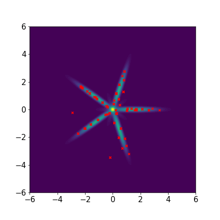
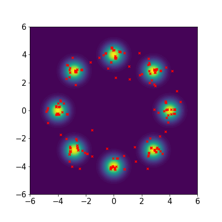
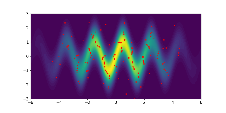
To illustrate this point, we construct a toy example to demonstrate different patterns of the decreasing curves with different bandwidth settings. For a given , we generate samples from the model , where is sampled from a two-dimensional standard Gaussian distribution and is sampled from the fully specified target distribution, an eight-component Gaussian mixture distribution (the second toy example in Section 4.1). It is obvious that as , converges to the target distribution. Indeed, in the right panel of Figure 1, the samples (red dots) are closer to the Gaussian mixture distribution (green contour plot) as . Using the Gaussian kernel, we compute for different and values. It is expected that all MMD2 curves decrease to zero as as shown in the left panel of Figure 1. But they have very different decreasing patterns. For , the decreases very fast initially when is small but much slower when is close to . For , the trend of is completely opposite. The curves are flat initially for in the range of and drop to zero very fast near the end.
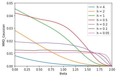
In this toy example, samples of different values mimic the particles that are evolving toward the target distribution in the EVI-MMD algorithm. Generalizing this observation to any MMD-based algorithm, the convergence of the particles is not at the optimal speed if is fixed throughout the algorithmic iteration. Therefore, we should choose a relatively large at the beginning of the iteration and gradually decrease . In this way, we can take advantage of the fast decent of MMD2 both at the early and end stages of the algorithm and avoid the plateau. The idea behind such an operation is “exploration v.s. exploitation”. In the early stage, with a large , the particles would explore a large neighborhood to find the region with a higher density of the target distribution. As the algorithm proceeds, when most particles are already at the region with a high probability density, the particles only need to exploit their close neighborhood and adjust their positions relative to other particles. As a result, the particles appear to align more regularly as shown in the toy examples in Section 4.1
Based on this idea, we propose to specify the bandwidth as follows,
| (18) |
where is the iteration index and , , and are three user-specified parameters. Among them, and we set it to be the median of the pairwise distance between the initial particles. In our examples, the initial distribution is a uniform distribution with a proper domain. The domain is obtained from the fully specified target distribution or from the training data in two-sample problems. The parameter is a regulatory parameter, which serves as a lower bound of . It is not very influential to the algorithm since it is only to stop from becoming zero. For lower-dimensional problems, such as the examples in Section 4.1 and 4.2, we set . For high-dimensional problems, such as the image data in Section 4.3, we set . In fact, in all our examples, when (in Algorithm 2), is still significantly larger than , and the largest maxIter we have used is 5000 (in this case is also very large). The parameter decides the rate of decrease of the bandwidth with respect to . More discussion about the tuning parameters is in Section 3.4
3.4 EVI-MMD with Adaptive Bandwidth
We summarize the EIV-MMD method using the Gaussian kernel and the adaptive bandwidth selection in Algorithm 2. For the problem with a fully specified target distribution, the free energy is
For the two-sample problem (training data size is ), the free energy is
The constant term (first term) in the free energy is not relevant to the optimization with respect to the particles and thus they are not computed in the optimization. For the large two-sample problems, the cross term and square term (the second and third term) are computed using the mini-batch procedure to save computation. There are many methods available to solve the proximal point minimization in each iteration. We have chosen the L-BFGS method (Liu and Nocedal, 1989) and it performs adequately.
-
: initial distribution of the particles. By default, we use the uniform distribution with a proper domain
-
: we set , the dimension of the problem
-
: total number of particles
-
: the size of samples to generate for or the size of the mini-batch
-
maxIter: the maximum number of iterations
-
, : parameters for vanishing bandwidth for the Gaussian kernel
In Appendix A1, we use the eight-component Gaussian mixture as the target distribution and show the performance of Algorithm 2. Different combination of , , and are used. From this example and many other simulation studies we have done, we recommend the following settings for all the tuning parameters.
-
•
-
•
is the median of all the pairwise distances between the initial particles.
-
•
is 0.01 or 1 depending on the dimension of the problem.
-
•
is mostly selected by trial-and-error and the usual candidates we have tried are .
-
•
is set based on the dimension of the problem as well as the constraint of the computation cost. In general, a bigger value leads to more accurate estimations of the free energy and its derivative.
-
•
maxIter should be large enough to ensure the convergence of MMD2 and the particles.
-
•
is largely based on consideration of the computational cost.
Although we recommend these rules-of-thumb on the tuning parameters, users should still run multiple trials to select the best possible combination of the tuning parameters for their problems in practice.
4 Numerical Examples
In this section, we demonstrate the performance of the proposed EVI-MMD algorithm through three types of examples. They cover two scenarios in which the target distribution is fully specified and the two-sample problems. In the latter case, the EVI-MMD is an effective generative model.
In all examples, we set as the median of the pairwise distance of the initial particles and . We set for the examples in Section 4.1 and 4.2 and in Section 4.3. For the parameter , through trial-and-error, we set for the examples in Section 4.1 and 4.3 and and in Section 4.2. All algorithms and examples are implemented in Pytorch 1.10.1 (Paszke et al., 2019). The computation was performed on the Open Science Grid (Pordes et al., 2007; Sfiligoi et al., 2009).
4.1 Toy Examples
We test the Algorithm 2 in three toy examples where the target distributions are listed below.
-
1.
Star-shaped five-component Gaussian mixture distribution:
where for ,
-
2.
Eight-component Gaussian mixture distribution:
where , , , , , , , , and .
-
3.
Wave-shaped distribution:
Although the first two distributions are both Gaussian mixture distributions, the eight-component Gaussian mixture distribution is more challenging since the effective support region for each Gaussian component is not connected, unlike the star-shaped distribution.
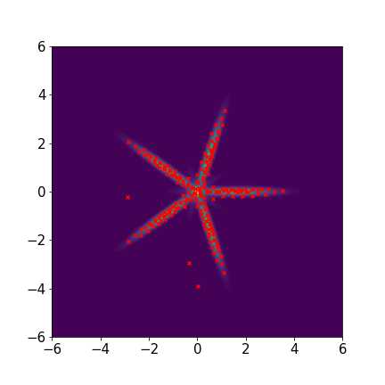
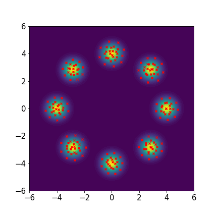
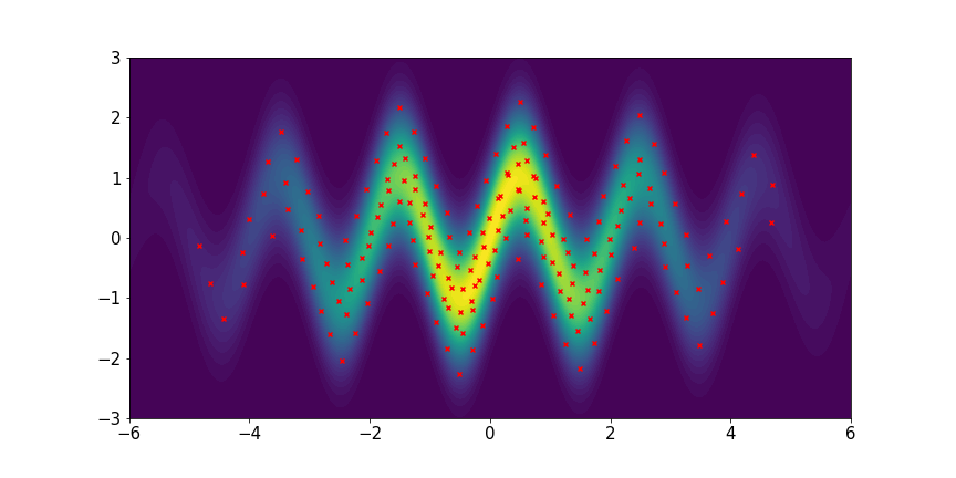
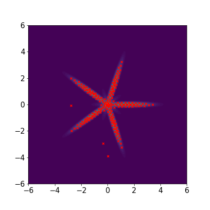
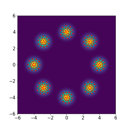
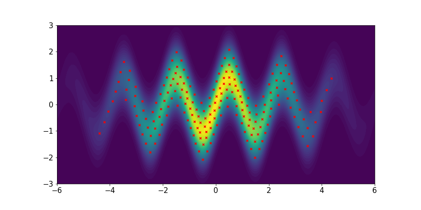
We set and maxIter=5000 for all three examples. The initial distributions are Uniform, Uniform, and Uniform, respectively. The three rows of sub-figures in Figure 2 show the particles at the 50th, 500th, and 5000th iteration. We see that most particles have been moved to the high-density region around the 500th iteration. At the 5000th iteration, all particles have been aligned quite regularly and the algorithm definitely reaches convergence.
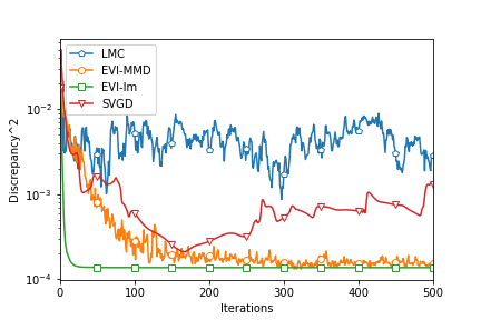
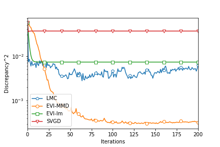
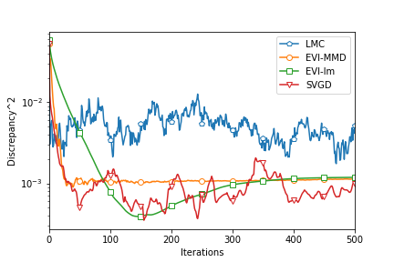
We compare the proposed Algorithm 2 with other similar methods, including the EVI-Im by Wang et al. (2021), SVGD by Liu (2017), and Langevin Monte Carlo (LMC) by Rossky et al. (1978). For the EVI-Im and SVGD methods, we set the step size and a fixed bandwidth for the Gaussian kernel. The tuning parameters of LMC are , , and , which decides the step size of LMC by the equation (different from the proposed algorithm).
To fairly compare the four algorithms, we compute the MMD2 criterion using a fixed bandwidth . So this MMD2 is not the objective function of any algorithms in this comparison. Figure 3 shows the decreasing MMD2 with respect to iterations of all the algorithms. Since both EVI-Im and EVI-MMD use the implicit Euler scheme, it is reasonable to compare the MMD2 in each iteration. The two methods have two embedded loops in Algorithm 1. The outer loop is indexed by and it is for each complete update of all particles. The inner loop is to minimize the objective function using L-BFGS. But SVGD and LMC only have a single loop. So we compare every 100 iterations of SVGD and LMC with 1 iteration (outer iteration indexed by ) of EVI-Im and EVI-MMD. This actually favors SVGD and LMC because the inner loop of EVI-Im and EVI-MMD is usually much less than 100 iterations. From Figure 3 we can see that the EVI-MMD has the fastest descent in the second and third examples and only second to EVI-Im in the first example. Both EVI-MMD and EVI-Im are more stable than SVGD and LMC.
4.2 Gaussian Distribution with Increasing Dimension
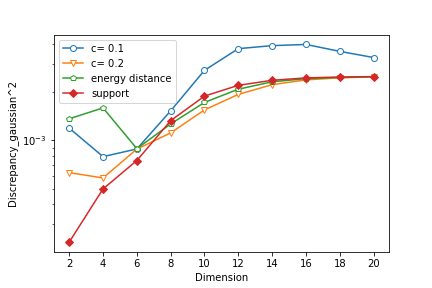
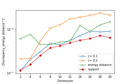
In this example, we study the performance of the proposed algorithm with respect to the increasing dimension. We compare the EVI-MMD with the adaptive bandwidth for the Gaussian kernel with two alternative methods:
- •
-
•
Support-Points: this method is proposed by Mak and Joseph (2018), which minimizes the same energy distance by a combination of the convex-concave procedure (CCP) with the resampling method.
The Energy-Distance method and the Support-Points method both minimize the same objective function but use different minimization methods. The EVI-MMD method and the Energy-Distance method minimize different objective functions but use the same implicit method.
We sample the training data of size from a standard Gaussian distribution with . For all three methods, we set the size of the particles and the initial distribution is Uniform. For EVI-MMD and Energy-Distance, we set and use the mini-batch size of . Only for EVI-MMD, we have tried and . For Support-Points, the default settings suggested by Mak and Joseph (2018) are used, except for the initial distribution. Figure 4 compares the MMD2 (Gaussian kernel with fixed ) and energy distance by (3) of the final particles returned by the three methods for . It is not surprising that both criteria become larger as the dimension increases whereas the sample size is fixed at 500, and the increasing trend is not linear but concave instead. Judging based on the MMD2 criterion, the EVI-MMD with has a similar performance with the two alternative methods. If using the energy distance criterion, the EVI-MMD with is comparable to the Support-Points method. Note that the y-axis is in log-scale, so the differences between these methods are not significant.
4.3 Generative Learning
Generative learning models have been widely used in various machine learning applications. They can solve supervised and unsupervised learning problems. Simply put, the generative learning model generates new samples based on the training data. More advanced generative learning models are combined with deep neural networks (Jabbar et al., 2021), Naive Bayes, Gaussian mixture model, hidden Markov model, etc. (Harshvardhan et al., 2020). In this example, we use the simplest nonparametric generative learning setup and apply the EVI-MMD to three benchmark image datasets, MNIST (LeCun et al., 1998), Fashion-MNIST (Xiao et al., 2017), and Cifar10 (Krizhevsky and Hinton, 2009).
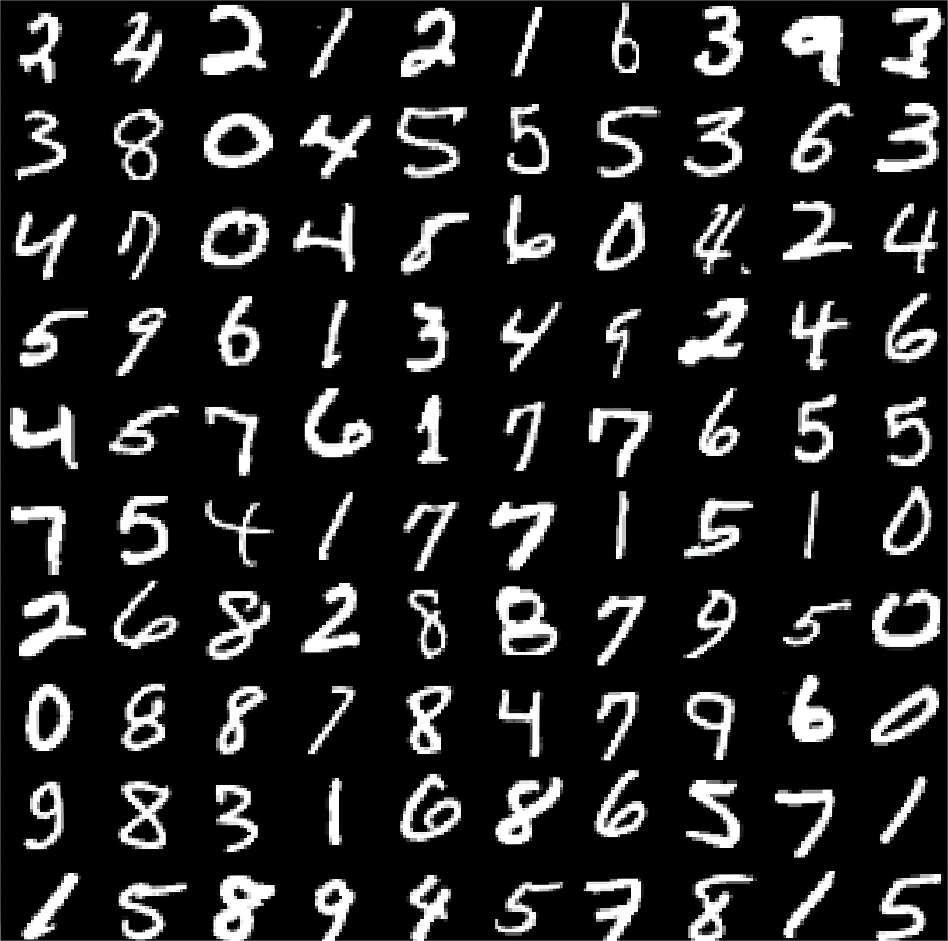
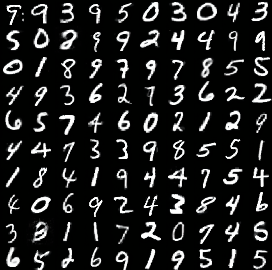
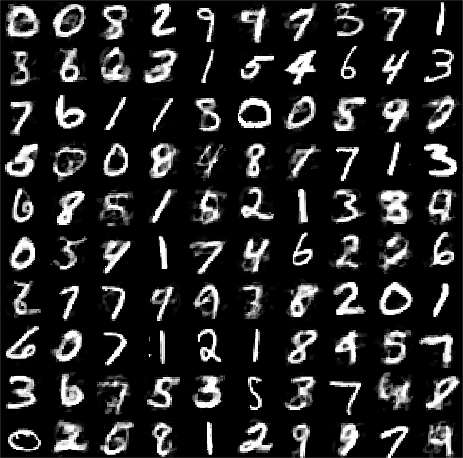

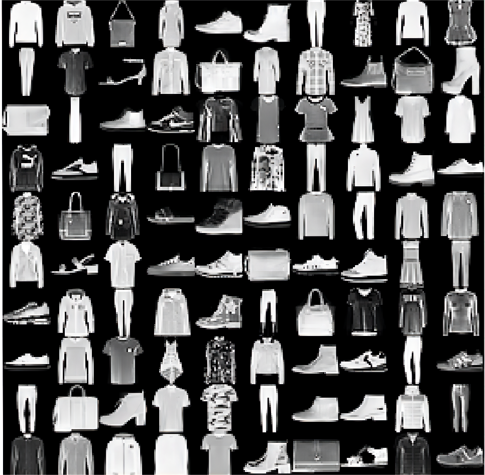
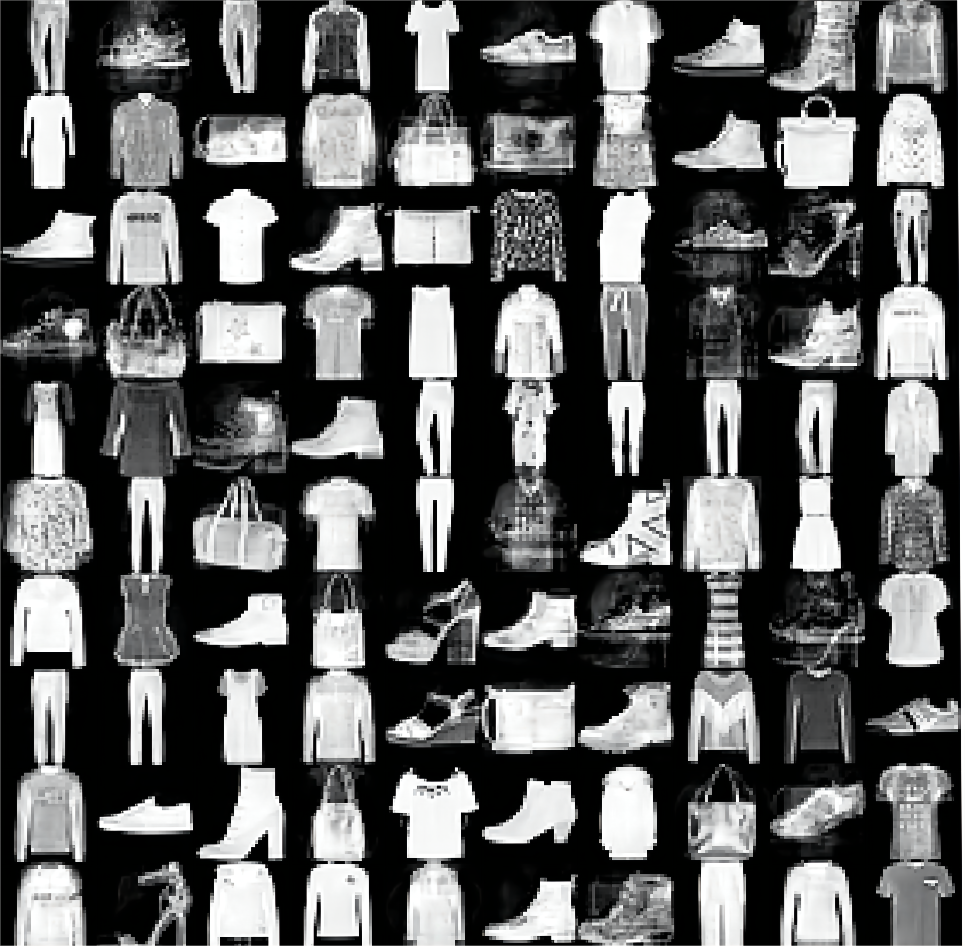
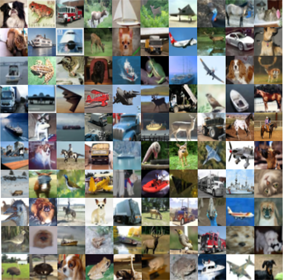
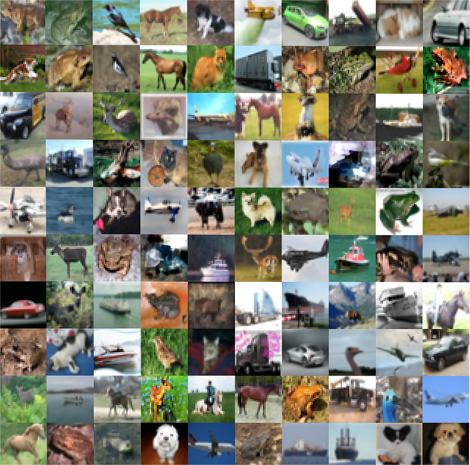
For the MNIST and Fashion-MNIST datasets, each data point is a grey image of size of pixels. For the Cifar10 dataset, each data point is a full-color image of size of pixels. One pixel value is in . All three are extremely high-dimensional two-sample problems. For the MNIST and Fashion-MNIST datasets, we use the whole dataset of size as the training data and resample a mini-batch of samples in each iteration. However, for the Cifar10 dataset, due to the extremely high dimension, we randomly choose a subset of images as the training data and also use the mini-batch of the size of . We choose , which is relatively small considering the dimension, is mainly due to the limited computing resources, but it has been proved to be sufficient.
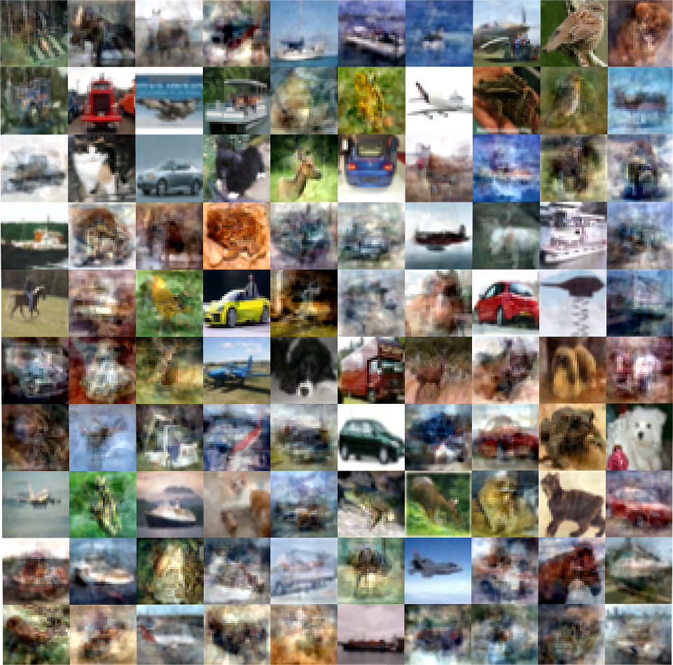
We generate new imagines using the EVI-MMD method and the Energy-Distance method defined in Section 4.2111We do not include the Support-Points method in this comparison because some issues with the R codes by Mak and Joseph (2018). We are not sure the reason but the returned results do not show any sign of convergence.. The initial particles are sampled from a uniform distribution in . We terminate both algorithms at for the EVI-MMD method. Figure 5 compares side-by-side 100 training data randomly chosen from the original training data (left column), new images generated by EVI-MMD (middle column), and Energy-Distance (right column). Both the training and new images are put into a panel. We can see the new images generated by both methods are very similar to the training data, and the EVI-MMD returns slightly sharper images than the Energy-Distance method.
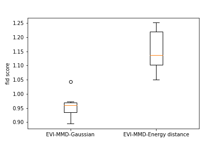
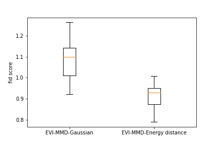
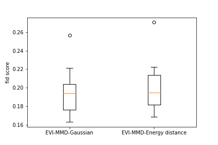
To provide a numerical comparison of the two methods, we calculate the FID score (Heusel et al., 2017) of the generated images. Due to the high computational cost, we randomly sample a subset of 500 images from the training data and calculate the FID score between the new images and the subset of training images. Repeating this 10 times we obtain 10 FID scores for each example. Figure 6 shows the boxplots of all the FID scores for the two methods for all three examples. We can see that both methods have a comparable FID score and the EVI-MMD outperforms the Energy-Distance in the MNIST and Cifar10 examples, which is consistent with the visual comparison in Figure 5.
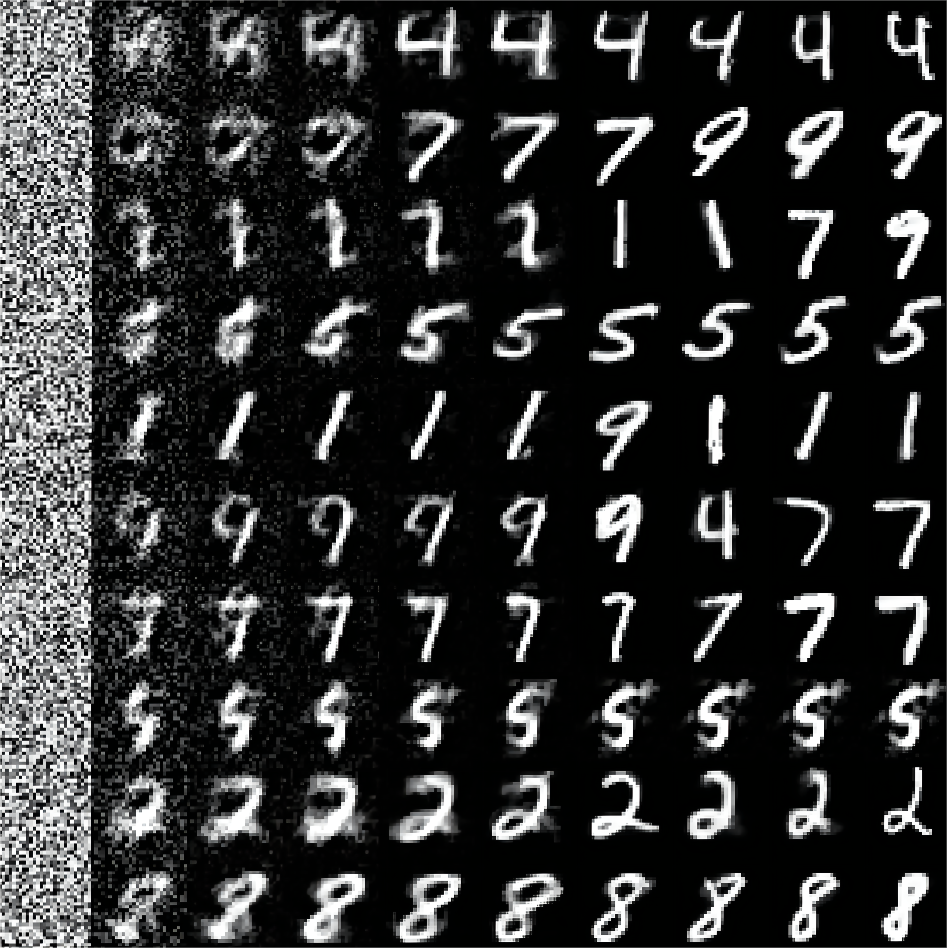
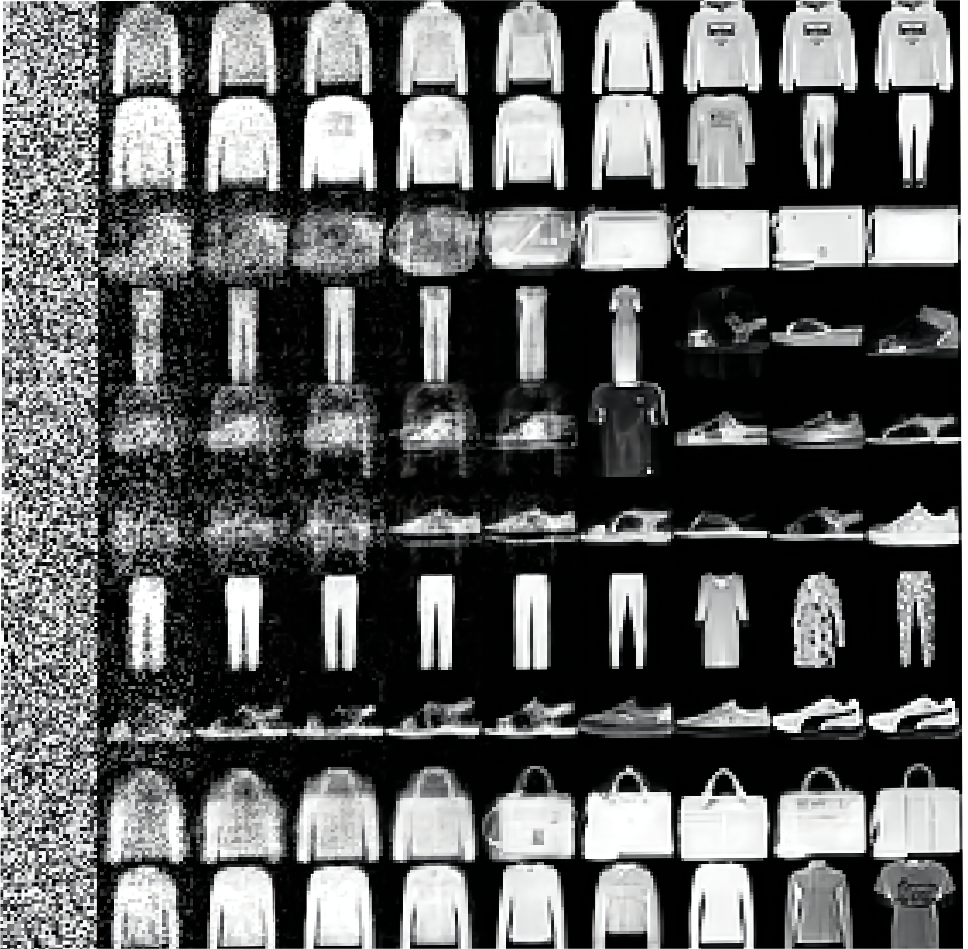
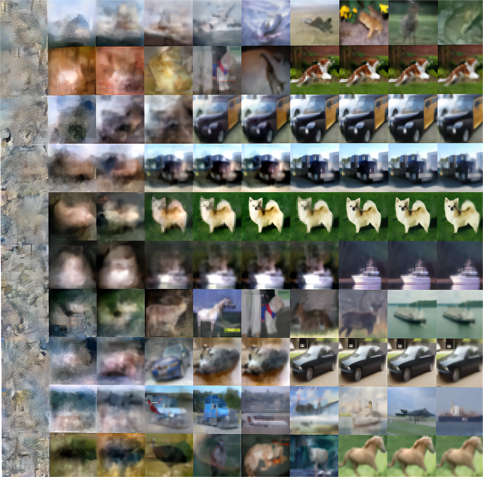
We also provide the trajectory of the EVI-MMD method in Figure 7. It shows the evolution of some randomly picked particles from static images to the final sharp images. Interestingly, some images are switched directions in the middle of their trajectories. For example, in the second row of the middle panel, the image suddenly switched from a top to a dress then to a pair of pants. This is because when we resample a mini-batch in each iteration. New images can appear in the mini-batch while some old images are not selected, causing the particles to constantly change to approximate the mini-batch data. Note that the EVI-MMD is by no means the best approach for the MNIST benchmark example. Readers can find many more sophisticated generative learning approaches that return better results. However, the EVI-MMD is probably the simplest by comparison and its results are adequate.
5 Conclusion
In this paper, we develop a new deterministic sampling method to approximate a target distribution by minimizing the kernel discrepancy, alternatively known as maximum mean discrepancy (MMD). The minimization of MMD is solved by the general energetic variational inference (EVI) framework first introduced by Wang et al. (2021). Specifically, we use the quadratic dissipation functional of the EVI and apply the particle approximation to the continuous energy-dissipation law, which is then followed by the variation procedure. This leads to a dynamic system that moves the particles from their initial positions to the target distribution. Using the implicit Euler scheme to solve this dynamic system, we obtain a special algorithm based on the EVI framework to minimize MMD, which we call EVI-MMD algorithm. In each iteration of updating the particles, we solve a proximal minimization problem using algorithms such as L-BFGS. To overcome the long-existing issue of bandwidth selection of the Gaussian kernel, we propose a novel way to specify the bandwidth dynamically. Other than approximating a fully specified distribution that is difficult to sample from, the EVI-MMD algorithm can also be used as a generative learning model for two-sample problems.
The EVI framework is very general. Many new variational inference methods can be proposed if we choose different combinations of the key ingredients, such as different divergence functions, order of variational and discretization via particles, parametric or non-parametric model for the flow map, and various numerical schemes for solving the dynamic system, etc. In fact, some existing methods can be also included in the EVI framework. The unified EVI framework also paves the way for a unified theoretical foundation for similar algorithms. We will keep pursuing these directions and fully explore the potentials of the EVI framework.
Acknowledgment
This research was done using services provided by the OSG Consortium (Pordes et al., 2007; Sfiligoi et al., 2009), which is supported by the National Science Foundation awards # 2030508 and # 1836650. We thank the editor, associate editor, and two reviewers for their valuable comments and suggestions. L. Kang’s work is partially supported by the National Science Foundation Grants DMS-1916467 and DMS-2153029. Y. Wang and C. Liu are partially supported by the National Science Foundation Grant DMS-1759536, DMS-1950868, and DMS-2153029.
A1 Appendix: One Example using Different Tuning Parameters
We study the effects of the tuning parameters on the proposed EVI-MMD approach in Algorithm 2. We use the same eight-component Gaussian mixture distribution in Section 4.1 for demonstration. In Section 4.1, the tuning parameters are: , the pairwise distance between the initial particles, , and . The algorithm has performed well under these settings.
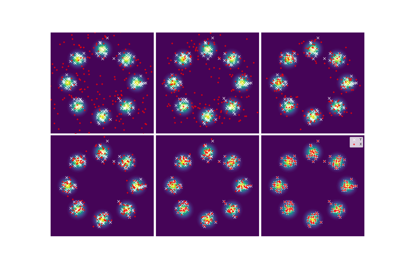
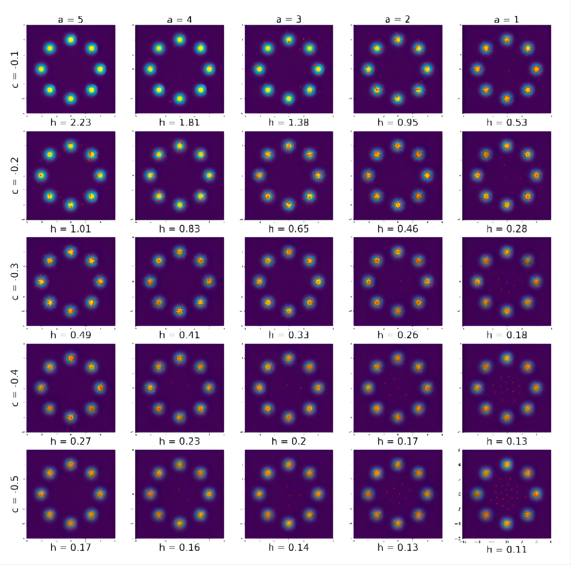
Figure A1 shows the particles returned by Algorithm 2 with iterations and different combinations of and . The other tuning parameters are set in the same way in Section 4.1. Under each sub-figure in Figure A1, the value is the returned by the proposed adaptive bandwidth in (18) when . From Figure A1, we can see that the best results are returned by and and 5, and the corresponding are 0.16 and 0.17. This confirms our recommendation that and should not be too small so that is large enough at the early stage of the procedure.
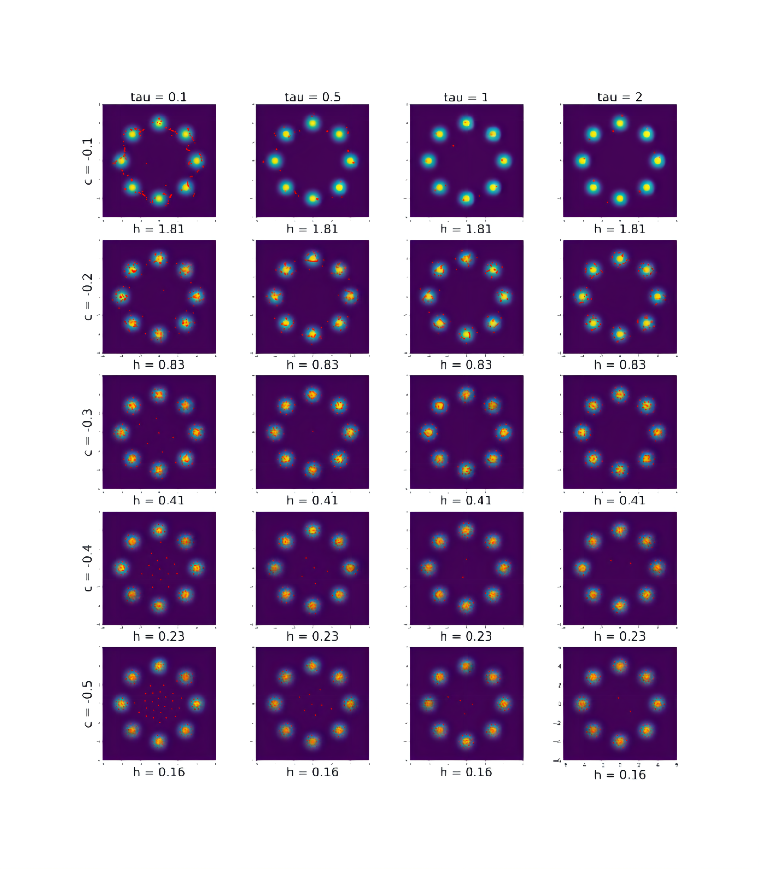
Figure A2 shows the particles returned by Algorithm 2 with iterations and different combinations of and . The other parameters remain the same settings as in Section 4.1. For example, . As the same as in Figure A1, the value for each sub-figure is returned by (18) when . For this example, still leads to the best results compared to other values and a larger is better than smaller ones. The best performance is brought by , which is the dimension of the problem. So it is consistent with our recommendation in Section 3.4.
References
- Bernton (2018) Bernton, E. (2018), “Langevin Monte Carlo and JKO splitting,” in Conference On Learning Theory, pp. 1777–1798.
- Bińkowski et al. (2018) Bińkowski, M., Sutherland, D. J., Arbel, M., and Gretton, A. (2018), “Demystifying mmd gans,” arXiv preprint arXiv:1801.01401.
- Blei et al. (2017) Blei, D. M., Kucukelbir, A., and McAuliffe, J. D. (2017), “Variational inference: A review for statisticians,” J. Am. Stat. Assoc., 112, 859–877.
- Briol et al. (2019) Briol, F.-X., Barp, A., Duncan, A. B., and Girolami, M. (2019), “Statistical inference for generative models with maximum mean discrepancy,” arXiv preprint arXiv:1906.05944.
- Chen et al. (2018a) Chen, C., Zhang, R., Wang, W., Li, B., and Chen, L. (2018a), “A unified particle-optimization framework for scalable bayesian sampling,” arXiv preprint arXiv:1805.11659.
- Chen et al. (2019) Chen, P., Wu, K., Chen, J., O’Leary-Roseberry, T., and Ghattas, O. (2019), “Projected Stein variational Newton: A fast and scalable Bayesian inference method in high dimensions,” in Advances in Neural Information Processing Systems, pp. 15130–15139.
- Chen et al. (2018b) Chen, W. Y., Mackey, L., Gorham, J., Briol, F.-X., and Oates, C. (2018b), “Stein Points,” in Proceedings of the 35th International Conference on Machine Learning, eds. Dy, J. and Krause, A., PMLR, vol. 80 of Proceedings of Machine Learning Research, pp. 844–853.
- Cheng and Boots (2017) Cheng, C.-A. and Boots, B. (2017), “Variational Inference for Gaussian Process Models with Linear Complexity,” in Advances in Neural Information Processing Systems 30, eds. Guyon, I., Luxburg, U. V., Bengio, S., Wallach, H., Fergus, R., Vishwanathan, S., and Garnett, R., Curran Associates, Inc., pp. 5184–5194.
- Cheng et al. (2018) Cheng, X., Chatterji, N. S., Bartlett, P. L., and Jordan, M. I. (2018), “Underdamped Langevin MCMC: A non-asymptotic analysis,” in Conference on learning theory, PMLR, pp. 300–323.
- Cheng and Xie (2021) Cheng, X. and Xie, Y. (2021), “Neural Tangent Kernel Maximum Mean Discrepancy,” arXiv preprint arXiv:2106.03227.
- Creswell et al. (2018) Creswell, A., White, T., Dumoulin, V., Arulkumaran, K., Sengupta, B., and Bharath, A. A. (2018), “Generative adversarial networks: An overview,” IEEE Signal Processing Magazine, 35, 53–65.
- Csiszár et al. (2004) Csiszár, I., Shields, P., et al. (2004), “Information Theory and Statistics: A Tutorial,” Foundations and Trends® in Communications and Information Theory, 1, 417–528.
- Damianou et al. (2016) Damianou, A. C., Titsias, M. K., and Lawrence, N. D. (2016), “Variational inference for latent variables and uncertain inputs in Gaussian processes,” The Journal of Machine Learning Research, 17, 1425–1486.
- E et al. (2020) E, W., Ma, C., and Wu, L. (2020), “Machine learning from a continuous viewpoint, I,” Science China Mathematics, 1–34.
- Fang et al. (2000) Fang, K.-T., Lin, D. K., Winker, P., and Zhang, Y. (2000), “Uniform design: theory and application,” Technometrics, 42, 237–248.
- Fang et al. (2002) Fang, K.-T., Ma, C.-X., and Winker, P. (2002), “Centered -discrepancy of random sampling and Latin hypercube design, and construction of uniform designs,” Mathematics of Computation, 71, 275–296.
- Fang and Mukerjee (2000) Fang, K.-T. and Mukerjee, R. (2000), “Miscellanea. A connection between uniformity and aberration in regular fractions of two-level factorials,” Biometrika, 87, 193–198.
- Fukumizu et al. (2007) Fukumizu, K., Gretton, A., Sun, X., and Schölkopf, B. (2007), “Kernel measures of conditional dependence.” in NIPS, vol. 20, pp. 489–496.
- Giga et al. (2017) Giga, M.-H., Kirshtein, A., and Liu, C. (2017), “Variational Modeling and Complex Fluids,” in Handbook of Mathematical Analysis in Mechanics of Viscous Fluids, eds. Giga, Y. and Novotny, A., Springer International Publishing, pp. 1–41.
- Goodfellow et al. (2014) Goodfellow, I., Pouget-Abadie, J., Mirza, M., Xu, B., Warde-Farley, D., Ozair, S., Courville, A., and Bengio, Y. (2014), “Generative adversarial nets,” Advances in neural information processing systems, 27.
- Gorbach et al. (2018) Gorbach, N. S., Bauer, S., and Buhmann, J. M. (2018), “Scalable variational inference for dynamical systems,” Advances in Neural Information Processing Systems 30, 7, 4807–4816.
- Graves (2011) Graves, A. (2011), “Practical Variational Inference for Neural Networks,” in Advances in Neural Information Processing Systems 24, eds. Shawe-Taylor, J., Zemel, R. S., Bartlett, P. L., Pereira, F., and Weinberger, K. Q., Curran Associates, Inc., pp. 2348–2356.
- Gretton et al. (2012) Gretton, A., Borgwardt, K. M., Rasch, M. J., Schölkopf, B., and Smola, A. (2012), “A kernel two-sample test,” The Journal of Machine Learning Research, 13, 723–773.
- Harshvardhan et al. (2020) Harshvardhan, G., Gourisaria, M. K., Pandey, M., and Rautaray, S. S. (2020), “A comprehensive survey and analysis of generative models in machine learning,” Computer Science Review, 38, 100285.
- Heng et al. (2021) Heng, J., Doucet, A., and Pokern, Y. (2021), “Gibbs flow for approximate transport with applications to Bayesian computation,” Journal of the Royal Statistical Society: Series B (Statistical Methodology), 83, 156–187.
- Heusel et al. (2017) Heusel, M., Ramsauer, H., Unterthiner, T., Nessler, B., Klambauer, G., and Hochreiter, S. (2017), “GANs Trained by a Two Time-Scale Update Rule Converge to a Nash Equilibrium,” CoRR, abs/1706.08500.
- Hickernell (1998) Hickernell, F. (1998), “A generalized discrepancy and quadrature error bound,” Mathematics of computation, 67, 299–322.
- Hickernell (1999) Hickernell, F. J. (1999), “Goodness-of-fit statistics, discrepancies and robust designs,” Statistics & probability letters, 44, 73–78.
- Hickernell (2016) — (2016), “The trio identity for Quasi-Monte Carlo error,” in International Conference on Monte Carlo and Quasi-Monte Carlo Methods in Scientific Computing, Springer, pp. 3–27.
- Hickernell and Liu (2002) Hickernell, F. J. and Liu, M.-Q. (2002), “Uniform designs limit aliasing,” Biometrika, 89, 893–904.
- Hofert et al. (2021) Hofert, M., Prasad, A., and Zhu, M. (2021), “Quasi-random sampling for multivariate distributions via generative neural networks,” Journal of Computational and Graphical Statistics, 1–24.
- Hu et al. (2018) Hu, Z., Yang, Z., Salakhutdinov, R., and Xing, E. P. (2018), “On Unifying Deep Generative Models,” in International Conference on Learning Representations.
- Jabbar et al. (2021) Jabbar, A., Li, X., and Omar, B. (2021), “A survey on generative adversarial networks: Variants, applications, and training,” ACM Computing Surveys (CSUR), 54, 1–49.
- Jordan et al. (1999) Jordan, M. I., Ghahramani, Z., Jaakkola, T. S., and Saul, L. K. (1999), “An introduction to variational methods for graphical models,” Machine learning, 37, 183–233.
- Jordan et al. (1998) Jordan, R., Kinderlehrer, D., and Otto, F. (1998), “The variational formulation of the Fokker–Planck equation,” SIAM journal on mathematical analysis, 29, 1–17.
- King and Lawrence (2006) King, N. J. and Lawrence, N. D. (2006), “Fast variational inference for Gaussian process models through KL-correction,” in European Conference on Machine Learning, Springer, pp. 270–281.
- Kingma et al. (2014) Kingma, D. P., Mohamed, S., Jimenez Rezende, D., and Welling, M. (2014), “Semi-supervised learning with deep generative models,” Advances in neural information processing systems, 27, 3581–3589.
- Kingma et al. (2016) Kingma, D. P., Salimans, T., Jozefowicz, R., Chen, X., Sutskever, I., and Welling, M. (2016), “Improved variational inference with inverse autoregressive flow,” in Advances in neural information processing systems, pp. 4743–4751.
- Kingma and Welling (2013) Kingma, D. P. and Welling, M. (2013), “Auto-encoding variational bayes,” arXiv preprint arXiv:1312.6114.
- Krizhevsky and Hinton (2009) Krizhevsky, A. and Hinton, G. (2009), “Learning multiple layers of features from tiny images,” Tech. Rep. 0, University of Toronto, Toronto, Ontario.
- LeCun et al. (1998) LeCun, Y., Bottou, L., Bengio, Y., and Haffner., P. (1998), “Gradient-based learning applied to document recognition.” proceedings of the IEEE, 86, 2278–2324.
- Li et al. (2017) Li, C.-L., Chang, W.-C., Cheng, Y., Yang, Y., and Póczos, B. (2017), “MMD GAN: towards deeper understanding of moment matching network,” in Proceedings of the 31st International Conference on Neural Information Processing Systems, pp. 2200–2210.
- Li et al. (2020) Li, Y., Kang, L., and Hickernell, F. J. (2020), “Is a Transformed Low Discrepancy Design Also Low Discrepancy?” in Contemporary Experimental Design, Multivariate Analysis and Data Mining, Springer, pp. 69–92.
- Li et al. (2015) Li, Y., Swersky, K., and Zemel, R. (2015), “Generative moment matching networks,” in International Conference on Machine Learning, PMLR, pp. 1718–1727.
- Liu and Zhu (2017) Liu, C. and Zhu, J. (2017), “Riemannian Stein variational gradient descent for Bayesian inference,” arXiv preprint arXiv:1711.11216.
- Liu et al. (2019) Liu, C., Zhuo, J., Cheng, P., Zhang, R., and Zhu, J. (2019), “Understanding and Accelerating Particle-Based Variational Inference,” in International Conference on Machine Learning, PMLR, pp. 4082–4092.
- Liu and Nocedal (1989) Liu, D. C. and Nocedal, J. (1989), “On the limited memory BFGS method for large scale optimization,” Mathematical programming, 45, 503–528.
- Liu (2017) Liu, Q. (2017), “Stein variational gradient descent as gradient flow,” in Advances in neural information processing systems, pp. 3115–3123.
- Liu et al. (2016) Liu, Q., Lee, J., and Jordan, M. (2016), “A Kernelized Stein Discrepancy for Goodness-of-fit Tests,” in Proceedings of The 33rd International Conference on Machine Learning, eds. Balcan, M. F. and Weinberger, K. Q., New York, New York, USA: PMLR, vol. 48 of Proceedings of Machine Learning Research, pp. 276–284.
- Liu and Wang (2016) Liu, Q. and Wang, D. (2016), “Stein variational gradient descent: A general purpose bayesian inference algorithm,” in Advances in neural information processing systems, pp. 2378–2386.
- Louizos and Welling (2017) Louizos, C. and Welling, M. (2017), “Multiplicative Normalizing Flows for Variational Bayesian Neural Networks,” in Proceedings of the 34th International Conference on Machine Learning - Volume 70, JMLR.org, ICML’17, p. 2218?2227.
- Ma et al. (2019) Ma, Y.-A., Chen, Y., Jin, C., Flammarion, N., and Jordan, M. I. (2019), “Sampling can be faster than optimization,” Proceedings of the National Academy of Sciences, 116, 20881–20885.
- Mak and Joseph (2018) Mak, S. and Joseph, V. R. (2018), “Support points,” The Annals of Statistics, 46, 2562–2592.
- Micchelli et al. (2006) Micchelli, C. A., Xu, Y., and Zhang, H. (2006), “Universal Kernels.” Journal of Machine Learning Research, 7.
- Mnih and Rezende (2016) Mnih, A. and Rezende, D. J. (2016), “Variational inference for monte carlo objectives,” arXiv preprint arXiv:1602.06725.
- Nguyen and Bonilla (2013) Nguyen, T. and Bonilla, E. (2013), “Efficient variational inference for Gaussian process regression networks,” in Artificial Intelligence and Statistics, pp. 472–480.
- Nguyen and Bonilla (2014) Nguyen, T. V. and Bonilla, E. V. (2014), “Automated Variational Inference for Gaussian Process Models,” in Advances in Neural Information Processing Systems 27, eds. Ghahramani, Z., Welling, M., Cortes, C., Lawrence, N. D., and Weinberger, K. Q., Curran Associates, Inc., pp. 1404–1412.
- Onsager (1931a) Onsager, L. (1931a), “Reciprocal relations in irreversible processes. I.” Phys. Rev., 37, 405.
- Onsager (1931b) — (1931b), “Reciprocal relations in irreversible processes. II.” Phys. Rev., 38, 2265.
- Paszke et al. (2019) Paszke, A., Gross, S., Massa, F., Lerer, A., Bradbury, J., Chanan, G., Killeen, T., Lin, Z., Gimelshein, N., Antiga, L., Desmaison, A., Kopf, A., Yang, E., DeVito, Z., Raison, M., Tejani, A., Chilamkurthy, S., Steiner, B., Fang, L., Bai, J., and Chintala, S. (2019), “PyTorch: An Imperative Style, High-Performance Deep Learning Library,” in Advances in Neural Information Processing Systems 32, eds. Wallach, H., Larochelle, H., Beygelzimer, A., d'Alché-Buc, F., Fox, E., and Garnett, R., Curran Associates, Inc., pp. 8024–8035.
- Pordes et al. (2007) Pordes, R., Petravick, D., Kramer, B., Olson, D., Livny, M., Roy, A., Avery, P., Blackburn, K., Wenaus, T., Würthwein, F., Foster, I., Gardner, R., Wilde, M., Blatecky, A., McGee, J., and Quick, R. (2007), “The open science grid,” in J. Phys. Conf. Ser., vol. 78 of 78, p. 012057.
- Rayleigh (1873) Rayleigh, L. (1873), “Some General Theorems Relating to Vibrations,” Proceedings of the London Mathematical Society, 4, 357–368.
- Rezende and Mohamed (2015) Rezende, D. J. and Mohamed, S. (2015), “Variational inference with normalizing flows,” arXiv preprint arXiv:1505.05770.
- Rockafellar (1976) Rockafellar, R. T. (1976), “Monotone operators and the proximal point algorithm,” SIAM journal on control and optimization, 14, 877–898.
- Rossky et al. (1978) Rossky, P. J., Doll, J. D., and Friedman, H. L. (1978), “Brownian dynamics as smart Monte Carlo simulation,” The Journal of Chemical Physics, 69, 4628–4633.
- Salman et al. (2018) Salman, H., Yadollahpour, P., Fletcher, T., and Batmanghelich, K. (2018), “Deep Diffeomorphic Normalizing Flows,” arXiv preprint arXiv:1810.03256.
- Sfiligoi et al. (2009) Sfiligoi, I., Bradley, D. C., Holzman, B., Mhashilkar, P., Padhi, S., and Wurthwein, F. (2009), “The pilot way to grid resources using glideinWMS,” in 2009 WRI World Congress on Computer Science and Information Engineering, vol. 2 of 2, pp. 428–432.
- Shetha et al. (2015) Shetha, R., Wangb, Y., Khardona, C. R., and EDU, T. (2015), “Sparse variational inference for generalized gaussian process models,” in ICML, pp. 1301–1311.
- Shridhar et al. (2019) Shridhar, K., Laumann, F., and Liwicki, M. (2019), “A comprehensive guide to bayesian convolutional neural network with variational inference,” arXiv preprint arXiv:1901.02731.
- Székely and Rizzo (2013) Székely, G. J. and Rizzo, M. L. (2013), “Energy statistics: A class of statistics based on distances,” Journal of statistical planning and inference, 143, 1249–1272.
- Trillos and Sanz-Alonso (2020) Trillos, N. G. and Sanz-Alonso, D. (2020), “The Bayesian Update: Variational Formulations and Gradient Flows,” Bayesian Analysis, 15, 29 – 56.
- Villani (2021) Villani, C. (2021), Topics in optimal transportation, vol. 58, American Mathematical Soc.
- Wang et al. (2021) Wang, Y., Chen, J., Liu, C., and Kang, L. (2021), “Particle-based energetic variational inference,” Statistics and Computing, 31, 1–17.
- Welling and Teh (2011) Welling, M. and Teh, Y. W. (2011), “Bayesian learning via stochastic gradient Langevin dynamics,” in Proceedings of the 28th international conference on machine learning (ICML-11), pp. 681–688.
- Wibisono et al. (2016) Wibisono, A., Wilson, A. C., and Jordan, M. I. (2016), “A variational perspective on accelerated methods in optimization,” Proceedings of the National Academy of Sciences, 113, E7351–E7358.
- Wu et al. (2019) Wu, A., Nowozin, S., Meeds, E., Turner, R., Hernández-Lobato, J., and Gaunt, A. (2019), “Deterministic variational inference for robust Bayesian neural networks,” in 7th International Conference on Learning Representations, ICLR 2019.
- Xiao et al. (2017) Xiao, H., Rasul, K., and Vollgraf, R. (2017), “Fashion-MNIST: a Novel Image Dataset for Benchmarking Machine Learning Algorithms,” .
- Zhang et al. (2019) Zhang, M., Bird, T., Habib, R., Xu, T., and Barber, D. (2019), “Variational f-divergence minimization,” arXiv preprint arXiv:1907.11891.