A distance exponent for Liouville quantum gravity
Abstract
Let and let be the random distribution on which describes a -Liouville quantum gravity (LQG) cone. Also let and let be a whole-plane space-filling SLEκ curve sampled independent from and parametrized by -quantum mass with respect to . We study a family of planar maps associated with called the LQG structure graphs (a.k.a. mated-CRT maps) which we conjecture converge in probability in the scaling limit with respect to the Gromov-Hausdorff topology to a random metric space associated with -LQG.
In particular, is the graph whose vertex set is , with two such vertices connected by an edge if and only if the corresponding curve segments and share a non-trivial boundary arc. Due to the peanosphere description of SLE-decorated LQG due to Duplantier, Miller, and Sheffield (2014), the graph can equivalently be expressed as an explicit functional of a correlated two-dimensional Brownian motion, so can be studied without any reference to SLE or LQG.
We prove non-trivial upper and lower bounds for the cardinality of a graph-distance ball of radius in which are consistent with the prediction of Watabiki (1993) for the Hausdorff dimension of LQG. Using subadditivity arguments, we also prove that there is an exponent for which the expected graph distance between generic points in the subgraph of corresponding to the segment is of order , and this distance is extremely unlikely to be larger than .
1 Introduction
1.1 Context: distances in -Liouville quantum gravity
Let and let be a simply connected domain. Heuristically speaking, a -Liouville quantum gravity (LQG) surface is the surface parametrized by whose Riemannian metric tensor is given by
| (1.1) |
where is some variant of the Gaussian free field [She07] on , is the Euclidean metric tensor, and is the so-called dimension of -LQG. LQG is a natural model of a continuum random surface. One reason for this is that LQG is the conjectured scaling limit of various random planar map models, the most natural discrete random surfaces. The case when corresponds to pure gravity, which is the scaling limit of uniform random planar maps. Other values of arise from random planar maps weighted by the partition function of some statistical mechanics model, e.g., the uniform spanning tree (), the Ising model (), or a bipolar orientation (). For many such models, it is expected that the scaling limit of the statistical mechanics model on the planar map is described by an -type curve [Sch00] or a family of such curves, independent from the LQG surface, for or .
Since is a distribution, or generalized function, and is not well-defined pointwise, the formula (1.1) does not make rigorous sense. However, one can rigorously construct the volume form associated with the metric (1.1), which should be a regularized version of , where is the Euclidean volume form. This was accomplished in [DS11], where it was shown that several different regularization procedures for converge to the same limiting measure , the -quantum area measure induced by . See also [RV14a] and the references therein for a more general theory of regularized random measures. The procedure used in [DS11] also allows one to define a length measure on certain curves in (including and independent SLEκ-type curves for ).
A major problem in the study of LQG is to make sense of (1.1) as a random metric (distance function). This has recently been accomplished in the special case when by Miller and Sheffield in the series of works [MS16f, MS15c, MS15a, MS15b, MS16b, MS16c], using a random growth process called quantum Loewner evolution. For certain special types of quantum surfaces defined in [DMS14], the resulting metric space is isometric to a certain Brownian surface, a random metric space which locally looks like the Brownian map [Le 13, Mie13] and which arises as the scaling limit of certain uniform random planar maps. For example, the quantum sphere is isometric to the Brownian map and the -quantum cone is isometric to the Brownian plane [CL14]. In the case when , the problem of constructing a LQG metric remains open.
Another major problem is to determine the Hausdorff dimension of the -LQG metric, assuming that it exists. In the case when it is known that this dimension is 4 [Le 07]. For general it is predicted by Watabiki [Wat93] that the dimension of -LQG is a.s. given by
| (1.2) |
There have been several works which support the Watabiki prediction. The authors of [AB14] perform numerical simulations using the discrete GFF which agree with the formula (1.2). In [MS16f, Section 3.3], the authors give an alternative non-rigorous derivation of (1.2) using so-called quantum Loewner evolution processes. The works [MRVZ16, AK16] prove upper and lower bounds for the Liouville heat kernel. If one assumes a certain relationship between two exponents (which the authors of the mentioned papers are not able to verify), these estimates suggest upper and lower bounds for the LQG dimension; this will be discussed further in Section 1.6. There is also a related quantity for LQG, called the spectral dimension, which is expected to be equal to 2 for all values of [ANR+98]. This prediction is confirmed in the context of the Liouville heat kernel in [RV14b, AK16] and for a class of random planar maps in [GM17b].
In contrast to the above results, the recent work [DG16b] proves estimates for several natural approximations of the -LQG metric (different from the approximations considered in this paper) for small values of which contradict the Watabiki prediction; c.f. Section 1.6.
If the dimension of LQG is , it is expected that the diameter (with respect to the graph distance) of a random planar map with edges which converges in the scaling limit to LQG is typically of order . Hence computing the dimension of LQG is expected to be equivalent to computing the tail exponent for the diameter of a random planar map in the LQG universality class.
The goal of this article is to present some small progress toward the above two problems. Miller and Sheffield’s approach in the case does not have a direct generalization to other values of , since it relies on special symmetries which are specific to . Instead, we will use a different approach based on the peanosphere construction of [DMS14], which applies for all and which we will now describe.
1.2 The LQG structure graph
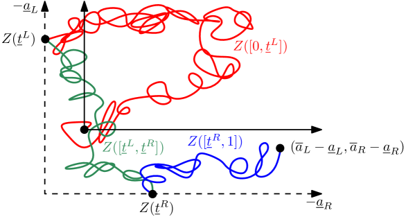
A peanosphere is a random pair consisting of a topological space and a space-filling curve on (with a specified parametrization) which is constructed from a correlated two-sided two-dimensional Brownian motion (see Figure 4). A peanosphere has a natural volume measure, which is defined by the condition that traces one unit of mass in one unit of time.
It is shown in [DMS14, Theorems 1.13 and 1.14] that there is a canonical (up to rotation) way to embed a peanosphere into in such a way that the following is true. The peanosphere volume measure is mapped to the -quantum area measure corresponding to a particular type of -LQG surface called a -quantum cone [DMS14, Definition 4.9]. Note that here is a variant of the GFF on . The curve is mapped to a space-filling variant111Our corresponds to the parameter in [MS17, DMS14]. of SLEκ, from to [MS17, Sections 1.2.3 and 4.3] which is sampled independently from and then parametrized in such a way that and the -quantum area is equal to for each . The correlation of the peanosphere Brownian motion is given by (for , this is proven in [GHMS17]). The two coordinates of this Brownian motion give the net change in the quantum lengths of the left and right sides of relative to time 0, respectively, so are denoted by and for . We write for the peanosphere Brownian motion. See Section 2.1.2 and the references therein for more background on the above objects.
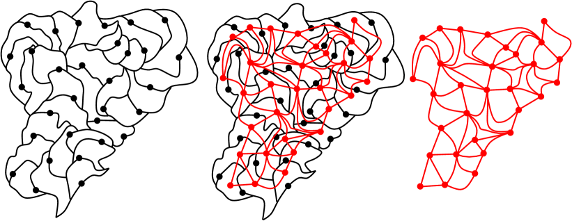
In this article, we will study a family of planar maps , called the LQG structure graphs(also called mated-CRT maps) associated with the pair , which we expect converges in the scaling limit in the Gromov-Hausdorff sense (when equipped with their graph distances) to an LQG metric induced by .
The vertices of the structure graph are the elements of . Two such vertices and are connected by an edge if the corresponding cells and intersect along a non-trivial boundary arc (i.e., a connected set with more than one point).222It is easy to see that is a planar map with the embedding given by mapping each vertex to the corresponding cell. In fact, is a triangulation provided we draw two edges instead of one between the cells and whenever and these cells intersect along a non-trivial arc of each of their left and right boundaries (equivalently, both conditions in (1.2) hold); see, the introduction of [GMS17b] for more details. In this paper we only care about graph distances in , so these facts will not be relevant for us. Note that this means that corresponds to the time interval for . See Figure 1 for an illustration of the above definition.
Remark 1.1.
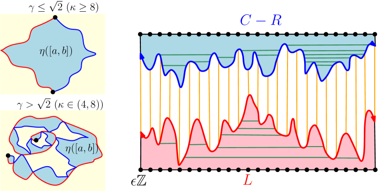
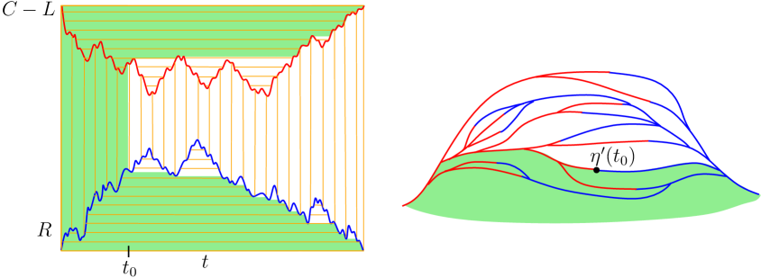
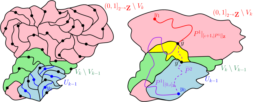
Figure 2, left, illustrates segments of space-filling SLE in the two phases and . If , then the cells for are each homeomorphic to the closed disk, and a.s. any two cells which intersect do so along a non-trivial connected boundary arc. If , however, the interiors of the cells are not connected since these cells can have “bottlenecks”. Moreover, a.s. there exist such that and intersect along a totally disconnected fractal set, but do not share a non-trivial connected boundary arc. In this case the and are not adjacent in .
The peanoshpere construction of [DMS14] implies that a.s. can equivalently be defined as the graph with vertex set , with with are connected by an edge if and only if either
| (1.3) |
See Figure 2, right, for an illustration of this adjacency condition. We note that Brownian scaling shows that the law of (as a graph) does not depend on , but it is convenient to view the family of graphs as being coupled together with the same Brownian motion.
The formula (1.2) tells us that is a discretization of the mating of the two continuum random trees constructed from the Brownian motions and (which is the reason for the term “mated-CRT map”). In particular, the LQG structure graphs can be defined using only Brownian motion, without any reference to LQG or SLE. In fact, all of the arguments of this paper except for the ones in Section 3 can be phrased entirely in terms of Brownian motion.
1.3 Structure graphs and distances in LQG
One of the main reasons for our interest in the graphs is the following conjecture.
Conjecture 1.2.
The appropriately normalized graph distances in the graphs converge in the scaling limit to a metric on -LQG. This metric is the scaling limit in the Gromov-Hausdorff topology of any random planar map model which converges to SLE-decorated -LQG in the peanosphere sense, including those studied in [She16b, KMSW15, GKMW18]. In the case when , the limiting metric coincides with the one in [MS15b, MS16b, MS16c] (which is itself isometric to the Brownian map [Le 14, Mie09]). Furthermore, the random walk on converges in the scaling limit to Liouville Brownian motion [Ber15, GRV16] on the limiting LQG surface.
The recent work [GMS17b] shows that random walk on converges to Brownian motion modulo time parametrization, which partially resolves the last part of Conjecture 1.2.
One a priori reason to expect that the LQG structure graphs should yield a metric on LQG in the scaling limit comes from comparison to discrete models. Indeed, many natural combinatorial random planar map models which belong to the -LQG universality class for some can be encoded by means of a two-dimensional random walk via a discrete analogue of the above encoding of the LQG structure graph in terms of a correlated two-dimensional Brownian motion. Planar maps for which this is the case include the uniform infinite planar triangulation (UIPT) [Ber07a, BHS18] () spanning tree-decorated planar maps [Mul67, Ber07b, She16b] (), bipolar-oriented planar maps [KMSW15] (), and Schnyder wood-decorated planar maps [LSW17] (). In the subsequent work [GHS17], we use this relationship to transfer the estimates proven here for LQG structure graphs to these discrete models (see also Section 1.6.3).
In [MS15b, Section 1.1], the structure graphs are suggested as a possible approach for constructing a metric on LQG. These graphs can also be viewed as a potential approach to [DMS14, Question 13.1]—which asks for a direct construction of a metric on the peanosphere—since they depend only on the Brownian motion .
In the present paper, we will prove non-trivial upper and lower bounds for the cardinality of a graph-distance ball of radius in (Theorem 1.10), which we expect should scale like , where is the dimension of -LQG. Hence our bounds can be interpreted as upper and lower bound for . As we will explain in Section 1.6 below, these bounds for are consistent with both the Watabiki prediction (1.2) and the estimates of [DG16b] and sharper than what can be obtained from [MRVZ16, AK16] (although there is presently no direct rigorous connection between our results and those of [MRVZ16, AK16, DG16b]).
We also prove that there is an exponent such that the expected graph distance between two typical vertices of the sub-graph of corresponding to the SLE segment is of order and the distance between two such vertices is extremely unlikely to be greater than (Theorems 1.12 and 1.15).
Although is special from the perspective of [MS15b, MS16b, MS16c], none of our results are specific to the case . We will, however, obtain stronger estimates than the ones in this paper for (which give, in particular, the correct exponent for the cardinality of a metric ball) in [GHS17] by comparing to a uniform random triangulation.
1.4 Basic notations
Here we record some basic notations which we will use throughout this paper.
Notation 1.3.
For and , we define the discrete intervals and .
Notation 1.4.
If and are two quantities, we write (resp. ) if there is a constant (independent of the parameters of interest) such that (resp. ). We write if and .
Notation 1.5.
If and are two quantities which depend on a parameter , we write (resp. ) if (resp. remains bounded) as (or as , depending on context). We write if for each (resp. ) as (resp. ). The regime we are considering will be clear from the context.
Unless otherwise stated, all implicit constants in , and and and errors involved in the proof of a result are required to depend only on the auxiliary parameters that the implicit constants in the statement of the result are allowed to depend on.
Remark 1.6.
For , we allow errors of the form to be infinite for large values of . In particular, the statement “” for some function means that for each , there exists such that for each we have .
We next introduce some notation concerning graphs.
Definition 1.7.
For a graph , we write for the set of vertices of and for the set of edges of .
Definition 1.8.
Let be a graph and let . A path of length in is a function for some such that either or is connected to by an edge in for each . We write for the length of .
Definition 1.9.
For a graph and vertices , we write for the graph distance from to in , i.e. the infimum of the lengths of paths in joining to . For a set , we write
We abbreviate . For and , the ball of radius centered at in is
For many of the statements in this paper, the choice of graph in Definition 1.9 will be important. Note that if is a subgraph of , then for each .
1.5 Main results
Throughout this subsection we assume we are in the setting of Section 1.2, so that is the family of LQG structure graphs constructed from an SLEκ-decorated -quantum cone for and . We make frequent use of Definition 1.9. Our first main result gives upper and lower bounds for the scaling dimension of .
Theorem 1.10.
Let and let
| (1.4) |
For each , there exists such that
where here is as the graph distance ball of radius (Definition 1.9).
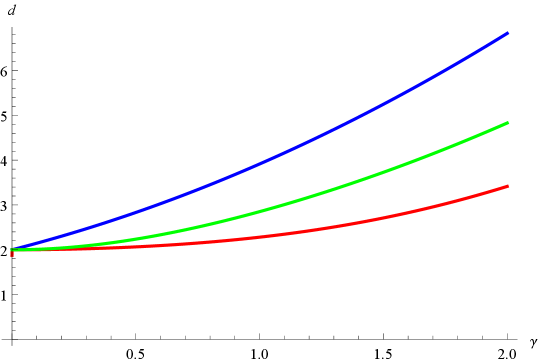
See Figure 3, left panel, for a graph of the bounds appearing in Theorem 1.10. By Brownian scaling, the laws of the graphs and for agree, so the statement of Theorem 1.10 is also true with in place of .
By Conjecture 1.2 we expect that the graph distance of (appropriately re-scaled) is a good approximation for the -LQG metric when is small. Hence it should be the case that in fact with high probability, where is the dimension of -LQG. Therefore Theorem 1.10 can be interpreted as giving upper and lower bounds for , namely . These bounds are consistent with the Watabiki prediction (1.2). In the special case when , we know that , so in this case we expect that with high probability when is large. This will be proven in [GHS17] by comparing to a uniform triangulation.
Our next main result is the existence of an exponent for distances in the LQG structure graphs. More precisely, we will consider distances in the sub-graphs of defined as follows.
Definition 1.11.
For a set , we write for the subgraph of whose vertex set is , with two vertices connected by an edge if and only if they are connected by an edge in .
Theorem 1.12.
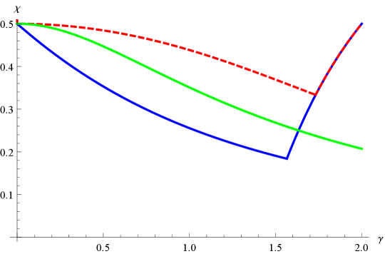
For , the limit
| (1.5) |
exists. Furthermore, we have
| (1.6) |
The exponent will be proven to exist via a sub-additivity argument. The reason for the quantity appearing in (1.6) is as follows. In the case when , the left and right outer boundaries of touch each other to form “bottlenecks” (c.f. Figure 2). These bottlenecks correspond to simultaneous running infima of and relative to time 0 (which a.s. do not exist for a non-positively correlated Brownian motion). The dimension of the time set for such that this is the case is [Eva85], so we expect that there are typically of order cells for which intersect a bottleneck. Any path from to 1 in must pass through each of these cells.
If we allow for paths between vertices of which traverse vertices in all of (rather than just in ) then bottlenecks do not pose a problem. Hence we still expect that (in the notation of Definition 1.9)
| (1.7) |
where is the dimension of -LQG; and that when there are either few or no bottlenecks. There are no bottlenecks for , and according to the Watabiki prediction (1.2), we have when . This leads to the following conjecture.
Conjecture 1.13.
Let be the dimension of -LQG. Then there exists such that for we have .
We do not have a prediction for the value of in Conjecture 1.13.
Remark 1.14.
We expect that it is possible to prove using the same estimates used to prove the lower bound in Theorem 1.10 plus some additional argument that in fact
| (1.8) |
where is as in (1.4). However, the argument needed to deduce (1.8) from the results in this paper requires some rather technical estimates for SLE and LQG and we do not find it to be particularly illuminating. Furthermore, we expect that if is as in Conjecture 1.13, then for the expected distance between generic points in along paths which are allowed to traverse any vertex of (not just vertices in ) is of order . Once this is known, (1.8) for becomes a trivial consequence of the estimates of this paper. We will say more about what is needed to prove (1.8) in Remark 3.9. See Figure 3, right panel, for a graph of our upper and lower bounds for .
Our next result estimates the probability that distances between vertices of are of order . We get an upper bound which holds except on an event of probability decaying faster than any power of and a lower bound which holds on an event of probability decaying slower than any power of .
Theorem 1.15.
Let and let be as in Theorem 1.12. There is a constant such that
| (1.9) |
Furthermore, for with , let (resp. ) be the element of closest to (resp. ). Then
| (1.10) |
Theorem 1.15 implies that for each ,
| (1.11) |
Note that Theorem 1.15 does not state that the diameter of is at least with uniformly positive probability. We expect, but do not prove, that this holds with probability tending to 1 as .
Remark 1.16.
The main difference between the estimates in this paper and the sorts of estimates which would be needed to obtain a non-trivial subsequential limit of the rescaled structure graphs in the Gromov-Hausdorff topology is the presence of “”-type errors. Indeed, if we could replace “” with “” and “” with “” in (1.9) we would have tightness due to the Gromov compactness criterion [BBI01, Theorem 7.4.15]. If we could also replace “” with “” and “” with “” in (1.10), then we would get that any subsequential limit is a non-trivial metric space with positive probability. We do not currently have a particular approach in mind for removing the errors in our estimates for general , but we expect that it is possible to get non-trivial subsequential scaling limits in our setting for small values of by adapting the arguments of [DD16].
1.6 Related works
1.6.1 Liouville heat kernel
The papers [MRVZ16, AK16] study the Liouville heat kernel, i.e. the heat kernel of the Liouville Brownian motion [Ber15, GRV16, GRV14]. As explained in [MRVZ16], if one assumes a certain relationship between two exponents which the authors are unable to verify, then the estimates of [MRVZ16] suggest that the dimension of -LQG should satisfy
| (1.12) |
In [AK16], a sharper upper bound is obtained which (subject to the same assumption about relationships between exponents) suggests that . Our upper and lower bounds from Theorem 1.10 are sharper (closer to the Watabiki prediction) than the upper and lower bounds of [MRVZ16, AK16] for all . There are currently no rigorous mathematical relationships between Theorem 1.10 and the results of [MRVZ16, AK16]. But, we conjecture that the random walk on converges to Liouville Brownian motion, which will link the two approaches.
1.6.2 Liouville first passage percolation
In addition to the structure graph, another natural approach to constructing a -LQG metric is to consider weighted graph distances on where each is assigned the weight , for a discrete GFF and a positive constant. This weighted graph distance is sometimes called Liouville first passage percolation (LFPP). It is natural to expect that LFPP converges in the scaling limit to the -LQG metric induced by a continuum GFF for (see, e.g., [DG16b, Footnote 1]).333The relation between and can be explained by observing that for a surface of dimension , rescaling areas by a constant should correspond to rescaling lengths by , and we can obtain such a rescaling by replacing by and , respectively. LFPP and its variants are studied in [DZ15, DG17, DD16, DG16a, DZ16, DG16b]. Here we highlight some aspects of this work which are most relevant to the topic of the present paper.
The paper [DD16] proves the existence of non-trivial subsequential scaling limits of LFPP (with respect to the Gromov-Hausdorff topology) for very small values of . In a sense, the results of [DD16] are orthogonal to the results of the present paper, since the present paper focuses on existence and bounds for scaling exponents and most of the results apply for all values of , but we do not prove existence of non-trivial subsequential limiting metrics; whereas [DD16] proves the existence of non-trivial subsequential limits for small values of but does not explicitly describe the scaling factors.
The work [DG16b] (c.f. [DG16a]) shows that the expected distance between typical points for the Liouville first passage percolation metric is at most a constant times with a universal constant for small enough ; and also proves similar upper bounds for related metrics defined using circle averages or balls of fixed -LQG mass for a continuum GFF. As pointed out in [DG16b], this estimate is inconsistent with the Watabiki prediction (1.2) since it suggests that for small enough whereas (1.2) implies that .
By contrast, our estimates are consistent with the Watabiki prediction for all . Even though the estimates of [DG16b] are not consistent with the Watabiki prediction, said estimates are consistent with the estimates of the present paper. In particular, our lower bound for (which we expect to be equal to at least for ) in Theorem 1.12 suggests that as , which does not contradict the upper bound .
At present, there is no rigorous mathematical relationship between LFPP but we expect that it may be possible to establish such a relationship. We plan to investigate this further in future work.
1.6.3 Other results for LQG structure graphs
The LQG structure graphs/mated-CRT maps are also studied in [DMS14, Section 10] (but not referred to as such), where they are used to prove that the peanosphere Brownian motion a.s. determines the pair .
In [GHS17], we use a strong coupling result for random walk and Brownian motion together with encodings of random planar maps in terms of random walk to prove that graph distances in the structure graph are comparable (up to polylogarithmic factors) to graph distances in a class of other natural random planar map models, including the uniform infinite planar triangulation and planar maps sampled with probability proportional to the number of spanning trees, bipolar-orientations, or Schnyder woods they admit. This allows us to transfer all of the results stated in Section 1.5 to these other random planar maps.
The paper [GMS17b] shows that random walk on converges to Brownian motion modulo time parametrization, which implies that the so-called Tutte embedding of (which, unlike the a priori embedding is an explicit functional of the graph) is asymptotically the same as the a priori embedding. The papers [GM17b, GH18] prove quantitative bounds for the simple random walk on and (via strong coupling) the aforementioned other random planar map models.
1.7 Outline
Here we give a moderately detailed overview of the remainder of the paper. In Section 2, we will review the definitions of LQG, space-filling SLE, and the peanosphere construction; and prove some basic facts about the structure graphs and about correlated two-dimensional Brownian motion.
In Section 3, we will use estimates for SLE-decorated LQG to prove quantitative estimates for distances in the -LQG structure graph, which will eventually lead to a proof of Theorem 1.10. These estimates are the only arguments in this paper which require non-trivial facts about LQG and SLE. In particular, to prove the upper bound in Theorem 1.10, we will prove bounds for the Euclidean diameter of structure graph cells and thereby a lower bound for the minimal number of cells in a path in from 0 to the boundary of . The lower bound in Theorem 1.10 will be deduced from a KPZ-type formula (Proposition 3.5) which gives us an upper bound for the number of cells needed to cover a line segment.
In Sections 4 and 5, we will prove the existence of the limit in (1.5) for restricted to powers of 2 using a subadditivity argument. We will also show that the diameter of is very unlikely to be larger than (Proposition 5.2). The key idea of the proof is that if we set then is approximately sub-multiplicative in the sense for a certain range of values of . This gives the existence of due to a variant of Fekete’s subaddivity lemma (Lemma 5.3).
Roughly speaking, to prove the sub-multiplicativity relation for we start with a path in of length and divide each of the cells hit by into sub-cells. Concatenating paths within each of these sub-divided cells gives us a path in whose length is at most the sum of terms with the same law as . The estimates of Section 4 are needed to allow us to compare the conditional law of the sub-divided cells given to their unconditional law.
Appendix A contains the proofs of some technical lemmas.
Acknowledgements We thank Jian Ding, Subhajit Goswami, Jason Miller, and Scott Sheffield for helpful discussions. E.G. was supported by the U.S. Department of Defense via an NDSEG fellowship. N.H. was supported by a doctoral research fellowship from the Norwegian Research Council. X.S. was supported by the Simons Foundation as a Junior Fellow at Simons Society of Fellows. We thank two anonymous referees for helpful comments on an earlier version of this article.
2 Preliminaries
2.1 Backgound on LQG and SLE
In this subsection we give a brief review of some basic properties of Liouville quantum gravity, space-filling SLE, and the peanosphere construction. Although these objects are the main motivation of this work, their non-trivial properties will only be used explicitly in Section 3. The proofs in the other sections can be phrased in terms of Brownian motion by means of the peanosphere construction. We refer to the cited references for further background.
2.1.1 Liouville quantum gravity
Fix . A -Liouville quantum gravity (LQG) surface, as defined in [DS11, She16a, DMS14, MS15c] is an equivalence class of pairs where is a simply connected domain and is a distribution on (typically some variant of the Gaussian free field on [She07, SS13, She16a, MS16d, MS17]). Two such pairs and are declared to be equivalent if there is a conformal map such that
| (2.1) |
As shown in [DS11], an LQG surface comes equipped with a natural volume measure , which is a limit of regularized versions of and is invariant under coordinate changes of the form (2.1). That is, if and are related as in (2.1) then a.s. for each Borel set [DS11, Proposition 2.1]. Similarly, an LQG surface has a natural length measure which is defined on certain curves in [DS11, Section 6], including and SLEκ-type curves for [DS11]. For , one can define quantum surfaces with marked points for by requiring that the map in (2.1) preserves the marked points.
In this paper we will mostly be interested in a particular type of LQG surface called an -quantum cone for (in fact we will almost always take ). This is an infinite-volume doubly-marked quantum surface introduced in [DMS14, Section 4.3]. The distribution is obtained from , where is a whole-plane GFF, by “zooming in” near the origin.
The distribution is called the embedding of the quantum surface into and is not uniquely determined by the equivalence class of . Indeed, by (2.1) one obtains another embedding into by replacing with for . There is a natural choice of embedding for a quantum cone called a circle average embedding, which is the embedding used in [DMS14, Definition 4.9] and is defined as follows. For , let be the circle average of over (as defined in [DS11, Section 3.1]). Then a circle average embedding is one for which and agrees in law with , where is a whole-plane GFF with additive constant chosen so that its circle average over is 0. We note that if is an arbitrary embedding into of an -quantum cone then there exists a random such that is a circle average embedding of . The modulus is a deterministic function of but is not.
2.1.2 Space-filling SLE
For , a whole-plane space-filling SLEκ from to is a variant of SLEκ which fills all of , even in the case when (so that ordinary SLEκ does not fill space). This variant of SLE is defined in [DMS14, Footnote 9], using chordal versions of space-filling SLE constructed in [MS17, Sections 1.2.3 and 4.3]. We will not need many specific facts about space-filling SLE in this paper, since we will primarily study the structure graphs from the Brownian motion (i.e., peanosphere) perspective. So, we only give a brief description of this object here and refer the reader to the above cited papers for more details.
In the case when , whole-plane space-filling SLEκ is just a two-sided version of chordal SLEκ. In the case when , whole-plane space-filling SLEκ is obtained by iteratively filling in the “bubbles” disconnected from by a two-sided variant of chordal SLEκ with SLEκ-type curves. If and is the (a.s. unique) time that hits , then the interface between and is the union of two coupled whole-plane SLE curves from to ([MS17, Theorem 1.1] and [DMS14, Footnote 9]) which intersect each other at points different from if and only if . These curves comprise the left and right outer boundaries of .
2.1.3 Peanosphere construction
Let and let . Let be a -quantum cone and let be a whole-plane space-filling SLEκ independent from . Suppose we parametrize by -quantum area with respect to , so that and for each with . For , let (resp. ) be the net change in the quantum length (with respect to ) of the left (resp. right) outer boundary of relative to time 0. In other words, is the quantum length of the set of points in the left outer boundary of which do not belong to the left outer boundary of minus the quantum length of the set of points in the left outer boundary of which do not belong to the left outer boundary of , and similarly for . Then by [DMS14, Theorem 1.13] there is a deterministic constant depending only on such that evolves as a correlated two-sided two-dimensional Brownian motion with
| (2.2) |
It is shown in[DMS14, Theorem 1.14] that a.s. determines , modulo rotation, but not in an explicit way. However, one can explicitly describe many functionals of in terms of . For example, hits the left (resp. right) outer boundary of and subsequently covers up a boundary arc of non-zero quantum length at time if and only if is a running infimum for (resp. ) relative to time 0. Furthermore, if then the left and right outer boundaries of intersect at if and only if is a simultaneous running infimum for and relative to time 0. Such simultaneous running infima occur if and only if is positively correlated [Shi85] which corresponds precisely to the case when .
Figure 4 describes how to construct a topological space decorated by a space-filling curve from . This object can be thought of as the structure graph with .
Definition 2.1.
A peanosphere is a random pair consisting of a topological space and a parametrized space-filling curve on , constructed from a correlated two-dimensional Brownian motion in the manner described in Figure 4.
It follows from the above discussion that a -quantum cone decorated by a whole-plane space-filling SLEκ is a canonical embedding of an infinite-volume peanosphere into .
2.2 Basic properties of the structure graph
Throughout this subsection, we fix and use the notation of Section 1.2, so in particular is a -quantum cone, is a whole-plane space-filling SLEκ for independent from and parametrized by -length, is the correlated Brownian motion from [DMS14, Theorem 1.13], and are the associated -structure graphs, with vertex set .
2.2.1 Boundary lengths
For with , the cell has four natural marked boundary arcs, corresponding to the set of points in which lie on either the left or right outer boundary of either or . We call these boundary arcs the lower left, lower right, upper left, and upper right boundary arcs. In terms of the peanosphere Brownian motion , the lower left (resp. right) boundary arc of is the image under of the set of such that (resp. ) attains a running infimum at time when running forward from time . Similarly, the upper left (resp. right) boundary arc of is the image of the set of such that (resp. ) attains a running infimum at time when running backward from time .
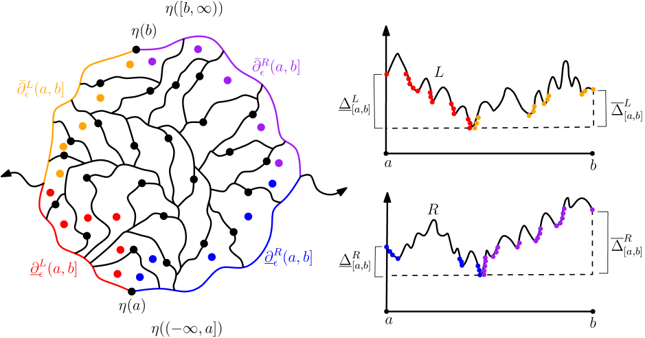
We will have occasion to consider four marked subsets of the vertex set of which correspond to the four marked boundary arcs of discussed above. We emphasize that these four subsets are not necessarily disjoint. See Figure 5 for an illustration.
Definition 2.2.
For and an (open, closed, or half-open) interval , we define the lower left boundary of to be the set of such that the following is true. There is a with such that the left boundaries of and share a non-trivial arc. We define the lower right boundary in the same manner with “right” in place of “left”. We define the upper left and upper right boundaries and similarly but with “” in place of “”. We define
so that is the set of all such that is adjacent to some element of in .
By (1.2), if then (resp. ) if and only if the Brownian motion (resp. its time reversal) attains a running infimum relative to the left (resp. right) endpoint of at time . The same holds with “” in place of “”.
The following is a convenient way of encoding the LQG lengths of the four marked boundary arcs of .
Definition 2.3.
For an interval and a path , we define the initial displacement and the final displacement of over by
For the peanosphere Brownian motion , we define the boundary length vector of over by
The reason for the notation , etc., in Definition 2.3 is that these quantities give the quantum lengths of the four marked boundary arcs of the cell introduced above (this is immediate from the definition of ; see Section 2.1.3). The main reason for our interest in the objects of Definition 2.3 is the following lemma.
Lemma 2.4.
Let be an interval (possibly infinite or all of ) and . The graph is measurable with respect to the -algebra generated by the boundary length vectors (in the notation of Definition 2.3)
| (2.3) |
Proof.
Let be the -algebra generated by the set (2.3). We first observe that for each with , we have
Consequently, . Similarly, , , and are all -measurable. On the other hand, the condition (1.2) for is equivalent to the condition that either
| (2.4) |
or the same holds with in place of . Thus the event that and are adjacent in is -measurable, and we conclude. ∎
2.2.2 Comparison of distances
In this subsection we record some elementary observations which allow us to compare distances in the graphs for different values of and .
Lemma 2.5.
Suppose , , , and . Then
| (2.5) |
In particular, stochastically dominates and for any with , stochastically dominates .
Proof.
Suppose is a path in with and . For , let be defined so that . By the definition of , and are either equal or share a non-trivial boundary arc for each , so also and are either equal or share a non-trivial boundary arc for each such . It follows that is a path in of length at most from to , which gives the left inequality in (2.5).
For the right inequality, suppose is a path in with and . Let and let be chosen so that shares a non-trivial boundary arc with . For , inductively let be chosen so that shares a non-trivial boundary arc with and let be chosen so that shares a non-trivial boundary arc with (unless , in which case we take ). Then is a path in from to with length , and we obtain the right inequality in (2.5). ∎
Lemma 2.5 allows us to compare the expected diameters of graphs of the form whenever the number of vertices is a non-negative integer power of 2. Our next lemma allows us to extend a weaker form of this comparison to the case when is not a power of 2.
Lemma 2.6.
Suppose and . Let and write where with . Then we have the following two estimates:
| (2.6) | ||||
| (2.7) |
Proof.
By scaling we can assume without loss of generality that . With as in the statement of the lemma, we can write , where are disjoint and each is the intersection of with some interval and satisfies . By translation and scale invariance,
This proves the first inequality in (2.6). The second inequality follows from the stochastic domination statement for diameters in Lemma 2.5. The estimate (2.7) is proven similarly. ∎
2.3 Brownian motion estimates
In this subsection we record some miscellaneous elementary estimates for Brownian motion which we will need several times in the remainder of this article. Throughout, we fix and we let be a correlated two-dimensional Brownian motion with variances and covariance , with as in (2.2). We start with a basic continuity estimate.
Lemma 2.7.
There are constants , depending only on , such that the following is true. Let
Then .
Proof.
This is a straightforward consequence of the Gaussian tail bound, the reflection principle, and a union bound over all dyadic intervals of the form for and . ∎
Next, we extract an estimate from [Shi85] for the probability of an “approximate -cone time” for . In the next lemma, for a set , we let be the set of points with Euclidean distance to .
Lemma 2.8.
Let and and set and . Then
| (2.8) |
with implicit constant depending only on . Furthermore, suppose that is the image of a smooth path starting from 0 and ending at , and let . Then
| (2.9) |
with the implicit constant depending on , , , and but not or .
Proof.
The estimate (2.8) follows from [Shi85, Equation (4.3)] (applied with ) after applying a linear transformation to to get an uncorrelated Brownian motion (c.f. the proof of [GMS17a, Lemma 2.2]). The estimate (2.9) follows from [Shi85, Theorem 2] together with the analogous statements for unconditioned Brownian motion and for Brownian motion conditioned to stay in a cone. ∎
We also have an estimate for the cardinality of the boundary of the graph , as defined in Definition 2.2, which is really just an estimate for Brownian motion.
Lemma 2.9.
For and , we have (in the notation of Definition 2.2) with implicit constant depending only on .
Proof.
By symmetry, it suffices to show that . If , then if and only if
| (2.10) |
The random variables on the left and right sides of (2.10) are independent. By the reflection principle, the random variable on the right has the law of times the modulus of a centered Gaussian random variable with variance . For each ,
By combining these observations, we find that for all . Clearly, . We conclude by summing over all . ∎
3 Quantitative distance bounds
In this section we will use space-filling SLE and LQG to prove estimates which will eventually lead to the bounds in Theorem 1.10 as well as the lower bound for in Theorem 1.12. This is the only section of the paper in which we directly use non-trivial facts about SLE and LQG; the rest of our arguments can be formulated solely in terms of Brownian motion. Some of the more standard LQG estimates used in this section are proven in Appendix A.
3.1 Upper bound for the cardinality of a ball
In this subsection we will prove the following lower bounds for distances in the LQG structure graph, which will eventually lead to the upper bound in Theorem 1.10 and the lower bound for in Theorem 1.12.
Proposition 3.1.
Corollary 3.2.
For each , there exists such that for each ,
| (3.4) |
Proof.
To prove Proposition 3.1, we will first use basic estimates for LQG to prove an upper bound for the number of space-filling SLE cells for with at least a given Euclidean diameter which are contained in a fixed Euclidean ball (Lemma 3.3). By considering the largest cells contained in , this estimate will lead to a lower bound for the minimal number of cells in a path in from 0 to a cell which lies outside of . Since a.s. contains a Euclidean ball centered at the origin (and one can estimate the radius of this ball) this will allow us to conclude Proposition 3.1. The in (3.2) and (3.3) comes from the fact that there are typically at least cells of which intersect the pinch points of (recall Figure 2, right panel).
We note that the only properties of space-filling SLEκ used in the proof is [GHM15, Proposition 3.4]—which says that a segment of space-filling SLEκ typically contains a Euclidean ball whose diameter is comparable (up to an exponent) to the diameter of the segment—and [HS16, Proposition 6.2] (which is used in Lemma A.4 to get a polynomial bound for the probability in (3.1)). Since these properties are true for every , Proposition 3.1 remains true, with the same exponents, e.g., if we replace by a space-filling SLE for , still sampled independently from and then parametrized by -LQG mass.
We now commence with the proof of Proposition 3.1. We first prove our estimate for the number of structure graph cells having a given Euclidean diameter.
Lemma 3.3.
Let be the circle average embedding of a -quantum cone in . Let be a space-filling from to in sampled independently from and then parametrized by -quantum mass with respect to . For , let
| (3.5) |
For each , there exists such that for each , it holds with probability at least that the number of such that and is at most
Proof.
The idea of the proof is to first argue that each cell of which intersects must contain a Euclidean ball of radius slightly smaller than the diameter of the cell; then use Lemma A.1 with in place of to upper bound the number of such Euclidean balls with radius at least .
Step 1: comparing space-filling SLE cells to Euclidean balls. Fix , to be chosen later. Also fix . For , let be the radius of the largest Euclidean ball contained in . Also let be the center of this ball. We claim that with probability at least ,
| (3.6) |
To see this, let be the event that for each and each with , , and , the set contains a Euclidean ball of radius at least . By [GHM15, Proposition 3.4 and Remark 3.9], we have . By considering separately the values of for which and , we find that for small enough (depending only on ), the relation (3.6) holds whenever occurs.
Step 2: bounding the number of Euclidean balls with -mass at most . For let be the set of with . By Lemma A.1 (applied with in place of and with ) and a sum over cells in the case when ; or the trivial bound in the case when , we have .
Since is non-decreasing, piecewise continuously differentiable, and satisfies for , there exists such that for . By the Chebyshev inequality and since is a non-negative integer (so equals 0 whenever it is ), we find that with probability at least ,
| (3.7) |
Step 3: conclusion. Now suppose that (3.6) holds and (3.7) holds with in place of , which happens with probability at least . If with and , then by (3.6) and since , we have . Since by definition, there is a with . By (3.7), the number of such is 0 if and is at most if , with the rate of the independent of . We now conclude by choosing sufficiently small (depending on ); and setting for this choice of . ∎
Proof of Proposition 3.1.
Fix to be chosen later, in a manner depending only on and . Also fix . We will apply Lemma 3.3 to bound the number of cells of contained in with -mass in a given interval, deduce from this a lower bound for the minimum length of a path in from 0 to a vertex whose corresponding cell lies outside of , then use this and a basic estimate for space-filling SLE to obtain (3.1). The other estimates in the proposition statement will follow from (3.1) and a lower bound for the Hausdorff dimension of the times for corresponding to pinch points of .
Step 1: application of Lemma 3.3. Let
be a partition of with for each . For , let be the set of with and . Also let be the set of with and . By Lemma 3.3 applied with in place of for each , it holds except on an event of probability decaying faster than some positive power of (the power depends on and ) that
| (3.8) |
where here is as in (3.5) and the error is independent of .
Step 2: bounding the -distance from 0 to . The condition (3.8) implies that the total Euclidean diameter of the cells corresponding to elements of satisfies
| (3.9) |
For as in the proposition statement, we have for . Consequently, if we choose sufficiently small (depending only on and ) then the right side of the inequality in (3.9) is smaller than for sufficiently small provided .
If (3.9) holds and is a path in from 0 to some with , then we can find distinct each of which is hit by and satisfies such that
Therefore, . Hence, except on an event of probability decaying faster than some positive power of ,
| (3.10) |
Step 3: bounding the -distance from 0 to . To transfer from (3.9) to a bound for the distance from 0 to , we use Lemma A.4 to get that except on an event of probability decaying faster than some positive, -dependent power of , . By this and (3.10), it holds except on an event of probability decaying faster than some positive power of that , which by scale invariance (i.e., the fact that the law of does not depend on ) implies (3.1) upon choosing sufficiently small, depending on and .
Step 4: contribution of the pinch points. To prove (3.2), let be the set of times at which and attain a simultaneous running infimum relative to time 0. Let be the set of for which . It is easy to see that the Hausdorff dimension of has the same law as the Hausdorff dimension of the set of -cone times of . If we apply a linear transformation which takes to a pair of independent Brownian motion, then a -cone time for is the same as a -cone time for this pair of independent Brownian motions for . Hence, we can deduce from [Eva85, Theorem 1] that the Hausdorff dimension of is a.s. equal to . Consequently, it holds with probability tending to 1 as that the number of intervals of length needed to cover is at least . In particular,
On the other hand, the adjacency condition (1.2) implies that every path from 0 to 1 in must pass through every element of (equivalently, removing an element of disconnects into two pieces). Hence with probability tending to 1 as ,
Combining this with (3.1) yields (3.2) and hence also (3.3). ∎
3.2 Lower bound for the cardinality of a ball
In this subsection we will prove the following estimate, which implies the lower bound in Theorem 1.10.
Proposition 3.4.
Let be as in (1.4). There exists such that for each , each , and each ,
| (3.11) |
Note that by Brownian scaling, the left side of (3.11) does not depend on .
Throughout this subsection we assume that is a -quantum cone, with the circle average embedding (Section 2.1.1), is a whole-plane space-filling SLEκ independent from , parametrized by -quantum mass with respect to , and is constructed from as in Section 1.2.
The main idea of the proof of Proposition 3.4 is to prove an upper bound for the number of cells of the form needed to cover the line segment from 0 to a typical point of the form for which is contained in . This yields an upper bound for the -graph distance from to the origin, which in particular implies that is with high probability contained in for an appropriate value of .
Our upper bound for the number of cells needed to cover a line segment will be deduced from a variant of the KPZ formula [KPZ88, DS11] which gives an upper bound for the number of -mass segments of needed to cover a general set which is independent from (but not necessarily from ). The proof of the following proposition is given in Appendix A.2.
Proposition 3.5.
Suppose we are in the setting described just above. Let be a random subset of which is independent from (but not necessarily independent from ) and is a.s. contained in some deterministic bounded subset of . For , let be the number of Euclidean squares of the form for which intersect . Suppose that the Euclidean expectation dimension
| (3.12) |
exists and let be the unique non-negative solution of
| (3.13) |
Also define
| (3.14) |
There is a constant such that for each choice of as above and each ,
| (3.15) |
with the implicit constant independent from .
We remark briefly on how Proposition 3.5 relates to other KPZ-type formulas in the literature. The proposition is a variant of [DS11, Proposition 1.6] with the “quantum dimension” defined in terms of cells of rather than dyadic squares with -mass approximately , and is a one-sided Minkowski dimension version of [GHM15, Theorem 1.1] (which concerns Hausdorff dimension instead of Minkowski dimension). This paper will only use the one-sided bound of Proposition 3.5, but the complementary one sided-bound is proven in [GM17a, Section 4]. There are also a number of other KPZ-type results in the literature, some of which concern Minkowski dimensions [Aru15, BGRV16, GM17a, BJRV13, BS09, DMS14, DRSV14, DS11, RV11].
The proof of Proposition 3.5 is similar to the proof of [DS11, Proposition 1.6] but with an extra step—based on regularity estimates for space-filling SLE segments from [GHM15]—to transfer from dyadic squares to space-filling SLE segments. To avoid interrupting the main argument, the proof is given in Appendix A.2.
Returning now to the proof of Proposition 3.4, we note that is the solution to the KPZ equation (3.13) when the Euclidean dimension is equal to 1. Hence if are random points at positive distance from 0 which are chosen in a manner which does not depend on and is a smooth path from to , then Proposition 3.5 implies an upper bound for the number of cells in needed to cover , and hence an upper bound for the distance in between the cells containing and . However, we cannot apply this statement directly with in place of since has a -log singularity at 0 and is not sampled independently from (because is parametrized by quantum mass with respect to ). The -log singularity is not a serious issue, and can be overcome by a multi-scale argument (Lemma 3.6). Getting around the fact that is not independent from , however, will require a bit more work.444This is not the first work to apply KPZ-type results to a set which is not independent from ; the paper [Aru15] proves a KPZ-type relation for flow lines of a GFF (in the sense of [MS16d, MS16e, MS16a, MS17]), in which case the lack of independence is much more serious and (unlike in our setting) the KPZ relation differs from the ordinary KPZ relation for independent sets.
To get around the lack of independence, we will first apply Proposition 3.5 with equal to union of the segment and the circle for fixed to show that with high probability, the -distance from to any for which intersects is at most (Lemmas 3.6 and 3.7).
If for a small and is small, then the sets and typically intersect, so if we could replace with in the preceding estimate we would get an upper bound of for the -graph distance between 0 and . Proposition 3.4 would then follow from this, a union over all , and the fact that the law of does not depend on .
We know from [DMS14, Lemma 9.3] that modulo rotation and scaling for each fixed (this rotation/scaling converts into the circle average embedding of the corresponding quantum cone; c.f. (3.19) and the surrounding discussion). So, in order to apply the above estimate with in place of 0 we need to control the magnitude of this scaling factor. This is accomplished in Lemma 3.8 by comparing the -masses of certain Euclidean balls. The reader may wish to consult the caption of Figure 6 to see how all of the various lemmas in this subsection fit together.
We start by dealing with the -log singularity of at 0 (note that we cannot ignore this log singularity like we do in, e.g., the proof of Lemma A.1 since here we need an upper bound for the graph distance between 0 and another point).
Lemma 3.6.
Let be the line segment from 0 to some deterministic point of . There is a depending only on such that the following is true. For , let be the number of cells of the form for needed to cover (as in (3.14)). Then for , we have
with the implicit constant depending only on and .
Proof.
By [HS16, Proposition 6.2] and Lemma A.3, we can find and such that
| (3.16) |
Hence we only need to cover . We do this using a multi-scale argument.
Let , so that (since is a circle average embedding) agrees in law with the restriction to of a whole-plane GFF. For , let be the circle average of over . For , let
By the conformal invariance of the law of the whole-plane GFF (modulo additive constant) we have . Let be given by , parametrized by -mass instead of -mass. Also let
Let (to be chosen later, depending on ) and let be the event that the following is true.
-
1.
.
-
2.
There exists a collection of at most intervals of length at most such that covers .
The random variable is Gaussian with variance [DS11, Section 3.1], so by the Gaussian tail bound and Proposition 3.5,
for appropriate depending only on . Therefore,
| (3.17) |
Now suppose that occurs. By [DS11, Proposition 2.1], for each and each we have
Note that we have a factor of instead of due to the -log singularity. In particular, if occurs and , then
Hence for an interval with length at most . If we let be the collection of all such intervals , then covers . Therefore,
The total number of intervals in is at most . If we take for an appropriate , then this quantity is smaller than for small enough . Recalling (3.16) and (3.17), we obtain the statement of the lemma with . ∎
Lemma 3.7.
For , , and , let be the event that the following is true. For each such that intersects , we have
There exists depending only on such that for each and each ,
with the implicit constant depending only on and (not on ).
Proof.
We next want to use translation invariance to apply Lemma 3.7 with for appropriate in place of . By [DMS14, Lemma 9.3], if we set
| (3.18) |
then agrees in law with modulo rotation and scaling, i.e., there exists a random for which
| (3.19) |
here we recall that is as in (2.1). The parameter is determined by the requirement that is a circle average embedding of (as defined in Section 2.1.1). Since the statement of Lemma 3.7 is only proven for , which is assumed to have the circle average embedding, we need some lemmas to control how much differs from a circle average embedding, i.e., we need to control . In particular, we will prove the following lemma.
Lemma 3.8.
If , then every path in from to a vertex whose corresponding cell intersects must pass through a vertex whose corresponding cell intersects . This will allow us to apply Lemma 3.7 with ; and with in place of and to deduce Proposition 3.4 (c.f. Figure 6).
Proof of Lemma 3.8.
We will establish an upper bound for and a lower bound for , which together imply that the former ball cannot contain the latter ball and hence that provided . This is done using some basic estimates for the LQG measure from Appendix A.1.
Let to be chosen later and let be the exit time of from . By [GHM15, Lemma 3.6], except on an event of probability it holds that contains a Euclidean ball of radius at least . Note that is independent from . By [GHM15, Lemma 3.12], if is chosen sufficiently small (depending only on ) than we can find such that the probability that this Euclidean ball has quantum mass smaller than is . Hence with probability at least ,
| (3.21) |
By Lemma A.3, we can find , depending only on , such that with probability at least ,
| (3.22) |
By the definition (3.19) of and [DS11, Proposition 2.1], has the same law as . By Lemma A.2 and a union bound over all , it holds with probability that
| (3.23) |
Proof of Proposition 3.4.
See Figure 6 for an illustration of the proof. For , let and be as in (3.18) and (3.19), respectively. Let be as in Lemma 3.8 and let be the event from Lemma 3.7 (with ). Also let be the event from Lemma 3.7 with the re-scaled pair (which has the same law as ) in place of , i.e.,
Suppose now that and the event
| (3.24) |
occurs. By definition of , there is a path in of length at most from to a vertex whose corresponding cell intersects . Since this path must pass through a vertex of whose corresponding cell intersects . By definition of , we thus have .
It follows from Lemmas 3.7 and 3.8 that there is a depending only on such that for each , it holds with probability at least that the event (3.24) occurs, with the uniform over all . Hence
By the Chebyshev inequality, with probability at least , there are at least elements of whose distance to 0 in is at most .
Given , choose such that , so that . Then the preceding paragraph implies that there is a such that if is chosen sufficiently small, then except on an event of probability at most there are at least elements of with . By scale invariance, the law of does not depend on . The statement of the lemma for small enough follows by replacing with where is chosen so that for small enough . The statement for general follows by shrinking . ∎
Proof of Theorem 1.10.
Remark 3.9 (Upper bound for ).
In this remark we describe what is needed to extract the upper bound for the exponent of Theorem 1.12 described in Remark 1.14 from the results of this subsection and the other estimates in this paper.
We first note that if the lower bound of Theorem 1.15 held for distances in rather than in (which we expect to be the case for , as defined in Conjecture 1.13) then the upper bound for would follow from Proposition 3.5, applied with equal to a straight line, plus a similar (but easier) argument to the one used to prove Proposition 3.4.
In order to extract an upper bound for using only the results of this paper, we would need to apply Proposition 3.5 to a set which is contained in for an appropriate choice of time . We can reduce to the case when is a stopping time depending only on , viewed modulo parametrization, by similar arguments to the ones used earlier in this subsection. Due to our strong upper bound for distances ((1.9) of Theorem 1.15) we only need to consider paths between points near and , not between and themselves. Hence we would need an upper bound for the minimal Euclidean length of a curve between appropriate points of which is contained in . We expect that such a bound can be proven using SLE estimates, but we do not carry this out here.
4 Expected diameter of a cell conditioned on its boundary lengths
Fix and assume we are in the setting of Section 1.2. In this section we will prove an estimate which shows that the conditional expected diameter of given a realization of the boundary length vector (Definition 2.3) with not too large is not too much larger than its unconditional expected diameter (here and elsewhere denotes the usual Euclidean norm). We note that conditioning on is equivalent to conditioning on , , and the infima of each of and over .
Proposition 4.1.
Let and let be the regularity event from Lemma 2.7. For each with , we have
| (4.1) |
with the implicit constant depending only on .
The reason why Proposition 4.1 is useful is as follows. By Lemma 2.4, the graph is determined by . Hence for , Proposition 4.1 allows us to estimate the conditional expected diameter given of for . Such an estimate will play a key role in the next section (see in particular Lemma 5.7).
To prove Proposition 4.1, we will start in Section 4.1 by proving an analogous estimate when we condition on only instead of on the whole boundary length vector (which amounts to working with a correlated Brownian bridge). In Section 4.2, we will improve this to an estimate where we condition on and the event that the infimum of (resp. ) on is at least (resp. ) for some , but not on the precise values of these infima. In Section 4.3, we will conclude the proof of Proposition 4.1. The reason for going through these intermediate steps is that we have simple, explicit formulas for quantities related to a Brownian bridge (e.g., the Radon-Nikodym derivative of an initial segment with respect to the corresponding segment of an unconditioned Brownian motion) but we do not have such nice formulas if we also condition on the exact values of the infima of the two coordinates of the bridge.
4.1 Conditioning on just the endpoints
In this subsection we will prove a weaker version of Proposition 4.1 in which we condition only on instead of on . In this case, the proof of the proposition amounts to an elementary Radon-Nikodym calculation for a Brownian bridge.
Lemma 4.2.
Let and . Also let such that . Then
| (4.2) |
with the implicit constant depending only on .
Proof.
Let be the covariance matrix of . Then for each with , the unconditional density of is given by
| (4.3) |
where denotes the Euclidean inner product on . Furthermore, by a straightforward Gaussian calculation, the regular conditional law of given is bivariate Gaussian with mean and covariance matrix , i.e. the density of this regular conditional law with respect to Lebesgue measure is given by
| (4.4) |
The ratio of the above two densities gives the Radon-Nikodym derivative of the conditional law of given with respect to its unconditional law. Since and the first and last summands are independent from , we infer that the conditional law of given depends only on , so the Radon-Nikodym derivative of the conditional law of given with respect to its unconditional law is also given by dividing (4.4) by (4.3). If , this Radon-Nikodym derivative is at most
| (4.5) |
Let be a constant (depending only on ) such that
By the Gaussian tail bound and the form of the density (4.4), we find that for ,
| (4.6) |
with the implicit constant depending only on . Furthermore, whenever , the quantity (4.5) is at most
| (4.7) |
Now suppose we are given and . In the above estimates, take and let be chosen so that
| (4.8) |
Let be the event that . By (4.6) with this choice of and we have . By (4.7), on the Radon-Nikodym derivative of the conditional law of given with respect to its marginal law is at most a constant depending only on . The graph is determined by and the diameter of this graph is at most . Hence for any ,
| (4.9) |
where in the last inequality we have used Lemmas 2.5 and 2.6. If we write as the union of intervals of length , then is at most the sum of the diameters of the restrictions of to these intervals. We obtain (4.2) by summing (4.1) over all of the intervals in this union. ∎
4.2 Estimates for conditioned Brownian bridge
In this subsection we will prove an estimate which will serve as an intermediate step between Lemma 4.2 and Proposition 4.1. Namely, we will bound the conditional expected diameter of the structure graph over when we condition on and on lower bounds for the infima of and on (but not the precise values of these infima). To state the estimate, we first need to discuss precisely what we mean by this conditioning.
Let with , and with and . Let have the law of a correlated Brownian bridge from 0 to in time with the same variances and covariances as (recall (2.2)), conditioned on the event that
| (4.10) |
If at least one of or is 0, then the event (4.12) has probability zero. However, one can still make sense of the law of , and in each case that law of for each is absolutely continuous with respect to Lebesgue measure. In particular, we have the following.
-
•
In the case when and are non-zero but and are possibly zero, the law of is that of a correlated two-dimensional Brownian bridge conditioned to stay in the upper half plane, conditioned on the positive probability event that its first coordinate stays above . This law can be obtained by applying a linear transformation to a pair consisting of a one-dimensional Brownian bridge and an independent one-dimensional Brownian bridge conditioned to stay positive, conditioned on a certain positive probability event. A similar statement holds with “” and “” interchanged.
-
•
In the case when and are non-zero but and are zero, the law of is that of a correlated Brownian motion conditioned to stay in the upper half plane and conditioned on the positive probability event that its first coordinate stays above , weighted by a smooth function. The conditional law of the time reversal of given is that of a correlated Brownian bridge conditioned to stay in the upper half plane. A similar statement holds with “” and “” interchanged.
-
•
In the case when but and are non-zero, the law of is that of a correlated two-dimensional Brownian bridge conditioned to stay in the first quadrant. This law is rigorously defined, e.g., in [GS17, Section 1.3.1] or [DW15a], building on [Shi85] (which constructs a correlated Brownian motion conditioned to stay in the first quadrant). The same applies to the time reversal of in the case when but and are non-zero.
- •
For , let be defined in the same manner as the structure graph with in place of . For , define the regularity event
| (4.11) |
The main result of this subsection is the following lemma.
Lemma 4.3.
For each choice of as above, each , each , and each with , we have
with the implicit constant depending only on .
For the proof of Lemma 4.3, we need the following estimate for a slightly different conditioned Brownian motion. The lemma will eventually allow us to compare for to a correlated Brownian bridge with no additional conditioning, which will in turn allow us to apply Lemma 4.2.
Lemma 4.4.
Let with and with and . Also let with . Let have the law of a Brownian bridge from 0 to in time , with covariance matrix , conditioned on the event that
| (4.12) |
Let
| (4.13) |
There is a constant depending only on such that for any choice of as above, .
The reason for our interest in the objects of Lemma 4.4 is that the conditional law of given is the same as the law of ; and the conditional law of given is that of a Brownian bridge. These facts (applied for varying choices of and ) will allow us to reduce Lemma 4.4 to Lemma 4.2.
Proof of Lemma 4.4.
Let be the smallest for which or if no such exists. Also let be the largest for which . The regular conditional law of given is that of a Brownian bridge from to in time conditioned to stay in . Such a Brownian bridge has uniformly positive probability to enter before time , so we can find depending only on such that . Similarly, we can find depending only on such that . Then . The regular conditional law of given and is that of a correlated Brownian bridge from to conditioned on the event that it stays in on the time set . On the event , the first (resp. second) endpoint of this Brownian bridge lies at distance at least (resp. ) from the boundary of . Since , it follows that
for some depending only on . The statement of the lemma follows. ∎
Proof of Lemma 4.3.
Let with . Let and be as in Lemma 4.4 with as in the lemma and our given choice of . Also let be defined in the same manner as the structure graph with in place of and for let be defined as in (4.11) with in place of . The law of is the same as the conditional law of given , so by Lemma 4.4,
| (4.14) |
with the implicit constant depending only on .
By the Markov property, for the conditional law of given is that of a Brownian bridge from to . By Lemma 4.2 and scale invariance, if and with , then
with the implicit constant depending only on . On the other hand, if and , then does not occur, so the above conditional expectation is 0. By plugging this into (4.14) and integrating over , we obtain
| (4.15) |
To conclude, we write
multiply by , then take expectations of both sides and apply (4.15) to bound the expectation of each term on the right side. ∎
4.3 Proof of Proposition 4.1
Let (resp. ) be the time at which (resp. ) attains its infimum on the interval . Also let with and let with and . Let be the (zero-probability) event that
See Figure 7 for an illustration. Note that and if and , then the event occurs for some choice of , and . By symmetry between and it suffices to bound the regular conditional expectation of given .
If we condition on , then the regular conditional law of is that of a Brownian bridge from 0 to in time conditioned to stay in ; the regular conditional law of is that of a Brownian bridge from to in time conditioned to stay in ; and the regular conditional law of is that of a Brownian bridge from to in time conditioned to stay in .
The diameter of is at most the sum of the diameters of its restrictions to , , and . If any of these intervals has length , then the corresponding restriction has diameter either 0 or 1. On the other hand, if the event of Lemma 2.7 occurs and , then it must be the case that
Similar statements hold for and . Hence if occurs and we re-scale one of these three intervals whose length is at least to have unit length, the event of (4.11) occurs with and the restriction of to this interval (appropriately re-scaled) in place of . By Lemma 4.3 applied in each of the three intervals, we obtain
| (4.16) |
If we average (4.16) over all choices of , and , we obtain (4.1). ∎
5 Existence of an exponent via subadditivity
In this section we will prove the existence of the exponent in Theorem 1.12 when is restricted to powers of 2. We will also prove a concentration estimate which says that the diameter of is very unlikely to be too much larger than its expected value, which will be used to prove Theorem 1.15. Throughout this section, we fix and for we write
| (5.1) |
The first main result of this section is a version of Theorem 1.12 with restricted to powers of 2, which will be proven via a subadditivity argument.
Proposition 5.1.
Our other main result is a concentration inequality which says that is at most with overwhelming probability.
Proposition 5.2.
Let be as in Proposition 5.1. There is a constant depending only on such that for each and each , we have
| (5.2) |
with the implicit constant depending only on and . In particular,
| (5.3) |
To prove Proposition 5.1, we start in Section 5.1 by stating a variant of Fekete’s subadditivity lemma for a sequence of non-negative real numbers where the subadditivity relation is only required to hold for (for a fixed constant) but is required to be sub-linear. The proof of this lemma is elementary, and is given in Appendix A.3.
In Section 5.2, we prove a concentration estimate which says that for with sufficiently small relative to , the distance between any two vertices of is unlikely to differ too much from its conditional expectation given (which determines ). This lemma implies in particular that we can choose a pair of vertices of whose distance is likely to be close to in a manner which is measurable with respect to . In Section 5.3, we will show (using the estimate of Section 5.2) that the sequence satisfies the hypotheses of the subaddivity lemma of Section 5.1, and thereby prove Proposition 5.1. In Section 5.4 we will deduce Proposition 5.2 from Proposition 5.1 and the concentration estimate of Section 5.2.
5.1 A variant of Fekete’s subadditivity lemma
One of the main inputs in the proof of Proposition 5.1 is the following variant of Fekete’s subadditivity lemma.
Lemma 5.3.
Fix , , and . Let be a sequence of non-negative real numbers which satisfies the restricted subadditivity condition
| (5.4) |
plus the additional condition
| (5.5) |
Then the limit exists and is finite.
The proof of Lemma 5.3 is elementary but takes a couple of pages so is given in Appendix A.3. The main point of Lemma 5.3 is that the subadditivity relation 5.4 is only required to hold for . Without this restriction, the lemma is an easy consequence of Fekete’s lemma and its generalization due to de Bruijn-Erdös [dBE52] (even without the hypothesis (5.5)).
5.2 Conditioned concentration bound
For , let
| (5.6) |
so that, by Lemma 2.4, the graph is -measurable. In this subsection we will prove the following concentration bound, which says that distances in are unlikely to differ very much from their expected values given .
Proposition 5.4.
Let and let be the -algebra defined in (5.6). Let be chosen in a -measurable manner. Then for we have
| (5.7) |
Remark 5.5.
Proposition 5.4 is needed for the proofs of both Proposition 5.1 and 5.2. The relevance to Proposition 5.2 is clear. The relevance to Proposition 5.1 is that Proposition 5.4 allows us to choose in a -measurable manner in such a way that is likely to be close to (namely, we choose and so as to maximize ).
Proposition 5.4 will eventually be extracted from Azuma’s inequality. To this end, we first construct a sequence of graphs which interpolate between and and show that the conditional expectation of given (slightly more information than) and its conditional expectation given the analogous information for differ by at most (Lemma 5.6). See Figure 8, left, for an illustration.
Fix and as in the statement of Proposition 5.4. Let be chosen so that and .
Let and . Inductively, suppose and a graph as well as a set have been defined. Let
| (5.8) |
Let be the graph whose vertex set is with adjacency defined as follows. If (resp. ), then and are connected by an edge in if and only if they are connected by an edge in (resp. ). If and , then and are connected by an edge in if any only if the cells and share a non-trivial boundary arc. That is, is a hybrid of and where elements of correspond to intervals of length and elements of correspond to intervals of length . Let
| (5.9) |
Let , as in (5.6). For , let
| (5.10) |
so that the random -tuples are conditionally independent given and together determine all of the graphs (recall Lemma 2.4). Also let
so that and are -measurable.
Let
Note that for each . The graph distance from to in increases by at least 1 whenever increases by 1. Consequently,
| (5.11) |
For , let
| (5.12) |
Then is a -martingale ( fixed) and for . The following lemma is the main ingredient in the proof of Proposition 5.4.
Lemma 5.6.
For each , we have .
For the proof of Lemma 5.6, we recall that a realization of a random variable is an element of the support of the law of . A realization of a -algebra is a realization of a set of random variables which generate it.
The idea of the proof is as follows. Suppose given and condition on realizations of and . If we are given two different realizations of (which correspond to two different ways to subdivide the cells corresponding to elements of into pieces) we obtain two different possible realizations of and hence two different realizations of . We will argue that these two realizations differ by at most , which will come from the fact that each cell of is divided into pieces. Averaging over all realizations of will show that changing the information in while leaving the information in fixed can change the value of by at most , which will imply the statement of the lemma. We now proceed with the details.
Proof of Lemma 5.6.
Let . Throughout the proof we assume that we have conditioned on a realization of , which determines realizations of and of and . Let and be two realizations of
| (5.13) |
which are compatible with our given realizations of . Note that is generated by and the random vectors (5.13), so and together with our given realization of determine two possible realizations of .
Let be a realization of
| (5.14) |
which is compatible with our given realizations of . The -algebra is generated by and the random vectors (5.13) and (5.14). For , let be the realization of which is determined by , , and our given realization of . Also let be the corresponding realization of .
The random vectors (5.14) are conditionally independent from given . Consequently, on the event
for , the quantity is obtained by integrating over all possible realizations as above with respect to the conditional law of given . Furthermore, this conditional law does not depend on . Therefore, to prove the lemma, it suffices to show that
| (5.15) |
The proof of (5.15) is entirely deterministic. See Figure 8, right, for an illustration. Let be a path in from to (Definition 1.8). We will construct a path in from to whose length is at most . If does not pass through (defined as in (5.8)), then since the restrictions of and to agree, we can just take . Hence we can assume without loss of generality that passes through . Let
Then either or the cell shares a non-trivial boundary arc with for some . In the former case, we set . In the latter case, we can choose which is adjacent to in .
Let be chosen so that . By the definition (5.9) of and since the restrictions of and to agree, we can choose such that
Since the restrictions of and to agree, we have
Since and both belong to , it follows that lies at -graph distance at most from . Consequently, we can find a path from to in of length at most . Let be the concatenation of and . Since does not contain any vertex in , it follows that is a path from to in of length at most . By symmetry of and , we infer that (5.15) holds. ∎
5.3 Proof Proposition 5.1
In this subsection we will deduce Proposition 5.1 by checking the hypotheses of Proposition 5.3 with . Throughout this section and the next, we define the event for as in Lemma 2.7 (recall that this event also appear in Proposition 5.3). For with , we let be the event that occurs with the re-scaled Brownian motion in place of . We set
| (5.16) |
By Lemma 2.7 and the union bound, there exist universal constants such that
| (5.17) |
Lemma 5.7.
Proof.
Let be a path in from to with , chosen in some -measurable manner. Then
| (5.18) |
The conditional law given of each of the restricted Brownian motions is the same as its conditional law given . By Proposition 4.1 and scale invariance, we find that the conditional expectation given of each term in the sum on the right in (5.18) is . ∎
We next transfer from the distance estimate of Lemma 5.7 to a diameter estimate using Proposition 5.4.
Lemma 5.8.
For , there are constants , depending only on and , such that for with ,
| (5.19) |
and
| (5.20) |
with deterministic implicit constants depending only on and .
Proof.
Proposition 5.4 and a union bound imply that there is a constant depending only on and such that the following is true. Except on an event of conditional probability given , we have
By combining this with Lemma 5.7, we find that it holds except on an event of conditional probability given that either occurs or
| (5.21) |
for an appropriate constant as in the statement of the lemma. This immediately implies (5.19). Since , we can take the conditional expectations given of both sides of (5.3) to obtain (5.20). ∎
The following lemma shows that satisfies the restricted subadditivity condition in Lemma 5.3.
Lemma 5.9.
Fix
| (5.22) |
For each with , we have
with implicit constant depending only on and .
5.4 Proof of Proposition 5.2
In this subsection we will deduce Proposition 5.2 from the earlier results of this subsection. We continue to use the notations (5.6) and (5.16). The basic idea of the proof is to iterate the estimate of Lemma 5.8 applied with suitably chosen values of and .
Proof of Proposition 5.2.
Fix . Let be the constant from (5.22) and let
Also let be the largest for which
| (5.26) |
For each , define
We will bound in terms of and iterate to get a bound for .
By Proposition 5.1, there exists a function with for each such that
| (5.27) |
By Lemma 5.8 (and since ) we can find constants depending only on , , and such that for each , we have
| (5.28) |
where here is the regularity event from (5.16). By iterating the estimate (5.28) times we find that the following is true. Let
Then
| (5.29) |
By (5.17) and the union bound,
| (5.30) |
for a constant depending only on (here we recall that ). Therefore, .
We will complete the proof of (5.2) by showing that if occurs and is sufficiently large, then . Suppose to the contrary that occurs and . Let be the smallest for which or if no such exists. By definition of , we have
| (5.31) |
By (5.26), for each . From this and (5.31), we infer that
| (5.32) |
We have (at a rate depending on ), so for large enough ,
| (5.33) |
If , then so by (5.33), . If , then for so by (5.33) and our choice of we have for large enough . Hence if is chosen sufficiently large (depending only on ) then on we have , so by our above estimate for , (5.2) holds. The moment bound (5.3) is immediate from (5.2) and the fact that . ∎
6 General distance estimates
In this section we will prove some extensions of Propositions 5.1 and 5.2 which allow us to conclude Theorems 1.12 and 1.15. Throughout, we let be the exponent from Proposition 5.1.
We start in Section 6.1 by upgrading from Proposition 5.1 to an estimate which gives a lower bound for the expected -distance between a fixed pair of points in instead of just the expected diameter. The proof is elementary and is based on Proposition 5.2 together with the Payley-Zygmund inequality and the triangle inequality. In Section 6.2 we transfer from bounds for distances in to bounds for distances in for possibly non-dyadic values of using a slightly more sophisticated version of the arguments in Section 2.2.2. In Section 6.3, we conclude the proofs of the aforementioned theorems.
6.1 Expected distance between uniformly random or fixed points
In this subsection we will transfer our diameter estimate Proposition 5.1 to an estimate for expected distances between particular pairs of vertices in .
Proposition 6.1.
With as in Proposition 5.1,
| (6.1) |
where is either of the following two random variables.
-
1.
where is chosen in some -measurable manner and is sampled uniformly from , independently from .
-
2.
.
Throughout this subsection, we define the diameter as in (5.1). For the proof of Proposition 6.1 we will need several lemmas, which are all straightforward consequences of Propositions 5.1 and 5.2 from the previous section. Our first lemma tells us in particular that the probability that is smaller than its expected value by more than an exponential factor decays slower than any exponential function.
Lemma 6.2.
Let be a sequence of random variables such that a.s. and . For each ,
| (6.2) |
at a rate depending only the law of the ’s, , and .
Proof.
Next we transfer the estimate of Proposition 5.2 to an estimate for the size of metric balls in .
Lemma 6.3.
Let be as in Proposition 5.1 and let . For , let be the event that
There is a constant depending only on such that for ,
with the implicit constant depending only on and .
Proof.
For and , let
By Proposition 5.2 and the union bound, we can find depending only on such that , with the implicit constant depending only on and . Now we will show that . Suppose that occurs and we are given and . Set . Since occurs, each element of lies at graph distance at most from in . Therefore,
Proof of Proposition 6.1.
It is clear that for each of the two possible choices of in the statement of the lemma, so for each such choice we only need to prove that the limit in (6.1) is at least . We treat the two cases separately.
Case 1. Fix and let be as in Lemma 6.3. Suppose that occurs. Since , for any given choice of , there is a with
Let . By the triangle inequality,
Since occurs, there are at least elements of . Since is sampled uniformly from , we infer that
| (6.4) |
with the implicit constant depending only on , , and . By Lemmas 6.2 and 6.3, for sufficiently large we have
Taking the expectation of both sides of (6.4) now yields
We obtain the lower bound in (6.1) for by sending and .
6.2 Non-dyadic cell counts
In this subsection we will extend the results of Sections 5 and 6.1 to the case when the number of cells in the structure graph we are considering may not be a power of 2. By Brownian scaling it suffices to consider a general integer number of cells with unit mass.
Proposition 6.4.
There is a constant , depending only on , such that for each and each ,
| (6.5) |
with the implicit constant depending only on and . Furthermore, for each and each ,
| (6.6) |
at a rate depending only on and .
Proof.
We first deduce the upper bound (6.5) from Proposition 5.2 in a similar manner to the proof of Lemma 2.6. Let . Choose with and . We can write , where are disjoint and each is the intersection of with some interval and satisfies . Then .
The random variables are independent and by Lemma 2.5 (along with translation and scale invariance) each is stochastically dominated by a random variable with the same law as . We thus obtain the estimate (6.5) from Proposition 5.2 and a union bound.
To prove (6.6), fix and choose such that . We will prove an upper bound for in terms of by decomposing as a disjoint union of intervals of length plus a small error interval of length less than , over which the diameter of the structure graph is negligible.
Let and note that . For , let
Also let
Then the random variables are iid, each has the same law as , and
| (6.7) |
Let be chosen so that . By Proposition 6.1 and Lemma 6.2, for each it holds with probability at least that
| (6.8) |
Furthermore, by (6.5) it holds with probability at least that
| (6.9) |
By our choice of , for large enough the right side of (6.8) is at least twice the right side of (6.9). By (6.7), for large enough , whenever both (6.8) and (6.9) occur, there must exist such that . By symmetry and the union bound, for each sufficiently large ,
Since , sending to 0 yields (6.6). ∎
6.3 Proof of Theorems 1.12 and Theorem 1.15
Proof of Theorem 1.12.
Proof of Theorem 1.15.
The estimate (1.9) follows from (6.5) of Proposition 6.4. In the case when and , the estimate (1.10) follows from (6.6). It remains to prove (1.10) for general with . To this end, fix such an and and let and be as in the theorem statement. We will prove (1.10) by showing that has “pinch points” at and on an event of probability decaying slower than an arbitrarily small power of , in which case is close to .
Fix and for , let be the event that the following is true.
-
1.
.
-
2.
Let be the closest element of to and let be the closest element of to . Then and are each at most .
-
3.
In the notation of Definition 2.3, each of , , , and is at least .
By scale invariance and the case when and , the probability that condition 1 holds is at least . By (1.9), the probability that condition 2 fails to hold is of order . By standard estimates for Brownian motion, the probability that condition 3 fails to hold decays polynomially as . Therefore, .
Let be the event that each of the following four quantities is at most : , , and . By Lemma 2.8 and the Markov property,
| (6.10) |
Suppose now that occurs. By condition 3 in the definition of and the definition of , the only elements of which are adjacent to an element of (resp. ) are those in (resp. ). Furthermore, no element of is adjacent to an element of . By conditions 1 and 2 in the definition of , the distance from to in is at least , which is at least for small enough . Since can be made arbitrarily small, the estimate (1.10) follows from (6.10). ∎
Appendix A Proofs of some technical results
Here we collect the proofs of some technical results which are used in the main body of the paper, but whose proofs are somewhat different in flavor than the main argument.
A.1 Basic estimates for the -LQG measure of a quantum cone
Here we record some basic estimates for the -LQG measure associated with an -quantum cone which are used in Section 3. In practice, we will always take but it is no more difficult to treat the case of general . We first have a basic lower bound for the -LQG mass of a small ball centered at 0.
Lemma A.1.
Let be a whole-plane GFF, normalized so that its circle average over is 0 or let and let be a circle average embedding of a -quantum cone in (recall Section 2.1.1). For and ,
| (A.1) |
with the rate of convergence of the depending only on and .
Proof.
If is a whole-plane GFF on , normalized so that its circle average over is 0, then the restriction of to agrees in law with the restriction to of the circle average embedding of a -quantum cone (see, e.g., the discussion just after [DMS14, Definition 4.9]). Adding the function can only increase the -LQG measure of subsets of , so it suffices to prove (A.1) in the case when is a whole-plane GFF.
If we fix the radius of the ball, we obtain a stronger lower bound for the LQG measure.
Lemma A.2.
Suppose we are in the setting of Lemma A.1. For each fixed and each ,
| (A.2) |
at a rate depending on .
Proof.
To complement the above lemmas, we also have an upper for the -LQG mass of a ball centered at 0. The proof in this case is more difficult since the logarithmic singularity at the origin increases the -LQG measure.
Lemma A.3.
Let (with as in (2.1)) and let be a circle average embedding of an -quantum cone in . For and ,
| (A.3) |
with the implicit constant depending only on and .
A similar, but stronger, estimate than Lemma A.3 is proven for the quantum sphere in [DKRV16, Lemma 3.10] (the measure studied in [DKRV16] is proven to be equivalent to the -LQG measure associated with quantum sphere in [AHS17]). Rather than trying to deduce Lemma A.3 from this estimate, we give a direct proof.
Proof of Lemma A.3.
Let , so that by our choice of embedding agrees in law with the restriction to of a whole-plane GFF. For , let be the circle average of over . Also let . Then and is independent from .
For let be the annulus . By [DS11, Proposition 2.1],
| (A.4) |
The random variable is Gaussian with variance [DS11, Section 3.1], so for we have
| (A.5) |
By [RV14a, Theorem 2.11] and since , for each ,
| (A.6) |
For , the function is concave, hence subadditive, so summing (A.4) over all and applying (A.5) and (A.6) (and recalling the independent of and ) gives
In the case when , (A.3) follows from a similar calculation with the triangle inequality for the norm used in place of sub-additivity. ∎
Finally, we record an estimate for the amount of time a space-filling SLE curve parametrized by -LQG mass takes to fill in the unit disk.
Lemma A.4.
Let and be a circle average embedding of an -quantum cone. Let be an independent whole-plane space-filling SLE from to sampled independently from , then parametrized by -quantum mass with respect to . There exists such that
| (A.7) |
Proof.
By [HS16, Proposition 6.2], there exists such that the following is true. If we let (resp. ) be the time at which starts (resp. finishes) filling in , then for ,
By this and [GHM15, Lemma 3.6], we infer that there exists such that
| (A.8) |
By Lemma A.3 and the scaling property of the -quantum cone [DMS14, Proposition 4.11] (see also [GM17b, Lemma 2.2]) there exists and such that for ,
| (A.9) |
We conclude (A.7) with by combining (A.8) (with ) and (A.9). ∎
A.2 Proof of Proposition 3.5
In this subsection we will prove the KPZ relation Proposition 3.5. In fact, we will prove the following slightly more general statement, whose proof is no more difficult.
Proposition A.5.
The statement of Proposition 3.5 is true with replaced by a whole-plane GFF normalized so that its circle average over is 0 or a circle average embedding of an -quantum cone for . In the case of the whole-plane GFF, one in fact has the slightly stronger estimate
| (A.10) |
We believe that (A.10) is also true for the -quantum cone, but our proof yields only the weaker bound (3.15) in this case.
For the proof of Proposition A.5, we will use the following notation. For , let be the set of closed squares with side length and endpoints in . For let denote the element of which contains ; is uniquely defined except if one or both of the coordinates of is a multiple of , in which case we make an arbitrary choice between the possibilities when defining . We note that in the terminology of Proposition 3.5,
| (A.11) |
We will deduce Proposition A.5 from a variant of the proposition corresponding to an alternative notion of quantum dimension which is closely related to the box-counting dimension considered in [DS11] but involves squares of side length which intersect and whose -neighborhoods have quantum mass at most , rather than squares which themselves have quantum mass at most . Let be a random set as above. Let be either a whole-plane GFF with additive constant chosen so that the circle average of over is zero, or a zero boundary GFF in a bounded domain satisfying . For the -neighborhood of is defined by
| (A.12) |
We define the dyadic parent of be the unique element of containing . For we define a -box to be a dyadic square which satisfies (in the notation introduced just above) and . In the case of the zero boundary GFF we extend the measure to a measure on by assigning measure 0 to the complement of . Let be the set of -boxes. Since is non-atomic, for each and for which none of the coordinates are dyadic, there is a unique square which contains ; in the case where one or both of the coordinates is dyadic we define uniquely by also requiring that for some , , where is defined as in the beginning of this section. Note that the difference between our notion of a -box, and the notion of a -box considered in [DS11, Section 1.4], is that we consider dyadic squares where the neighborhood of each square has a certain quantum measure, instead of considering the measure of the squares themselves. See Figure 9 for an illustration.
For define to be the number of -boxes needed to cover , i.e.,
The box quantum expectation dimension of , if it exists, is the limit
| (A.13) |
The following lemma is a version of [DS11, Proposition 1.6] with our alternative notion of a -box. Recall that we assume is either a whole-plane GFF with unit circle average zero, or a zero boundary GFF.
Lemma A.6.
If the Euclidean expectation dimension of exists and is independent of , then the box quantum expectation dimension of exists and is given by , where solves (3.13).
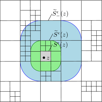
Proof.
First we consider the case where is a zero boundary GFF on . It is sufficient to establish the following two inequalities
| (A.14) |
The first inequality of (A.14) is immediate, since the number of boxes in our cover is at least as large as the number of boxes in the cover considered in [DS11, Proposition 1.6], since each -box with our definition is contained in a -box with the definition considered in [DS11].
We will now establish the second inequality of (A.14). Let denote the set of dyadic parents of squares in . With as in (A.12), define the following quantum -neighborhoods of :
For define to be the dyadic parent of , and define (resp. ) to be the -neighborhood of (resp. the -neighborhood of ), where is the side length of . The first step of our proof is to reduce the lemma (for the case of a zero boundary GFF) to proving the following estimate:
| (A.15) |
Let
By (A.16), which we will explain just below, we see that (A.15) is sufficient to prove the lemma:
| (A.16) |
The first equality of (A.16) follows by . The second estimate of (A.16) follows since for any it holds that and for at most 9 of the dyadic squares which intersect .
Our justification of (A.15) will be very brief, since a similar argument can be found in [DS11]. Let be the rooted probability measure defined in [DS11, Section 3.3]. Proceeding similarly as in [DS11], and letting denote the (random) side length of for , we see that
| (A.17) |
In particular, the first equality of (A.17) follows by the argument right after the statement of [DS11, Theorem 4.2], and the second equality of (A.17) follows by the argument of the first paragraph in the proof of [DS11, Theorem 4.2]. The last inequality of (A.17) follows by using that the dyadic squares have a side length which is smaller than or equal to the corresponding dyadic squares considered in [DS11, Section 1.4], and that the last inequality of (A.17) holds for the dyadic squares considered in [DS11]. The estimate (A.17) implies (A.15), which concludes the proof of the lemma for the case of the zero boundary GFF.
Next we consider the case where is a whole-plane GFF with additive constant chosen so that its circle average over is 0. Choose such that . Then , where is a zero boundary GFF in , and is a harmonic function in . By [GHM15, Lemma 3.12], and by using that is the circle average of around , so that is a centered Gaussian random variable with variance , for any ,
Hence, except on an event of probability , for any , we have . Since is arbitrary, the statement of the lemma for the case of a whole-plane GFF follows from the case of a zero-boundary GFF on . ∎
We will apply the following basic lemma in our proof of Proposition A.5.
Lemma A.7.
Let be the -LQG measure associated with a whole-plane GFF with additive constant chosen such that the average around is 0. Let be a bounded open set. For let be a deterministic collection of at most Euclidean balls of radius contained in , and define . Given any we can find such that , where the implicit constant is independent of .
Proof.
By [GHM15, Lemma 5.2] and the Chebyshev inequality, for any , and , we have
where . By the union bound,
If we choose then for small enough , we have , which implies the lemma. ∎
Proof of Proposition A.5.
First we consider the case where is a whole-plane GFF normalized as in the statement of the proposition. Fix a large constant to be chosen later, depending only on . For let be the event that the following is true.
-
(i)
All squares for which have Euclidean side length at least , where is chosen sufficiently large such that the probability of this event is at least . Existence of an appropriate (independent of ) follows from Lemma A.7 applied with e.g. , , and a collection of balls such that each for which is contained in a ball in , where is the set of -neighborhoods of boxes in .
-
(ii)
For any interval for which and the set contains a ball of radius at least .
By [GHM15, Proposition 3.4 and Remark 3.9], the probability of the event in (ii) is of order , at a rate depending only on and the diameter of . Hence . If the event (ii) occurs, then for any dyadic box of side length , the number of disjoint SLE segments for any interval which intersect both and is bounded by (c.f. [GHM15, Lemma 5.1]). Therefore the condition (i) implies that on the event we have . Note that for a slightly larger open set containing , so by Hölder’s inequality and the moment estimate in [RV14a, Theorem 2.11], we see that decays faster than any power of . It follows that
Since was arbitrary, an application of Lemma A.6 concludes the proof of the proposition for the case of a whole-plane GFF.
Now we assume is the circle average embedding of an -quantum cone and that lies at positive distance from 0. Let be a slightly larger domain containing which also lies at positive distance from 0. By [GHM15, Lemma 3.10], we can couple with an instance of a whole-plane GFF (normalized as above) satisfying the following property. There is a constant such that for each , it holds except on an event of probability that for each . Let (resp. ) denote the number of boxes in (3.14) when the field is (resp. ). By the coupling between and , except on an event of probability , we have . We conclude the proof of the proposition by using the above result for the whole-plane GFF (and we decrease in the very last step if necessary):
A.3 Proof of Lemma 5.3
In this section we prove our restricted sub-addivity lemma, Lemma 5.3. The following recursive relation is the key observation for the proof.
Lemma A.8.
Assume we are in the setting of Lemma 5.3. For each with , we have
Proof.
Lemma A.9.
Let be non-decreasing functions and suppose there exists such that and for . Let be a sequence of real numbers and suppose there exists a with the following property. For each sequence with and for each , we have . Then .
Proof.
For , let and be the -fold compositions of and , respectively.
Suppose that is an increasing sequence of positive integers with and for each . We claim that . To see this, we will construct a sequence with for each such that is a subsequence of . Let and for , let be chosen so that . Such an exists since so for , whence .
Since we have . Therefore . By definition of and for ,
| (A.19) |
For , let . Let . For and , let . Let . We claim that for each . Indeed, given , let be chosen so that . If , then we have , so clearly the desired inequalities hold in this case. If , then we have and . By (A.19) we have and by definition of we have , as required. Since (by hypothesis) we also have .
We now argue that . If not, we can find an increasing sequence and such that for each . By passing to a subsequence we can arrange that and for each . Then the claim above implies that , which is a contradiction. ∎
Proof of Lemma 5.3.
Fix and . For let and . Observe that and satisfy the hypotheses of Lemma A.9. By Lemma A.9 it suffices to show that there is a such that for each sequence with and for each , we have .
Fix such a sequence and let . Since , there is a such that for , we have . By Lemma A.8, for we have
Dividing by gives
| (A.20) |
Since and for each we have for each and
Since , this is summable. Let
The relation (A.20) implies that for each . Since for each , we infer that exists. Hence also
exists. It remains to show that the does not depend on the initial choice of sequence . To this end, it is enough to show that
| (A.21) |
since then the limiting values arising from two different choices of subsequence must agree by symmetry.
References
- [AB14] J. Ambjørn and T. G. Budd. Geodesic distances in Liouville quantum gravity. Nuclear Physics B, 889:676–691, December 2014, 1405.3424.
- [AHS17] J. Aru, Y. Huang, and X. Sun. Two perspectives of the 2D unit area quantum sphere and their equivalence. Comm. Math. Phys., 356(1):261–283, 2017, 1512.06190. MR3694028
- [AK16] S. Andres and N. Kajino. Continuity and estimates of the Liouville heat kernel with applications to spectral dimensions. Probab. Theory Related Fields, 166(3-4):713–752, 2016, 1407.3240. MR3568038
- [Ald91a] D. Aldous. The continuum random tree. I. Ann. Probab., 19(1):1–28, 1991. MR1085326 (91i:60024)
- [Ald91b] D. Aldous. The continuum random tree. II. An overview. In Stochastic analysis (Durham, 1990), volume 167 of London Math. Soc. Lecture Note Ser., pages 23–70. Cambridge Univ. Press, Cambridge, 1991. MR1166406 (93f:60010)
- [Ald93] D. Aldous. The continuum random tree. III. Ann. Probab., 21(1):248–289, 1993. MR1207226 (94c:60015)
- [ANR+98] J. Ambjørn, J. L. Nielsen, J. Rolf, D. Boulatov, and Y. Watabiki. The spectral dimension of 2D quantum gravity. Journal of High Energy Physics, 2:010, February 1998, hep-th/9801099.
- [Aru15] J. Aru. KPZ relation does not hold for the level lines and SLEκ flow lines of the Gaussian free field. Probab. Theory Related Fields, 163(3-4):465–526, 2015, 1312.1324. MR3418748
- [BBI01] D. Burago, Y. Burago, and S. Ivanov. A course in metric geometry, volume 33 of Graduate Studies in Mathematics. American Mathematical Society, Providence, RI, 2001. MR1835418
- [Ber07a] O. Bernardi. Bijective counting of Kreweras walks and loopless triangulations. J. Combin. Theory Ser. A, 114(5):931–956, 2007.
- [Ber07b] O. Bernardi. Bijective counting of tree-rooted maps and shuffles of parenthesis systems. Electron. J. Combin., 14(1):Research Paper 9, 36 pp. (electronic), 2007, math/0601684. MR2285813 (2007m:05125)
- [Ber15] N. Berestycki. Diffusion in planar Liouville quantum gravity. Ann. Inst. Henri Poincaré Probab. Stat., 51(3):947–964, 2015, 1301.3356. MR3365969
- [BGRV16] N. Berestycki, C. Garban, R. Rhodes, and V. Vargas. KPZ formula derived from Liouville heat kernel. J. Lond. Math. Soc. (2), 94(1):186–208, 2016, 1406.7280. MR3532169
- [BHS18] O. Bernardi, N. Holden, and X. Sun. Percolation on triangulations: a bijective path to Liouville quantum gravity. In preparation, 2018.
- [BJRV13] J. Barral, X. Jin, R. Rhodes, and V. Vargas. Gaussian multiplicative chaos and KPZ duality. Comm. Math. Phys., 323(2):451–485, 2013, 1202.5296. MR3096527
- [BS09] I. Benjamini and O. Schramm. KPZ in one dimensional random geometry of multiplicative cascades. Comm. Math. Phys., 289(2):653–662, 2009, 0806.1347. MR2506765 (2010c:60151)
- [CL14] N. Curien and J.-F. Le Gall. The Brownian plane. J. Theoret. Probab., 27(4):1249–1291, 2014, 1204.5921. MR3278940
- [dBE52] N. G. de Bruijn and P. Erdös. Some linear and some quadratic recursion formulas. II. Nederl. Akad. Wetensch. Proc. Ser. A. 55 = Indagationes Math., 14:152–163, 1952. MR0047162
- [DD16] J. Ding and A. Dunlap. Liouville first-passage percolation: subsequential scaling limit at high temperature. ArXiv e-prints, May 2016, 1605.04011.
- [DG16a] J. Ding and S. Goswami. Liouville first passage percolation: the weight exponent is strictly less than 1 at high temperatures. ArXiv e-prints, May 2016, 1605.08392.
- [DG16b] J. Ding and S. Goswami. Upper bounds on Liouville first passage percolation and Watabiki’s prediction. ArXiv e-prints, October 2016, 1610.09998.
- [DG17] J. Ding and S. Goswami. First passage percolation on the exponential of two-dimensional branching random walk. Electron. Commun. Probab., 22:Paper No. 69, 14, 2017, 1511.06932. MR3742400
- [DKRV16] F. David, A. Kupiainen, R. Rhodes, and V. Vargas. Liouville quantum gravity on the Riemann sphere. Comm. Math. Phys., 342(3):869–907, 2016, 1410.7318. MR3465434
- [DMS14] B. Duplantier, J. Miller, and S. Sheffield. Liouville quantum gravity as a mating of trees. ArXiv e-prints, September 2014, 1409.7055.
- [DRSV14] B. Duplantier, R. Rhodes, S. Sheffield, and V. Vargas. Renormalization of critical Gaussian multiplicative chaos and KPZ relation. Comm. Math. Phys., 330(1):283–330, 2014, 1212.0529. MR3215583
- [DS11] B. Duplantier and S. Sheffield. Liouville quantum gravity and KPZ. Invent. Math., 185(2):333–393, 2011, 1206.0212. MR2819163 (2012f:81251)
- [DW15a] D. Denisov and V. Wachtel. Random walks in cones. Ann. Probab., 43(3):992–1044, 2015, 1110.1254. MR3342657
- [DW15b] J. Duraj and V. Wachtel. Invariance principles for random walks in cones. ArXiv e-prints, August 2015, 1508.07966.
- [DZ15] J. Ding and F. Zhang. Non-universality for first passage percolation on the exponential of log-correlated Gaussian fields. Probability Theory and Related Fields, to appear, 2015, 1506.03293.
- [DZ16] J. Ding and F. Zhang. Liouville first passage percolation: geodesic dimension is strictly larger than 1 at high temperatures. ArXiv e-prints, October 2016, 1610.02766.
- [Eva85] S. N. Evans. On the Hausdorff dimension of Brownian cone points. Math. Proc. Cambridge Philos. Soc., 98(2):343–353, 1985. MR795899 (86j:60185)
- [GH18] E. Gwynne and T. Hutchcroft. Anomalous diffusion of random walk on random planar maps. In preparation, 2018.
- [GHM15] E. Gwynne, N. Holden, and J. Miller. An almost sure KPZ relation for SLE and Brownian motion. ArXiv e-prints, December 2015, 1512.01223.
- [GHMS17] E. Gwynne, N. Holden, J. Miller, and X. Sun. Brownian motion correlation in the peanosphere for . Ann. Inst. Henri Poincaré Probab. Stat., 53(4):1866–1889, 2017, 1510.04687. MR3729638
- [GHS17] E. Gwynne, N. Holden, and X. Sun. A mating-of-trees approach for graph distances in random planar maps. ArXiv e-prints, November 2017, 1711.00723.
- [GKMW18] E. Gwynne, A. Kassel, J. Miller, and D. B. Wilson. Active Spanning Trees with Bending Energy on Planar Maps and SLE-Decorated Liouville Quantum Gravity for . Comm. Math. Phys., 358(3):1065–1115, 2018, 1603.09722. MR3778352
- [GM17a] E. Gwynne and J. Miller. Characterizations of SLEκ for on Liouville quantum gravity. ArXiv e-prints, January 2017, 1701.05174.
- [GM17b] E. Gwynne and J. Miller. Random walk on random planar maps: spectral dimension, resistance, and displacement. ArXiv e-prints, November 2017, 1711.00836.
- [GMS17a] E. Gwynne, C. Mao, and X. Sun. Scaling limits for the critical Fortuin-Kasteleyn model on a random planar map I: cone times. Annales de l’Institut Henri Poincaré, to appear, 2017, 1502.00546.
- [GMS17b] E. Gwynne, J. Miller, and S. Sheffield. The Tutte embedding of the mated-CRT map converges to Liouville quantum gravity. ArXiv e-prints, May 2017, 1705.11161.
- [GRV14] C. Garban, R. Rhodes, and V. Vargas. On the heat kernel and the Dirichlet form of Liouville Brownian motion. Electron. J. Probab., 19:no. 96, 25, 2014, 1302.6050. MR3272329
- [GRV16] C. Garban, R. Rhodes, and V. Vargas. Liouville Brownian motion. Ann. Probab., 44(4):3076–3110, 2016, 1301.2876. MR3531686
- [GS17] E. Gwynne and X. Sun. Scaling limits for the critical Fortuin-Kasteleyn model on a random planar map II: local estimates and empty reduced word exponent. Electronic Jorunal of Probability, 22:Paper No. 45, 1–56, 2017, 1505.03375.
- [HS16] N. Holden and X. Sun. SLE as a mating of trees in Euclidean geometry. ArXiv e-prints, October 2016, 1610.05272.
- [KMSW15] R. Kenyon, J. Miller, S. Sheffield, and D. B. Wilson. Bipolar orientations on planar maps and SLE12. ArXiv e-prints, November 2015, 1511.04068.
- [KPZ88] V. Knizhnik, A. Polyakov, and A. Zamolodchikov. Fractal structure of 2D-quantum gravity. Modern Phys. Lett A, 3(8):819–826, 1988.
- [Le 07] J.-F. Le Gall. The topological structure of scaling limits of large planar maps. Invent. Math., 169(3):621–670, 2007, math/0607567. MR2336042 (2008i:60022)
- [Le 13] J.-F. Le Gall. Uniqueness and universality of the Brownian map. Ann. Probab., 41(4):2880–2960, 2013, 1105.4842. MR3112934
- [Le 14] J.-F. Le Gall. Random geometry on the sphere. Proceedings of the ICM, 2014, 1403.7943.
- [LSW17] Y. Li, X. Sun, and S. S. Watson. Schnyder woods, SLE(16), and Liouville quantum gravity. ArXiv e-prints, May 2017, 1705.03573.
- [Mie09] G. Miermont. Random maps and their scaling limits. In Fractal geometry and stochastics IV, volume 61 of Progr. Probab., pages 197–224. Birkhäuser Verlag, Basel, 2009. MR2762678 (2012a:60017)
- [Mie13] G. Miermont. The Brownian map is the scaling limit of uniform random plane quadrangulations. Acta Math., 210(2):319–401, 2013, 1104.1606. MR3070569
- [Moo28] R. L. Moore. Concerning upper semi-continuous collections of continua. Trans. Amer. Math. Soc., 27(4):416–428, 1928.
- [MRVZ16] P. Maillard, R. Rhodes, V. Vargas, and O. Zeitouni. Liouville heat kernel: regularity and bounds. Ann. Inst. Henri Poincaré Probab. Stat., 52(3):1281–1320, 2016, 1406.0491. MR3531710
- [MS15a] J. Miller and S. Sheffield. An axiomatic characterization of the Brownian map. ArXiv e-prints, June 2015, 1506.03806.
- [MS15b] J. Miller and S. Sheffield. Liouville quantum gravity and the Brownian map I: The QLE(8/3,0) metric. ArXiv e-prints, July 2015, 1507.00719.
- [MS15c] J. Miller and S. Sheffield. Liouville quantum gravity spheres as matings of finite-diameter trees. ArXiv e-prints, June 2015, 1506.03804.
- [MS16a] J. Miller and S. Sheffield. Imaginary geometry III: reversibility of SLEκ for . Annals of Mathematics, 184(2):455–486, 2016, 1201.1498.
- [MS16b] J. Miller and S. Sheffield. Liouville quantum gravity and the Brownian map II: geodesics and continuity of the embedding. ArXiv e-prints, May 2016, 1605.03563.
- [MS16c] J. Miller and S. Sheffield. Liouville quantum gravity and the Brownian map III: the conformal structure is determined. ArXiv e-prints, August 2016, 1608.05391.
- [MS16d] J. Miller and S. Sheffield. Imaginary geometry I: interacting SLEs. Probab. Theory Related Fields, 164(3-4):553–705, 2016, 1201.1496. MR3477777
- [MS16e] J. Miller and S. Sheffield. Imaginary geometry II: Reversibility of for . Ann. Probab., 44(3):1647–1722, 2016, 1201.1497. MR3502592
- [MS16f] J. Miller and S. Sheffield. Quantum Loewner evolution. Duke Math. J., 165(17):3241–3378, 2016, 1312.5745. MR3572845
- [MS17] J. Miller and S. Sheffield. Imaginary geometry IV: interior rays, whole-plane reversibility, and space-filling trees. Probab. Theory Related Fields, 169(3-4):729–869, 2017, 1302.4738. MR3719057
- [Mul67] R. C. Mullin. On the enumeration of tree-rooted maps. Canad. J. Math., 19:174–183, 1967. MR0205882 (34 #5708)
- [RV11] R. Rhodes and V. Vargas. KPZ formula for log-infinitely divisible multifractal random measures. ESAIM Probab. Stat., 15:358–371, 2011, 0807.1036. MR2870520
- [RV14a] R. Rhodes and V. Vargas. Gaussian multiplicative chaos and applications: A review. Probab. Surv., 11:315–392, 2014, 1305.6221. MR3274356
- [RV14b] R. Rhodes and V. Vargas. Spectral Dimension of Liouville Quantum Gravity. Ann. Henri Poincaré, 15(12):2281–2298, 2014, 1305.0154. MR3272822
- [Sch00] O. Schramm. Scaling limits of loop-erased random walks and uniform spanning trees. Israel J. Math., 118:221–288, 2000, math/9904022. MR1776084 (2001m:60227)
- [She07] S. Sheffield. Gaussian free fields for mathematicians. Probab. Theory Related Fields, 139(3-4):521–541, 2007, math/0312099. MR2322706 (2008d:60120)
- [She16a] S. Sheffield. Conformal weldings of random surfaces: SLE and the quantum gravity zipper. Ann. Probab., 44(5):3474–3545, 2016, 1012.4797. MR3551203
- [She16b] S. Sheffield. Quantum gravity and inventory accumulation. Ann. Probab., 44(6):3804–3848, 2016, 1108.2241. MR3572324
- [Shi85] M. Shimura. Excursions in a cone for two-dimensional Brownian motion. J. Math. Kyoto Univ., 25(3):433–443, 1985. MR807490 (87a:60095)
- [SS13] O. Schramm and S. Sheffield. A contour line of the continuum Gaussian free field. Probab. Theory Related Fields, 157(1-2):47–80, 2013, math/0605337. MR3101840
- [Wat93] Y. Watabiki. Analytic study of fractal structure of quantized surface in two-dimensional quantum gravity. Progr. Theor. Phys. Suppl., (114):1–17, 1993. Quantum gravity (Kyoto, 1992).