A Distribution Evolutionary Algorithm for the Graph Coloring Problem
Abstract
\colorblueGraph coloring is a challenging combinatorial optimization problem with a wide range of applications. In this paper, a distribution evolutionary algorithm based on a population of probability model (DEA-PPM) is developed to address it efficiently. Unlike existing estimation of distribution algorithms where a probability model is updated by generated solutions, DEA-PPM employs a distribution population based on a novel probability model, and an orthogonal exploration strategy is introduced to search the distribution space with the assistance of an refinement strategy. By sampling the distribution population, efficient search in the solution space is realized based on a tabu search process. Meanwhile, DEA-PPM introduces an iterative vertex removal strategy to improve the efficiency of -coloring, and an inherited initialization strategy is implemented to address the chromatic problem well. The cooperative evolution of the distribution population and the solution population leads to a good balance between exploration and exploitation. Numerical results demonstrate that the DEA-PPM of small population size is competitive to the state-of-the-art metaheuristics.
keywords:
distribution evolutionary algorithm, orthogonal exploration, inherited initialization, graph coloring, estimation of distribution algorithm1 Introduction
Given an undirected graph with a vertex set and a edge set , the (vertex) graph coloring problem (GCP) assigns colors to vertexes such that no adjacent vertexes share the same color. If can be colored by different colors without color conflicts, it is -colorable. The smallest value of color number such that is -colorable is its chromatic number, denoted by . There are two instances of the GCP, the -coloring problem attempting to color a graph with colors and the chromatic number problem trying to get the chromatic number of , both of which are extensively applied in scientific and engineering fields. \colorredDue to the NP-completeness of GCPs, some relaxation methods were proposed to transform the combinatorial GCPs to continuous optimization problems [1, 2, 3]. However, the transformation will lead to continuous problems with distinct landscapes, and global optimal solutions of the original GCPs could be quite different from those of the relaxed problems.
Accordingly, a variety of metaheuristics have been developed to address the original GCPs efficiently [4]. Individual-based metaheuristics search the solution space by single-point iteration schemes, contributing to their fast convergence and low complexity [5]. However, their performance relies heavily on the initial solution and the definition of neighborhood, which makes it challenging to balance the exploration and the exploitation. Population-based metaheuristics perform cooperative multi-point search in the solution space, but a comparatively large population is usually necessary for the efficient search in the solution space, which makes it inapplicable to large-scale GCPs [4].
Recently, metaheuristics based on probability models have been widely employed to solve complicated optimization problems [6, 7, 8]. As two popular instances, the ant colony optimization (ACO) [6] and the estimation of distribution algorithm (EDA) [7] employ a single probability model that is gradually updated during the iteration process, which makes it difficult to balance the global exploration and the local exploitation in the distribution space. The quantum-inspired evolutionary algorithm (QEA) performs an active update of probability model by the Q-gate rotation, whereas it is a kind of local exploitation that cannot explore the distribution space efficiently [8]. To remedy the aformentioned issues, we propose a distribution evolutionary algorithm based on a population of probability model (DEA-PPM), where a balance between the convergence performance and the computational complexity could be kept by evolution of small populations. \colorblue Contributions of this work are as follows.
-
1.
We propose a novel distribution model that incorporates the advantages of EDAs and QEAs.
-
2.
Based on the proposed distribution model, an orthogonal exploration strategy is introduced to search the probability space with the assistance of a tailored refinement strategy.
-
3.
For the chromatic problem, an inherited initialization is presented to accelerate the convergence process.
red Rest of this paper is organized as follows. Section 2 presents a brief review on related works. The proposed distribution model is presented in Section 3, and Section 4 elaborates details of DEA-PPM. Section 5 investigates the influence of parameter and the distribution evolution strategies, and the competitiveness of DEA-PPM is verified by numerical experiments. Finally, we summarize the work in Section 6.
2 Literature Review
2.1 Individual-based metaheuristics for GCPs
Besides the simulated annealing [9, 10] and the variable neighborhood search [11], the tabu search (TS) is one of the most popular individual-based metaheuristics applied to solve the GCPs [12]. Porumbel et al. [13] improved the performance of TS by evaluation functions that incorporates the structural or dynamic information in addition to the number of conflicting edges. Blöchliger and Zufferey [14] proposed a TS-based constructive strategy, which constructs feasible but partial solutions and gradually increases its size to get the optimal color assignment of a GCP. Hypothesizing that high quality solutions of GCPs could be grouped in clusters within spheres of a specific diameter, Porumbel et al. [15] proposed two improved TS variants using a learning process and a tree-like structure of the connected spheres. Assuming that each vertex only interacts with a limited number of components, Galán [16] developed a decentralized coloring algorithm, where colors of vertexes are modified according to those of the adjacent vertexes to iteratively reduce the number of edge conflicts. Sun et al. [17] established a solution-driven multilevel optimization framework for GCP, where an innovative coarsening strategy that merges vertexes based on the solution provided by the TS, and the uncoarsening phase is performed on obtained coarsened results to get the coloring results of the original graph. To color vertexes with a given color number , Peng et al. [18] partitioned a graph into a set of connected components and a vertex cut component, and combined the separately local colors by an optimized maximum matching based method.
Since a probability model can provide a bird’s-eye view for the landscape of optimization problem, Zhou et al. [19, 20] proposed to enhance the global exploration of individual-based metaheuristics by the introduction of probability models. They deployed a probabilistic model for the colors of vertexes, which is updated with the assistance of a reinforcement learning technology based on discovered local optimal solutions [19]. Moreover, they improved the learning strategy of probability model to develop a three-phase local search, that is, a starting coloring generation phase based on a probability matrix, a heuristic coloring improvement phase and a learning based probability updating phase [20].
2.2 Population-based metaheuristics for GCPs
Population-based iteration mechanisms are incorporated to the improve exploration abilities of metaheuristics as well. Hsu et al. [21] proposed a modified turbulent particle swarm optimization algorithm for the planar graph coloring problem, where a three-stage turbulent model is employed to strike a balance between exploration and exploitation. Hernández and Blum [22] dealt with the problem of finding valid graphs colorings in a distributed way, and the assignment of different colors to neighboring nodes is asynchronously implemented by simulating the calling behavior of Japanese tree frogs. Rebollo-Ruiz and M. Graña [23] addressed the GCP by a gravitational swarm intelligence algorithm, where nodes of a graph are mapped to agents, and its connectivity is mapped into a repulsive force between the agents corresponding to adjacent nodes. Based on the conflict matrices of candidate solutions, Zhao et al. [24] developed a dimension-by-dimension update method, by which a discrete selfish herd optimizer was proposed to address GCPs efficiently. Aiming to develop an efficient parameter-free algorithm, Chalupa and Nielsen [25] proposed to improve the global exploration by a multiple cooperative searching strategy. For the four-colormap problem, Zhong et al. [26] proposed an enhanced discrete dragonfly algorithm that performs a global search and a local search alternately to color maps efficiently.
The incorporation of probability models are likewise employed to improve the performance of population-based metaheuristics. Bui et al. [27] developed a constructive strategy of coloring scheme based on an ant colony, where an ant colors just a portion of the graph unsing only local information. Djelloul et al. [28] took a collection of quantum matrices as the population of the cuckoo search algorithm, and an adapted hybrid quantum mutation operation was introduced to get enhanced performance of the cuckoo search algorithm.
2.3 Hybrid metaheuristics for GCPs
The population-based metaheuristics can be further improved by hybrid search strategies. Paying particular attention to ensuring the population diversity, Lü and Hao [29] proposed an adaptive multi-parent crossover operator and a diversity-preserving strategy to improve the searching efficiency of evolutionary algorithms, and proposed a memetic algorithm that takes the TS as a local search engine. Porumbel et al. [30] developed a population management strategy that decides whether an offspring should be accepted in the population, which individual needs to be replaced and when mutation is applied. Mahmoudi and Lotfi [31] proposed a discrete cuckoo optimization algorithm for the GCP, where a neighborhood search in radius of the lay egg causes the algorithm hardly trapped in local minimum and producing new eggs. Accordingly, it provides a good balance between diversification and centralizing.
Wu and Hao [32] proposed a preprocessing method that extracts large independent sets by the TS, and the memetic algorithm proposed by Lü and Hao [29] was employed to color the residual graph. For the chromatic problem, Douiri and Elbernoussi [33] initialized the color number by the coloring result of a heuristic algorithm and generated the initial population of genetic algorithm (GA) by finding a maximal independent set approximation of the investigated graph.
Bessedik et al. [34] addressed the GCPs within the framework of the honey bees optimization, where a local search, a tabu search and an ant colony system are implemented as workers and queens are randomly generated. Mirsaleh and Meybodi [35] proposed a Michigan memetic algorithm for GCPs, where each chromosome is associated to a vertex of the input graph. Accordingly, each chromosome is a part of the solution and represents a color for its corresponding vertex, and each chromosome locally evolves by evolutionary operators and improves by a learning automata based local search. Moalic and Gondran [36] integrated a TS procedure with an evolutionary algorithm equipped with the greedy partition crossover, by which the hybrid algorithm can performs well with a population consisting of two individuals. Silva et al. [37] developed a hybrid algorithm iColourAnt, which addresses the GCP using an ant colony optimization procedure with assistance of a local search performed by the reactive TS.
2.4 Related work on the estimation of distribution algorithm
A large number of works have been reported to improve the general performance of EDAs. To improve the general precision of a distribution model, Shim et al. [38] modelled the restricted Boltzmann machine as a novel EDA, where the probabilistic model is constructed using its energy function, and the -means clustering was employed to group the population into small clusters. Approximating the Boltzmann distribution by a Gaussian model, Valdez et al. [39] proposed a Boltzmann univariate marginal distribution algorithm, where the Gaussian distribution obtains a better bias to sample intensively the most promising regions. Considering the multivariate dependencies between continuous random variables, PourMohammadBagher et al. [40] proposed a parallel model of some subgraphs with a smaller number of variables to avoid complex approximations of learning a probabilistic graphical model. Dong et al. [41] proposed a latent space-based EDA, which transforms the multivariate probabilistic model of Gaussian-based EDA into its principal component latent subspace of lower dimensionality to improve its performance on large-scale optimization problems.
To enhance the local exploitation of an EDA, Zhou et al. [42] suggested to combine an estimation of distribution algorithm with cheap and expensive local search methods for making use of both global statistical information and individual location information. Considering that the random sampling of Gaussian EDA usually suffers from the poor diversity and the premature convergence, Dang et al. [43] developed an efficient mixture sampling model to achieve a good tradeoff between the diversity and the convergence, by which it can explore more promising regions and utilize the unsuccessful mutation vectors.
The performance of EDA can also improved by designing tailored update strategies of the probability model. To address the multiple global optima of multimodal problem optimizations, Pẽna et al. [44] introduced the unsupervised learning of Bayesian metwokrs in EDA, which makes it able to model simultaneously the different basins represented by the selected individuals, whereas preventing genetic drift as much as possible. Peng et al. [45] developed an explicit detection mechanism of the promising areas, by which function evaluations for exploration can be significantly reduced. To prevent the Gaussian EDAs from premature convergence, Ren et al. [46] proposed to tune the main search direction by the anisotropic adaptive variance that is scaled along different eigendirections based on the landscape characteristics captured by a simple topology-based detection method. Liang et al. [47] proposed to archive a certain number of high-quality solutions generated in the previous generations, by which fewer individuals are needed in the current population for model estimation. In order to address the mixed-variable newsvendor problem, Wang et al. [48] developed a histogram model-based estimation of distribution algorithm, where an adaptive-width histogram model is used to deal with the continuous variables and a learning-based histogram model is applied to deal with the discrete variables. Liu et al. [49] embedded within the search procedure a learning mechanism based on an incremental Gaussian mixture model, by which all new solutions generated during the evolution are fed incrementally into the learning model to adaptively discover the structure of the Pareto set of an MOP.
3 The Distribution Model for the Graph Coloring Problem
3.1 The graph coloring problem
Let be the vertex number of a graph . An assignment of vertexes with colors can be represented by an integer vector , where denotes the assigned color of vertex . Then, the -coloring problem can be modelled as a minimization problem
| (1) |
While , the adjacent vertexes and are assigned with the same color, and is called a conflicting edge. Accordingly, the objective values represents the total conflicting number of the color assignment . While is -colorable, there exists an optimal partition such that , and is called a legal -color assignment of graph . Thus, the chromatic problem is modelled as
| (2) |
where represents a legal -color assignment that is an optimal color assignment of problem (1).
red
3.2 The Q-bit model and the Q-gate transformation
Different from the ACO and the EDA, the QEA employs a quantum matrix for probabilistic modelling of the solution space, modelling the probability distribution of a binary variable by a Q-bit satisfying [50]. That is, and give the probabilities of and , respectively. Accordingly, the probability distribution of an -dimensional binary vector is represented by
where , . Then, the value of can be obtained by sampling the probability distribution .
The probability distribution of binary variable is modified in the QEA by the Q-gate, a orthogonal matrix
Premultiplying by , the probability distribution of is modified as
To coloring a graph of vertexes by colors, Djelloul et al. [28] modelled the probability distribution of color assignment by a quantum matrix
where
In this way, the Q-gate can be deployed for each unit vector to regulate the distribution of color assignment.
3.3 The proposed distribution model of color assignment
Since the unit vector models each candidate color of vertex independently, the sampling process would lead to multiple assignments for vertex , and an additional repair strategy is needed to get a feasible -coloring assignment [28]. To address this defect, we propose to model the color distribution of vertex by a -dimensional unit vector , and present the color distribution of vertexes as
| (3) |
where satisfies
| (4) |
The distribution model confirmed by (3) and (4) incorporates the advantages of models in EDAs and QEAs.
-
1.
An feasible -coloring of vertexes can be achieved by successively sampling columns of .
-
2.
The update of probability distribution can be implemented by both orthogonal transformations performed on column vectors of and direct manipulations of components that do not change the norms of columns vectors 111Details for the update process are presented in Section 4.4..
4 A Distribution Evolutionary Algorithm Based on a Population of Probability Model
blue
The proposed DEA-PPM solves the GCP based on a distribution population and a solution population. The distribution population consists of individuals representing distribution models of graph coloring, which are updated by an orthogonal exploration strategy and an composite exploitation strategy. Meanwhile, an associated solution population is deployed to exploit the solution space by the TS-based local search. Moreover, an iterative vertex removal strategy and a tailored inherited initialization strategy are introduced to accelerate the procedure of -coloring, which in turn contributes to its high efficiency of addressing the chromatic problem. Thanks to the cooperative interplay between the distribution population and the solution population, the DEA-PPM with small populations is expected to achieve competitive results of GCPs.
4.1 The framework of DEA-PPM
red As presented in Algorithm 1, DEA-PPM is implemented as two nested loops: the inner loop addressing the -coloring problem and the outer loop decreasing to get the chromatic number . Based on a distribution population and the corresponding solution population , it starts with the initialization of the color number , which is then minimized by the outer loop to get the chromatic number .
Each iteration of the outer loop begins with the iterative vertex removal (IVR) strategy [51], by which the investigated graph could be transformed into a reduced graph , and the complexity of the coloring process could be reduced as well. Then, Lines 5-11 of Algorithm 1 initialize a distribution population and the corresponding solution population for . Once is colored by Lines 12-20 of Algorithm 1, DEA-PPM recovers the obtained color assignment to get an color assignment of , and as well as is archived for the inherited initialization performed at the next generation. Repeating the aforementioned process until the termination-condition 1 is satisfied, DEA-PPM returns a color number and the corresponding color assignment .
After the initialization of , , and , the inner loop tries to get a legal -coloring assignment for the reduced graph by evolving both the distribution population and the solution population . It first performs the orthogonal exploration on to generate , and then, generates an intermediate solution population , which is further refined to get . Meanwhile, is generated by refining . The inner loop repeats until the termination-condition 2 is satisfied.
The outer loop of DEA-PPM is implemented only once for the -coloring problem. To address the chromatic problem, the termination condition 1 is satisfied if the chromatic number has been identified or the inner loop fails to get a legal -coloring assignment for a given iteration budget. The termination condition 2 is met while a legal -coloring assignment is obtained or the maximum iteration number is reached.
For the -coloring problem, DEA-PPM initializes the color number by a given positive integer. While it is employed to address the chromatic number problem, we set 222Here is the maximum vertex degree of graph . because an undirected graph is sure to be -colorable [52].
4.2 The iterative vertex removal strategy and the inverse recovery strategy
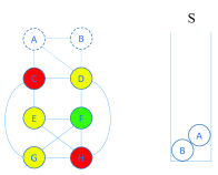
To reduce the time complexity of the -coloring algorithm, Yu et al. [51] proposed an iterative vertex removal (IVR) strategy to reduce the size of the investigated graph. By successively removing vertexes with degrees less than , IVR generates a reduced graph , and put the removed vertexes into a stack . In this way, one could get a graph where degrees of vertexes are greater than or equal to , and its size could be significantly smaller than that of .
While a -coloring assignment is obtained for the reduced graph , the inverse recovery (IR) operation is implemented by recovering vertexes in the stack . The IR process is initialized by assigning any legal color to the vertex at the top of . Because the IVR process removes vertexes with degree less than , the IR process can get all recovered vertexes colored without conflicting. An illustration for the implement of the IVR and the IR is presented in Fig. 1.


4.3 Population initialization
Depending on the iteration stage of DEA-PPM, the initialization of populations is implemented by the uniform initialization or the inherited initialization.
At the beginning, the uniform initialization generates individuals of as
| (5) |
are generated by sampling model (5) times.
While , the inherited initialization gets and with the assistance of the distribution populations and the solution population archived at the last generation. The graph has been colored with colors, and it is anticipated to get a legal -color assignment. To get an initial color assignment of colors, a color index that corresponds to the minimum vertex independent set is identified for . Then, we get the initial color assignment by
Meanwhile, delete the -th row of , and normalize its columns to get an initial distribution corresponding to colors. Details of the inherited initialization are presented in Algorithm 2.
4.4 Evolution of the distribution population
Based on the distribution model defined by (3) and (4), DEA-PPM performs the orthogonal exploration on individuals of to explore the probability space. Moreover, distribution individuals of are refined by an exploitation strategy or a disturbance strategy.
4.4.1 Orthogonal transformation
An orthogonal transformation on a column vector is performed by premultiplying an orthogonal matrix , a square matrix satisfying
where is the identity matrix. Because an orthogonal transformation preserves the 2-norm [53], we know
| (6) |
Then, by performing orthogonal transformations on columns of the distribution individuals, DEA-PPM can explore the distribution space flexibly.
4.4.2 Orthogonal exploration in the distribution space
To perform the orthogonal exploration in the distribution space, DEA-PPM generates an orthogonal matrix by performing the QR decomposition on an invertible matrix that is generated randomly. As presented in Algorithm 3, worst individuals of are modified by random orthogonal transformations performed on randomly selected columns. As an initial study, is set as a random integer in , and is an integer randomly sampled in .
4.4.3 Refinement of the distribution population
As presented in Algorithm 4, the distribution population is refined to generate . , DEA-PPM refines its -th column with the assistance of the -th components of and . With probability , is refined by an exploitation strategy; otherwise, its refinement is implemented by a disturbance strategy.
The exploitation strategy
Similar to the probability learning procedure proposed in [20], the first phase of the exploitation strategy is implemented by
| (7) |
where is the -th component of . Then, an local orthogonal transformation is performed as
| (8) |
where
, . Equation (7) conducts an overall regulation controlled by the parameter , and equation (8) rotates the subvector counterclockwise by to regulate it slightly.
The disturbance strategy
, is generated by
| (9) |
. For , the -th components of is smaller than that of , and others are greater. Thus, we set to prevent DEA-PPM from premature convergence.
4.5 Efficient search in the solution space
To search the solution space efficiently, DEA-PPM generates a solution population by sampling with inheritance, and then, refines it using a multi-parent crossover operation followed by the TS search proposed in Ref. [55].
4.5.1 The strategy of sampling with inheritance
Inspired by the group selection strategy [19], components of new solution are either generated by sampling the distribution or inheriting from the corresponding solution . The strategy of sampling with inheritance is presented in Algorithm 5, where is the probability of generating by sampling .
4.5.2 Refinement of the solution population
The quality of generated solutions is further improved by a refinement strategy presented in Algorithm 6, which is an iterative process consisting of a multi-parent greedy partition crossover guided by two promising solutions and as well as the TS process presented in Ref. [55]. Meanwhile, two promising solutions and are updated. The refinement process ceases once it stagnates for 20 consecutive iterations.
Multi-parent greedy partition crossover (MGPX)
Inspired by the motivation of greedy partition crossover (GPX) for graph coloring [55], we propose the multi-parent greedy partition crossover (MGPX) presented in Algorithm 7. For , two mutually different solutions and are selected from . Then, the MGPX is performed on , and to generate a new solution . After the traversal of the solution population , all generated solutions construct the intermediate solution population .
Update of the promising solutions
The promising solution is updated if a better solution is obtained. Then, is set as the original values of . To fully exploits the promising information incorporated by , it is updated once every 10 iterations.
5 Numerical Experiments
red The investigated algorithms are evaluated on the benchmark instances from the second DIMACS competition333Publicly available at ftp://dimacs.rutgers.edu/pub/challenge/graph/benchmarks/color/. that were used to test graph coloring algorithms in recent studies [16, 17, 20, 29, 36] . All tested algorithms are developed in C++ programming language, and run in Microsoft Windows 7 on a laptop equipped with the Intel(R) Core(TM) i7 CPU 860 @ 2.80GHz and 8GB system memory. We first perform a parameter study to get appropriate parameter settings of DEA-PPM, and then, the proposed evolution strategies of distribution population are investigated to demonstrate their impacts on its efficiency. Finally, numerical comparisons for both the chromatic problem and the -coloring problem are performed with the state-of-the-art algorithms. For numerical experiments, time budgets of all algorithms are consistently set as 3600 seconds (one hour). \colorred Because performance of the investigated algorithms varies for the selected benchmark problems, we perform the numerical comparison in two different ways. If two compared algorithms achieve inconsistent coloring results for the chromatic problem, numerical comparison is performed by the obtained color numbers; otherwise, we take the running time as the evaluation metric while they get the same coloring results.
5.1 Parameter study
By setting as the best known color numbers of the benchmark problems, preliminary experiments for the -coloring problem show that the performance of DEA-PPM is significantly influenced by the population size , the regulation parameter and the maximum iteration budget of the TS. Then, we first demonstrate the univariate influence of parameters by the one-way analysis of variance (ANOVA), and then, perform a descriptive comparison to get a set of parameter for further numerical investigations. \colorblue The benchmark instances selected for the parameter study are the -coloring problems of DSJC500.5, flat300_28_0, flat1000_50_0, flat1000_76_0, le450_15c, le450_15d.
red
5.1.1 Analysis of variance on the impacts of parameters
Our preliminary experiments show that DEA-PPM achieves promising results with , and , which is taken as the baseline parameter setting of the one-side ANOVA test of running time. With the significance level of 0.05, the significant influences are highlighted in Tab.1 by bold P-values.
| Tested Parameter | P Values | ||||||
|---|---|---|---|---|---|---|---|
| Parameter | Settings | flat300_28_0 | le450_15c | le450_15d | DSJC500.5 | flat1000_50_0 | flat1000_76_0 |
| 0.162 | 0.548 | 0.404 | 0.004 | 0.001 | 0.001 | ||
| 0.622 | 0.643 | 0.357 | 0.003 | 0.268 | 0.000 | ||
| 0.025 | 0.146 | 0.000 | 0.040 | 0.000 | 0.000 | ||
Generally, the univariate changes of , and do not have significant influence on performance of DEA-PPM for instances flat300_28_0, le450_15c and le450_15d, except that values of has great impact on the results of le450_15d. But for instances DSJC500.5, flat1000_50_0 and flat1000_76_0, the influence is significant, except that does not significantly influence the performance of DEA-PPM on flat1000_50_0. To illustrate the results, we included the curves of expected running time in Fig. 2. The univariate analysis shows that the best results could be achieved by setting , and .


5.1.2 Descriptive statistics on the composite impacts of parameters
Besides the one-way ANOVA test, we also present a descriptive comparison for the composite impact of sevaral parameter settings. With the parameter combinations presented in Tab. 2, statistical results for running time of independent runs are included in Fig. 3.
| Parameter | Setting | |||||||||||
|---|---|---|---|---|---|---|---|---|---|---|---|---|
| 4 | 4 | 4 | 4 | 4 | 4 | 8 | 8 | 8 | 8 | 8 | 8 | |
| 0.1 | 0.1 | 0.1 | 0.2 | 0.2 | 0.2 | 0.1 | 0.1 | 0.1 | 0.2 | 0.2 | 0.2 | |
| 5000 | 10000 | 20000 | 5000 | 10000 | 20000 | 5000 | 10000 | 20000 | 5000 | 10000 | 20000 | |


It indicates that the parameter setting leads to the most promising results of DEA-PPM. Combining it with the setting of other parameters, we get the parameter setting of DEA-PPM presented in Tab. 3, which is adopted in the following experiments.
5.2 Experiments on the evolution strategies of probability distribution
In DEA-PPM, the evolution of distribution population is implemented by the orthogonal exploration strategy and the exploitation strategy. We try to validate the positive effects of these strategies in this section.


To validate the efficiency of the orthogonal exploration strategy, we compare two variants, the DEA-PPM with orthogonal exploration (DEA-PPM-O) and the DEA-PPM without orthogonal exploration (DEA-PPM-N), and show in Fig. 4 the statistical results of running time for -coloring of the easy benchmark problems (DSJC500.1 (), le450_15c (), led450_15d ()) and the hard benchmark problems(DSJC500.5 (), DSJC1000.1 (), DSJC1000.9 ()). The box plots imply that with the employment of the orthogonal exploration strategy, DEA-PPM-O performs generally better than DEA-PPM-N, resulting in smaller values of the median value, the quantiles and the standard deviations of running time.
red The positive impact of exploitation strategy is verified by comparing the DEA-PPM with exploitation (DEA-PPM-E) with the variant without exploitation (DEA-PPM-W), and the box plots of running time are included in Fig. 5. It is demonstrated that DEA-PPM-E generally outperforms DEA-PPM-W in terms of the median value, the quantiles and the standard deviation of running time.


blue Besides the statistical comparison regarding the exact values of running time, we perform a further comparison by the Wilcoxon rank sum test with a significance level of 0.05, where the statistical test is based on the sorted rank of running time instead of its exact values. The results are included in Tab. 4, where “P” is the p-value of hypothesis test. For the test conclusion “R”, “+”, “-” and “” indicate that the performance of DEA-PPM is better than, worse than and incomparable to that of the compared variant, respectively. The results demonstrate that DEA-PPM outperforms DEA-PPM-N and DEA-PPM-W on two instances, and is not inferior to them for all benchmark problems. It further validates the conclusion that both the exploration strategy and the exploitation strategy significantly improve the performance of DEA-PPM.
| Instance | DEA-PPM-N | DEA-PPM-W | ||
|---|---|---|---|---|
| P | R | P | R | |
| DSJC500.1 | 1.08E-01 | 9.25E-01 | ||
| le450_15c | 6.36E-01 | 4.99E-02 | + | |
| le450_15d | 2.50E-01 | 7.76E-01 | ||
| DSJC500.5 | 4.97E-02 | + | 5.29E-02 | |
| DSJC1000.1 | 6.56E-03 | + | 4.57E-01 | - |
| DSJC1000.9 | 7.15E-01 | 4.68E-05 | + | |
| +//- | 2/4/0 | 2/4/0 | ||
5.3 Numerical comparison with the state-of-the-art algorithms
To demonstrate the competitiveness of DEA-PPM, we perform numerical comparison for the chromatic problem and the -coloring problem with SDGC [16], MACOL [29], SDMA [17], PLSCOL [20], and HEAD [36], the parameter settings of which are presented in Tab. 5. If an algorithm cannot address the chromatic problem or the -coloring problem in 3600 seconds, a failed run is recorded by the running time of 3600 seconds.
| Algorithms | Parameters | Description | Values |
| SDGC | The number of iterations; | ||
| MACOL | Size of population; | ||
| Depth of TS; | |||
| Number of parents for crossover; | A random number in | ||
| Probability for accepting worse offspring; | |||
| Parameter for goodness score function; | |||
| SDMA | Search depth of weight tabu coloring; | ||
| Tabu tenure of weight tabu coloring; | |||
| Tabu tenure of perturbation; | |||
| Level limit of coarsening phase; | |||
| Unimproved consecutive rounds for best solution; | |||
| PLSCOL | Noise probability; | ||
| Reward factor for correct group; | |||
| Penalization factor for incorrect group; | |||
| Compensation factor for expected group; | |||
| Smoothing coefficient; | |||
| Smoothing threshold; | |||
| HEAD | Depth of TS; | ||
| The number of generations into one cycle; |
5.3.1 Comparison for the chromatic number problem
In order to verify the competitiveness of DEA-PPM on the chromatic number problem, we compare it with SDGC, MACOL, SDMA, PLSCOL and HEAD by 8 selected benchmark problems, and the statistical results of 30 independent runs are collected in Tab. 6, where , , and represent the average color number, the maximum color number, the minimum color number and the standard deviation of color numbers, respectively. The best results are highlighted by bold texts.
| Instance | Algorithm | Instance | Algorithm | ||||||||||
|---|---|---|---|---|---|---|---|---|---|---|---|---|---|
| fpsol2_i_2 | 30 | SDGC | 85.4 | 79 | 91 | 3.71 | le450_15c | 15 | SDGC | 29.07 | 28 | 32 | 1.46 |
| MACOL | 88.3 | 88 | 89 | 0.46 | MACOL | 19.4 | 18 | 21 | 1.2 | ||||
| SDMA | 59.41 | 53 | 73 | 6.22 | SDMA | 30.93 | 28 | 38 | 3.12 | ||||
| PLSCOL | 73 | 71 | 77 | 1.75 | PLSCOL | 16.1 | 15 | 17 | 0.4 | ||||
| HEAD | 74.7 | 71 | 78 | 1.97 | HEAD | 15.87 | 15 | 16 | 0.34 | ||||
| DEA-PPM | 30 | 30 | 30 | 0 | DEA-PPM | 15 | 15 | 15 | 0 | ||||
| fpsol2_i_3 | 30 | SDGC | 85.5 | 79 | 95 | 4.35 | le450_15d | 15 | SDGC | 30.27 | 27 | 34 | 2.24 |
| MACOL | 88 | 87 | 89 | 0.45 | MACOL | 18.7 | 17 | 21 | 1.35 | ||||
| SDMA | 57.86 | 51 | 65 | 5.28 | SDMA | 32.72 | 31 | 38 | 2.17 | ||||
| PLSCOL | 71.67 | 66 | 77 | 3.47 | PLSCOL | 16.33 | 16 | 17 | 0.47 | ||||
| HEAD | 75.57 | 73 | 78 | 1.54 | HEAD | 15.93 | 15 | 16 | 0.25 | ||||
| DEA-PPM | 30 | 30 | 30 | 0 | DEA-PPM | 15 | 15 | 15 | 0 | ||||
| flat300_26_0 | 26 | SDGC | 40.5 | 38 | 44 | 1.5 | DSJC500_1 | 12 | SDGC | 16.67 | 16 | 18 | 0.79 |
| MACOL | 31.8 | 31 | 32 | 0.4 | MACOL | 13 | 13 | 13 | 0 | ||||
| SDMA | 44.83 | 43 | 51 | 3.12 | SDMA | 20.76 | 17 | 29 | 3.39 | ||||
| PLSCOL | 26 | 26 | 26 | 0 | PLSCOL | 12.77 | 12 | 13 | 0.42 | ||||
| HEAD | 26 | 26 | 26 | 0 | HEAD | 13 | 13 | 13 | 0 | ||||
| DEA-PPM | 26 | 26 | 26 | 0 | DEA-PPM | 12 | 12 | 12 | 0 | ||||
| flat300_28_0 | 28 | SDGC | 40.83 | 40 | 42 | 0.58 | DSJC1000_1 | 20 | SDGC | 31.63 | 31 | 32 | 0.48 |
| MACOL | 32 | 32 | 32 | 0 | MACOL | 80.37 | 76 | 82 | 2.79 | ||||
| SDMA | 45.72 | 43 | 54 | 3.64 | SDMA | 86.21 | 73 | 94 | 5.55 | ||||
| PLSCOL | 31 | 30 | 32 | 0.73 | PLSCOL | 21 | 21 | 21 | 0 | ||||
| HEAD | 31 | 31 | 31 | 0 | HEAD | 21 | 21 | 21 | 0 | ||||
| DEA-PPM | 31 | 31 | 31 | 0 | DEA-PPM | 21 | 21 | 21 | 0 |
redIt is shown that DEA-PPM generally outperforms the other five state-of-the-art algorithms on , , and of 30 independent runs. Attributed to the population-based distribution evolution strategy, the global exploration ability of DEA-PPM is enhanced significantly. Moreover, the inherited initialization strategy improve the searching efficiency of the inner loop for search of -coloring assignment. As a result, it can address these problems efficiently and obtain with a 100% success rate for all of eight selected problems.
It is noteworthy that the competitiveness is partially attributed to the IVR strategy introduced by DEA-PPM, especially for the sparse benchmark graphs fpsol2.i.2 and fpsol2.i.3. Numerical implementation shows that when , introduction of the IVR strategy reduces the vertex number of fpsol2.i.2 and fpsol2.i.3 from 451 and 425 to 90 and 88, respectively. Thus, the scale of the reduced graph is significantly cut down for fpsol2.i.2 and fpsol2.i.3, which greatly improves the efficiency of the -coloring process validated by the inner loop of DEA-PPM.
red However, it demonstrates that DEA-PPM, PLSCOL and HEAD get consistent results on the instances flag300_26_0 and DSJC1000_1, and the best results of DEA-PPM and HEAD is a bit worse than that of PLSOCL. Accordingly, we further compare their performance by the Wilcoxon rand sum test. If the compared algorithms obtain different results of color number, the sorted rank is calculated according to the color number; while they get consistent results of color number, the rank sum test is performed according to the running time of 30 independent runs.
| Instance | SDGC | MACOL | SDMA | PLSCOL | HEAD | |||||
|---|---|---|---|---|---|---|---|---|---|---|
| P | R | P | R | P | R | P | R | P | R | |
| fpsol2_i_2 | 1.09E-12 | + | 2.90E-13 | + | 1.13E-12 | + | 9.96E-13 | + | 1.11E-12 | + |
| fpsol2_i_3 | 1.17E-12 | + | 1.59E-13 | + | 1.13E-12 | + | 1.12E-12 | + | 1.03E-12 | + |
| flat300_26_0 | 7.98E-13 | + | 1.55E-13 | + | 1.11E-12 | + | 4.81E-11 | - | 6.73E-01 | |
| flat300_28_0 | 4.27E-13 | + | 1.69E-14 | + | 1.05E-12 | + | 6.31E-01 | 0.028 | + | |
| le450_15c | 8.93E-13 | + | 7.31E-13 | + | 1.13E-12 | + | 2.05E-10 | + | 1.97E-11 | + |
| le450_15d | 1.05E-12 | + | 5.16E-13 | + | 9.63E-13 | + | 3.37E-13 | + | 7.15E-13 | + |
| DSJC500_1 | 6.21E-13 | + | 1.69E-14 | + | 9.31E-13 | + | 1.47E-09 | + | 1.69E-14 | + |
| DSJC1000_1 | 3.80E-13 | + | 1.09E-12 | + | 1.15E-12 | + | 2.74E-11 | - | 3.73E-09 | - |
| +//- | 8/0/0 | 8/0/0 | 8/0/0 | 5/1/2 | 6/1/1 | |||||
The test results demonstrate that DEA-PPM does outperform SDGC, MACOL and SDMA on the selected benchmark problems. For the instance flat300_26_0, it is shown in Tab. 6 that DEA-PPM, PLSCOL and HEAD can address the chromatic number in 3600s. While the running time is compared by the rank sum test, we get the conclusion that PLSCOL runs fast than DEA-PPM. Considering the instance DSJC1000_1, DEA-PPM, PLSCOL and HEAD stagnate at the assignment of 21 colors. However, the rank sum test shows that DEA-PPM is inferior to PLSCOL and HEAD in term of the running time.
5.3.2 Comparison for the -coloring problem
Numerical results on the chromatic problem imply that DEA-PPM, PLSCOL and HEAD outperform SDGC, MACOL and SDMA, but the superiority of DEA-PPM over PLSCOL and HEAD is dependent on the benchmark instances. To further compare DEA-PPM with PLSCOL and HEAD, we investigate their performance for the -coloring problem, where is set as the chromatic number of the investigate instance. For 18 selected benchmark problems collected in Tab. 8, we present the success rate (SR) and average runtime (T) of 30 independent runs, and the best results are highlighted by bold texts.
| Instance | PLSCOL | HEAD | DEA-PPM | ||||
|---|---|---|---|---|---|---|---|
| SR | T(s) | SR | T(s) | SR | T(s) | ||
| DSJC125.5 | 17 | 30/30 | 0.31 | 30/30 | 0.55 | 30/30 | 0.65 |
| DSJC125.9 | 44 | 30/30 | 0.08 | 30/30 | 0.12 | 30/30 | 0.39 |
| DSJC250.5 | 28 | 30/30 | 17.60 | 30/30 | 37.03 | 30/30 | 23.93 |
| DSJC250.9 | 72 | 30/30 | 6.22 | 30/30 | 7.20 | 30/30 | 42.97 |
| DSJC500.1 | 12 | 9/30 | 3140.21 | 29/30 | 1655.11 | 30/30 | 226.14 |
| DSJC500.5 | 48 | 0/30 | 3600 | 30/30 | 1176.30 | 30/30 | 771.39 |
| DSJC500.9 | 126 | 0/30 | 3600 | 1/30 | 3504.49 | 3/30 | 3346.64 |
| DSJC1000.1 | 20 | 0/30 | 3600 | 0/30 | 3600 | 30/30 | 902.53 |
| DSJC1000.5 | 85 | 0/30 | 3600 | 30/30 | 2575.73 | 23/30 | 2271.70 |
| DSJC1000.9 | 225 | 0/30 | 3600 | 19/30 | 2784.67 | 12/30 | 3240.40 |
| le450_15c | 15 | 0/30 | 3600 | 30/30 | 400.85 | 30/30 | 9.34 |
| le450_15d | 15 | 0/30 | 3600 | 27/30 | 1121.86 | 30/30 | 24.60 |
| flat300_20_0 | 20 | 30/30 | 0.11 | 30/30 | 0.20 | 30/30 | 0.81 |
| flat300_26_0 | 26 | 30/30 | 3.47 | 30/30 | 8.81 | 30/30 | 15.46 |
| flat300_28_0 | 30 | 5/30 | 3196.66 | 0/30 | 3600 | 0/30 | 3600 |
| flat1000_50_0 | 50 | 30/30 | 159.32 | 30/30 | 433.27 | 30/30 | 636.96 |
| flat1000_60_0 | 60 | 30/30 | 347.74 | 30/30 | 580.71 | 30/30 | 843.81 |
| flat1000_76_0 | 84 | 0/30 | 3600 | 23/30 | 2834.23 | 30/30 | 2139.33 |
| Average Rank | 1.94 | 2 | 1.38 | 2.05 | 1.16 | 1.83 | |
blue Thanks to the incorporation of the population-based distribution evolution strategy, the global exploration of DEA-PPM has been significantly improved, resulting in better success rate for most of the selected problems except for DSJC1000.9 and flag_300_28_0. Accordingly, the average rank of DEA-PPM is 1.16, better than 1.94 of PLSCOL and 1.38 of HEAD. The global exploration improved by the population-based distribution strategy and the IVR contributes to faster convergence of DEA-PPM for the complicated benchmark problems, however, increases the generational complexity of DEA-PPM, which leads to its slightly increased running time in some small-scale problems. Consequently, DEA-PPM gets the first place with the average running-time rank 1.83.
redFurther investigation of the performance is conducted by the Wilcoxon rank sum test of running time. With a significance level of 0.05, the results are presented in Tab. 9, where “P” is the p-value of hypothesis test. While both HEAD and DEA-PPM cannot get legal color assignments for flat300_28_0, the Wilcoxon rank sum test is conducted by the numbers of conflicts of 30 independent runs.
It is shown that DEA-PPM performs better than PLSCOL for 2 of 9 selected instances with vertex number less than 500, and better than HEAD for 3 of 9 problems, but performs a bit worse than PLSCOL and HEAD for most of small-scale instances. However, It outperforms PLSCOL and HEAD on the vast majority of instances with vertex number greater than or equal to 500. Therefore, we can conclude that DEA-PPM is competitive to PLSCOL and HEAD on large-scale GCPs, which is attributed to the composite function of the population-based distribution evolution mechanism and the IVR strategy.
| Instance () | PLSCOL | HEAD | Instance () | PLSCOL | HEAD | ||||
|---|---|---|---|---|---|---|---|---|---|
| P | R | P | R | P | R | P | R | ||
| DSJC125.5 | 4.00E-03 | - | 0.46 | DSJC500.1 | 1.96E-10 | + | 1.10E-11 | + | |
| DSJC125.9 | 3.01E-11 | - | 3.00E-03 | - | DSJC500.5 | 1.21E-12 | + | 2.00E-03 | + |
| DSJC250.5 | 0.22 | 0.38 | DSJC500.9 | 0.08 | 0.34 | ||||
| DSJC250.9 | 6.01E-08 | - | 6.53E-08 | - | DSJC1000.1 | 1.21E-12 | + | 1.21E-12 | + |
| le450_15c | 5.05E-13 | + | 1.40E-11 | + | DSJC1000.5 | 5.85E-09 | + | 0.06 | |
| le450_15d | 5.05E-13 | + | 1.40E-11 | + | DSJC1000.9 | 1.53E-04 | + | 0.03 | + |
| flat300_20_0 | 3.01E-11 | - | 3.01E-11 | - | flat1000_50_0 | 3.02E-11 | - | 1.75E-05 | - |
| flat300_26_0 | 8.15E-11 | - | 1.39E-06 | - | flat1000_60_0 | 8.99E-11 | - | 6.36E-05 | - |
| flat300_28_0 | 0.02 | - | 4.62E-05 | + | flat1000_76_0 | 3.45E-07 | + | 0.02 | + |
| +//- | 2/1/6 | 3/2/4 | +//- | 6/1/2 | 5/2/2 | ||||
6 Conclusion and Future Work
red To address the graph coloring problems efficiently, this paper develops a distribution evolution algorithm based on a population of probability model (DEA-PPM). Incorporating the merits of the respective probability models in EDAs and QEAs, we introduce a novel distribution model, for which an orthogonal exploration strategy is proposed to explore the probability space efficiently. Meanwhile, an inherited initialization is employed to accelerate the process of color assignment.
-
1.
Assisted by an iterative vertex removing strategy and a TS-based local search process, DEA-PPM can achieve excellent performance with small populations, which contributes to its competitiveness on the chromatic problem.
-
2.
Since the population-based evolution leads to slightly increased generational time complexity of DEA-PPM, its running time for the small-scale -coloring problems is a bit higher than that of the individual-based PLSCOL and HEAD.
-
3.
DEA-PPM achieves overall outperformance on benchmark problems with vertex numbers greater than 500, because its enhanced global exploration improves the ability of escaping from the local optimal solutions.
-
4.
The iterative vertex removal strategy reduces sizes of the graphs to be colored, which likewise improves the coloring performance of DEA-PPM.
The proposed DEA-PPM could be extended to other complex problems. To further improve the efficiency of DEA-PPM, our future work will focus on the adaptive regulation of population size, and the local exploitation is anticipated to be enhanced by utilizing the mathematical characteristics of graph instance. Moreover, we will try to develop a general framework of DEA-PPM to address a variety of combinatorial optimization problems.
Acknowledgement
This research was supported in part by the National Key R& D Program of China [grant number 2021ZD0114600], in part by the Fundamental Research Funds for the Central Universities [grant number WUT:2020IB006], and in part by the National Nature Science Foundation of China [grant number 61763010] as well as the Natural Science Foundation of Guangxi [grant number 2021GXNSFAA075011].
References
- [1] G. W. Greenwood, Using differential evolution for a subclass of graph theory problems, IEEE Transactions on Evolutionary Computation 13 (2009) 1190–1192.
- [2] F. J. A. Artacho, R. Campoy, V. Elser, An enhanced formulation for solving graph coloring problems with the douglas–rachford algorithm, Journal of Global Optimization 77 (2020) 783–403.
- [3] O. Goudet, B. Duval, J.-K. Hao, Population-based gradient descent weight learning for graph coloring problems, Knowledge-Based Systems 212 (2021) 106581.
- [4] T. Mostafaie, F. Modarres Khiyabani, N. J. Navimipour, A systematic study on meta-heuristic approaches for solving the graph coloring problem, Computers & Operations Research 120 (2020) 104850.
- [5] P. Galinier, A. Hertz, A survey of local search methods for graph coloring, Computers & Operations Research 33 (9) (2006) 2547–2562.
- [6] M. Dorigo, M. Birattari, T. Stuetzle, Ant colony optimization - artificial ants as a computational intelligence technique, IEEE Computational Intelligence Magazine 1 (4) (2006) 28–39.
- [7] M. Hauschild, M. Pelikan, An introduction and survey of estimation of distribution algorithms, Swarm and Evolutionary Computation 1 (3) (2011) 111–128.
- [8] H. Xiong, Z. Wu, H. Fan, G. Li, G. Jiang, Quantum rotation gate in quantum-inspired evolutionary algorithm: A review, analysis and comparison study, Swarm and Evolutionary Computation 42 (2018) 43–57.
- [9] O. Titiloye, A. Crispin, Quantum annealing of the graph coloring problem, Discrete Optimization 8 (2) (2011) 376–384.
- [10] A. J. Pal, B. Ray, N. Zakaria, S. S. Sarma, Comparative performance of modified simulated annealing with simple simulated annealing for graph coloring problem, Procedia Computer Science 9 (2012) 321–327.
- [11] C. Avanthay, A. Hertz, N. Zufferey, A variable neighborhood search for graph coloring, European Journal of Operational Research 151 (2) (2003) 379–388.
- [12] A. Hertz, D. de Werra, Using tabu search techniques for graph coloring, Computing 39 (1987) 345–351.
- [13] D. C. Porumbel, J.-K. Hao, P. Kuntz, Informed reactive tabu search for graph coloring, Asia-Pacific Journal of Operational Research 30 (04) (2013) 1350010.
- [14] I. Blöchliger, N. Zufferey, A graph coloring heuristic using partial solutions and a reactive tabu scheme, Computers & Operations Research 35 (3) (2008) 960–975.
- [15] D. C. Porumbel, J.-K. Hao, P. Kuntz, A search space “cartography” for guiding graph coloring heuristics, Computers & Operations Research 37 (4) (2010) 769–778.
- [16] S. F. Galán, Simple decentralized graph coloring, Computational Optimization and Applications 66 (2017) 163–185.
- [17] W. Sun, J.-K. Hao, Y. Zang, X. Lai, A solution-driven multilevel approach for graph coloring, Applied Soft Computing 104 (2021) 107174.
- [18] Y. Peng, X. Lin, B. Choi, B. He, Vcolor*: a practical approach for coloring large graphs, Frontiers of Computer Science 15 (4) (2021) 1–17.
- [19] Y. Zhou, J.-K. Hao, B. Duval, Reinforcement learning based local search for grouping problems: A case study on graph coloring, Expert Systems with Applications 64 (2016) 412–422.
- [20] Y. Zhou, B. Duval, J.-K. Hao, Improving probability learning based local search for graph coloring, Applied Soft Computing 65 (2018) 542–553.
- [21] L.-Y. Hsu, S.-J. Horng, P. Fan, M. K. Khan, Y.-R. Wang, R.-S. Run, J.-L. Lai, R.-J. Chen, Mtpso algorithm for solving planar graph coloring problem, Expert Systems with Applications 38 (5) (2011) 5525–5531.
- [22] H. Hernández, C. Blum, Distributed graph coloring: an approach based on the calling behavior of japanese tree frogs, Swarm Intelligence 6 (2) (2012) 117–150.
- [23] I. Rebollo-Ruiz, M. Graña, An empirical evaluation of gravitational swarm intelligence for graph coloring algorithm, Neurocomputing 132 (2014) 79–84.
- [24] R. Zhao, Y. Wang, C. Liu, P. Hu, H. Jelodar, M. Rabbani, H. Li, Discrete selfish herd optimizer for solving graph coloring problem, Applied Intelligence 50 (2020) 1633–1656.
- [25] D. Chalupa, P. Nielsen, Parameter-free and cooperative local search algorithms for graph colouring, Soft Computing 25 (24) (2021) 15035–15050.
- [26] L. Zhong, Y. Zhou, G. Zhou, Q. Luo, Enhanced discrete dragonfly algorithm for solving four-color map problems, Applied Intelligence 53 (2023) 6372–6400.
- [27] T. N. Bui, T. Nguyen, C. M. Patel, K.-A. T. Phan, An ant-based algorithm for coloring graphs, Discret Applied Mathematics 156 (2008) 190–200.
- [28] H. Djelloul, A. Layeb, S. Chikhi, Quantum inspired cuckoo search algorithm for graph colouring problem, International Journal of Bio-Inspired Computation 7 (2015) 183–194.
- [29] Z. Lü, J.-K. Hao, A memetic algorithm for graph coloring, European Journal of Operational Research 203 (1) (2010) 241–250.
- [30] D. C. Porumbel, J.-K. Hao, P. Kuntz, An evolutionary approach with diversity guarantee and well-informed grouping recombination for graph coloring, Computers & Operations Research 37 (10) (2010) 1822–1832.
- [31] S. Mahmoudi, S. Lotfi, Modified cuckoo optimization algorithm (mcoa) to solve graph coloring problem, Applied Soft Computing 33 (2015) 48–64.
- [32] Q. Wu, J.-K. Hao, Coloring large graphs based on independent set extraction, Computers & Operations Research 39 (2) (2012) 283–290.
- [33] S. M. Douiri, S. Elbernoussi, Solving the graph coloring problem via hybrid genetic algorithms, Journal of King Saud University: Engineering Sciences 27 (2015) 114–118.
- [34] M. Bessedik, B. Toufik, H. Drias, How can bees colour graphs, International Journal of Bio-Inspired Computation 3 (2011) 67–76.
- [35] M. R. Mirsaleh, M. R. Meybodi, A michigan memetic algorithm for solving the vertex coloring problem, Journal of Computational Science 24 (2018) 389–401.
- [36] L. Moalic, A. Gondran, Variations on memetic algorithms for graph coloring problems, Journal of Heuristics 24 (1) (2018) 1–24.
- [37] A. F. d. Silva, L. G. A. Rodriguez, J. F. Filho, The improved colourant algorithm: a hybrid algorithm for solving the graph colouring problem, International Journal of Bio-Inspired Computation 16 (1) (2020) 1–12.
- [38] V. A. Shim, K. C. Tan, C. Y. Cheong, J. Y. Chia, Enhancing the scalability of multi-objective optimization via restricted boltzmann machine-based estimation of distribution algorithm, Information Sciences 248 (2013) 191–213.
- [39] S. Ivvan Valdez, A. Hernandez, S. Botello, A boltzmann based estimation of distribution algorithm, Information Sciences 236 (2013) 126–137.
- [40] L. PourMohammadBagher, M. M. Ebadzadeh, R. Safabakhsh, Graphical model based continuous estimation of distribution algorithm, Applied Soft Computing 58 (2017) 388–400.
- [41] W. Dong, Y. Wang, M. Zhou, A latent space-based estimation of distribution algorithm for large-scale global optimization, Soft Computing 23 (13) (2019) 4593–4615.
- [42] A. Zhou, J. Sun, Q. Zhang, An estimation of distribution algorithm with cheap and expensive local search methods, IEEE Transactions on Evolutionary Computation 19 (6) (2015) 807–822.
- [43] Q. Dang, W. Gao, M. Gong, An efficient mixture sampling model for gaussian estimation of distribution algorithm, Information Sciences 608 (2022) 1157–1182.
- [44] J. Pẽna, J. Lozano, P. Larrañaga, Globally multimodal problem optimization via an estimation of distribution algorithm based on unsupervised learning of bayesian networks, Evolutionary Computation 13 (1) (2005) 43–66.
- [45] P. Yang, K. Tang, X. Lu, Improving estimation of distribution algorithm on multimodal problems by detecting promising areas, IEEE Transactions on Cybernetics 45 (8) (2015) 1438–1449.
- [46] Z. Ren, Y. Liang, L. Wang, A. Zhang, B. Pang, B. Li, Anisotropic adaptive variance scaling for gaussian estimation of distribution algorithm, Knowledge-based Systems 146 (2018) 142–151.
- [47] Y. Liang, Z. Ren, X. Yao, Z. Feng, A. Chen, W. Guo, Enhancing gaussian estimation of distribution algorithm by exploiting evolution direction with archive, IEEE Transactions on Cybernetics 50 (1) (2020) 140–152.
- [48] F. Wang, Y. Li, A. Zhou, K. Tang, An estimation of distribution algorithm for mixed-variable newsvendor problems, IEEE Transactions on Evolutionary Computation 24 (3) (2020) 479–493.
- [49] T. Liu, X. Li, L. Tan, S. Song, An incremental-learning model-based multiobjective estimation of distribution algorithm, Information Sciences 569 (2021) 430–449.
- [50] K.-H. Han, J.-H. Kim, Quantum-inspired evolutionary algorithm for a class of combinatorial optimization, IEEE Transactions on Evolutionary Computation 6 (2002) 580–593.
- [51] B. Yu, K. Yuan, B. Zhang, D. Ding, D. Z. Pan, Layout decomposition for triple patterning lithography, 2011 IEEE/ACM International Conference on Computer-Aided Design (ICCAD) (2011) 1–8.
- [52] S. T. Hedetniemi, D. P. Jacobs, P. K. Srimani, Linear time self-stabilizing colorings, Information Processing Letters 87 (2003) 251–255.
- [53] W. Greub, Linear Algebra, Springer, 1975.
- [54] R. Kress, Numerical Analysis, Springer, 1998.
- [55] P. Galinier, J.-K. Hao, Hybrid evolutionary algorithms for graph coloring, Journal of Combinatorial Optimization 3 (1999) 379–397.