A Distributional Evaluation of Generative Image Models
Abstract
Generative models are ubiquitous in modern artificial intelligence (AI) applications. Recent advances have led to a variety of generative modeling approaches that are capable of synthesizing highly realistic samples. Despite these developments, evaluating the distributional match between the synthetic samples and the target distribution in a statistically principled way remains a core challenge. We focus on evaluating image generative models, where studies often treat human evaluation as the gold standard. Commonly adopted metrics, such as the Fréchet Inception Distance (FID), do not sufficiently capture the differences between the learned and target distributions, because the assumption of normality ignores differences in the tails. We propose the Embedded Characteristic Score (ECS), a comprehensive metric for evaluating the distributional match between the learned and target sample distributions, and explore its connection with moments and tail behavior. We derive natural properties of ECS and show its practical use via simulations and an empirical study.
Keywords: generative models, evaluation, artificial intelligence, Fréchet inception distance, characteristic function
1 Introduction
Generative models are increasingly important tools in artificial intelligence. Given a collection of independent training samples from some underlying target distribution , such models learn to generate samples from some estimated distribution that approximates . With the aid of powerful neural networks, deep generative models have enjoyed tremendous success in synthesizing realistic samples, especially in image and language domains where large amounts of training data are available.
A broad range of generative modeling frameworks have been proposed. From older approaches based on latent variables, such as the variational autoencoder (Kingma and Welling, 2014) and generative adversarial networks (Goodfellow et al., 2014), to more recent breakthroughs in diffusion models (Ho et al., 2020; Song et al., 2021) and flow-based models (Rezende and Mohamed, 2015; Kobyzev et al., 2021), model development has progressed at a rapid pace.iven these advancements, benchmarks and evaluation metrics play a crucial role in quantifying improvement, comparing models, and ensuring that progress in model development aligns with broader goals such as trustworthiness and fairness.
An important task in AI is to develop metrics that evaluate generative models in a statistically principled way. Image generative models are particularly challenging to evaluate. Current image generation metrics emphasize evaluating the realism of the synthetic images (Zhou et al., 2019). Human evaluation is often treated as the gold standard, where volunteers are asked to distinguish between synthetic and real images. If the accuracy of human classifications is low, the synthetic images are considered more realistic.
Beyond human evaluation, the most popular tool for evaluating generative AI models is the Fréchet Inception Distance (FID) (Heusel et al., 2017). The FID first uses a pretrained Inception v3 deep neural network to map each image to an embedding vector. It then compares the distributions of real image embeddings and synthetic image embeddings using a Fréchet distance, assuming that the embedding vectors are normally distributed. We review a comprehensive set of evaluation metrics for generative AI models in Section 2.
Given the increasing use of generative AI models for tasks in scientific and medical settings, it is imperative that the synthetic samples from the learned distribution reflect the true uncertainty and shape of the target distributions. In particular, the tails and moments captured by the synthetic samples should be close to those of the target distribution. This evaluation is particularly important with the rise of using synthetic data from generative AI models to augment training data for scientific and medical tasks, where the true training data has insufficient samples to train a data-hungry model (Angelopoulos et al., 2023; McCaw et al., 2024).
Here, we argue that current evaluation metrics are insufficient to account for the distributional mismatches between learned and target distributions. While approaches based on human evaluation are appropriate for evaluating the realism of synthetic images, it is well known in the cognitive science literature that humans exhibit biases and limited capacity when making judgments about randomness (Tversky and Kahneman, 1974; Williams and Griffiths, 2008). On the other hand, while the FID is an informative tool for measuring differences in means and covariances, the unrealistic normality assumptions used in FID limit its ability to properly account for differences in higher moments and tails between the learned and target distributions.
We propose the embedded characteristic score (ECS) as a complementary metric that gauges the distributional match between the learned and target distributions. The ECS consists of two main components—feature embeddings and characteristic function transforms—and is thus straightforward to implement and apply. Representing objects via feature embeddings in Euclidean space is a compelling idea that has found enormous success in the kernel testing literature and beyond (Gretton et al., 2012; Li et al., 2017). There are powerful pretrained neural network models that offer informative embedding maps for complex objects ranging from images to graphs. Once the embedding is computed, the characteristic function of each feature is then estimated at a designated point near the origin and used to compare the embeddings of synthetic and real images. The behavior of the characteristic function near the origin is closely related to the moments and tails of the corresponding distribution. We explore these connections in Section 3.
By using informative feature embedding vectors to represent images and comparing each feature’s estimated characteristic function, the ECS hopes to capture differences in tails and higher moments that standard evaluation metrics might miss. Direct estimation of the tails and higher order moments of a probability distribution can be difficult and costly – samples are often scarce at the tails, and standard estimators for higher order moments can fail to converge when the underlying distribution has heavy tails. The characteristic function, on the other hand, is a more stable quantity to estimate, since it exists for any distribution (even heavy-tailed ones), and is bounded and uniformly continuous. We use the behavior of the characteristic function near the origin as a useful proxy for the moment and tail information of distributions. The ECS can complement existing metrics, such as human evaluations, to provide a more comprehensive assessment of the performance of generative image models in real-world scenarios where normality assumptions are violated.
In addition to the theoretical characterizations of ECS in Section 3, we conduct simulations and an empirical study using publicly available image datasets to study the behavior of ECS in practice. Our simulations gauge the ability of ECS to faithfully capture differences in the tails of probability distributions under a controlled setting. We then demonstrate the practical use of ECS in an empirical study, where we compared synthetic images generated by a commonly used image generative model against real images used to train the model.
2 Related Work
Generative modeling has a rich history in statistics. The terminology has been used to refer to a separate literature concerning generative versus discriminative approaches in statistical classification (Ng and Jordan, 2001; Jebara, 2012). Here we focus on generative modeling in the AI context, which puts more emphasis on synthesizing novel samples from a target distribution that is implicitly specified through training samples. There is a rich literature on the evaluation of generative models in AI, where much emphasis is placed on evaluating generative models in language and image domains. For language generative models, a large part of the literature focuses on evaluating performance in various downstream tasks, such as question answering, rather than directly assessing distributional match. A comprehensive review of language model evaluation is available in Guo et al. (2023).
A variety of metrics have been proposed for evaluating the quality of image generative models. We can broadly divide such metrics into two types – those that evaluate the individual properties of generated images, such as perceptual realism, as well as those that evaluate the collective properties of generated images, such as diversity.
Human evaluation of generated images, often treated as the gold standard for image generative model evaluation (Zhou et al., 2019), falls into the former category. The core idea is to use human evaluators to distinguish synthetic images from real ones (Denton et al., 2015; Rossler et al., 2019). Human Eye Perceptual Evaluation (HYPE) (Zhou et al., 2019) is a more refined metric that uses psychophysical principles to offer improved reliability and cost-efficiency. Their main approach is to display images to human evaluators with adaptive time constraints, so that the perceptual threshold for distinguishing real images from synthetic ones can be estimated.
While human evaluation can be effective at gauging the realism of individual images, they are less effective at assessing the collective and distributional properties of generated images (Tversky and Kahneman, 1974; Williams and Griffiths, 2008). The most commonly adopted approach for comparing the learned and target distributions is the Fréchet Inception Distance (FID) (Heusel et al., 2017). Here, an embedding vector is computed for each image using the Inception v3 neural network. The embedding vectors corresponding to real images are then compared to those corresponding to synthetic images under normality assumptions using a Fréchet distance. Another common approach for evaluation is the Inception Score (IS) (Salimans et al., 2016; Barratt and Sharma, 2018), which combines both individual and collective elements. Here, an auxiliary Inception model that is pretrained is used to classify the generated images. The confidence of the Inception model in making predictions is used as an indicator for realism, while the distribution of the model’s predictions is used as an indicator for diversity.
Numerous other evaluation approaches have been proposed based on different considerations, such as density estimation (Goodfellow et al., 2014), kernel techniques (Binkowski et al., 2018), and information theory (Jalali et al., 2024).
The FID and Inception Score have been criticized (Chong and Forsyth, 2020) as being statistically biased, in the sense that the computed score’s expectation over finite samples is not equal to the true estimand. Jayasumana et al. (2024) further question the FID’s normality assumptions, and propose an alternative approach that avoids the normality assumption based on contrastive language-image pretraining (CLIP) embeddings.
Systematic studies on the effectiveness of generative model evaluation metrics have also been performed (Xu et al., 2018; Theis et al., 2015; Betzalel et al., 2024). In particular, Stein et al. (2024) compared 17 metrics for evaluating generative models. Using extensive human evaluation experiments as a baseline, they showed that many popular metrics, such as the FID, do not correlate well with the conclusions drawn by human evaluators regarding the perceptual realism of images.
To the best of our knowledge, there are no current evaluation metrics for image generative models that compares synthetic versus real images by using the features’ higher moments and tails. In this work, we fill this gap with the Embedded Characteristic Score (ECS) in order to better understand the full distribution of a collection of synthetic samples. This can complement existing metrics to provide a more well-rounded assessment of generative image models.
3 Embedded Characteristic Score (ECS)
In this section we give a precise definition of the embedded characteristic score, as well as related theoretical properties that motivate this definition.
3.1 Setting
Training data for generative AI models can come from a variety of modalities, ranging from natural language and images to graphs and molecular structures. Here, we treat the raw data as coming from some sample space that is endowed with some -algebra of events and some collection of corresponding probability measures .
When the data under consideration are complex objects, such as graphs or images, the sample space is often not endowed with any obvious algebraic and metric structures to enable direct comparisons at both the sample and distributional levels. For learning and evaluation, instead of directly operating in , it is natural to consider Euclidean representations of such data. This is commonly achieved by considering an embedding map . Write for the component functions of , which can be interpreted as feature maps. It is crucial that the embedding map extracts meaningful features from the original objects; the downstream metrics work exclusively in this embedded space, so irrelevant features will lead to meaningless comparisons. In the context of images, is often chosen to be the last layer representation of a powerful pretrained deep neural network, such as the Inception v3 model. We denote by the embedding map that the Inception v3 model defines.
Given a target distribution , represented by a collection of independent training samples , and a learned distribution , represented by a collection of synthetic samples , the goal is to compare to . We often write and as generic random objects that are distributed according to and respectively.
It is natural to compare the features and . FID, the most commonly adopted evaluation metric, assumes that and both follow multivariate normal distributions. The Fréchet distance between and is then available in a closed-form expression involving only the mean vectors and covariance matrices. As shown in prior work (Jayasumana et al., 2024) and in our simulations in Section 4, such assumptions are not always appropriate and, moreover, they ignore valuable tail and higher moment information.
We would like to compare the tails and as well as th moments and of the features, where is an index that runs through . Directly estimating the tails and moments can be problematic. The event occurs rarely, so the natural estimator , where denotes the indicator function, can exhibit prohibitively high variance. For distributions with heavy tails, higher order moments might not exist, in which case the natural estimator does not converge to any meaningful quantity.
Observing that the smoothness at the origin of the characteristic function of a real-valued random variable encodes valuable information about both the tail and moments of a distribution, we propose to use the characteristic function as a more stable proxy to compare feature moments and tails.
3.2 The Embedded Characteristic Score (ECS)
We define the embedded characteristic score (ECS) here.
Definition 1.
Given a embedding map , and some , we define the embedded characteristic score as .
Here, is taken as a positive number that is close to . We suggest computing for different values of close to , which leads to a more comprehensive comparison in practice. When the context is clear, we often suppress the subscript and . When independent samples from and from are available, a natural estimator for the embedded characteristic score is
Input: , f, T
Output:
We give a theorem that shows the consistency of .
Theorem 3.1.
As , converges to in probability.
Proof.
Recall that the characteristic function of any real-valued random variable always exists, and is always bounded. By the weak law of large numbers,
as and
as , where denotes convergence in probability. This implies (Resnick, 2013) that
as .
By the continuity of the norm and the continuous mapping theorem,
as . Noting that the above holds for any in , again this implies (Resnick, 2013) that
Applying the continuous mapping theorem again, get
which is equivalent to converging in probability to as . ∎
We now show that is a pseudometric.
Theorem 3.2.
The embedded characteristic score is a pseudometric on the space of probability measures on .
Proof.
It is immediate from the definition that and for any . If , then
Consider any three distributions .
Here the last inequality results from the triangle inequality property of . Thus, the triangle inequality holds for . We have therefore shown that satisfies all the properties required for a pseudometric. ∎
3.3 Characteristic function around the origin
We now review related facts regarding the characteristic function, and provide results that motivate estimating the characteristic function’s values around the origin. See Lukacs (1970) for an authoritative treatment of characteristic functions.
Any real-valued random variable is associated with a unique characteristic function . is uniformly continuous in and exhibits the bound , with always equal to . is given by the complex conjugate of . It is also well known that the smoothness of about encodes information about the moments of . In particular, if exists for some integer , then , where the superscript denotes the th derivative.
We now relate the tail behavior of to the behavior of the characteristic function around the origin via the following proposition.
Proposition 1.
The random variable satisfies the tail inequality
for any . Note that, while is a complex-valued function, the quantity is always real valued.
Proof.
This is a direct consequence of Lemma 6.1, where we substitute for and for . ∎
Proposition 1 suggests that the tail of can be bounded by a quantity that represents the smoothness of around the origin. Using the elementary trapezoidal rule, the quantity can be approximated by . The absolute error of this approximation can be bounded by , where is a positive constant that depends on the value of the second derivative of at a location between and . As becomes larger, the approximation error becomes smaller. Hence the value of the characteristic function at small provides useful information about the tail .
The characteristic function of around the origin also gives information about the moments of . Assume that the th moment exists. Taking the Taylor series expansion of around the origin yields (Durrett, 2019)
where as .
In the context of ECS, large differences in the th moment of and might be reflected in the difference between their corresponding characteristic functions and near the origin. The advantage of this approach is the increased stability of estimation. The natural estimator always converges, regardless of whether higher order moments exist. This also avoids the rare data problem of the tail estimator .
It is well known that when the random variable admits a probability density under the Lebesgue measure, the characteristic function is the Fourier transform of the probability density up to a sign reversal. The value of the characteristic function at point then corresponds to the amplitude associated with the frequency . While estimating across the entire frequency domain is challenging, estimating at a designated point is a much more tractable task. The Fourier uncertainty principles (Hogan and Lakey, 2005) imply, roughly, that functions which are well dispersed in the origin domain have Fourier transforms that are highly localized in the frequency domain. Choosing near the origin corresponds to selecting a low-frequency component for estimation, which can be informative about the tails of the density function in the original domain.
4 Simulations and Empirical Studies to Evaluate ECS
Next, we evaluate ECS empirically. We first assess the ability of ECS to capture tail and higher order moment information in a simulation. Next, we show the behavior of ECS on the CIFAR10 and MNIST datasets with Inception v3 embeddings.
4.1 Simulations to validate ECS
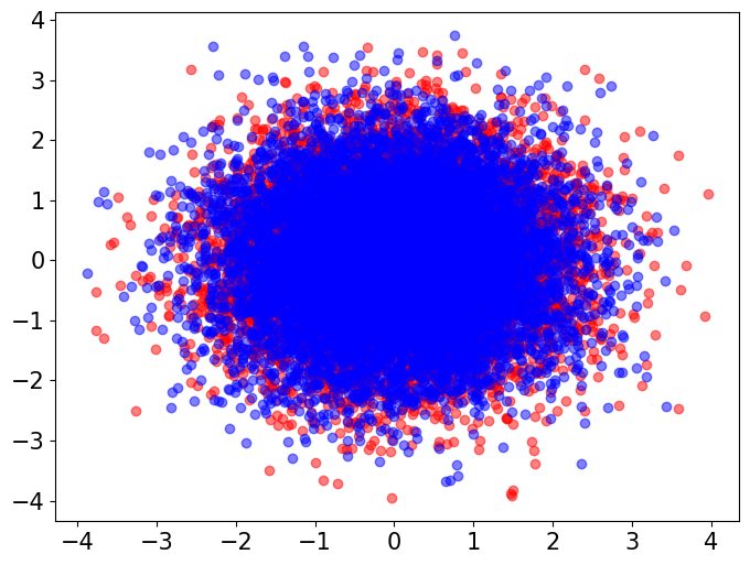
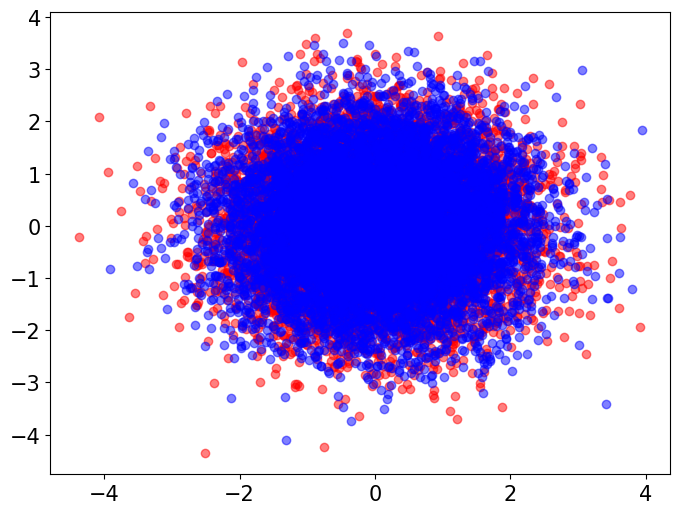
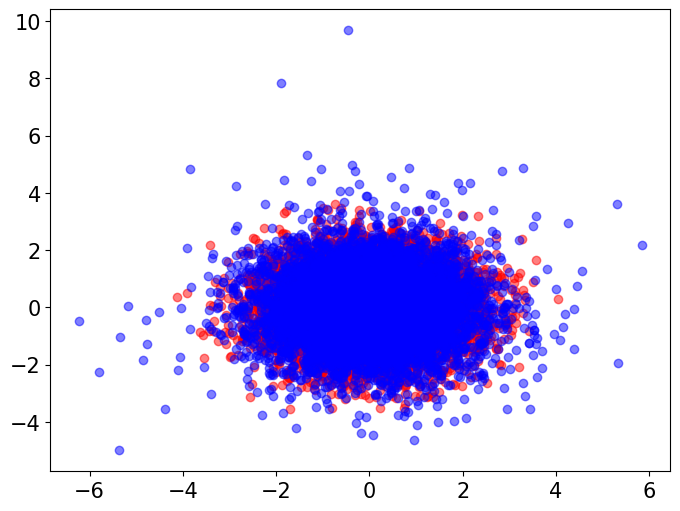
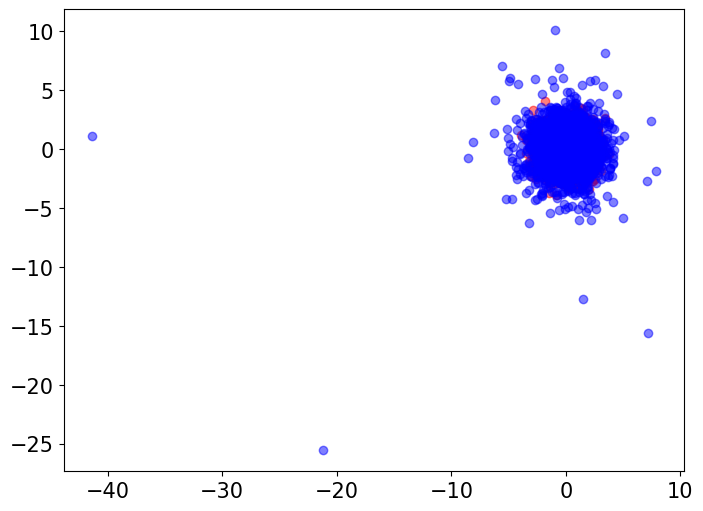
To evaluate ECS using synthetic data, we simulate random features from two classes of distributions – multivariate normal distributions and multivariate distributions. We choose the multivariate distribution because it allows us to precisely control its tail and moment behavior as we vary the degree-of-freedom parameter df. As df becomes large, the multivariate distribution has lighter tails and more higher order moments defined. On the other hand, as df becomes smaller, the distribution becomes more heavy-tailed and exhibits more outliers, with the second moment undefined when and first moment undefined when . A visualization is provided in Figure 2 in the Appendix.
We draw independent samples from a multivariate normal distribution centered at the origin with an identity covariance matrix with dimension . We then draw independent samples from five different -dimensional multivariate distributions with different degree-of-freedom parameters . These multivariate distributions are all chosen to be centered at the origin with an identity covariance matrix, which is achieved by choosing the scale matrix to be , where is the identity matrix. We then compared samples from the multivariate normal distribution with samples from each of these five multivariate distributions using ECS at and .
The above process is repeated five times. We find that, as the degree-of-freedom of the multivariate distribution decreases towards , which implies heavier tails, the value of ECS increases (Table 1). Under the normality assumptions in the FID, the population Fréchet distance yields for all five comparisons, since it only depends on the mean and covariance parameters of the distributions under comparison, which are set to be identical in the simulation. These simulations highlight the need to look beyond the first and second moments when evaluating generative models.
| ECS (T = 1) | ECS (T = 0.5) | |
| Normal versus t with df = 100 | ||
| Normal versus t with df = 10 | ||
| Normal versus t with df = 5 | ||
| Normal versus t with df = 3 | ||
| Normal versus t with df = 2.01 |
The highly controlled setting of the above simulations provides a useful heuristic for understanding the scale of ECS values. For example, the ECS value at when comparing a multivariate normal with a multivariate distribution with is around . Given the distinct higher moment and tail behavior between these two distributions, one can interpret ECS () values of as indicating a substantial mismatch between the learned and target distributions in the tails.
4.2 Empirical ECS evaluations on CIFAR10 data
We now move to show the use of ECS via the CIFAR10 (Krizhevsky, 2009) and MNIST (LeCun et al., 1998) datasets with Inception v3 embeddings. The Inception v3 neural network (Szegedy et al., 2016) is a commonly used architecture that achieves top-1 and top-5 classification error on ImageNet ILSVRC 2012, a standard benchmark that contains images from categories (Deng et al., 2009). This suggests that the last layer embeddings computed by the Inception v3 model capture relevant information about the images.
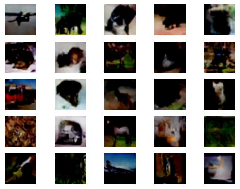
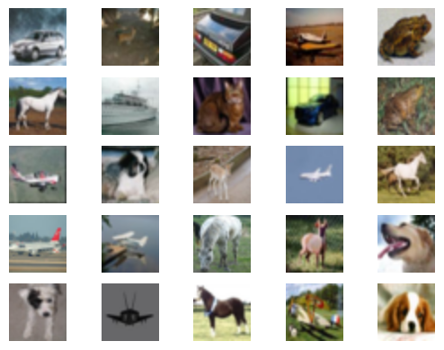
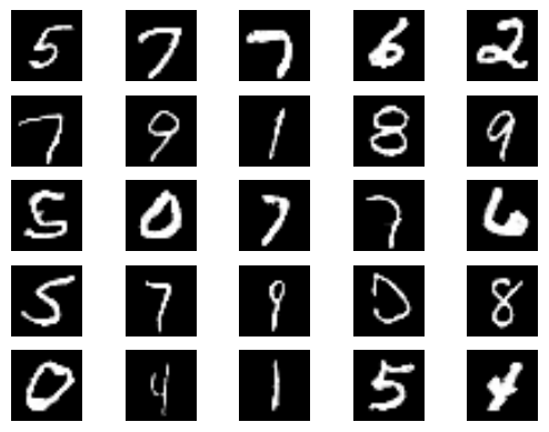
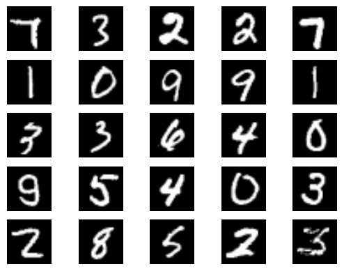
The ECS approach can work with any available embeddings. To conduct a fair comparison between FID and ECS, in our empirical study we also use Inception v3 embeddings when computing ECS. We take a Deep Convolutional Generative Adversarial Network (DC-GAN) (Radford et al., 2016) that is pretrained on CIFAR10 data. Implementation details of the DC-GAN model can be found in the Appendix. We generate synthetic images using this model. We also randomly select images from each of the CIFAR10 and MNIST testing datasets. A sample of these synthetic and real images are shown in Figure 1.
We then computed -dimensional embeddings over these real and synthetic images using the pretrained Inception v3 model that is available in PyTorch (Paszke et al., 2019; Marcel and Rodriguez, 2010). We first assess whether these embeddings collectively satisfy the normality assumption in the FID approach. We perform two statistical tests on the embeddings: the Mardia test (Mardia, 1970), which is based on kurtosis statistics, and the Henze-Zirkler test (Henze and Zirkler, 1990), which assesses normality based on the empirical characteristic function of the residuals (Table 2). These two tests present clear evidence that the Inception embeddings for both real images and synthetic images are highly non-normal across both the MNIST and CIFAR10 datasets. This suggests that the assumptions that underlie the FID are not always empirically valid, which is in line with the conclusions of prior work (Jayasumana et al., 2024).
| Mardia Kurtosis Test | Henze-Zirkler Test | |
| CIFAR10 Embeddings (Real Images) | Test Statistic p-value | Test Statistic p-value |
| CIFAR10 Embeddings (Synthetic Images) | Test Statistic p-value | Test Statistic p-value |
| MNIST Embeddings (Real Images) | Test Statistic p-value | Test Statistic p-value |
| MNIST Embeddings (Synthetic Images) | Test Statistic p-value | Test Statistic p-value |
| ECS () | ECS () | FID | FID per dimension | |
| CIFAR10 | ||||
| MNIST |
Next, using the same Inception features, we compute the FID and ECS values between the real images and synthetic images of both the MNIST and CIFAR10 datasets (Table 3). The FID values here suggests reasonable match between the synthetic and real images. It is common to see higher FID values on the CIFAR10 and MNIST datasets in the machine learning literature (Wei et al., 2022; Miyato et al., 2018; Liu et al., 2023). The ECS values here, on the other hand, suggest that the synthetic samples from the pretrained DC-GAN models do not sufficiently match the tails and higher moments of the target distribution. Taken together, the CIFAR10 and MNIST results suggest that ECS is a more accurate measure of distributional differences by avoiding the normality assumption that is violated in many real-world applications of generative deep learning methods.
5 Discussion
Deep generative models are often treated by practitioners as highly expressive (Doersch, 2016; Kingma et al., 2019) owing to the status of deep neural networks as universal function approximators (Cybenko, 1989; Barron, 1993; Hornik, 1991). Part of the folklore in the deep generative modeling literature is that, with enough training data and a large enough deep neural network, such models can generate arbitrarily accurate approximate samples from any target distribution (Hu et al., 2018). Recent work by Tam and Dunson (2025) showed that broad classes of commonly used deep generative models can only learn distributions that have light tails. This may lead to under-characterization of uncertainty when the target distribution is heavy-tailed. This simple observation seems to have evaded practitioners, in part because the metrics that are commonly used to evaluate such models ignore tail information. Developing evaluation metrics for generative models that take into account tail information can help practitioners better diagnose these problems.
In this work, we closed this evaluation gap using our embedded characteristic score (ECS) to evaluate the learned and target distributions based on higher order moments and distribution tails. We showed the behavior of ECS to better evaluate the simulated data from deep generative models versus commonly used metrics including the FID. While we focused on evaluating image generative models in this work, the approach presented here can in principle be applied to any other data modalities, as long as an appropriate data-specific embedding map is available. Developing similar evaluation metrics for more complex generative tasks, such as conditional generation and multi-modality generation, remains an open challenge; however, the ECS suggests possible approaches to these more complex tasks.
Appendix
6 Lemmas
Lemma 6.1 (Durrett (2019)).
For any real-valued random variable and any , , where is the characteristic function of . Note that while is a complex-valued function, the quantity is always real-valued.
Proof.
This inequality is due to 3.3.1 of Durrett (2019), which is proved in Theorem 3.3.17 of the same reference. ∎
7 Implementation details of empirical study
We conducted the entire empirical study in Python and PyTorch (Paszke et al., 2019). We conducted the Mardia Kurtosis test using a function implementation referenced from the open source repository https://github.com/quillan86/mvn-python. We used a function from the package Pingouin (Vallat, 2018) to perform the Henze-Zirkler test. The p values returned from these tests are too small to be represented by double precision floating points, hence we reported in Table 2 the machine epsilon value of .
Our implementation of the DC-GAN model (Radford et al., 2016) is directly referenced from the open source repository https://github.com/csinva/gan-vae-pretrained-pytorch. The pretrained weights for the DC-GAN models under both the MNIST and CIFAR10 datasets are also referenced from the same repository. The DC-GAN model architecture that is adopted in our implementation consists of 2D convolution layers in both the discriminator and generator networks.
In the empirical study, we obtained CIFAR10 (Krizhevsky, 2009) and MNIST (LeCun et al., 1998) as built-in datasets from the Torchvision package(Marcel and Rodriguez, 2010). We use the built-in pretrained Inception v3 model (Szegedy et al., 2016) from the Torchvision package to compute the Inception embeddings.
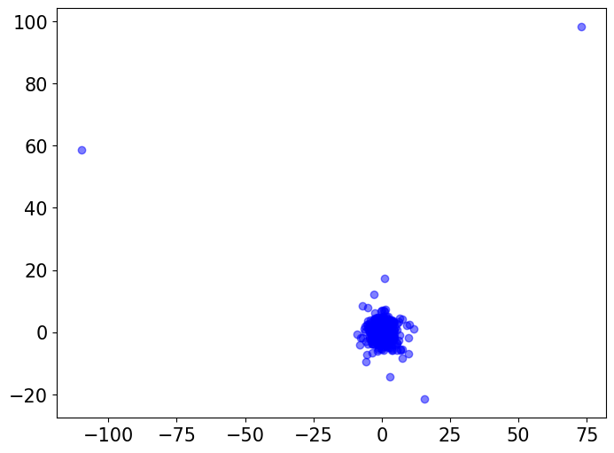
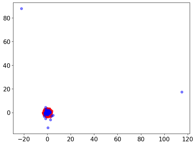
8 PCA visualization of Multivariate versus Gaussian samples
In our simulations in Section 4, we used the ECS to compare random features from a standard multivariate Gaussian distribution to random features from multivariate distributions with varying degree-of-freedom parameters . Here, we visualize the differences in tail behavior between these distributions. We draw independent random vectors with dimension from each of these distributions. We then visually compare the Gaussian vectors with each of the groups of multivariate vectors via two-dimensional PCA plots (Figure 2). We also perform a baseline Gaussian-to-Gaussian comparison by visualizing the original Gaussian samples alongside another Gaussian samples.
The visualizations indicate that, while the multivariate distribution with behaves very similarly to a Gaussian distribution, as we decrease the degree-of-freedom parameter the multivariate distribution exhibits more outliers and heavier tails, whereas the Gaussian samples exhibited no outliers.
References
- Angelopoulos et al. (2023) Angelopoulos, A. N., S. Bates, C. Fannjiang, M. I. Jordan, and T. Zrnic (2023). Prediction-powered inference. Science 382(6671), 669–674.
- Barratt and Sharma (2018) Barratt, S. and R. Sharma (2018). A note on the Inception score. arXiv preprint arXiv:1801.01973.
- Barron (1993) Barron, A. R. (1993). Universal approximation bounds for superpositions of a sigmoidal function. IEEE Transactions on Information Theory 39(3), 930–945.
- Betzalel et al. (2024) Betzalel, E., C. Penso, and E. Fetaya (2024). Evaluation metrics for generative models: An empirical study. Machine Learning and Knowledge Extraction 6(3), 1531–1544.
- Binkowski et al. (2018) Binkowski, M., D. J. Sutherland, M. Arbel, and A. Gretton (2018). Demystifying MMD GANs. In 6th International Conference on Learning Representations, ICLR 2018, Vancouver, BC, Canada, April 30 - May 3, 2018, Conference Track Proceedings. OpenReview.net.
- Chong and Forsyth (2020) Chong, M. J. and D. Forsyth (2020). Effectively unbiased FID and Inception score and where to find them. In Proceedings of the IEEE/CVF Conference on Computer Vision and Pattern Recognition, pp. 6070–6079.
- Cybenko (1989) Cybenko, G. (1989). Approximation by superpositions of a sigmoidal function. Mathematics of Control, Signals and Systems 2(4), 303–314.
- Deng et al. (2009) Deng, J., W. Dong, R. Socher, L.-J. Li, K. Li, and L. Fei-Fei (2009). ImageNet: A large-scale hierarchical image database. In 2009 IEEE Conference on Computer Vision and Pattern Recognition, pp. 248–255. IEEE.
- Denton et al. (2015) Denton, E. L., S. Chintala, R. Fergus, et al. (2015). Deep generative image models using a Laplacian pyramid of adversarial networks. Advances in Neural Information Processing Systems 28.
- Doersch (2016) Doersch, C. (2016). Tutorial on variational autoencoders. arXiv preprint arXiv:1606.05908.
- Durrett (2019) Durrett, R. (2019). Probability: Theory and Examples, Volume 49. Cambridge University Press.
- Goodfellow et al. (2014) Goodfellow, I., J. Pouget-Abadie, M. Mirza, B. Xu, D. Warde-Farley, S. Ozair, A. Courville, and Y. Bengio (2014). Generative adversarial nets. Advances in Neural Information Processing Systems 27.
- Gretton et al. (2012) Gretton, A., K. M. Borgwardt, M. J. Rasch, B. Schölkopf, and A. Smola (2012). A kernel two-sample test. The Journal of Machine Learning Research 13(1), 723–773.
- Guo et al. (2023) Guo, Z., R. Jin, C. Liu, Y. Huang, D. Shi, L. Yu, Y. Liu, J. Li, B. Xiong, D. Xiong, et al. (2023). Evaluating large language models: A comprehensive survey. arXiv preprint arXiv:2310.19736.
- Henze and Zirkler (1990) Henze, N. and B. Zirkler (1990). A class of invariant consistent tests for multivariate normality. Communications in statistics-Theory and Methods 19(10), 3595–3617.
- Heusel et al. (2017) Heusel, M., H. Ramsauer, T. Unterthiner, B. Nessler, and S. Hochreiter (2017). GANs trained by a two time-scale update rule converge to a local Nash equilibrium. Advances in Neural Information Processing Systems 30.
- Ho et al. (2020) Ho, J., A. Jain, and P. Abbeel (2020). Denoising diffusion probabilistic models. In H. Larochelle, M. Ranzato, R. Hadsell, M. Balcan, and H. Lin (Eds.), Advances in Neural Information Processing Systems 33: Annual Conference on Neural Information Processing Systems 2020, NeurIPS 2020, December 6-12, 2020, virtual.
- Hogan and Lakey (2005) Hogan, J. A. and J. D. Lakey (2005). Time-Frequency and Time-Scale Methods: Adaptive Decompositions, Uncertainty Principles, and Sampling. Springer.
- Hornik (1991) Hornik, K. (1991). Approximation capabilities of multilayer feedforward networks. Neural Networks 4(2), 251–257.
- Hu et al. (2018) Hu, T., Z. Chen, H. Sun, J. Bai, M. Ye, and G. Cheng (2018). Stein neural sampler. arXiv preprint arXiv:1810.03545.
- Jalali et al. (2024) Jalali, M., C. T. Li, and F. Farnia (2024). An information-theoretic evaluation of generative models in learning multi-modal distributions. Advances in Neural Information Processing Systems 36.
- Jayasumana et al. (2024) Jayasumana, S., S. Ramalingam, A. Veit, D. Glasner, A. Chakrabarti, and S. Kumar (2024). Rethinking fid: Towards a better evaluation metric for image generation. In Proceedings of the IEEE/CVF Conference on Computer Vision and Pattern Recognition, pp. 9307–9315.
- Jebara (2012) Jebara, T. (2012). Machine Learning: Discriminative and Generative, Volume 755. Springer Science & Business Media.
- Kingma and Welling (2014) Kingma, D. P. and M. Welling (2014). Auto-encoding variational Bayes. In Y. Bengio and Y. LeCun (Eds.), 2nd International Conference on Learning Representations, ICLR 2014, Banff, AB, Canada, April 14-16, 2014, Conference Track Proceedings.
- Kingma et al. (2019) Kingma, D. P., M. Welling, et al. (2019). An Introduction to Variational Autoencoders. Foundations and Trends® in Machine Learning 12(4), 307–392.
- Kobyzev et al. (2021) Kobyzev, I., S. J. D. Prince, and M. A. Brubaker (2021). Normalizing flows: An introduction and review of current methods. IEEE Transactions on Pattern Analysis Machine Intelligence 43(11), 3964–3979.
- Krizhevsky (2009) Krizhevsky, A. (2009). Learning multiple layers of features from tiny images.
- LeCun et al. (1998) LeCun, Y., L. Bottou, Y. Bengio, and P. Haffner (1998). Gradient-based learning applied to document recognition. Proceedings of the IEEE 86(11), 2278–2324.
- Li et al. (2017) Li, C.-L., W.-C. Chang, Y. Cheng, Y. Yang, and B. Póczos (2017). MMD GAN: Towards deeper understanding of moment matching network. Advances in Neural Information Processing Systems 30.
- Liu et al. (2023) Liu, M., J. Gan, R. Wen, T. Li, Y. Chen, and H. Chen (2023). Spiking-diffusion: Vector quantized discrete diffusion model with spiking neural networks. arXiv preprint arXiv:2308.10187.
- Lukacs (1970) Lukacs, E. (1970). Characteristic Functions. Griffin Books of Cognate Interest. Hafner Publishing Company.
- Marcel and Rodriguez (2010) Marcel, S. and Y. Rodriguez (2010). Torchvision the machine-vision package of Torch. In Proceedings of the 18th ACM International Conference on Multimedia, pp. 1485–1488.
- Mardia (1970) Mardia, K. V. (1970). Measures of multivariate skewness and kurtosis with applications. Biometrika 57(3), 519–530.
- McCaw et al. (2024) McCaw, Z. R., J. Gao, X. Lin, and J. Gronsbell (2024). Synthetic surrogates improve power for genome-wide association studies of partially missing phenotypes in population biobanks. Nature Genetics, 1–10.
- Miyato et al. (2018) Miyato, T., T. Kataoka, M. Koyama, and Y. Yoshida (2018). Spectral normalization for generative adversarial networks. arXiv preprint arXiv:1802.05957.
- Ng and Jordan (2001) Ng, A. and M. Jordan (2001). On discriminative vs. generative classifiers: A comparison of logistic regression and naive bayes. Advances in Neural Information Processing Systems 14.
- Paszke et al. (2019) Paszke, A., S. Gross, F. Massa, A. Lerer, J. Bradbury, G. Chanan, T. Killeen, Z. Lin, N. Gimelshein, L. Antiga, et al. (2019). PyTorch: An imperative style, high-performance deep learning library. Advances in Neural Information Processing Systems 32.
- Radford et al. (2016) Radford, A., L. Metz, and S. Chintala (2016). Unsupervised representation learning with deep convolutional generative adversarial networks. In Y. Bengio and Y. LeCun (Eds.), 4th International Conference on Learning Representations, ICLR 2016, San Juan, Puerto Rico, May 2-4, 2016, Conference Track Proceedings.
- Resnick (2013) Resnick, S. I. (2013). A Probability Path. Springer Science & Business Media.
- Rezende and Mohamed (2015) Rezende, D. J. and S. Mohamed (2015). Variational inference with normalizing flows. In F. R. Bach and D. M. Blei (Eds.), Proceedings of the 32nd International Conference on Machine Learning, ICML 2015, Lille, France, 6-11 July 2015, Volume 37 of JMLR Workshop and Conference Proceedings, pp. 1530–1538. JMLR.org.
- Rossler et al. (2019) Rossler, A., D. Cozzolino, L. Verdoliva, C. Riess, J. Thies, and M. Nießner (2019). Faceforensics++: Learning to detect manipulated facial images. In Proceedings of the IEEE/CVF international conference on computer vision, pp. 1–11.
- Salimans et al. (2016) Salimans, T., I. Goodfellow, W. Zaremba, V. Cheung, A. Radford, and X. Chen (2016). Improved techniques for training GANs. Advances in Neural Information Processing Systems 29.
- Song et al. (2021) Song, Y., J. Sohl-Dickstein, D. P. Kingma, A. Kumar, S. Ermon, and B. Poole (2021). Score-based generative modeling through stochastic differential equations. In 9th International Conference on Learning Representations, ICLR 2021, Virtual Event, Austria, May 3-7, 2021. OpenReview.net.
- Stein et al. (2024) Stein, G., J. Cresswell, R. Hosseinzadeh, Y. Sui, B. Ross, V. Villecroze, Z. Liu, A. L. Caterini, E. Taylor, and G. Loaiza-Ganem (2024). Exposing flaws of generative model evaluation metrics and their unfair treatment of diffusion models. Advances in Neural Information Processing Systems 36.
- Szegedy et al. (2016) Szegedy, C., V. Vanhoucke, S. Ioffe, J. Shlens, and Z. Wojna (2016). Rethinking the Inception architecture for computer vision. In Proceedings of the IEEE Conference on Computer Vision and Pattern Recognition, pp. 2818–2826.
- Tam and Dunson (2025) Tam, E. and D. Dunson (2025). On the statistical capacity of deep generative models. Technical Report.
- Theis et al. (2015) Theis, L., A. v. d. Oord, and M. Bethge (2015). A note on the evaluation of generative models. arXiv preprint arXiv:1511.01844.
- Tversky and Kahneman (1974) Tversky, A. and D. Kahneman (1974). Judgment under uncertainty: Heuristics and biases: Biases in judgments reveal some heuristics of thinking under uncertainty. Science 185(4157), 1124–1131.
- Vallat (2018) Vallat, R. (2018, November). Pingouin: statistics in Python. Journal of Open Source Software 3(31), 1026.
- Wei et al. (2022) Wei, J., M. Liu, J. Luo, A. Zhu, J. Davis, and Y. Liu (2022). DuelGAN: a duel between two discriminators stabilizes the GAN training. In European Conference on Computer Vision, pp. 290–317. Springer.
- Williams and Griffiths (2008) Williams, J. J. and T. L. Griffiths (2008). Why are people bad at detecting randomness? because it is hard. In Proceedings of the 30th Annual Conference of the Cognitive Science Society, pp. 1158–1163. Citeseer.
- Xu et al. (2018) Xu, Q., G. Huang, Y. Yuan, C. Guo, Y. Sun, F. Wu, and K. Weinberger (2018). An empirical study on evaluation metrics of generative adversarial networks. arXiv preprint arXiv:1806.07755.
- Zhou et al. (2019) Zhou, S., M. Gordon, R. Krishna, A. Narcomey, L. F. Fei-Fei, and M. Bernstein (2019). Hype: A benchmark for human eye perceptual evaluation of generative models. Advances in Neural Information Processing Systems 32.