A Domain-Agnostic Approach for Characterization of Lifelong Learning Systems
Abstract
Despite the advancement of machine learning techniques in recent years, state-of-the-art systems lack robustness to “real world” events, where the input distributions and tasks encountered by the deployed systems will not be limited to the original training context, and systems will instead need to adapt to novel distributions and tasks while deployed. This critical gap may be addressed through the development of “Lifelong Learning” systems that are capable of 1) Continuous Learning, 2) Transfer and Adaptation, and 3) Scalability. Unfortunately, efforts to improve these capabilities are typically treated as distinct areas of research that are assessed independently, without regard to the impact of each separate capability on other aspects of the system. We instead propose a holistic approach, using a suite of metrics and an evaluation framework to assess Lifelong Learning in a principled way that is agnostic to specific domains or system techniques. Through five case studies, we show that this suite of metrics can inform the development of varied and complex Lifelong Learning systems. We highlight how the proposed suite of metrics quantifies performance trade-offs present during Lifelong Learning system development - both the widely discussed Stability-Plasticity dilemma and the newly proposed relationship between Sample Efficient and Robust Learning. Further, we make recommendations for the formulation and use of metrics to guide the continuing development of Lifelong Learning systems and assess their progress in the future.
keywords:
lifelong learning , reinforcement learning , continual learning , system evaluation , catastrophic forgetting[org:apl]organization=Johns Hopkins University Applied Physics Laboratory,addressline=11100 Johns Hopkins Rd., city=Laurel, postcode=20723, state=MD, country=USA \affiliation[org:tdy]organization=Teledyne Scientific Company - Intelligent Systems Laboratory,addressline=19 T.W. Alexander Drive, city=RTP, postcode=27709, state=NC, country=USA \affiliation[org:uta]organization=Department of Computer Science, University of Texas at Austin,addressline=, city=Austin, postcode=, state=TX, country=USA \affiliation[org:usc]organization=Department of Computer Science, University of Southern California,addressline=, city=Los Angeles, postcode=, state=CA, country=USA \affiliation[org:lu]organization=Department of Computer Science, Loughborough University,addressline=, city=Loughborough, postcode=, state=England, country=UK \affiliation[org:umich]organization=Department of Electrical Engineering and Computer Science, University of Michigan,addressline=, city=Ann Arbor, postcode=, state=MI, country=USA \affiliation[org:sri]organization=SRI International,addressline=201 Washington Rd, city=Princeton, postcode=, state=NJ, country=USA \affiliation[org:utsa]organization=University of Texas at San Antonio,addressline=, city=San Antonio, postcode=, state=TX, country=USA \affiliation[org:umass]organization=Department of Computer Science, University of Massachusetts Amherst,addressline=, city=Amherst, postcode=, state=MA, country=USA \affiliation[org:snl]organization=Sandia National Laboratories,addressline=, city=Albuquerque, postcode=, state=NM, country=USA \affiliation[org:upenn]organization=Department of Computer and Information Science, University of Pennsylvania,addressline=, city=Philadelphia, postcode=, state=PA, country=USA \affiliation[org:brown]organization=Department of Computer Science, Brown University,addressline=, city=Providence, postcode=, state=RI, country=USA \affiliation[org:hrl]organization=Information and Systems Sciences Laboratory, HRL Laboratories,addressline=3011 Malibu Canyon Road, city=Malibu, postcode=90265, state=CA, country=USA \affiliation[org:vb]organization=Department of Computer Science, Vanderbilt University,addressline=, city=Nashville, postcode=, state=TN, country=USA \affiliation[org:anl]organization=Argonne National Laboratory,addressline=9700 S Cass Ave, city=Lemont, postcode=, state=IL, country=USA
1 Introduction
While machine learning (ML) has made dramatic advances in the past decade, deployment and use of data-driven ML-based systems in the real world faces a crucial challenge: the input distributions and tasks encountered by the deployed system will not be limited to the original training context, and systems will need to accommodate novel distributions and tasks while deployed. We define the challenge of Lifelong Learning (LL) as enabling a system to learn and retain knowledge of multiple tasks over its operational lifetime. Addressing this challenge requires new approaches to both algorithm development and assessment. The DARPA Lifelong Learning Machines (L2M) program was initiated in 2018 to stimulate fundamental algorithmic advances in LL and to assess these LL capabilities in complex environments. The program focused on both reinforcement learning (RL) and classification systems in diverse domains, such as CARLA (Dosovitskiy et al., 2017) (3D simulator for autonomous driving), StarCraft (Vinyals et al., 2017) (real-time strategy game), AI Habitat (Savva et al., 2019) (photorealistic 3D simulator for indoor environments), AirSim (Shah et al., 2018) (3D drone simulator), and L2Explorer (Johnson et al., 2022) (open-world exploration). The diversity of domains was motivated primarily by the research consideration of exploring LL in a broad array of contexts, and it resulted in each research team developing LL systems for their respective domains.
Throughout this work, we use the term “LL system” rather than “LL algorithm”, as the developed systems were composed of many different interacting components (e.g. regularization, experience replay, task change detection, etc.). The capability to do LL is a property of the overall system rather than any one component, and multiple metrics are needed to characterize LL systems.
The evaluation of these LL systems faced two key questions: (1) what metrics are most suitable for assessing LL, and (2) how can one apply these LL Metrics in a consistent way to different LL systems, each operating in a different domain? In particular, a primary purpose of this evaluation was to measure progress over the course of the program and to assess the strengths and weaknesses of different systems in an environment-agnostic manner, thereby providing deeper insight into LL.
The rest of this paper is organized as follows: In Section 2, we give an overview on LL systems, as well as different approaches for evaluating them. In Section 3, we introduce the core components of our approach for evaluating LL–conditions of LL, evaluation scenarios, and evaluation protocols. In Section 4, we define the metrics we use to evaluate LL systems. In Section 5, we describe a set of case studies that demonstrate the application of these metrics to varied domains. In Section 6, we conclude with insights from these case studies and give recommendations for assessing and advancing LL systems. Throughout this work, we introduce and use a number of terms which are defined in A.
2 Background
The area of machine LL has recently seen a large amount of attention in the research community (Silver et al., 2013; Chen and Liu, 2018a; Parisi et al., 2019; Hadsell et al., 2020; De Lange et al., 2021), especially through its connections to other subfields such as multi-task (Caruana, 1997; Zhang and Yang, 2021), transfer (Zhuang et al., 2019), incremental batch (Kemker et al., 2018), and online (Hoi et al., 2018) learning; as well as domain adaptation (Csurka, 2017) and generalization (Zhou et al., 2022). The distinguishing characteristic of LL is that a deployed system encounters a sequence of tasks over its lifetime, with no prior knowledge of the number, structure, duration, or re-occurrence probability of those tasks. The two key challenges are to retain expertise on previously learned tasks, thereby avoiding catastrophic forgetting (McCloskey and Cohen, 1989; Ratcliff, 1990; French, 1992, 1999; McClelland et al., 1995; Goodfellow et al., 2013), and to transfer acquired expertise to facilitate learning of new tasks (Pratt et al., 1991; Sharkey and Sharkey, 1993). Ultimately, an ideal LL system leverages relationships among tasks to improve performance across all tasks it encounters, even if the input distributions of those tasks change over a lifetime. Earlier work considered the challenges of developing algorithms to avoid forgetting and enhance transfer (Pratt, 1992; Ring, 1997).
As different methods and algorithms for LL have been developed, various approaches have been taken for evaluating these systems. A key distinction has been made between evaluation scenarios and metrics: evaluation scenarios (as shown in Figure 1) set up the structure of the lifetime of the LL system–what tasks occur, how they are presented, and how often–whereas metrics assess how well the system performed over that lifetime. We recommend Mundt et al. (2022) as a concurrently-developed work focusing on the challenges of categorizing different LL algorithms and evaluations in terms of transparency, replicability, and contextualization. When constructing a set of metrics, it is important to decide what they should be assessing. Zhu et al. (2020) frame metrics for LL as assessing either generalization (how prior knowledge facilitates initial learning on a new task) or mastery (how prior knowledge facilitates eventual performance on a new task). The suite of metrics defined in this paper extends these concepts by defining conditions of LL in Section 3.1.
2.1 Evaluation Scenarios for Different Learning Paradigms
The difficulty of quantitatively evaluating LL systems has led to a variety of approaches, both specific to the learning type and more general. Quantitatively assessing the performance of classification LL systems is often more straightforward than assessing RL systems because there are straightforward ways of generating tasks from a dataset (e.g., by splitting sets of classes into tasks, or by inducing domain shifts). However, while evaluating the LL capability of a classification system is still challenging, the evaluation scenarios used to do so tend to be specific to the classification context, such as incremental class learning, e.g., Hsu et al. (2018). Despite this, there are broader insights that are applicable for RL as well, as noted by Farquhar and Gal (2019). In particular, Hayes et al. (2018b) identify different methods of setting up the sequence of observations that constitute each lifetime of the system: sampling from different tasks in an i.i.d. fashion, grouping them by task or by class labels within a task, or (most challenging) sampling and grouping them in a non-i.i.d. fashion.
Evaluation of lifelong RL faces additional challenges: (1) RL can be highly variable within and across training runs, and across rollouts of a fixed policy (Chan et al., 2020), (2) rewards across different tasks may have different scales or extrema, or may be unbounded, and (3) it is nontrivial to design tasks with well-characterized relationships (see, e.g., Carroll and Seppi (2005)). Nonetheless, work on RL generalization and transfer offers valuable insight for LL. Kirk et al. (2021) propose a useful formalism of a “contextual Markov decision process (MDP)” where for each episode encountered by the system, the state of the MDP encodes an unseen “context” (e.g., random seeds and parameters used to specify the task). During training and test, the system encounters episodes sampled from training and test context sets respectively, with generalization assessed using zero-shot forward transfer and a “generalization gap” metric (difference in expected rewards between train and test). One of their key recommendations is to specify tasks using a combination of procedural content generation (which varies based on parameters inherent to the environment) and explicitly specified parameters. In CORA, Powers et al. (2021) present a different approach for RL performance assessment. They handcrafted benchmark tasks for four different environments (Atari (Bellemare et al., 2013), ProcGen (Cobbe et al., 2020), MiniHack (Samvelyan et al., 2021) and AI2-Thor (Kolve et al., 2017)), and proposed a standard evaluation protocol ( tasks presented sequentially, cycled times).
2.2 Metrics for Different Learning Paradigms
Metrics commonly used to assess the performance of classification LL systems include average task accuracy (ACC), forward transfer (FT) and backward transfer (BT) (also denoted FWT and BWT, respectively), as well as model size, storage and computational efficiency (Rodríguez et al., 2018; Lopez-Paz and Ranzato, 2017). Other metrics specifically developed for classification LL include Cumulative Gain, which tracks ACC after each task exposure during the course of the system’s lifetime (Prado et al., 2020), , an extension of ACC that compares the accuracy to an offline learner (Hayes et al., 2018b), and Performance Drop (Balaji et al., 2020), which uses the baseline of a multi-task model trained jointly on all tasks.
Metrics used for assessing lifelong RL include those introduced by Powers et al. (2021) for use in CORA: Forgetting (change in performance on a task before and after learning a new task) and zero-shot FT (change in performance after learning a new task, relative to a random agent). They also present baseline algorithms demonstrating the value of the metrics and tasks. Zhu et al. (2020) also propose metrics for two-task transfer learning, comparing performance with and without prior task exposure: initial performance, asymptotic performance, accumulated reward (measured by an area under the curve (AUC) calculation), and time to a threshold performance. They also propose a Transfer Ratio (asymptotic performance measured as a ratio), and performance sensitivity (variance in performance with different hyperparameter settings).
In summary, there is currently no clear guidance for defining tasks or scenarios to exercise LL, other than the guidance of having multiple tasks with some kind of structured similarity and presenting tasks to the system without specifying the order beforehand. There are also no universally accepted metrics for LL, though FT is often used for both classification and RL, and average (or cumulative) change in performance is used in RL. Overall, there is no agreed-upon standard for how to assess LL systems across different environments in a uniform manner.
2.3 DARPA L2M Program Context
The L2M program was initiated to stimulate fundamental advances in lifelong ML systems. Of particular interest were systems operating in complex and challenging environments and potentially applicable to a broad array of domains (including autonomous driving, embodied search, and real-time strategy). To this end, research conducted under the program coalesced into five different domains.
|
Environment | Domain | ||||
|---|---|---|---|---|---|---|
| SG-UPenn (5.1) |
|
|
||||
| SG-Teledyne (5.2) |
|
|
||||
| SG-HRL (5.3) |
|
|
||||
| SG-Argonne (5.4) |
|
|
||||
| SG-SRI (5.5) |
|
|
Table 1 provides information on the five LL systems that were developed as part of the program, along with their associated environments/domains. In this work, we focused on the evaluation of systems within these five environments, but the concepts and methods are broadly applicable and could work well in conjunction with a library like Avalanche (Lomonaco et al., 2021). We treated each LL system as a black box, intentionally omitting details of the constituent components. Each system was developed by a different research team and their algorithmic advances are described in publications contained in Section 5.
2.4 Evaluation of LL systems
How exactly to assess such a wide variety of LL systems operating in diverse environments was a major challenge addressed during the course of the L2M Program. We emphasize that the goal was not to identify the “best” LL system, as each environment required different learning strategies. Instead, the goal was to provide deeper insight into the strengths and weaknesses of LL systems in an environment-agnostic manner. The L2M Program test and evaluation (T&E) team and research teams collaboratively identified and defined the following key components of an LL evaluation:
-
1.
The Conditions of LL the system needed to demonstrate, which are defined in Section 3.1. These conditions specify diverse criteria identifying different components of the overall phenomena of LL.
-
2.
The Evaluation Scenarios that exercise the LL system for the purpose of computing metrics. This is an environment-agnostic template that defined the number of tasks and constraints on their relationships, as well as how they are sequenced in a given “lifetime” (or run) of the LL system. An example is demonstrated in Figure 1 and details are provided in Section 3.2.
-
3.
The overall Evaluation Protocol specifies how multiple lifetimes are set up, and consists of the Evaluation Scenarios as well as details (e.g. number of lifetimes) for obtaining statistically reliable metrics. Evaluation Protocols are discussed in Section 3.3.
-
4.
The set of LL Metrics (described in Section 4) that assess the conditions of LL. We discovered early on that a single metric would not be sufficient to cover all the conditions, and multiple metrics would be needed to characterize the LL systems.
3 Evaluation Approach
We consider three key aspects of evaluating LL systems–the conditions of LL (Section 3.1), scenarios that systems encounter (Section 3.2), and the overall protocols that specify an evaluation (Section 3.3).
3.1 Conditions of Lifelong Learning
We assert that an LL system must satisfy three necessary and sufficient conditions:
-
1.
Continuous Learning: The LL system learns a nonstationary stream of tasks (both novel and recurring), continually consolidating new information to improve performance while coping with irrelevance and noise.
-
2.
Transfer and Adaptation: As learning progresses, the LL system performs better on average on the next task it experiences, for both novel and known tasks (forward and backward transfer), maintaining performance during rapid changes in the ongoing task (adaptation).
-
3.
Scalability: The LL system continues learning for an arbitrarily long lifetime using limited resources (e.g., memory, time) in a scalable way.
These three conditions of LL have been used to drive the development of LL Metrics. They are similar to the notion of ‘generalization’ and ‘mastery’ introduced by Zhu et al. (2020), and two of our metrics can measure these concepts. The jumpstart formulation of FT (a Transfer and Adaptation metric) can be considered a measure of ‘generalization,’ and performance relative to a Single Task Expert (RP)- a Scalability metric - can be considered a measure of ‘mastery.’ It is important to point out that these conditions are partially independent; indeed, it is possible for a system to demonstrate LL in one condition but not in another. Because of this, it is all the more critical to use multiple measures to assess LL systems. The relationship between the Metrics, the Conditions of LL, and Scenario requirements associated with assessing them are discussed further in Section 4.
It is also worth noting the relationship between the above definition and related terms such as “Continual Learning” (Chen and Liu, 2018b). There are two aspects here. First, are the learning experiences from different tasks intermixed as an i.i.d sequence (online or streaming learning (Hayes et al., 2018a)) or as a non-i.i.d sequence with same-task experiences being batched together? Second, do new learning experiences expand the domain of already-learned tasks (incremental class learning), or are they entirely new tasks with new input and output domains (incremental task learning) (van de Ven and Tolias, 2018)?
Lifelong Learning, as defined above, is incremental task learning with same-task experiences batched together and with the additional constraint that the system leverage prior knowledge to become a more effective and efficient learner. The term “Continual Learning” has historically been used to loosely refer to either incremental task or class learning. However, over the past few years, it has been used more synonomously with Lifelong Learning. To avoid confusion, we consistently use the term “Lifelong Learning” in this paper.
3.2 Evaluation Scenarios
An Evaluation Scenario describes the patterns and frequency of task or task variant repetitions in sequence, and can facilitate evaluating LL systems with respect to specific metrics as well as provide insight into their strengths and weaknesses. Since certain task sequences are required to reasonably explore LL metrics, specifying a particular Scenario is a critical step in characterizing the performance of an LL system.
Two of the main scenario types used to accomplish this were Condensed and Dispersed Scenarios. Both scenario types are illustrated in Figure 2, with further details in B. Each involved a sequence of multiple tasks and variants. Individual runs had different permutation orders.
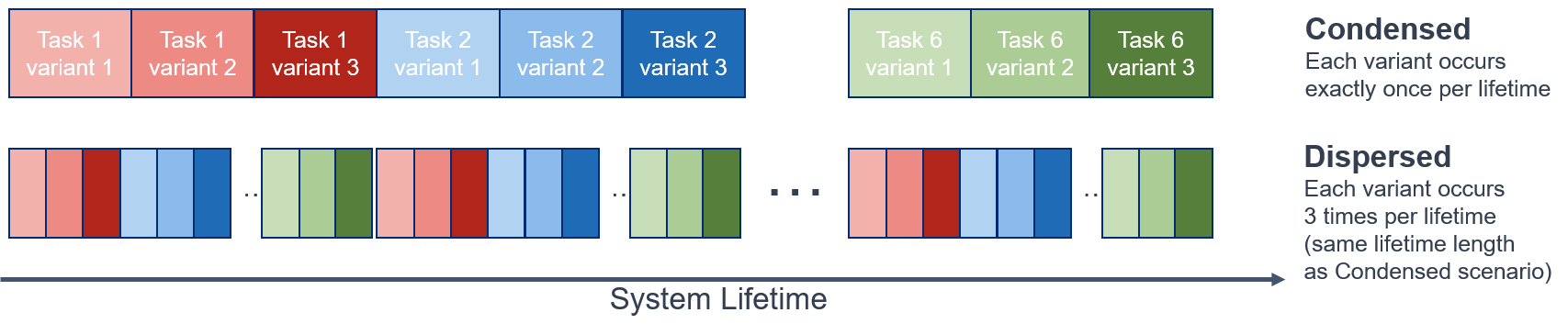
In particular, Condensed Scenarios involved concentrating all of the experience per task in one longer block. Dispersed Scenarios involved the same amount of experience per task, but with interleaved tasks in shuffled segments rather than appearing in sequence. These two scenario types were chosen to explore differences in system performance based on task ordering and appearance (since an operationalized system will not have prior knowledge of task sequences), and to ensure enough task repetitions for reasonably evaluating whether a system retained expertise on previously seen tasks. In Section 5, we see that some LL systems perform differently in various scenarios. These differences enable us to identify the characteristics, strengths, and weaknesses of an LL system.
In developing these scenario structures, we built on existing work in this area. For example, van de Ven and Tolias (2019a) proposed the class-incremental learning scenario, which is similar in structure to our condensed scenario. Concurrently to our work, Cossu et al. (2021) built off this and suggested the class-incremental with repetition scenario, which is similar to our dispersed scenario. Similarly, Stojanov et al. (2019) designs a class-incremental scenario that features parametric variation in its task design. Our framework differs in two key ways from these. First, it is meant to be more general than these scenarios, as it can accommodate LL systems that perform classification and/or reinforcement learning. Second, it incorporates task variants into its structure, which can help evaluate LL systems on environments with similar sets of tasks. Ultimately, the existence of these other scenarios is beneficial for exploring the combinatorial design space of LL scenarios, and benchmarks can be shared and extended. See B for a full example of what an Evaluation Scenario looks like.
3.3 Evaluation Protocols
In order to evaluate a particular LL system (consisting of a fixed set of hyperparameters, algorithms, and components), we recommend the use of an Evaluation Protocol. An Evaluation Protocol is a complete specification for conducting LL Scenarios to ensure reproducibility and obtain statistically reliable LL Metrics.
In addition to one or more Evaluation Scenarios, this specification consists of details about pre-deployment training (e.g., pretraining on a fixed dataset like ImageNet), and how multiple lifetimes (runs) should be generated for each scenario. This evaluation approach was used in the L2M program to foster experimentation on LL Metrics and to help researchers evaluate the performance and progress of their LL systems.
In addition to the Scenario specification, an Evaluation Protocol contains details for obtaining statistically reliable LL Metrics. As has been noted in the literature (Agarwal et al., 2021; Colas et al., 2018, 2019; Henderson et al., 2018; Dror et al., 2019), the training process for deep RL systems is noisy and variable, making it challenging to robustly evaluate them.
Our approach to generate statistically reliable LL Metrics is based on guidance in NIST/SEMATECH (2012), and similar to Colas et al. (2018). More details on this approach are provided in D. In contrast to much of the literature, which considers the problem of comparing two or more algorithms, here we focus on the challenge of obtaining reliable estimates of a system’s performance (with respect to the metrics defined in Section 4). Given such reliable estimates, we are able to determine whether a system is meeting a particular threshold. We further propose the use of LL thresholds in Section 4 to determine whether a system is demonstrating LL or not.
4 Lifelong Learning Metric Definitions
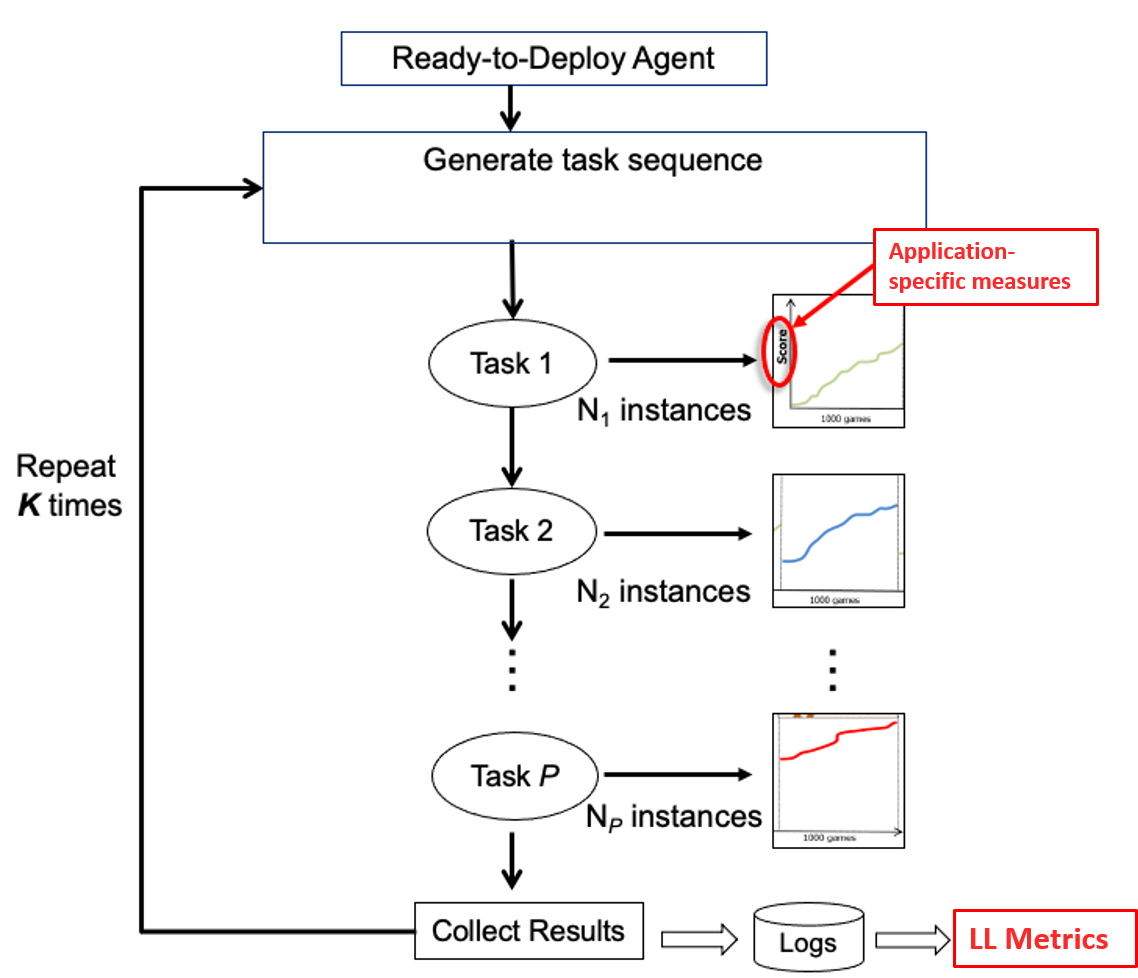
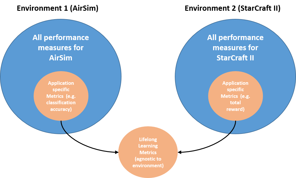
The Lifelong Learning Metrics are scenario, domain, environment and task-agnostic measures that characterize one or more Lifelong Learning (LL) capabilities across the lifetime of the system. This suite of LL Metrics, summarized in Table 2 and visualized in Figure 3, operates on application-specific performance measures (Section 4.1), making the evaluation methodology as separate as possible from the implementation details of a particular system.
| Metric Name | LL Condition | Assesses the LL system’s ability to: | ||||
|---|---|---|---|---|---|---|
|
|
Avoid catastrophic forgetting despite the introduction of new parameters or tasks | ||||
|
|
Use expertise in a known task to facilitate learning a new task | ||||
|
|
Use expertise in a new task to improve performance on a known task | ||||
|
Scalability | Match or exceed the performance of a single-task expert | ||||
|
Scalability | Make better use of learning experiences than an equivalent single-task expert |
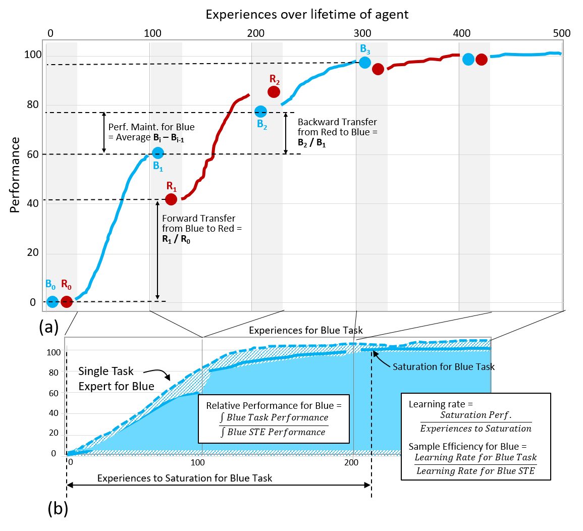
(a) White regions in the graph indicate Learning Blocks, and shaded regions indicate Evaluation Blocks. and refer to performance in the th Evaluation Block for the Blue and Red tasks, respectively. Horizontal dashed lines indicate relevant evaluation performance comparison points referred to in the example formulations of Performance Maintenance, Forward Transfer, and Backward Transfer Metrics.
(b) Single task expert (dashed blue) and LL system (solid blue) curves for the scenario shown in Fig. A. Vertical lines indicate the boundaries between each of the three Learning Blocks for the Blue Task stitched from above and overlaid with the Single task expert performance output of the same number of Learning Experiences. Experiences to Saturation and the Saturation Value for the Blue Task are also indicated on the figure to illustrate the example formulations of Sample Efficiency and Relative Performance Metrics.
The metrics are meant to work in a complementary manner in order to illustrate and characterize system capability. Thus, there is some overlap in the conditions they measure, as shown in Table 2, as well as in the means employed to do so. This approach ensures that no single metric value is responsible for fully quantifying an LL system’s performance and instead encourages deeper analysis into specific performance characteristics and the trade-offs between them.
The relationship between these metrics and the trade-offs illuminated by the case studies in Section 5 are explored further in Section 6. An in-depth discussion of the context of these metrics and their use can be found in New et al. (2022). Detailed formulations from New et al. (2022) are provided in C.2, and a publicly-available Python implementation of the metrics and a logging framework for systems that generate them are available online (Nguyen, 2022a, b).
4.1 Application-specific measures
As shown in Figure 4, an LL system performing tasks in its environment as specified by the Evaluation Protocol will generate some number of application-specific measures. Each learning experience (LX)– the minimum amount of experience with a task that enables some learning activity on the part of the system – is assumed to generate one or more scenario, domain, environment, and application-specific performance measures. A chosen subset of these application-specific measures is tracked and used to compute the LL Metrics. It is important to note that a task’s application-specific performance measures in a scenario will only be compared to the same task’s same application-specific performance measures. For example, consider an LL system that encounters two tasks and . Before encountering task , the system has a performance value for task of ; after encountering task , the system has a performance value for task of . Then, as defined in Section 4.3.2, we can assess how learning changes performance on with the backward transfer (BT) score:
There are no comparisons made between the performance values of and to compute these LL Metrics, so there is correspondingly no need to choose only one application-specific measure to assess an LL system’s performance across all tasks. In order to summarize the LL system’s performance for each Metric in a scenario, we used mean aggregation, but other options are possible.
In the following section we discuss each LL Condition, including the motivation for assessing it, the metrics associated with doing so, and the question that the metric attempts to address. At the end of each subsection, we provide LL threshold values for the metrics associated with that LL Condition.
4.2 Continuous Learning Metrics
A system demonstrating Continuous Learning will consolidate new information to improve performance while coping with irrelevance, noise, and distribution shift. The LL system needs to discover and adaptively select or ignore information that may be relevant or irrelevant. In particular, a Lifelong Learner must not be plagued by catastrophic forgetting, and performance must quickly recover when the agent is re-introduced to tasks whose performance may have degraded. While we have a metric to address whether a system has catastrophically forgotten task data, our attempt at formulating a metric to address whether a system recovers after a drop in performance was unsuccessful and is discussed more in Section 6.
4.2.1 Performance Maintenance (PM)
A Lifelong Learner should be capable of maintaining performance on each of its tasks. Performance Maintenance (PM) measures whether an LL system catastrophically forgets a previously learned task and compares a system’s performance when it first has the opportunity to learn a task to subsequent times experiencing the task. An important caveat here is that PM does not measure absolute performance levels; rather, it measures a change in performance over the course of the system’s lifetime. While there is some overlap between what PM and BT measure ( Section 4.3), BT compares a particular task’s evaluation blocks (EBs) immediately before and after learning a new task, whereas PM can be computed using any sequence of EBs, independent of how many other tasks were learned between.
4.2.2 LL threshold value for Performance Maintenance
The LL threshold value for PM is zero - this value indicates that, on average, there are no differences between initial and subsequent performances on a task. A positive value would indicate improvement over the course of a lifetime - a potential indicator of transfer. A negative value indicates forgetting. It is worth noting that this metric may be particularly sensitive to high variance in the application-specific measure ranges, since the metric computes a difference rather than use a ratio or a contrast.
| Case | Interpretation | ||
|---|---|---|---|
| PM 0 |
|
||
| PM = 0 | No forgetting; no additional learning. | ||
| PM 0 | (Does not demonstrate LL) Indicates forgetting. |
4.3 Transfer and Adaptation Metrics
One of the hallmark capabilities of a system capable of LL is the ability to leverage experience on one task toward improving performance on another. Without assuming knowledge of the details of how a system may accomplish this, we can measure progress toward this aim by computing both forward and backward transfer. At the very least, we expect that an LL system will not exhibit catastrophic forgetting, where learning a new task interferes with performance of a previously learned task.
For this particular suite of metrics, forward transfer (FT) was formulated as a jumpstart measure as introduced by Taylor and Stone (2007), where performance changes were assessed at the beginning of a learning block, measuring whether the system got a “jumpstart” on a future task. We used this formulation for FT for two primary reasons. First, the intention of these metrics was to be as domain-agnostic as possible, and addressing the nuance of how a learning curve changed could require a substantial amount of computational resources. Second, the preference was for a single value to express a system’s performance for each of the metrics, where possible. Transfer has been defined differently by others, but a jumpstart measure enables evaluation of the beginning of a system’s lifetime, which we felt was most appropriate given that we were assessing widely different systems. An important implication of this formulation to note is that for interpretability purposes, a forward transfer value is computed for only the first two tasks in a sequence.
4.3.1 Forward Transfer (FT)
FT involves a system utilizing experience from prior, seen tasks to improve on a future, unseen task. Importantly, since a primary aim in developing these metrics is their application without consideration of task specifics, we compute FT only in the first instance of each task pair as the ratio of the application-specific measure in an evaluation block before and after another task is learned. As formulated, this metric measures whether the LL system leverages data from a previously learned task to learn a new task, and it requires the presence of Evaluation Blocks before and after each new task’s first Learning Block in order to be computed. An important note about FT is that order of the tasks is important. FT may be present from Task A B, but not Task B A.
4.3.2 Backward Transfer (BT)
A system demonstrating BT will use expertise in a new task to improve performance on a known task. Unlike FT, which is only computed on the first instance of each task pair, BT can be computed for each task after every learning block (LB). This metric measures whether an LL system leverages data from a new task to improve performance on a previously learned task, and it requires EBs between each LB to measure the performance after new tasks are learned. BT is computed for each task where scenario structure allows.
4.3.3 LL Thresholds for Forward and Backward Transfer
Table 4 shows the LL threshold values for both FT and BT. A value of 1 would demonstrate no change in task performance, meaning neither forgetting nor transfer, whereas values above or below 1 would indicate transfer and interference, respectively.
| Case | Interpretation |
|---|---|
| BT / FT 1 | (Demonstrates LL) Indicates positive forward transfer. |
| BT / FT = 1 | No transfer or forgetting |
| BT / FT 1 | (Does not demonstrate LL) Indicates interference. |
4.4 Scalability Metrics
A fundamental capability for operationalized or deployable ML systems is the use of limited resources (e.g., memory, time) to accomplish or learn tasks in a scalable way. We expect an LL system to be able to sustain learning activity for arbitrarily long lifetimes including many tasks, though in practice,“arbitrarily long” and “many tasks” are relative to typical operational timescales of the application domain. While there are several ways to assess the use of limited resources, one domain-agnostic methods for doing so (used by Hayes et al. (2018b)) is to compare the performance of an LL system that is trying to learn many tasks to a single-task expert (STE) system that is learning just one task. The Sustainablity metrics assess essential components of LL because it is useful to see if an LL system is being outperformed by individual subsystems trained for each task. Scalability Metrics are an important component of system performance, in addition to being a proxy for task capacity.
4.4.1 Performance Relative to a Single Task Expert (RP)
An LL system with good performance relative to a Single Task Expert (RP) will perform well on each of its tasks when directly compared to the corresponding STE, often leveraging data from other tasks to do so. As formulated, RP measures how the performance of an LL system compares to a non LL system with comparable training. RP is related to the Transfer metrics in that a system that exhibits strong FT or BT should benefit from these effects. However, RP offers a more complete look at performance that combines all of the experience on a particular task and compares it to the performance of a STE with a similar amount of experience.
4.4.2 Sample Efficiency (SE)
Lifelong Learners are expected to sustain learning over long periods of time. The rate of performance gain of a system is a part of scalability; a system that learns quickly is efficient with the amount of experience it is exposed to. As formulated, sample efficiency (SE) describes the rate of task performance gain with additional experience. This metric measures the performance gain of the LL system by comparing the absolute level of performance (the “saturation value”) achieved by the LL system and the number of learning experiences required to get there with the corresponding STE values.
4.4.3 LL Thresholds for Relative Performance and Sample Efficiency
Determining threshold values for LL is more nuanced for the Scalability metrics. Ideally, we want the performance of an LL system to match or exceed that of an STE, as reflected in the determination of the LL thresholds in Table 5.
| Case | Interpretation |
|---|---|
| RP / SE 1 | (Demonstrates LL) Indicates Performance / Performance Gain above level of STE |
| RP / SE = 1 | Indicates Performance / Performance Gain exactly at level of STE |
| RP / SE 1 | (Does not demonstrate LL) Indicates Performance / Performance Gain below level of STE |
5 Case Studies with Lifelong Learning Systems
In this section, we examine five System Group case studies, all of which exercised the suite of LL Metrics. These metrics were computed on LL systems developed during the DARPA Lifelong Learning Machines (L2M) Program using various techniques and in different environments, as shown in Table 1. Over the course of L2M, we conducted multiple system evaluations, which are denoted by M12, M15, and M18. Each of the following subsections contains a brief overview of the corresponding LL system developed by each SG team, a description of the tasks used in each of the environments (summarized in Table 18), and a discussion of results and insights provided by the Metrics. For more details regarding the specific implementation of these systems and/or the results they generate, please see the referenced published work.
5.1 System Group UPenn - AIHabitat
5.1.1 System Overview
This section describes a case study on the development of the LL system led by SG-UPenn, a modular system that performs both classification and reinforcement learning (RL) tasks in realistic service robot settings. The core of the system, which integrates factorized models (deconvolutional factorized convolutional neural networks (DF-CNNs) for supervised learning (Lee et al., 2019) and lifelong policy gradients for faster training without forgetting (LPG-FTW) for RL (Mendez et al., 2020)), is divided into separate classification and RL pipelines, with the perception-action loop of a mobile robot. The system includes additional optional modules that can be combined with the core classification and RL pipelines, including a task-agnostic feature meta-learning module using meta Kronecker factorization optimization (Meta-KFO) (Arnold et al., 2021), intrinsic motivation via meta-learned intrinsic reward functions (Zheng et al., 2020), an alternative core RL algorithm based on the advantage actor critic (A2C) algorithm (Mnih et al., 2016), a self-supervised exploration module based on active visual mapping for robot navigation (Ramakrishnan et al., 2020), and a Markov decision process (MDP)-based curriculum learning module (Narvekar et al., 2020). These components can be turned on and off depending on the problem domain, and characterizing their effects through the set of LL Metrics proposed in this paper was a focus of the experimentation discussed in this case study. The task settings and select experimental results for the two pipelines are described below.
5.1.2 Classification Experimental Context
Classification. Lifelong classification experiments were carried out by SG-UPenn over data sets collected by simulated agents performing random walks through household environments in the AI Habitat simulator (Savva et al., 2019) using the Matterport 3D data set (Chang et al., 2017), resulting in realistic observations for household service robots derived from real world sensor data. All experiments were conducted over a fixed curriculum of object classification tasks, where each task required a mobile agent to classify a set of objects taken from an object superclass, e.g. classifying {chair, sofa, cushion, misc_seating} from the superclass seating_furniture.
5.1.3 Classification Experimental Results
| Configuration | PM | FT | BT | RP | SE |
|---|---|---|---|---|---|
| DF-CNN | |||||
| META-KFO |
This case study focuses on a specific classification experiment for which the proposed set of LL Metrics was particularly informative. The goal of this experiment was to determine the differences in performance between factorized classification models and meta-learned classification models in a lifelong supervised learning setting. To explore this, SG-UPenn ran the same set of Lifelong classification experiments over two configurations of the system: the (factorized) DF-CNN core classification pipeline and the (meta-learned) META-KFO module. The results (Table 6) show that, while both approaches show good LL performance, META-KFO provides faster learning (higher SE) whereas the DF-CNN provides more stable learning through better catastrophic forgetting mitigation (higher PM and BT, with lower standard deviations). As such, SG-UPenn prioritized future development of the DF-CNN pipeline due to the stability afforded by the factorized method.
5.1.4 Reinforcement Learning Experimental Context
Reinforcement Learning. Lifelong RL experiments were carried out in the AI Habitat simulator using the Matterport 3D data set. All experiments were conducted over a fixed curriculum of object search tasks in the form of “find a given object (e.g. a chair, a cabinet, a sink, or a plant) in a given household environment (e.g. an apartment or a town house).” The agents observed RGB images from a head-mounted camera, and their actions were direct control commands.
5.1.5 Reinforcement Learning Experimental Results
| Configuration | PM | FT | BT | RP | SE |
|---|---|---|---|---|---|
| M12 | |||||
| M15 | |||||
| M18 | 0.03 |
The first RL experiment (M12) hypothesized that intrinsic motivation would improve FT, RP, and SE in LL settings, making it an effective mechanism for knowledge reuse in lifelong RL. To test this hypothesis, SG-UPenn used the intrinsic motivation module combined with the core A2C RL algorithm. The results did not support this hypothesis, instead showing that intrinsic motivation is not an effective mechanism for lifelong learning, as shown in the M12 column of Table 7. The main issue identified was that the system was highly susceptible to catastrophic forgetting, as evidenced by the particularly low PM score. To overcome this problem, SG-UPenn focused system development on factorized methods instead, which are specifically designed to mitigate catastrophic forgetting.
The next set of RL experiments (M15) focused on evaluating the effectiveness of the factorized LPG-FTW algorithm in the realistic Habitat/Matterport environment. This system configuration used the core LPG-FTW algorithm with no additional modules. The results show significant improvement compared to the intrinsic motivation pipeline across all of the Lifelong Learning Metrics, with the exception of comparable RP. SG-UPenn notes that while the PM score was still negative, it is significantly higher than the intrinsic motivation pipeline, which shows increased mitigation of catastrophic forgetting. SG-UPenn continued to develop the LPG-FTW-based system with additional network architecture search and hyperparameter tuning that targeted the PM metric. Shown in the M18 column of Table 7, this resulted in significant improvements to both PM and FT. Contrary to the experimental results in the original LPG-FTW paper (Mendez et al., 2020), there is still relatively low performance with respect to single task experts (i.e. in the RP and SE metrics). SG-UPenn hypothesizes that this performance drop is due to the increased challenge of learning in high fidelity environments, and the higher task complexity that such environments entail.
5.2 System Group Teledyne - AirSim
5.2.1 System Overview
This section describes a case study on the development of the LL system led by SG-Teledyne. It consists of six key components, the core of which is the Uncertainty-Modulated Learning (UML) (Brna et al., 2019) algorithm. UML enables adaptation and learning in response to multiple types of uncertainty. Inspired by mechanisms of neuromodulation, UML compares its internal hypotheses against expectations and adapts its behavior based on the level of mismatch. Under high uncertainty, it re-configures itself and re-evaluates its inputs, allowing robust operation in noisy environments or in the presence of new conditions. Under low uncertainty, the algorithm can more confidently engage in long-term adaptation to learn new tasks or tune its knowledge base. Because uncertainty serves to gate learning and the type of adaptation in the system, it can prevent catastrophic forgetting and promote behaviorally-relevant adaptation. Furthermore, under very high uncertainty conditions, UML protects existing knowledge to allow one-shot learning of novel information. Finally, the algorithm can use its internal measures of uncertainty to actively seek new information to optimize learning and resource utilization (Brown et al., 2022). A limitation of UML is that it requires a robust representation of its inputs. Nonetheless, it has proven to work well when using the output layer of deep neural networks trained on datasets such as ImageNet (Deng et al., 2009) or COCO (Lin et al., 2014). Another limitation is that it learns to recognize tasks by the difference in the context of each task. Therefore, there is a requirement that each task possesses a sufficiently different context.
5.2.2 Experimental Context
The UML algorithm has been evaluated in multiple machine learning (ML) domains, including classification (Basu et al., 2017)), embodied agents (Brna et al., 2019), (Brown et al., 2022), and reinforcement learning. Under DARPA L2M, UML was evaluated using an embodied agent. Data was generated using AirSim (Shah et al., 2018) in a custom Unreal Engine 4 environment. The classification tasks were split into two “Asset Groups” loosely corresponding to notional municipal interest groups: EMA (Emergency Management) vehicles and DOT (Department of Transportation) traffic control assets (e.g., stop signs, traffic lights, etc.). Each asset group contained 2-3 individual classes of objects. The classification problems associated with each asset group formed tasks, and variants of those tasks were generated using different environmental conditions (e.g., time of day).
Experiments were conducted on permutations in ordering of these task variants, with a full evaluation across tasks being conducted after each exposure to a task.
5.2.3 Experimental Results
Table 8 shows aggregate results across all such runs generated using the SG-Teledyne system, which matched or exceeded the LL threshold value in all 5 metrics across the collected runs. These metrics enabled us to evaluate the performance of individual components in the system and their impact on LL capabilities. In an ablation experiment, Teledyne (TDY) showed that the memory consolidation technique in one of the system components (C5) was responsible for a significant gain in FT, but at the expense of PM, while other metrics remained relatively constant. These metrics enabled a deeper analysis and more complete understanding of the the impact of this component as it relates to the LL characteristics.
| Configuration | PM | FT | BT | RP | SE |
|---|---|---|---|---|---|
| TDY UML Agent | |||||
| TDY C5 Ablation |
5.3 System Group HRL - CARLA
5.3.1 System Overview
This section describes a case study on the Super Turing Evolving Lifelong Learning ARchitecture (STELLAR), the LL system developed by SG-HRL. STELLAR is a general-purpose, scalable autonomous system capable of continual online RL that is applicable to a wide range of autonomous system applications, including autonomous ground vehicles (both on-road and off-road), autonomous undersea vehicles, and autonomous aircraft, among others. It consists of a deep convolutional encoder that feeds into an actor-critic network and is trained using Proximal Policy Optimization (Schulman et al., 2017). Importantly, STELLAR integrated 11 innovative components that solve different challenges and requirements for LL. It employed Sliced Cramer Preservation (SCP) (Kolouri et al., 2020), or the sketched version of it (SCP++) (Li et al., 2021), and Complex Synapse Optimizer (Benna and Fusi, 2016) to overcome catastrophic forgetting of old tasks; Self-Preserving World Model (Ketz et al., 2019) and Context-Skill Model (Tutum et al., 2021) for backward transfer to old tasks as well as forward transfer to their variants; Neuromodulated Attention (Zou et al., 2020) for rapid performance recovery when an old task repeats; Modulated Hebbian Network (Ladosz et al., 2022) and Plastic Neuromodulated Network (Ben-Iwhiwhu et al., 2021) for rapid adaptation to new tasks; Reflexive Adaptation (Maguire et al., 2021) and Meta-Learned Instinct Network (Grbic and Risi, 2021) to safely adapt to new tasks; and Probabilistic Program Neurogenesis (Martin and Pilly, 2019) to scale up the learning of new tasks during fielded operation. More details on the precise effect of each of these components are beyond the scope of this paper; however, this case study outlines how the integrated system dynamics demonstrated LL using the proposed metrics, and how these metrics shaped the advancement of the SG-HRL system.
5.3.2 Experimental Context
STELLAR was evaluated within the CARLA driving simulator (Dosovitskiy et al., 2017) in both the Condensed and Dispersed LL Scenarios (described in Section 3.2), which were each based on three tasks with two variants per task. The agent was required to drive safely from one point to another within a designated lane (either correct or opposite) in traffic. It was given positive rewards in each time step (every 50 ms) for distance traveled towards the destination and increasing speed within the designated lane. It was given negative rewards for distance traveled away from the destination and decreasing speed within the designated lane, as well as any collision. A given episode was terminated when the destination was reached, a maximum number of time steps had elapsed, or there was any collision. SG-HRL employed two vehicle models (Audi TT [car], Kawasaki Ninja [motorcycle]) with built-in differences in physical parameters such as for the body (e.g., mass, drag coefficient) and wheels (e.g., friction, damping rate, maximum steering angle, radius). The vehicle models also differed in camera orientation (0∘ yaw for car vs. 45∘ yaw for motorcycle).
The same architecture as the STELLAR systems was used to train the STEs to saturation, thereby characterizing the ability of the STEs to learn each task. SG-HRL collected 10 STE runs per task, which were all initialized with the same “ready-to-deploy” state as the STELLAR system.
5.3.3 Experimental Results
Given that the STELLAR system integrates the 11 components listed above with the specific intent to achieve various LL capabilities, SG-HRL expected the metrics to reveal such properties of the system. Indeed in both Condensed and Dispersed scenarios, the STELLAR system exceeded the threshold for LL for 4 of the 5 metrics, with only a non-catastrophic degradation in PM of old tasks through the lifetimes (Table 9).
| Configuration | PM | FT | BT | RP | SE |
|---|---|---|---|---|---|
| Condensed (n=33) | |||||
| Dispersed (n=30) |
Further, as shown in Table 9, SG-HRL found that the performance was not significantly different between the Condensed and Dispersed scenarios. However, all the LL Metrics were numerically lower for the Dispersed scenario, with the decrements being significant at for two metrics; namely, FT ( = 0.089, Mann-Whitney U Test) and RP ( = 0.038, Mann-Whitney U Test). Potential explanations for the across-the-board numerical decrements in the metrics include: the increased cost of switching among tasks in the Dispersed scenario, greater interference from other tasks in the intervals between learning blocks for a given task, or the lack of any dependence of the strength of the consolidation mechanisms (SCP++, Self-Preserving World Model) on the performance levels acquired in the preceding learning blocks. In the Dispersed scenario, task performances in earlier learning blocks are not expected to be high due to shorter durations. In this case, strong preservation of sub-optimal task representations would interfere with subsequent learning blocks. Thus, the hyperparameters that control the degree of preservation should be reduced to improve all the LL Metrics.
| Configuration | PM | FT | BT | RP | SE |
|---|---|---|---|---|---|
| Dispersed | |||||
| Reduced SCP++ stiffness |
The STELLAR system requires considerable analysis to assess how each component contributes to various LL capabilities. This case study represents one such analysis to illustrate the impact on the metrics. SG-HRL hypothesized that stronger consolidation mechanisms would reduce LL in the Dispersed scenario which, unlike the Condensed scenario, has task repetitions. SG-HRL also predicted that strong consolidation of sub-optimal task representations after each task would negatively impact subsequent learning blocks. Data was collected for the Dispersed scenario with the SCP++ stiffness coefficient reduced to 10% of the nominal value (Table 10). As expected, SCP++ stiffness reduction resulted in improvements in 3 of the 5 metrics; namely, PM (from -2.73 to 0.26), BT by about 10%, and RP by about 30%. But the manipulation also caused decrements in the other 2 metrics; namely, FT by about 4% and SE by about 50%. Of these effects, the improvement in RP ( = 0.022, Wilcoxon Signed Rank Test) and the decrement in SE (=0.0026, Wilcoxon Signed Rank Test) were statistically significant, and the improvement in PM (=0.055, Wilcoxon Signed Rank Test) was significant at . More work will be needed to understand the dynamics of LL for task repetitions in the context of the multi-component STELLAR system. It may be the case that the degree of consolidation (structural regularization, interleaving of explicit/generative replays) should be further contingent on task learning, and SG-HRL anticipates testing this in the future.
5.4 System Group Argonne - L2Explorer
5.4.1 System Overview
This section describes a case study on the development of the LL system led by SG-Argonne. The system’s design was inspired by the brains of insects and other small animals with the motivation of developing systems capable of LL that can operate effectively at the edge (Yanguas-Gil et al., 2019).
In particular, it focuses on the use of: 1) modulatory learning and processing, which control how information is processed, as well as when and where learning takes place (Daram et al., 2020); 2) metaplasticity models, which modulate synaptic plasticity rules that keep either a memory or an internal state in order to preserve useful information (van de Ven and Tolias, 2019b); 3) broadly trained representations, which apply transfer learning to minimize what the system needs to learn during deployment, and 4) structural sparsity, which minimizes the impact of forgetting by curtailing gradient propagation in stochastic gradient descent methods (Madireddy et al., 2020).
In the context of RL, Argonne adapted these principles to propose two types of algorithms. First, they proposed a lifelong deep Q learning algorithm (Mnih et al., 2013) aimed at solving problems where a consistent policy is learned across a series of independent tasks without specific task labels. Second, they proposed a lifelong cross entropy algorithm, which applies to situations involving short, potentially contradictory tasks, where no prior information is available that would lead to accurate and consistent computations of the value of each state. For the case of deep Q learning, Argonne’s system realizes short term and long term memory buffers by implementing periodic shuffling. The size of the buffers is kept within the length of a single task.
5.4.2 Experimental Context
Over the course of the project, SG-Argonne worked in two different environments. The first and more complex environment was L2Explorer (Johnson et al., 2022), a first-person point of view environment built on top of the Unity engine (Juliani et al., 2018) that allows the creation of tasks involving open-world exploration. Argonne designed a series of tasks emphasizing different aspects of a complex policy involving target identification and selection, navigation through obstacles, navigation towards landmarks, and foraging objects while avoiding hazards. The same tasks were implemented in Roundworld, a lightweight, first-person point of view environment developed by Argonne that comprises a simpler set of objects and visual inputs, allowing us to evaluate the algorithm across two different environments.
5.4.3 Experimental Results
Table 11 shows the performance of the deep Q learning algorithms in the two different environments. In both cases there is a consistent evidence of both forward and backward transfer across tasks in the proposed scenario. One of the characteristic aspects of these environments is their task variability, both by design and driven by the open world nature of the environments. In the context of RL, this leads to large fluctuations in the values of PM and BT for both environments, with standard deviations more than one order of magnitude higher than those typically observed in image classification scenarios. On the other hand, both scenarios show values of FT, RP, and SE that are consistent with the presence of LL behaviors.
| Environment | Scenario | Agent | PM | FT | BT | RP | SE |
|---|---|---|---|---|---|---|---|
| L2Explorer | Condensed | M18 | |||||
| Roundworld | Condensed | M18 |
Having access to different metrics allows for deeper insight into variations in the system’s performance. Overall, the results obtained point to a complex picture in which the same Lifelong Learning system can exhibit different behavior depending on how well it can transfer information during its lifetime. However, further studies are needed in order to fully explore how the behavior of the agent depends on task sequence and its ability to effectively transfer relevant policies across tasks.
5.5 System Group SRI - StarCraft II
5.5.1 System Overview
This section describes a case study on the development of the LL system led by SG-SRI. The system is targeted at real-time strategy games where task change occurs naturally and throughout game play. For example, a competent Starcraft-2 (SC2) player is able to adapt their tactics to different enemy units. This section applies lifelong RL techniques to micromanagement tasks in SC2. This case study shows that the proposed metrics (a) validate that the negative effects of task drift are mitigated, (b) drive algorithm development to improve metrics, and (c) provide insights into software integration of multiple continual learners.
Components of the SG-SRI system (Sur et al., 2022; Daniels et al., 2022) include: (i) WATCH (Faber et al., 2021, 2022), a Wasserstein-based statistical changepoint detection that detects changes in the environment; (ii) Self-Taught Associative Memory (STAM) (Smith et al., 2021), to generate feature maps from RGB images in a continually updated manner; (iii) Danger detection, using the continual learner deep streaming linear discriminant analysis (DeepSLDA) (Hayes and Kanan, 2020); (iv) Compression, using the REMIND algorithm (Hayes et al., 2020) that uses Product Quantization (PQ); and (v) Sleep phase, implemented using the Eigentask framework (Raghavan et al., 2020).
5.5.2 Experimental Context
The tasks are defined using different SC2 maps called “minigames“ (Vinyals et al., 2017). The system is evaluated on the minigames of DefeatRoaches, DefeatZerglingsAndBanelings and CollectMineralShards. To each task, SG-SRI added a variant of the task that spawns two groups of enemies on each side of the map, creating a total of 3 tasks and 2 variants each. In the case of Collect, the variant has fog enabled (partial observability). SG-SRI notes that combat related tasks (Defeat) are most similar to each other (due to their reward structure) and represent 4 out of 6 tasks, so high forward transfer (jumpstart) is expected even for the single task learner.
5.5.3 Experimental Results
Table 12 shows evolution of the Eigentask algorithm driven by the proposed LL Metrics, with the current version of the system (denoted M18) achieving the criteria of lifelong learning in all but one metric (PM) in the condensed scenario and achieving the criteria of LL in several metrics for the alternating scenario. These versions, denoted as M12, M15, M18, correspond to the evaluations performed under L2M. These versions primarily differ in the generative replay architecture. The M12 model connects the autoencoders and policies one after another, whereas M15 uses a two-headed architecture using a common latent space and M18 uses hidden replay. In both scenarios, the metrics show that the M18 version that uses hidden replay is a significant improvement. Of note, the reported metrics have significantly lower variance with the M18 model compared to the M15 and M12 versions for the condensed scenario.
| Scenario | Agent | PM | FT | BT | RP | SE |
|---|---|---|---|---|---|---|
| M12 | ||||||
| Condensed | M15 | |||||
| M18 | ||||||
| M12 | ||||||
| Alternating | M15 | |||||
| M18 |
To study the effect that change detection and compression had on the overall performance of the LL system, SG-SRI performed an ablation experiment against the baseline Eigentask component in two different scenario types. PM and BT values are compared in Table 13, showing that triggering the sleep phase by statistical changepoint detection results in significantly higher PM compared to triggering it by a hand-coded schedule. This demonstrates the importance of task detection in LL systems in the task-agnostic setting and also shows that the compression of wake phase observations results in significantly higher PM. This ablation experiment demonstrates how the metrics shed insight on the impact of various system components during the development of the SG-SRI LL system.
| Agent | Performance Maintenance | Backward Transfer | ||
|---|---|---|---|---|
| Condensed | Pairwise | Condensed | Pairwise | |
| Single Task Learner (STL) | () | () | () | () |
| Eigentask (M15) | () | () | () | () |
| Eigentask + Change detection | () | () | () | () |
| Eigentask + Compression | () | () | () | () |
5.6 Summary of Case Studies of Systems Demonstrating LL
In this section we have reviewed five System Group case studies, all of which operated in different environments and employed different algorithms. Each of them used the suite of LL Metrics to inform their system development and evaluate whether their systems demonstrated the Conditions of Lifelong Learning in various experiments. In Table 14 we see that across all of the System Groups, the Lifelong Learning thresholds were met or exceeded for 52 out of 90 metrics, with Performance Maintenance only meeting the LL Threshold values in 3 of the 18 configurations compared to 13 configurations for Forward Transfer. This is unsurprising given that Performance Maintenance and Forward Transfer represent different aspects of the well-known performance trade-off between stability and plasticity, which we discuss further in Section 6.
| SG | Config | PM | FT | BT | RP | SE |
| UPenn | DF-CNN | < | < | |||
| META-KFO | < | < | < | < | ||
| RL M12 | ||||||
| RL M15 | < | |||||
| RL M18 | < | < | ||||
| Teledyne | C5 Ablated | < | ||||
| UML | < | |||||
| HRL | Condensed | < | < | |||
| Dispersed | < | < | < | |||
| SCP Ablation | < | < | ||||
| Argonne | L2Explorer | < | ||||
| Roundworld | < | |||||
| SRI | M12 Condensed | |||||
| M15 Condensed | < | < | ||||
| M18 Condensed | < | < | ||||
| M12 Alternating | ||||||
| M15 Alternating | < | |||||
| M18 Alternating |
6 Discussion
In this work, we have proposed and investigated a suite of domain- and technique- agnostic metrics to enable a systems-level development approach for evaluating Lifelong Learning systems. Such an approach is critical to supporting the multi-objective nature of Lifelong Learning (LL) system development, especially because increasingly complex solutions are required to advance the state of the art towards LL. A strength of our approach is that it simultaneously considers and quantifies varied capabilities of LL systems, rather than focusing on any single aspect of performance. By using the full suite of metrics to evaluate the System Group case studies, we were able to identify and study the performance trade-offs inherent to LL. Next, we discuss known performance trade-offs seen with these metrics, propose a new trade-off, and make recommendations for creating additional metrics for future investigations based on the accomplishments of the DARPA Lifelong Learning Machines (L2M) program.
6.1 LL Performance Trade-offs
We have argued that LL is complex and cannot be characterized by a single scalar value. This has motivated our development of a suite of metrics.
Designing an LL system must consider the following trade-offs:
-
1.
Stability vs. Plasticity: Should a system stably maintain all information it has encountered up to some point, even if that results in less flexibility to adapt to changes?
-
2.
Optimal Performance vs. Computational Cost: Should a system be optimized for maximum performance, even if that comes at a high computational cost?
-
3.
Sample Efficient vs. Robust Learning: Should a system prioritize a fast performance gain, even if it is less robust to noise or changes in the environment?
The most widely discussed trade-off in LL literature is the relationship between Stability, where a system has reliable or low-variance performance, and Plasticity, where a system is flexible and adaptable to changes (see, e.g., discussion in Mermillod et al. (2013); Grossberg (1988)). Performance Maintenance (PM) is a measure of stability, since it assesses how well a system retains task knowledge gained over the course of its lifetime; forward transfer (FT) is a measure of plasticity, as it assesses how well a system can apply knowledge from one task to another. In some cases, like the stiffness parameter experiment examined in SG-HRL’s case study (see Table 10), there is an explicit parameter that can be tuned, depending on the needs of the particular application, to prioritize reliability or flexibility. This results in somewhat expected behavior changes. In other cases, the trade-off is seen as a byproduct of targeting improvements in transfer, like in SG-Teledyne’s addition of a memory consolidation component (see Table 8), which manages the system’s stored knowledge. This addition caused marked improvement in FT– a measure of Plasticity – but at the cost of PM, a measure of Stability.
It is understood that LL systems operating in diverse environments will have varied design considerations; the availability or restriction of computational resources is one such factor. This can result in an intentional decision to choose system components that are less performant but cheaper computationally. While this discussion surfaces in the literature, particularly with regard to deployment considerations, we chose not to measure the computational resource expenditure for these evaluations. Instead, we allowed system groups to make their own assessments of progress in their domain. Even if an LL system is initially very computationally intensive, it may be possible to develop a more efficient system in the future. In non-LL, existing techniques for managing model complexity include: model distillation (Hinton et al., 2015; Gou et al., 2021), intelligently-designed model scaling strategies (Tan and Le, 2019), and investigations of broad scaling phenomena (Kaplan et al., 2020). These approaches could potentially be extended to LL; in Hayes et al. (2020), SG-SRI built on a technique called progress & compress (Schwarz et al., 2018). We see the addition of a metric to standardize the measurement of resource utilization as an excellent extension of this suite, and we summarize some initial efforts in this area in G. We collect our comments, observations and recommendations for the design and use of such a metric in Section 6.2.
We hypothesize that, as more progress is made to develop LL systems, more of these system design/performance trade-offs will be discovered. One trade-off that we observed in the SG-UPenn case study (Section 5.1) was between sample-efficient and robust learning. The system’s robustness to task or parameter changes was measured using the PM metric, and efficiency was measured via the sample efficiency (SE) metric. We can imagine a situation where a system may have an extremely robust representation of a wide range of tasks – along the lines of a subject matter expert for a particular problem space – but perhaps amassing that knowledge required significant training data and time. Conversely, a system may demonstrate aptitude for rapid mastery, but lack the broader experience to capably handle the details or nuance of edge cases.
The trade-off, then, may be that in some circumstances, optimizing for robustness comes at the cost of learning efficiency and vice versa. This goal is particularly relevant in data-poor contexts or where the cost of training is high; both of these apply in many robotic applications (like the SG-UPenn service robot setting). The LL system the SG-UPenn team built to address these challenges includes modularized components and factorized models, an approach that is well-suited to these conditions. Correspondingly, we see that when modifications were made between M15 and M18 systems to target gains in PM (Table 7), the resulting M18 results improved in PM, but at the cost of a lower Sample Efficiency. This demonstrates a consequence of the opposing aims of Robust and Sample Efficient learning. We imagine that this trade-off may not be applicable to problems with low-cost or abundant training data. However, it is apparent in this particular example, because SG-UPenn’s system design is intended for eventual transfer to service robot settings.
6.2 General Considerations for Formulation and Use of Metrics
One of the challenges of measuring LL performance is evaluating over the space of possible task sequences. Because these tasks may require orthogonal skills, it is an immense challenge to quantify a priori what ideal or even ‘good’ performance looks like for such a sequence. The standard we chose for determining thresholds for LL, which can certainly over-penalize an LL system, was perfection – perfect transfer between tasks and perfect memory of a task over the entire duration of a scenario. Over the course of the agent’s lifetime, any interference, forgetting, or performance not equal to or better than an STE was considered to be below the threshold for LL. Meeting this threshold for all lifelong learning conditions is likely to be difficult in real-world conditions. Determining an appropriate upper bound for performance on a sequence of tasks is a fundamental challenge – one that requires leveraging information like task difficulty and task similarity (and thus task transferability) – and was out of scope for this work. Below we outline some specific recommendations for metric design, some of which pose particularly unique challenges in the LL domain.
-
1.
Do not design metrics that rely on idealized performance curves
Despite knowing that we lack the ability to quantify what good performance is for a given sequence of tasks, there were some unanticipated difficulties in using the metrics related to some key assumptions about the nature and behavior of LL systems:-
(a)
Assumption 1: Learning a particular sequence of tasks is possible.
When we develop metrics to evaluate any machine learning system, we are often doing so based on an implicit assumption that a task is learnable by the system or, at least, that the system is capable of demonstrating some performance gain overthe course of its learning experiences (LXs). In the absence of baseline approaches on the same sequence of tasks to compare to, we may not even be able to say whether a sequence of tasks is learnable at all without running a cost-prohibitive number of experiments. In fact, the idea of learnability in the Lifelong Learning context has only recently been investigated in works such as Geisa et al. (2021), who explores the relationship between weak and strong learnability for both in-distribution (i.e. non-LL) and out of distribution problems. As the theory of learnability for Lifelong Learning is still developing, we must design our metrics acknowledging the potential for systems to demonstrate no learning on some tasks and, importantly, address whether or not those runs should be considered in computing the LL metrics. The results shown in Section 5 included all runs, independent of whether tasks demonstrated learning.
-
(b)
Assumption 2: In learning a sequence of tasks, performance on a previously learned task may drop, but it can and will “bounce back” when the task is shown later.
This assumption drove the design of the Performance Recovery metric, which in theory was designed to measure whether an LL system’s performance recovers after a change is introduced to its environment. To compute Performance Recovery, we first calculated the number of learning experiences the system required in order to get back to the previously attained value after a drop (recovery time), and computed the change in this number of experiences over the course of the system’s lifetime (i.e., fitted a line to the recovery times and computed the slope of the line). The idea was that a system demonstrating LL would adapt more quickly to changes as it amassed more experience.Of note, Performance Recovery could only be assessed for scenarios with many task repetitions. The use of this metric proved to be problematic, in particular because some systems would fail to “bounce back” sufficiently. This dependency of final system performance on initial LXs has been observed in the broader deep reinforcement learning (RL) space (Nikishin et al., 2022), where it was aligned with the concept of “primacy bias” from human cognition studies (Marshall and Werder, 1972). Beyond this binary challenge of a system returning to previous performance or not; given the variability in the application-specific measures, it also remained difficult to discern when performance has actually “bounced back” and to what should the new performance be compared, and how should we handle noise in these measurements? Dror et al. (2019) recommends the use of the Almost Stochastic Dominance test to mitigate the variability issue we faced, but we were unable to implement this due to the computational expense associated with this analysis.
-
(c)
Assumption 3: We can identify when a task has been “learned,” or at least, when the system performance has saturated.
Computing whether a system’s performance has saturated (and to what value) is not straightforward, in part due to the heteroskedastic nature of the learning curves. There is unpredictability to system learning, and coupling this with noisy learning makes this computation even more of a challenge. In addition, the notion of “saturation” may be ill-defined, particularly when the distribution of an environment within a learning block is nonstationary. In the case of this suite of metrics, Sample Efficiency explicitly relies on the computation of a saturation value, and Performance Maintenance compares an average of the most recent training performance to future evaluation performances – with the implicit assumption that a system has reached a stable, if not maximal, performance value at the end of a learning block.
In light of these challenges, we recommend designing an assessment – even a simple performance threshold specific to an environment – to determine whether a system has learned and to lend insight into computed metric values.
-
(a)
-
2.
Do not avoid metrics that measure overlapping concepts.
Due to some similarities in their formulation, we expected some of the metrics (e.g. PM and BT, SE and RP) to be strongly correlated. In practice, we found only weak positive correlations between those two metric pairs, as shown in Table 15. We also found that SE and PM were weakly negatively correlated, which supports our discovery of a performance trade-off between these two metrics. The strongest correlation across the metrics was between Forward Transfer and Relative Performance at = 0.45. This correlation makes sense in retrospect - a system which excels at Forward Transfer is likely to require fewer learning experiences for a task (and thus have a higher RP score) if it can benefit from another task’s learning experiences as well. Even in the case of the most correlated metrics, it was critical to have both measures since they offer an assessment of a different LL condition and add an additional perspective on assessing the whole system’s performance.
-
3.
Design metrics with clear interpretations based on the LL thresholds.
In light of the difficulty of determining an upper bound for an agent’s performance on a sequence of tasks, we made two intentional choices when formulating and interpreting the metrics. In their formulation, the LL thresholds for the metrics are clearly delineated, giving a straightforward interpretation - values above the threshold demonstrate the corresponding condition of LL, and values below do not. This was extremely useful for interpreting values and determining whether a system demonstrated lifelong learning. Though we formulated the metrics such that larger scores are better, this binary interpretation of each of the metrics allowed for a systems level analysis of performance rather than a specific focus on any one measure. -
4.
Compare performance to an STE when possible
Overall, our most robust measure of LL was the metric that baselined performance to a single task expert - Relative Performance. Relative Performance offered insight into the question of whether a system is demonstrating an improvement over previous attempts to do lifelong learning versus simply assessing whether a system demonstrates lifelong learning. This comparison to a benchmark can also be used to indicate progress over previous approaches – similar to an ablation experiment – but functions primarily as a proxy for establishing an upper bound of performance on any given task.
-
5.
Be cautious in estimating properties of data from noisy reward function distributions
As discussed in Section 3.3, Reinforcement Learning systems can be especially noisy. To remediate some issues that arise from computing values on noisy data, we preprocessed the data by smoothing it and shifting the range to exclude zero to avoid the vanishing denominator issue. In light of the noise intrinsic to these environments described by (Agarwal et al., 2021), we recommend keeping metric formulations simple. We also recommend being especially wary of second order metrics, like Performance Recovery, where noise can be compounded to the point of ineffectiveness. We hope to reformulate Performance Recovery in the future. -
6.
Be cautious about application specific metric ranges and their potential effect on ratios In initial formulations of Forward and Backward Transfer, we compared the performance before and after relevant task learning as a standard ratio under the assumption that it was unlikely for a system to achieve zero (or very small values) as an application specific measure of performance. This assumption, unfortunately, did not hold to be true. To address robustness issues that arose in those circumstances from an infinitesimal denominator, we added an alternative formulation of both forward and backward transfer using the contrast function:
where and represent a particular task performance either before or after learning a new task. While qualitatively similar to the ratio function, , contrasts differ in that they are defined when . This ensures they are well-defined in situations where application-specific measures are or approach zero; while the stability is a benefit, it can be less intuitive and therefore more complicated to interpret. Due to this difficulty in interpretation, we reported the ratio values in Section 5.
| Metric 1 | Metric 2 | Spearman Corr. | -value |
|---|---|---|---|
| Perf. Maintenance | Forward Transfer | 0.06 | 0.60 |
| Backward Transfer | 0.33 | 0.003 | |
| Relative Perf. | -0.20 | 0.07 | |
| Sample Efficiency | -0.25 | 0.03 | |
| Forward Transfer | Backward Transfer | -0.09 | 0.44 |
| Relative Perf. | 0.45 | 0.00003 | |
| Sample Efficiency | 0.01 | 0.93 | |
| Backward Transfer | Relative Perf. | -0.15 | 0.19 |
| Sample Efficiency | -0.16 | 0.14 | |
| Relative Perf. | Sample Efficiency | 0.36 | 0.001 |
7 Conclusion
In this work, we argued that evaluating advances in Lifelong Learning is a complex challenge that requires a systems approach to assessing performance and quantifying trade-offs, especially since there are currently no universally accepted metrics for Lifelong Learning. We presented the Conditions that an LL system should demonstrate as a Lifelong Learner, and developed a suite of metrics to assess those Conditions. We outlined a method for calculating the metrics in a scenario, domain, environment, and task-agnostic fashion to characterize capabilities of LL systems. We demonstrated the use of the suite of metrics via five case studies that used varied environments, illustrating the strengths and weaknesses of each system using the metrics. We discussed the quantification of three key performance trade-offs present in the development of many LL systems, and made recommendations for future metric development for LL systems.
Though the field of LL is nascent, methods and metrics for comprehensive evaluation are a critical piece in realizing a future with operationalized machine learning (ML) systems. As these LL systems increase in complexity to address current limitations, the challenge of evaluating performance and identifying strengths and weaknesses will become both more difficult and more crucial, especially in domains such as military operations or healthcare. Using a consistent suite of metrics for evaluation of complex systems in a domain- and technique-agnostic way enables a complete tracking of progress across the entire field of LL.
Many challenges remain in evaluating LL systems, including extending the computation of metrics across all lifetimes of a system, adding additional metrics to consistently quantify the computational cost trade-off, and formulating metrics that measure or account for relationships or properties of various tasks. Our suite of metrics provides a basis for extensions that can address these and other newly-discovered gaps.
8 Acknowledgements
Primary development of this work was funded by the DARPA Lifelong Learning Machines (L2M) Program. The authors would like to thank the performers in this program, particularly the members of the Definitions and Metrics Working Groups, who helped to develop and refine these LL conditions and metrics. Thanks also goes to the DARPA SETAs for this program–Conrad Bell, Robert McFarland, Rebecca McFarland, and Ben Epstein. Useful feedback on improving the manuscript was provided by Alice Jackson, Kiran Karra, Jared Markowitz, and Christopher Ratto.
9 Disclaimer
The views, opinions, and/or findings expressed are those of the author(s) and should not be interpreted as representing the official views or policies of the Department of Defense or the U.S. Government.
Appendix A Terminology
| Term | Definition |
|---|---|
| Task | Some non-trivial capability that the agent must learn, and on which performance is directly measured. A task should have parameters for stochastic and structured variation (sufficient to pose a challenging learning problem), and should have some notion of generalization. For example, in the domain of sports, “Tennis” and “Badminton” would be tasks. |
| Task Variants | Variants of a task are substantially different versions of a task - different enough to pose a significant learning challenge, and outside of the range of stochastic variation. For example, “Tennis on grass court during day” and “Tennis on clay court at night” may be considered variants. |
| Task Instance | A specific occurrence of a task that an agent encounters. In the sports domain, “Tennis” is a task, and an instance of Tennis would be a single game of tennis, on a specific kind of court, at a specific time of day and weather, with specific initial conditions, and so on. |
| Learning experience (LX) | A minimum amount of experience with a task that enables some learning activity on the part of the agent. A task instance can be a single LX, or it might consist of multiple LXs. |
| Evaluation experience (EX) | A minimum amount of experience with a task that enables some demonstration of learned activity on the part of the agent. During an EX, the LL system is being evaluated at a “frozen” state and no weight updates are allowed. |
| Block | A sequence of Experiences for a single task/variant. May be a learning block (LB) or an evaluation block (EB) |
| Lifetime | A sequence of LBs and EBs encountered by the agent once it is deployed. A lifetime starts with the agent in a “Ready-to-deploy” state. |
| Lifelong Learning Scenario | A scenario characterizes a single lifetime for an agent. It consists of a set of tasks (or task variants), any related parameterization, and optionally, specifications on how the tasks should be sequenced in the lifetime. |
| Evaluation Protocol | An evaluation protocol is a complete specification for getting statistically reliable Lifelong Learning (LL) metrics. It consists of a specification of pre-deployment training, one or more scenarios, and how multiple lifetimes (runs) are generated for each scenario. |
Appendix B Supplementary Information about Scenarios
B.1 Condensed and Dispersed Scenarios
We consider two key types of evaluation scenarios. Both consist of an interleaving sequence of learning blocks (LBs) and evaluation blocks (EBs). In the former, the Lifelong Learning (LL) system encounters learning experiences (LXs) from a specific task and improves itself. In the latter, the LL system encounters evaluation experiences (EXs) and is tested on how well it has mastered tasks. Beyond the two types here, many other variations are also devisable.
The condensed scenario assesses how well a system can retain performance on a wide variety of tasks. In it, LBs for a given task variant occur only once in the scenario, and LBs are chosen to be sufficiently long for the system to attain mastery on that block’s task.
In contrast, the dispersed scenario evaluates how well a system performs when the tasks it is exposed to change frequently. In this scenario, there are three “superblocks” (defined as a single permutation of task variants with shorter learning blocks, typically 1/3 the length of an LB in a condensed scenario). A given task variant occurs exactly once during each superblock and each superblock uses a different random permutation of task variants.
B.2 Example evaluation scenario
In Table 16, we show how tasks and task variants can be defined for two environments–SplitMNIST (Zenke et al., 2017; Shin et al., 2017; Nguyen et al., 2018), and CARLA (Dosovitskiy et al., 2017) environments, and in Table 17, we define the application-specific measures that assess LL system performance on these tasks. Our framework of LBs and EBs is sufficiently general that we can represent two diverse scenario structures (condensed and dispersed scenarios), as well as two types of learning problems–classification for SplitMNIST and reinforcement learning for CARLA. Task variants can be defined by random (e.g., random brightness perturbations for Variant-2 of SplitMNIST’s Task-1) or deterministic (e.g., fixed rotations for Variant-2 or SplitMNIST’s Task-2) transformations. In addition, experiences can be subsampled from a finite dataset (SplitMNIST) or from a more complex generator (CARLA). If desired, similar tasks can use different application-specific measures (e.g., SplitMNIST’s tasks using both average task accuracy (ACC) (Lopez-Paz and Ranzato, 2017) and (Hayes et al., 2018b)).
| SplitMNIST | CARLA | |
|---|---|---|
| Task-1 | Classify images as being either 0 or 1 1. One LX is a minibatch of sixteen images sampled from a training set 2. One EX is a minibatch of sixteen images sampled from a test set 3. Variant-1: Images are left unaltered 4. Variant-2: Images have their brightness randomly perturbed 5. Variant-3: Images have their contrasts randomly perturbed | Task-1: Navigate from one point to another 1. One LX or EX is one end-to-end navigation sequence 2. Variant-1: There is little traffic 3. Variant-2: There is heavy traffic 4. Variant-3: Navigation sequences take place at nighttime |
| Task-2 | Classify images as being either 1 or 2 1. One LX is a minibatch of sixteen images sampled from a training set 2. One EX is a minibatch of sixteen images sampled from a test set 3. Variant-1: Images are left unaltered 4. Variant-2: Images are rotated 90∘ 5. Variant-3: Images are rotated 270∘ | Follow a sedan for a specified period of time 1. One LX or EX is one end-to-end navigation sequence 2. Variant-1: It is raining during navigation sequences 3. Variant-2: The vehicle to be followed drives very quickly 4. Variant-3: The vehicle to be followed is a semi-truck |
| SplitMNIST | CARLA | |
|---|---|---|
| Application-specific measures | 1. Task-1: ACC (Lopez-Paz and Ranzato, 2017) 2. Task-2: (Hayes et al., 2018b) | 1. Task-1: Total travel time, penalized by unsafe driving 2. Task-2: Average distance to target vehicle during the navigation sequence, penalized by unsafe driving |
Appendix C Additional details on metrics
C.1 Notation for describing metrics and blocks
We introduce a compact set of notations to describe LL agent lifetimes and the quantities they output, illustrated in Figure 6.a. In general, a lifetime consists of Learning Blocks. During each learning block , the agent is exposed to experiences from a single task drawn from some larger set of possible tasks . Tasks may reoccur within a lifetime, or they may appear only once or not at all. After each Learning Block, an Evaluation Block occurs in which the agent is tested on all tasks in .
A Block consists of a sequence of (Learning or Evaluation) Experiences, and each Experience generates a single task-specific metric (e.g., a classification accuracy, reward function value, or binary outcome). These values must be preprocessed prior to calculation of LL metrics – we recommend following the procedure described in Appendix A of New et al. (2022), which is available in Nguyen (2022b).
Ultimately, each Task ’s performance in Learning Block is summarized by a sequence of values , and each Task ’s performance in the Evaluation Block after Learning Block is summarized by a scalar . Lifetimes are assumed to start with an Evaluation Block, yielding initial performance scores for all .
Baseline performance on a Task may be assessed by training a Single-Task Expert and an LL agent exposed to only one task. Relative Performance and Sample Efficiency metrics compare Learning Block performance of LL agents to STEs. We use to denote the performance in LX of the th Learning Block of an STE trained on task .
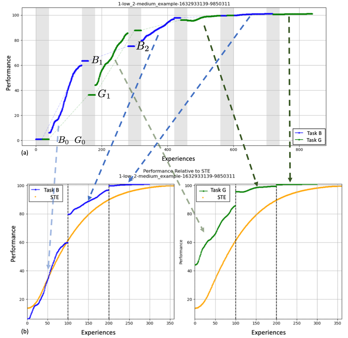
(b) Comparing the LL agent to single-task experts for the blue and green tasks (orange). Learning Blocks from the full lifetime are grouped by task and stitched together to form a task-specific learning curve.
Figure adapted from New et al. (2022).
C.2 Metric Formulations
In this section, we present pseudo-code implementations of each of the metrics described in Section 4. Our transfer metrics (Algorithm 1 and Algorithm 2) use Ratios, but Contrasts may also be used in their place (see discussion in Section 4.3 and Section 6.2).
Our algorithms for metrics that consider data from single-task experts – Relative Performance (Algorithm 3) and Sample Efficiency (Algorithm 4) – consider a simplified setting. Specifically, we assume that (1) for a given task, we have data from only a single STE, and (2) for a given task, the learning block lengths are the same across LL agents and STEs. The l2metrics package (Nguyen, 2022b) offers options for handling data when these assumptions are violated.
Appendix D Statistical Reliability
Statistical analyses can fail to recognize when two algorithms evaluated on the same benchmark are the same algorithm (Colas et al., 2018). Varying approaches have been recommended to mitigate this, including the use of the almost stochastic dominance test (Dror et al., 2019) and performance profiles during training (Agarwal et al., 2021).
In Figure 1, we present a nominal LL scenario. An agent is sent through a sequence of tasks; at the end of each lifetime, it generates a set of LL metrics. This design suggests two questions: (1) How should (the number of repetitions) be chosen ahead of time? and (2) How should metrics be aggregated across lifetimes after the fact?
Reliably assessing the variability in the responses of the agent, assuming the inherent variability of its inputs, requires assessing performance of the agent over multiple lifetimes. We outline a procedure based on guidance in NIST/SEMATECH (2012) and similar to Colas et al. (2018) to determine the number of lifetimes that need to be run, for a given Evaluation Protocol, to assess an agent’s performance.
For a given evaluation protocol, let be the random variable of values a metric can take, assumed to follow a normal distribution with population mean and standard deviation and . We seek to characterize a system’s performance by estimating . For an estimator of (typically, the sample mean of a set of values of the metric taken from multiple independent runs), we evaluate the null hypothesis that the error in estimating is no more than some error threshold . Our hypothesis of normality is strong, but it is meant to enable easy and efficient estimation of distribution properties, as well as assumptions that can be checked in practice.
One option is to choose a threshold based on the specific Protocol. However, the space of potential protocols is vast, even for a relatively small number of scenario tasks and agent configurations, and there is no guarantee that the same threshold will be informative across protocols. We follow common practice and choose the error threshold to be defined as a multiple of the standard deviation: . Thus, a procedure for determining required sample size prior to training any agents is specified by the choice of the multiple , the type I error rate , and the type II error rate . We recommend, as a default, setting , and . This yields a suggested required sample size of at least 11 runs. Evidence from works such as Agarwal et al. (2021) suggests this is likely an underestimate and so, if computational resources and time allow, more data will be of value.
With respect to the second question, we recommend two procedures for comparing the distribution of an agent’s metric values to some threshold. The student -test can be used to compare raw distributions of metrics values. However, this approach can be unreliable in the case that the values of a metric are highly non-normal (from, e.g., outliers or skewness). In that case, a more robust alternative is to binarize values by checking if they surpass that threshold and performing a statistical test on that set of binary values.
Appendix E Summary of Tasks used in SG Case Studies
| System Group | Environment | Task Descriptions |
|---|---|---|
| UPenn (Section 5.1) | AI Habitat | Classify/Find Seating Furniture |
| Classify/Find Plumbing Furniture | ||
| Classify/Find Large Furniture | ||
| Teledyne (Section 5.2) | AirSim | Classify Emergency Management Assets, low altitude |
| Drone | Classify Emergency Management Assets, high altitude | |
| Classify Dept. of Transportation Assets, low altitude | ||
| HRL (Section 5.3) | CARLA | Car navigation |
| Motorcycle navigation | ||
| Motorcycle navigation, opposite lane | ||
| ANL (Section 5.4) | L2Explorer | Identify targets |
| Navigation despite distractors | ||
| Forage specific resources | ||
| SRI (Section 5.5) | StarCraft II | Collect Resources |
| Defeat Large Enemies | ||
| Defeat Small Enemies |
Appendix F T-Test Values for SG Case Study Data
| SG | Config | PM | FT | BT | RP | SE |
| Argonne | L2Explorer | -1.31 | 8.65 | 2.93 | 1.20 | 1.20 |
| Roundworld | 5.20 | 6.93 | 2.80 | 4.08 | 16.63 | |
| HRL | Condensed | -0.23 | 12.67 | 4.00 | 6.42 | 3.67 |
| Disp | -3.77 | 18.78 | 4.10 | 6.49 | 9.06 | |
| SCP Ablation | 0.25 | 10.75 | 3.45 | 9.10 | 5.87 | |
| SRI | M12 Condensed | -5.13 | 8.31 | -0.12 | -2.36 | 6.77 |
| M15 Condensed | -5.52 | 8.31 | 2.46 | 4.57 | 15.31 | |
| M18 Condensed | -6.73 | 15.31 | 0.62 | 5.72 | 10.95 | |
| M12 Alternating | -4.66 | 1.05 | -3.53 | -5.57 | 6.15 | |
| M15 Alternating | -5.44 | 1.15 | -5.09 | -4.84 | 8.51 | |
| M18 Alternating | -2.91 | 2.13 | -2.31 | -2.52 | 5.09 | |
| Teledyne | C5 Ablated | 1.98 | 79.33 | 0.72 | 2.71 | 3.55 |
| UML | 2.82 | 72.01 | 3.15 | 1.80 | 3.13 | |
| UPenn | DF-CNN | -2.36 | 0.63 | -2.24 | 22.00 | 29.41 |
| META-KFO | -8.20 | NaN | -7.99 | 20.83 | 31.47 | |
| RL M12 | -5.59 | -0.28 | 0.26 | -7.14 | -2.52 | |
| RL M15 | -2.37 | 3.39 | 4.11 | -14.43 | 1.56 | |
| RL M18 | 0.99 | 2.97 | 5.21 | -13.27 | -18.79 |
Appendix G Computational Costs of Lifelong Learning
Different LL algorithms can potentially have different computational costs. For example, an algorithm with experience replay might be more computationally expensive during deployment than one that grew the network as needed. Unfortunately, it is challenging to compare these costs across agents given differences in learning frameworks, distributed training, and environments. Instead, we attempted to get insight into , the relative cost imposed by an LL system as it tries to preserve and transfer learning across multiple tasks, compared to the same algorithm being applied to just a single task (see Table 20). For instance, indicates that it takes 1.5x more computational effort to process a single learning experience (LX) during deployment (when learning multiple tasks) compared to a single-task setting.
| Elapsed time for a single lifetime with multiple tasks, averaged across the submitted runs. | |
|---|---|
| Elapsed time for the single task expert, trained to saturation. | |
| Time Cost per LX, for the multi-task lifelong learner | |
| Time Cost per LX for the single-task expert | |
| Cost overhead of lifelong learning |
It should be noted that is a crude measure, with several limitations: it does not distinguish between learning and evaluation experiences, does not take overall performance into account, and does not separately consider agent and environment computation (for example, a complex 3D environment like AirSim may take more computational resources to render than StarCraft). Even so, can provide useful insight. When applied to preliminary versions of the LL algorithms developed by the SGs, the s ranged from 1.27 to 2.53, indicating that some LL algorithms potentially had twice the multi-task overhead of others. Notably, the s are contained within a small band of values, which is remarkable given the diversity of environments, tasks and learning algorithms.
References
- Agarwal et al. (2021) Agarwal, R., Schwarzer, M., Castro, P.S., Courville, A., Bellemare, M.G., 2021. Deep reinforcement learning at the edge of the statistical precipice, in: Thirty-Fifth Conference on Neural Information Processing Systems.
- Arnold et al. (2021) Arnold, S., Iqbal, S., Sha, F., 2021. When MAML can adapt fast and how to assist when it cannot, in: International Conference on Artificial Intelligence and Statistics, PMLR. pp. 244–252.
- Balaji et al. (2020) Balaji, Y., Farajtabar, M., Yin, D., Mott, A., Li, A., 2020. The effectiveness of memory replay in large scale continual learning. arXiv preprint arXiv:2010.02418 .
- Basu et al. (2017) Basu, S., Karki, M., Ganguly, S., DiBiano, R., Mukhopadhyay, S., Gayaka, S., Kannan, R., Nemani, R., 2017. Learning sparse feature representations using probabilistic quadtrees and deep belief nets. Neural Processing Letters 45, 855–867.
- Bellemare et al. (2013) Bellemare, M.G., Naddaf, Y., Veness, J., Bowling, M., 2013. The Arcade learning environment: An evaluation platform for general agents. Journal of Artificial Intelligence Research 47, 253–279.
- Ben-Iwhiwhu et al. (2021) Ben-Iwhiwhu, Dick, Ketz, Pilly, Soltoggio, 2021. Context meta-reinforcement learning via neuromodulation. CoRR abs/2111.00134. URL: http://arxiv.org/abs/2111.00134, arXiv:2111.00134.
- Benna and Fusi (2016) Benna, Fusi, 2016. Computational principles of synaptic memory consolidation. Nature Neuroscience 19, 1697–1706. URL: https://github.com/GMvandeVen/complex-synapses.
- Brna et al. (2019) Brna, A.P., Brown, R.C., Connolly, P.M., Simons, S.B., Shimizu, R.E., Aguilar-Simon, M., 2019. Uncertainty-based modulation for lifelong learning. Neural Networks 120, 129–142. URL: https://www.sciencedirect.com/science/article/pii/S0893608019302722, doi:https://doi.org/10.1016/j.neunet.2019.09.011. special Issue in Honor of the 80th Birthday of Stephen Grossberg.
- Brown et al. (2022) Brown, R., Brna, A., Cook, J., Park, S., Aguilar-Simon, M., 2022. Uncertainty-driven control for a self-supervised lifelong learning drone, in: International Geoscience and Remote Sensing Symposium, IEEE, Kuala Lumpur, Malaysia.
- Carroll and Seppi (2005) Carroll, J., Seppi, K., 2005. Task similarity measures for transfer in reinforcement learning task libraries, in: Proceedings. 2005 IEEE International Joint Conference on Neural Networks, 2005., pp. 803–808 vol. 2. doi:10.1109/IJCNN.2005.1555955.
- Caruana (1997) Caruana, R., 1997. Multitask learning. Machine Learning 28, 41–75. URL: https://doi.org/10.1023/A:1007379606734, doi:10.1023/A:1007379606734.
- Chan et al. (2020) Chan, S.C., Fishman, S., Korattikara, A., Canny, J., Guadarrama, S., 2020. Measuring the reliability of reinforcement learning algorithms, in: International Conference on Learning Representations. URL: https://openreview.net/forum?id=SJlpYJBKvH.
- Chang et al. (2017) Chang, A., Dai, A., Funkhouser, T., Halber, M., Niessner, M., Savva, M., Song, S., Zeng, A., Zhang, Y., 2017. Matterport3D: Learning from RGB-D data in indoor environments. International Conference on 3D Vision (3DV) .
- Chen and Liu (2018a) Chen, Z., Liu, B., 2018a. Lifelong machine learning. Morgan & Claypool Publishers.
- Chen and Liu (2018b) Chen, Z., Liu, B., 2018b. Lifelong Machine Learning, Second Edition. volume 12. URL: https://www.morganclaypool.com/doi/10.2200/S00832ED1V01Y201802AIM037.
- Cobbe et al. (2020) Cobbe, K., Hesse, C., Hilton, J., Schulman, J., 2020. Leveraging procedural generation to benchmark reinforcement learning, in: III, H.D., Singh, A. (Eds.), Proceedings of the 37th International Conference on Machine Learning, PMLR. pp. 2048–2056. URL: https://proceedings.mlr.press/v119/cobbe20a.html.
- Colas et al. (2018) Colas, C., Sigaud, O., Oudeyer, P., 2018. How many random seeds? Statistical power analysis in deep reinforcement learning experiments. CoRR abs/1806.08295. URL: http://arxiv.org/abs/1806.08295, arXiv:1806.08295.
- Colas et al. (2019) Colas, C., Sigaud, O., Oudeyer, P.Y., 2019. A hitchhiker’s guide to statistical comparisons of reinforcement learning algorithms. arXiv:1904.06979.
- Cossu et al. (2021) Cossu, A., Graffieti, G., Pellegrini, L., Maltoni, D., Bacciu, D., Carta, A., Lomonaco, V., 2021. Is class-incremental enough for continual learning? URL: https://arxiv.org/abs/2112.02925, doi:10.48550/ARXIV.2112.02925.
- Csurka (2017) Csurka, G., 2017. Domain Adaptation in Computer Vision Applications. 1st ed., Springer Publishing Company, Incorporated.
- Daniels et al. (2022) Daniels, Z., Raghavan, A., Hostetler, J., Rahman, A., Sur, I., Piacentino, M., Divakaran, A., 2022. Model-free generative replay for lifelong reinforcement learning: Application to starcraft-2, in: Conference on Lifelong Learning Agents, Proceedings of Machine Learning Research.
- Daram et al. (2020) Daram, A., Yanguas-Gil, A., Kudithipudi, D., 2020. Exploring neuromodulation for dynamic learning. Frontiers in Neuroscience 14. URL: https://www.frontiersin.org/article/10.3389/fnins.2020.00928, doi:10.3389/fnins.2020.00928.
- De Lange et al. (2021) De Lange, M., Aljundi, R., Masana, M., Parisot, S., Jia, X., Leonardis, A., Slabaugh, G., Tuytelaars, T., 2021. A continual learning survey: Defying forgetting in classification tasks. IEEE Transactions on Pattern Analysis and Machine Intelligence .
- Deng et al. (2009) Deng, J., Dong, W., Socher, R., Li, L.J., Li, K., Fei-Fei, L., 2009. ImageNet: A large-scale hierarchical image database, in: 2009 IEEE Conference on Computer Vision and Pattern Recognition, pp. 248–255. doi:10.1109/CVPR.2009.5206848.
- Dosovitskiy et al. (2017) Dosovitskiy, A., Ros, G., Codevilla, F., Lopez, A., Koltun, V., 2017. CARLA: An open urban driving simulator, in: Proceedings of the 1st Annual Conference on Robot Learning, pp. 1–16.
- Dror et al. (2019) Dror, R., Shlomov, S., Reichart, R., 2019. Deep dominance - how to properly compare deep neural models, in: Proceedings of the 57th Annual Meeting of the Association for Computational Linguistics, Association for Computational Linguistics, Florence, Italy. pp. 2773–2785. URL: https://aclanthology.org/P19-1266, doi:10.18653/v1/P19-1266.
- Faber et al. (2021) Faber, K., Corizzo, R., Sniezynski, B., Baron, M., Japkowicz, N., 2021. Watch: Wasserstein change point detection for high-dimensional time series data, in: 2021 IEEE International Conference on Big Data (Big Data), IEEE. pp. 4450–4459.
- Faber et al. (2022) Faber, K., Corizzo, R., Sniezynski, B., Baron, M., Japkowicz, N., 2022. Lifewatch: Lifelong wasserstein change point detection, in: 2022 International Joint Conference on Neural Networks (IJCNN), IEEE.
- Farquhar and Gal (2019) Farquhar, S., Gal, Y., 2019. Towards robust evaluations of continual learning. arXiv:1805.09733.
- French (1992) French, R.M., 1992. Semi-distributed representations and catastrophic forgetting in connectionist networks. Connection Science 4, 365–377. URL: https://doi.org/10.1080/09540099208946624, doi:10.1080/09540099208946624, arXiv:https://doi.org/10.1080/09540099208946624.
- French (1999) French, R.M., 1999. Catastrophic forgetting in connectionist networks. Trends in Cognitive Sciences 3, 128–135. URL: https://www.sciencedirect.com/science/article/pii/S1364661399012942, doi:https://doi.org/10.1016/S1364-6613(99)01294-2.
- Geisa et al. (2021) Geisa, A., Mehta, R., Helm, H.S., Dey, J., Eaton, E., Dick, J., Priebe, C.E., Vogelstein, J.T., 2021. Towards a theory of out-of-distribution learning. URL: https://arxiv.org/abs/2109.14501, doi:10.48550/ARXIV.2109.14501.
- Goodfellow et al. (2013) Goodfellow, I.J., Mirza, M., Xiao, D., Courville, A., Bengio, Y., 2013. An empirical investigation of catastrophic forgetting in gradient-based neural networks. URL: https://arxiv.org/abs/1312.6211, doi:10.48550/ARXIV.1312.6211.
- Gou et al. (2021) Gou, J., Yu, B., Maybank, S.J., Tao, D., 2021. Knowledge distillation: A survey. International Journal of Computer Vision 129, 1789–1819. URL: https://doi.org/10.1007%2Fs11263-021-01453-z, doi:10.1007/s11263-021-01453-z.
- Grbic and Risi (2021) Grbic, Risi, 2021. Safer reinforcement learning through transferable instinct networks. Proceedings of the 2021 Conference on Artificial Life .
- Grossberg (1988) Grossberg, S., 1988. How Does the Brain Build a Cognitive Code?. MIT Press, Cambridge, MA, USA. p. 347–399.
- Hadsell et al. (2020) Hadsell, R., Rao, D., Rusu, A.A., Pascanu, R., 2020. Embracing change: Continual learning in deep neural networks. Trends in Cognitive Sciences 24, 1028–1040. URL: https://doi.org/10.1016/j.tics.2020.09.004, doi:10.1016/j.tics.2020.09.004.
- Hayes et al. (2018a) Hayes, T.L., Cahill, N.D., Kanan, C., 2018a. Memory efficient experience replay for streaming learning. arXiv:1809.05922 [cs, stat] URL: http://arxiv.org/abs/1809.05922. arXiv: 1809.05922.
- Hayes et al. (2020) Hayes, T.L., Kafle, K., Shrestha, R., Acharya, M., Kanan, C., 2020. Remind your neural network to prevent catastrophic forgetting, in: European Conference on Computer Vision, Springer. pp. 466–483.
- Hayes and Kanan (2020) Hayes, T.L., Kanan, C., 2020. Lifelong machine learning with deep streaming linear discriminant analysis, in: Proceedings of the IEEE/CVF Conference on Computer Vision and Pattern Recognition Workshops, pp. 220–221.
- Hayes et al. (2018b) Hayes, T.L., Kemker, R., Cahill, N.D., Kanan, C., 2018b. New metrics and experimental paradigms for continual learning, in: 2018 IEEE/CVF Conference on Computer Vision and Pattern Recognition Workshops (CVPRW), pp. 2112–21123. doi:10.1109/CVPRW.2018.00273.
- Henderson et al. (2018) Henderson, P., Islam, R., Bachman, P., Pineau, J., Precup, D., Meger, D., 2018. Deep reinforcement learning that matters, in: Proceedings of the Thirty-Second AAAI Conference on Artificial Intelligence and Thirtieth Innovative Applications of Artificial Intelligence Conference and Eighth AAAI Symposium on Educational Advances in Artificial Intelligence, AAAI Press.
- Hinton et al. (2015) Hinton, G., Vinyals, O., Dean, J., 2015. Distilling the knowledge in a neural network. URL: https://arxiv.org/abs/1503.02531, doi:10.48550/ARXIV.1503.02531.
- Hoi et al. (2018) Hoi, S.C.H., Sahoo, D., Lu, J., Zhao, P., 2018. Online learning: A comprehensive survey. CoRR abs/1802.02871. URL: http://arxiv.org/abs/1802.02871, arXiv:1802.02871.
- Hsu et al. (2018) Hsu, Y., Liu, Y., Kira, Z., 2018. Re-evaluating continual learning scenarios: A categorization and case for strong baselines. CoRR abs/1810.12488. URL: http://arxiv.org/abs/1810.12488, arXiv:1810.12488.
- Johnson et al. (2022) Johnson, E.C., Nguyen, E.Q., Schreurs, B., Ewulum, C.S., Ashcraft, C., Fendley, N.M., Baker, M.M., New, A., Vallabha, G.K., 2022. L2Explorer: A lifelong reinforcement learning assessment environment. URL: https://arxiv.org/abs/2203.07454, doi:10.48550/ARXIV.2203.07454.
- Juliani et al. (2018) Juliani, A., Berges, V.P., Teng, E., Cohen, A., Harper, J., Elion, C., Goy, C., Gao, Y., Henry, H., Mattar, M., Lange, D., 2018. Unity: A general platform for intelligent agents. URL: https://arxiv.org/abs/1809.02627, doi:10.48550/ARXIV.1809.02627.
- Kaplan et al. (2020) Kaplan, J., McCandlish, S., Henighan, T., Brown, T.B., Chess, B., Child, R., Gray, S., Radford, A., Wu, J., Amodei, D., 2020. Scaling laws for neural language models. URL: https://arxiv.org/abs/2001.08361, doi:10.48550/ARXIV.2001.08361.
- Kemker et al. (2018) Kemker, R., McClure, M., Abitino, A., Hayes, T.L., Kanan, C., 2018. Measuring catastrophic forgetting in neural networks, in: Proceedings of the Thirty-Second AAAI Conference on Artificial Intelligence and Thirtieth Innovative Applications of Artificial Intelligence Conference and Eighth AAAI Symposium on Educational Advances in Artificial Intelligence, AAAI Press.
- Ketz et al. (2019) Ketz, N., Kolouri, S., Pilly, P.K., 2019. Continual learning using world models for pseudo-rehearsal. CoRR abs/1903.02647. URL: http://arxiv.org/abs/1903.02647, arXiv:1903.02647.
- Kirk et al. (2021) Kirk, R., Zhang, A., Grefenstette, E., Rocktäschel, T., 2021. A survey of generalisation in deep reinforcement learning. CoRR abs/2111.09794. URL: https://arxiv.org/abs/2111.09794, arXiv:2111.09794.
- Kolouri et al. (2020) Kolouri, S., Ketz, N.A., Soltoggio, A., Pilly, P.K., 2020. Sliced Cramer synaptic consolidation for preserving deeply learned representations, in: International Conference on Learning Representations.
- Kolve et al. (2017) Kolve, E., Mottaghi, R., Han, W., VanderBilt, E., Weihs, L., Herrasti, A., Gordon, D., Zhu, Y., Gupta, A., Farhadi, A., 2017. AI2-THOR: An interactive 3D environment for visual AI. URL: https://arxiv.org/abs/1712.05474, doi:10.48550/ARXIV.1712.05474.
- Ladosz et al. (2022) Ladosz, P., Ben-Iwhiwhu, E., Dick, J., Ketz, N., Kolouri, S., Krichmar, J.L., Pilly, P.K., Soltoggio, A., 2022. Deep reinforcement learning with modulated Hebbian plus Q-network architecture. IEEE Transactions on Neural Networks and Learning Systems 33, 2045–2056. doi:10.1109/TNNLS.2021.3110281.
- Lee et al. (2019) Lee, S., Stokes, J., Eaton, E., 2019. Learning shared knowledge for deep lifelong learning using deconvolutional networks., in: IJCAI, pp. 2837–2844.
- Li et al. (2021) Li, Krishnan, Wu, Kolouri, Pilly, Braverman, 2021. Lifelong learning with sketched structural regularization. Proceedings of the 2021 Asian Conference on Machine Learning .
- Lin et al. (2014) Lin, T.Y., Maire, M., Belongie, S., Bourdev, L., Girshick, R., Hays, J., Perona, P., Ramanan, D., Zitnick, C.L., Dollár, P., 2014. Microsoft COCO: Common objects in context. URL: https://arxiv.org/abs/1405.0312, doi:10.48550/ARXIV.1405.0312.
- Lomonaco et al. (2021) Lomonaco, V., Pellegrini, L., Cossu, A., Carta, A., Graffieti, G., Hayes, T.L., Lange, M.D., Masana, M., Pomponi, J., van de Ven, G.M., Mundt, M., She, Q., Cooper, K., Forest, J., Belouadah, E., Calderara, S., Parisi, G.I., Cuzzolin, F., Tolias, A.S., Scardapane, S., Antiga, L., Amhad, S., Popescu, A., Kanan, C., van de Weijer, J., Tuytelaars, T., Bacciu, D., Maltoni, D., 2021. Avalanche: an end-to-end library for continual learning. CoRR abs/2104.00405. URL: https://arxiv.org/abs/2104.00405, arXiv:2104.00405.
- Lopez-Paz and Ranzato (2017) Lopez-Paz, D., Ranzato, M., 2017. Gradient episodic memory for continual learning. Advances in neural information processing systems 30.
- Madireddy et al. (2020) Madireddy, S., Yanguas-Gil, A., Balaprakash, P., 2020. Neuromodulated neural architectures with local error signals for memory-constrained online continual learning. URL: https://arxiv.org/abs/2007.08159, doi:10.48550/ARXIV.2007.08159.
- Maguire et al. (2021) Maguire, Ketz, Pilly, Mouret, 2021. An online data-driven emergency-reponse method for autonomous agents in unforeseen situations. CoRR abs/2112.09670. URL: http://arxiv.org/abs/2112.09670, arXiv:2112.09670.
- Marshall and Werder (1972) Marshall, P.H., Werder, P.R., 1972. The effects of the elimination of rehearsal on primacy and recency. Journal of Verbal Learning and Verbal Behavior 11, 649–653. URL: https://www.sciencedirect.com/science/article/pii/S0022537172800495, doi:https://doi.org/10.1016/S0022-5371(72)80049-5.
- Martin and Pilly (2019) Martin, Pilly, 2019. Probabilistic program neurogenesis. Proceedings of the 2019 Conference on Artificial Life .
- McClelland et al. (1995) McClelland, J.L., McNaughton, B.L., O’Reilly, R.C., 1995. Why there are complementary learning systems in the hippocampus and neocortex: insights from the successes and failures of connectionist models of learning and memory. Psychological review 102, 419.
- McCloskey and Cohen (1989) McCloskey, M., Cohen, N.J., 1989. Catastrophic interference in connectionist networks: The sequential learning problem, Academic Press. volume 24 of Psychology of Learning and Motivation, pp. 109–165. URL: https://www.sciencedirect.com/science/article/pii/S0079742108605368, doi:https://doi.org/10.1016/S0079-7421(08)60536-8.
- Mendez et al. (2020) Mendez, J.A., Wang, B., Eaton, E., 2020. Lifelong policy gradient learning of factored policies for faster training without forgetting. CoRR abs/2007.07011. URL: https://arxiv.org/abs/2007.07011, arXiv:2007.07011.
- Mermillod et al. (2013) Mermillod, M., Bugaiska, A., Bonin, P., 2013. The stability-plasticity dilemma: investigating the continuum from catastrophic forgetting to age-limited learning effects. Frontiers in Psychology 4. URL: https://www.frontiersin.org/article/10.3389/fpsyg.2013.00504, doi:10.3389/fpsyg.2013.00504.
- Mnih et al. (2016) Mnih, V., Badia, A.P., Mirza, M., Graves, A., Lillicrap, T., Harley, T., Silver, D., Kavukcuoglu, K., 2016. Asynchronous methods for deep reinforcement learning, in: International conference on machine learning, PMLR. pp. 1928–1937.
- Mnih et al. (2013) Mnih, V., Kavukcuoglu, K., Silver, D., Graves, A., Antonoglou, I., Wierstra, D., Riedmiller, M., 2013. Playing atari with deep reinforcement learning. URL: https://arxiv.org/abs/1312.5602, doi:10.48550/ARXIV.1312.5602.
- Mundt et al. (2022) Mundt, M., Lang, S., Delfosse, Q., Kersting, K., 2022. CLEVA-compass: A continual learning evaluation assessment compass to promote research transparency and comparability, in: International Conference on Learning Representations. URL: https://openreview.net/forum?id=rHMaBYbkkRJ.
- Narvekar et al. (2020) Narvekar, S., Peng, B., Leonetti, M., Sinapov, J., Taylor, M.E., Stone, P., 2020. Curriculum learning for reinforcement learning domains: A framework and survey. Journal of Machine Learning Research 21, 1–50.
- New et al. (2022) New, A., Baker, M., Nguyen, E., Vallabha, G., 2022. Lifelong learning metrics. URL: https://arxiv.org/abs/2201.08278, doi:10.48550/ARXIV.2201.08278.
- Nguyen et al. (2018) Nguyen, C.V., Li, Y., Bui, T.D., Turner, R.E., 2018. Variational continual learning, in: International Conference on Learning Representations. URL: https://openreview.net/forum?id=BkQqq0gRb.
- Nguyen (2022a) Nguyen, E., 2022a. lifelong-learning-systems/l2logger: l2logger v1.8.2-zenodo. URL: https://doi.org/10.5281/zenodo.6582400, doi:10.5281/zenodo.6582400.
- Nguyen (2022b) Nguyen, E., 2022b. lifelong-learning-systems/l2metrics: l2metrics v3.1.0-zenodo. URL: https://doi.org/10.5281/zenodo.6582396, doi:10.5281/zenodo.6582396.
- Nikishin et al. (2022) Nikishin, E., Schwarzer, M., D’Oro, P., Bacon, P.L., Courville, A., 2022. The primacy bias in deep reinforcement learning, in: Chaudhuri, K., Jegelka, S., Song, L., Szepesvari, C., Niu, G., Sabato, S. (Eds.), Proceedings of the 39th International Conference on Machine Learning, PMLR. pp. 16828–16847. URL: https://proceedings.mlr.press/v162/nikishin22a.html.
- NIST/SEMATECH (2012) NIST/SEMATECH, 2012. e-Handbook of Statistical Methods. URL: https://doi.org/10.18434/M32189.
- Parisi et al. (2019) Parisi, G.I., Kemker, R., Part, J.L., Kanan, C., Wermter, S., 2019. Continual lifelong learning with neural networks: A review. Neural Networks 113, 54–71. URL: https://www.sciencedirect.com/science/article/pii/S0893608019300231, doi:https://doi.org/10.1016/j.neunet.2019.01.012.
- Powers et al. (2021) Powers, S., Xing, E., Kolve, E., Mottaghi, R., Gupta, A., 2021. Cora: Benchmarks, baselines, and metrics as a platform for continual reinforcement learning agents. arXiv:2110.10067.
- Prado et al. (2020) Prado, D.B., Koh, Y.S., Riddle, P., 2020. Towards knowledgeable supervised lifelong learning systems. J. Artif. Intell. Res. 68, 159–224. URL: https://doi.org/10.1613/jair.1.11432, doi:10.1613/jair.1.11432.
- Pratt (1992) Pratt, L.Y., 1992. Discriminability-based transfer between neural networks, in: Proceedings of the 5th International Conference on Neural Information Processing Systems, Morgan Kaufmann Publishers Inc., San Francisco, CA, USA. p. 204–211.
- Pratt et al. (1991) Pratt, L.Y., Mostow, J., Kamm, C.A., 1991. Direct transfer of learned information among neural networks, in: Proceedings of the Ninth National Conference on Artificial Intelligence - Volume 2, AAAI Press. p. 584–589.
- Raghavan et al. (2020) Raghavan, A., Hostetler, J., Sur, I., Rahman, A., Divakaran, A., 2020. Lifelong Learning using Eigentasks:Task Separation, Skill Acquisition, and Selective Transfer, in: 4th Lifelong Machine Learning Workshop, Proceedings of the 37th International Conference on Machine Learning (ICML), PMLR.
- Ramakrishnan et al. (2020) Ramakrishnan, S.K., Al-Halah, Z., Grauman, K., 2020. Occupancy anticipation for efficient exploration and navigation, in: European Conference on Computer Vision, Springer. pp. 400–418.
- Ratcliff (1990) Ratcliff, R., 1990. Connectionist models of recognition memory: constraints imposed by learning and forgetting functions. Psychol Rev 97, 285–308.
- Ring (1997) Ring, M.B., 1997. Child: A first step towards continual learning. Machine Learning 28, 77–104. URL: https://doi.org/10.1023/A:1007331723572, doi:10.1023/A:1007331723572.
- Rodríguez et al. (2018) Rodríguez, N.D., Lomonaco, V., Filliat, D., Maltoni, D., 2018. Don’t forget, there is more than forgetting: new metrics for continual learning. CoRR abs/1810.13166. URL: http://arxiv.org/abs/1810.13166, arXiv:1810.13166.
- Samvelyan et al. (2021) Samvelyan, M., Kirk, R., Kurin, V., Parker-Holder, J., Jiang, M., Hambro, E., Petroni, F., Kuttler, H., Grefenstette, E., Rocktäschel, T., 2021. Minihack the planet: A sandbox for open-ended reinforcement learning research, in: Thirty-fifth Conference on Neural Information Processing Systems Datasets and Benchmarks Track (Round 1). URL: https://openreview.net/forum?id=skFwlyefkWJ.
- Savva et al. (2019) Savva, M., Abhishek, K., Maksymets, O., Zhao, Y., Wijmans, E., Jain, B., Straub, J., Liu, J., Koltun, V., Malik, J., Parikh, D., Batra, D., 2019. Habitat: A Platform for Embodied AI Research, in: Proceedings of the IEEE/CVF International Conference on Computer Vision (ICCV).
- Schulman et al. (2017) Schulman, J., Wolski, F., Dhariwal, P., Radford, A., Klimov, O., 2017. Proximal policy optimization algorithms. CoRR abs/1707.06347. URL: http://arxiv.org/abs/1707.06347, arXiv:1707.06347.
- Schwarz et al. (2018) Schwarz, J., Luketina, J., Czarnecki, W.M., Grabska-Barwinska, A., Teh, Y.W., Pascanu, R., Hadsell, R., 2018. Progress & compress: A scalable framework for continual learning. URL: https://arxiv.org/abs/1805.06370, doi:10.48550/ARXIV.1805.06370.
- Shah et al. (2018) Shah, S., Dey, D., Lovett, C., Kapoor, A., 2018. Airsim: High-fidelity visual and physical simulation for autonomous vehicles, in: Field and service robotics, Springer.
- Sharkey and Sharkey (1993) Sharkey, N.E., Sharkey, A.J.C., 1993. Adaptive generalisation. Artificial Intelligence Review 7, 313–328. URL: https://doi.org/10.1007/BF00849058, doi:10.1007/BF00849058.
- Shin et al. (2017) Shin, H., Lee, J.K., Kim, J., Kim, J., 2017. Continual learning with deep generative replay, in: Proceedings of the 31st International Conference on Neural Information Processing Systems, Curran Associates Inc., Red Hook, NY, USA. p. 2994–3003.
- Silver et al. (2013) Silver, D., Yang, Q., Li, L., 2013. Lifelong machine learning systems: Beyond learning algorithms URL: https://www.aaai.org/ocs/index.php/SSS/SSS13/paper/view/5802.
- Smith et al. (2021) Smith, J., Taylor, C., Baer, S., Dovrolis, C., 2021. Unsupervised progressive learning and the stam architecture, in: Proceedings of the Thirtieth International Joint Conference on Artificial Intelligence, IJCAI-21.
- Stojanov et al. (2019) Stojanov, S., Mishra, S., Thai, N.A., Dhanda, N., Humayun, A., Yu, C., Smith, L.B., Rehg, J.M., 2019. Incremental object learning from contiguous views, in: 2019 IEEE/CVF Conference on Computer Vision and Pattern Recognition (CVPR), pp. 8769–8778. doi:10.1109/CVPR.2019.00898.
- Sur et al. (2022) Sur, I., Daniels, Z., Rahman, A., Faber, K., Gallardo, J., Hayes, T., Taylor, C., Gurbuz, M.B., Smith, J., Joshi, S., Japkowicz, N., Baron, M., Kira, Z., Kanan, C., Corizzo, R., Divakaran, A., Piacentino, M., Hostetler, J., Raghavan, A., 2022. System design for an integrated lifelong reinforcement learning agent for real-time strategy games, in: 2022 International Conference on AI-ML Systems (AIMLSystems), ACM.
- Tan and Le (2019) Tan, M., Le, Q., 2019. EfficientNet: Rethinking model scaling for convolutional neural networks, in: Chaudhuri, K., Salakhutdinov, R. (Eds.), Proceedings of the 36th International Conference on Machine Learning, PMLR. pp. 6105–6114. URL: https://proceedings.mlr.press/v97/tan19a.html.
- Taylor and Stone (2007) Taylor, M.E., Stone, P., 2007. Cross-domain transfer for reinforcement learning, in: Proceedings of the 24th International Conference on Machine Learning, Association for Computing Machinery, New York, NY, USA. p. 879–886. URL: https://doi.org/10.1145/1273496.1273607, doi:10.1145/1273496.1273607.
- Tutum et al. (2021) Tutum, Abdulquddos, Miikkulainen, 2021. Generalization of agent behavior through explicit representation of context. Proceedings of the Third IEEE Conference on Games .
- van de Ven and Tolias (2018) van de Ven, G.M., Tolias, A.S., 2018. Generative replay with feedback connections as a general strategy for continual learning. arXiv:1809.10635 [cs, stat] URL: http://arxiv.org/abs/1809.10635. arXiv: 1809.10635.
- van de Ven and Tolias (2019a) van de Ven, G.M., Tolias, A.S., 2019a. Three scenarios for continual learning. CoRR abs/1904.07734. URL: http://arxiv.org/abs/1904.07734, arXiv:1904.07734.
- van de Ven and Tolias (2019b) van de Ven, G.M., Tolias, A.S., 2019b. Three scenarios for continual learning. URL: https://arxiv.org/abs/1904.07734, doi:10.48550/ARXIV.1904.07734.
- Vinyals et al. (2017) Vinyals, O., Ewalds, T., Bartunov, S., Georgiev, P., Vezhnevets, A.S., Yeo, M., Makhzani, A., Küttler, H., Agapiou, J.P., Schrittwieser, J., Quan, J., Gaffney, S., Petersen, S., Simonyan, K., Schaul, T., van Hasselt, H., Silver, D., Lillicrap, T.P., Calderone, K., Keet, P., Brunasso, A., Lawrence, D., Ekermo, A., Repp, J., Tsing, R., 2017. Starcraft II: A new challenge for reinforcement learning. CoRR abs/1708.04782. URL: http://arxiv.org/abs/1708.04782, arXiv:1708.04782.
- Yanguas-Gil et al. (2019) Yanguas-Gil, A., Mane, A., Elam, J.W., Wang, F., Severa, W., Daram, A.R., Kudithipudi, D., 2019. The insect brain as a model system for low power electronics and edge processing applications, in: 2019 IEEE Space Computing Conference (SCC), pp. 60–66. doi:10.1109/SpaceComp.2019.00012.
- Zenke et al. (2017) Zenke, F., Poole, B., Ganguli, S., 2017. Continual learning through synaptic intelligence, in: Proceedings of the 34th International Conference on Machine Learning - Volume 70, JMLR.org. p. 3987–3995.
- Zhang and Yang (2021) Zhang, Y., Yang, Q., 2021. A survey on multi-task learning. IEEE Transactions on Knowledge and Data Engineering , 1–1doi:10.1109/TKDE.2021.3070203.
- Zheng et al. (2020) Zheng, Z., Oh, J., Hessel, M., Xu, Z., Kroiss, M., Van Hasselt, H., Silver, D., Singh, S., 2020. What can learned intrinsic rewards capture?, in: International Conference on Machine Learning, PMLR. pp. 11436–11446.
- Zhou et al. (2022) Zhou, K., Liu, Z., Qiao, Y., Xiang, T., Loy, C.C., 2022. Domain generalization: A survey. IEEE Transactions on Pattern Analysis and Machine Intelligence , 1–20doi:10.1109/TPAMI.2022.3195549.
- Zhu et al. (2020) Zhu, Z., Lin, K., Zhou, J., 2020. Transfer learning in deep reinforcement learning: A survey. CoRR abs/2009.07888. URL: https://arxiv.org/abs/2009.07888, arXiv:2009.07888.
- Zhuang et al. (2019) Zhuang, F., Qi, Z., Duan, K., Xi, D., Zhu, Y., Zhu, H., Xiong, H., He, Q., 2019. A comprehensive survey on transfer learning. CoRR abs/1911.02685. URL: http://arxiv.org/abs/1911.02685, arXiv:1911.02685.
- Zou et al. (2020) Zou, Kolouri, Pilly, Krichmar, 2020. Neuromodulated attention and goal-driven perception in uncertain domains. Neural Networks 125, 56–69.