A duality of Ryu-Takayanagi surfaces inside and outside the horizon
Abstract
We study the Ryu-Takayanagi (RT) surfaces associated with timelike subregions in static spacetimes with a horizon. These RT surfaces can extend into the horizon, allowing us to probe the interior of the black hole. The horizon typically divides the RT surface into two distinct parts. We demonstrate that the area of the RT surface inside the horizon can be reconstructed from the contributions of the RT surfaces outside the horizon, along with additional RT surfaces for spacelike subregions that are causally related to the timelike subregions. This result provides a concrete realization of black hole complementarity, where the information from the black hole interior can be reconstructed from the degrees of freedom outside the horizon.
1 Introduction
The event horizon and singularity of a black hole are considered crucial probes of the quantum nature of gravity. Although information within the event horizon cannot be directly transmitted to the exterior, black hole complementarity suggests that the degrees of freedom in the interior are intimately linked to those in the exterior [1, 2].
In the context of AdS/CFT, information within the black hole interior can be probed by observables in the dual field theories. Specifically, the bulk codimension-2 Ryu-Takayanagi (RT) surface, serves as a useful holographic probe, that are assoicated with the entanglement entropy (EE) of spacelike subregions on the boundary [3][4]. However, for RT surfaces anchored to spacelike subregions, the black hole horizon acts as a barrier [5][6], limiting the extent of the RT surface. Nevertheless, RT surfaces corresponding to subregions on the two boundaries of an eternal black hole can probe the black hole interior [7]. Other interesting holographic probes include correlation functions of heavy operators [8, 9] and complexity [10, 11].
Recently, it has been proposed that the concept of entanglement entropy can be extended to timelike subregions [12], which may be interpreted as pseudoentropy [13]. There are many works on timelike entanglment in various aspects [14]-[22]. Timelike entanglement entropy can be well-defined and computed in quantum field theories (QFTs) through an analytical continuation of correlation functions. It is also believed that the RT formula could be applied to timelike EE, although the holographic proposal has not yet been fully established. Different proposals for holographic RT surfaces exist. In [12, 23], the authors suggest that RT surfaces for timelike EE is given by both spacelike RT surfaces and their timelike counterparts, while in [24], it is argued that the RT surfaces correspond to extremal surfaces in complexified geometry. In the case of AdS3, the two proposals yield equivalent results of timelike EE, but the distinction may emerge in higher-dimensional examples. Despite the incomplete understanding of holographic timelike EE, one intriguing feature is that the RT surfaces could extend into the black hole horizon, thus probing the interior, including the singularity. This could provide a novel probe to investigate the black hole interior [23][25]. In [26], the authors find that timelike EE is related to spacelike EE in some examples of 2-dimensional CFTs, the holographic interpretation of this relation remains unclear.
The work presented in this paper is motivated by studies of timelike EE and its holographic duality. We propose a method to construct the RT surfaces for timelike subregions via an analytical continuation of their Euclidean counterparts, which provides the correct results for timelike EE. This approach naturally leads to RT surfaces extending into a complexified geometry, consistent with the framework outlined in [24]. Additionally, we demonstrate a relation between holographic timelike and spacelike EE, generalizing the result in [26] to higher dimensions. This relation is interpreted as a duality between the RT surface inside and outside the horizon, thereby establishing a connection between the black hole interior and exterior degrees of freedom. This provides a quantitative realization of black hole complementarity.
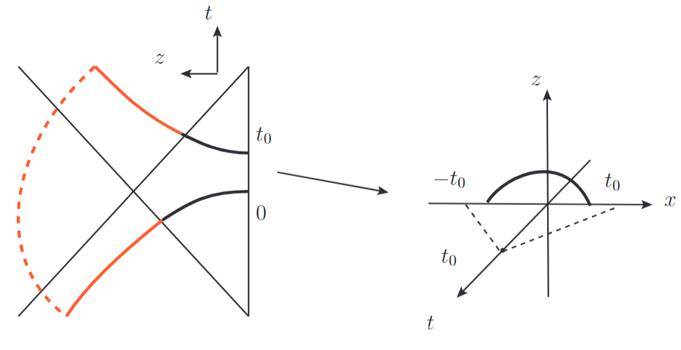
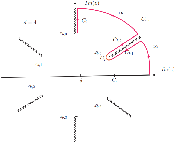
Consider a static spacetime with a horizon. On the boundary, we choose a timelike strip subregion between the time interval (see Fig.2 for illustration). We would like to consider the extreme surfaces anchored to the boundary of the timelike subregion. These extreme surfaces for timelike subregions generally extend into the horizon and approach the singularity of the black hole. However, the RT surfaces for timelike subregions cannot be determined solely by the boundary conditions. In the following, we demonstrate how to construct the specific RT surfaces through analytical continuation of the Euclidean counterparts. An interesting feature is that the RT surfaces naturally extend into the interior of the horizon and the complexified geometry. The area of the RT surface inside the horizon (red line in Fig.1) is related to the area outside the horizon (black line in Fig.1), as well as to the RT surfaces for spacelike regions on the Cauchy surface in the regions . This relation is closely tied to causality. As noted, RT surfaces associated with spacelike subregions lie outside the horizon, suggesting that the relation can be interpreted as a duality between the RT surfaces inside and outside the horizon.
In the context of black hole complementarity, the information inside the black hole can be reconstructed from the exterior degrees of freedom. The algebra of operators inside the horzion can be expressed in terms of exterior operators using the pull-back-push-forward procedure [27, 28]. Roughly speaking, one can re-express the operators in terms of operators in the past and outside the horizon, in the infalling frame. These operators are then evolved in the exterior frame of the black hole, and ultimately, operators inside the black hole can be written as combinations of those outside the horizon. Our results can also be interpreted as a manifestation of black hole complementarity. Although our construction differs significantly, it also follows the causality constraint. The RT surfaces inside the horizon encode information about the black hole’s interior geometry. Our duality relation asserts that this information can be reconstructed using the RT surfaces outside the horizon. This implies that an observer outside the horizon can learn the geometry inside the horizon by measuring the area of the RT surfaces outside the horizon.
2 General setup for the Ryu-Takayanagi surface
In this paper we would like to consider the asymptotically AdSd+1 metric
| (1) |
where we set the AdS radius and . The AdS boundary is at . We assume there exists a Killing horizon with for the Killing vector . The spacetime is divided into regions inside and outside of the horizon as shown in Fig.1. Generally, let us consider a timelike subregion to be a strip between and , denoted by , see Fig.2.

The procedure to construct the RT surface for is as follows. The Euclidean section of the solution (1) can be obtained by . The Euclidean solution is defined for . On the boundary we will consider the subsystem of the strip between and , denoted by . First, we solve for the RT surface associated with the subsystem . By symmetry, we can parameterize the RT surface as and . There exists two conserved constant for the RT surface, which satisfy
| (2) |
In the Euclidean solution , there exists turning point of the RT surface such that . This leads to the condition
| (3) |
By using the conditions and , one could obtain the RT surface in the Euclidean section.
On the other hand if we consider a strip in the Lorentzian metric (1), the RT surface with parametertion and would satisfy a relation similar to (2),
| (4) |
If the separation between and is timelike, there may not exist a real turing point for the RT surface. For exmple, for a timelike strip on with , we have and , thus the solutions of are complex numbers for real . There exists no turning point in the Lorentzian geometry (1). In general, these types of RT surface may pass through the horizon at and possibly extend to the singularity inside the horizon. However, unlike in the Euclidean case, there is no way to fix the values of and in the Lorentzian geometry.
A specific choice is analytical continuation of the RT surface and in Euclidean metric. By comparing the Eq.(2) with the Wick rotation and (2), the conserved constants are fixed by
| (5) |
The turning point would also have a natural analytical result
| (6) |
With these conditions one could solve the RT surface and . We will present some examples later. The procedure outlined above provides a method to construct specific RT surfaces for timelike subregions. As mentioned, these RT surfaces extend into the horizon, offering a way to probe the interior of the black hole. After the analytical continuation (2), there are no turning points in the Lorentzian geometry. This suggests that the RT surface should be extended into the complexified geometry, consistent with the framework proposed in [24]. The area of the RT surface is given by
| (7) | |||||
where is the IR cut-of for the directions, is a path on the complex plane connecting the boundary to the turning point , which is generally a branch point of the integrand in (7).
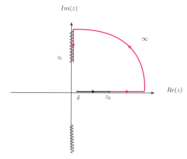
However, there is no principled way to fix the path on the complex -plane. In this paper, we focus on RT surfaces that extend into the horizon. Thus, a natural choice for the path is the one shown in Fig.7 with the path avoiding crossing the branch cut. We can then evaluate the area of the RT surface both inside and outside the horizon.
| (8) |
By definition we have .
3 Connecting with holographic timelike EE and the duality
Before constructing the duality relation in explicit examples, let us explain why we expect such a relation to exist. First, we note that the RT surfaces we have constructed can be interpreted as the holographic timelike EE for the strip subregions in the black hole geometry.
Timelike EE is well-defined and computable in QFTs, even though we may not fully understand its holographic duality. In 2-dimensional QFTs, the EE can be evaluated using the twist operator formalism, which allows the EE to be translated into calculating correlators involving local twist operators in Euclidean QFTs [29]. For timelike subregions, it is natural to define the timelike EE by analytically continuing correlators involving twist operators. Standard methods in QFTs exist for obtaining Lorentzian correlators, as discussed in, e.g., [30].
Our procedure for constructing the RT surface for timelike subregions can be interpreted as the bulk duality of the analytical continuation of twist operator correlators. We demonstrate this procedure with explicit examples, showing that it yields the expected results for timelike EE. In higher dimensions, twist operators are generally non-local. For the strip considered in this paper, the EE can be understood as correlators of non-local operators at the boundaries and . Consider the specific case , as illustrated in Fig.2(b). The timelike EE is associated with the correlator , where the subscript denotes -copies of the theory. By causality, the operators can be decomposed as operators on the Cauchy surface within the region . Consequently, is expected to be represented by correlators on the Cauchy surface, which may also exhibit bulk geometric duality. However, directly decomposing is generally infeasible. In the following, we construct these relations through explicit examples. For the cases we consider, it appears that only the EE and its first-order temporal derivative are required.
To build the relation, we also need a spacelike subregion of the strip with . The corresponding RT surfaces are spacelike. One can evaluate and , which are related solely to information outside the black hole horizon. In the following, we will show that the timelike EE is solely related to this information of spacelike EE. Thus, can be constructed by only using information outside the horizon.
4 Examples
Poincaré coordinate The simplest example is the pure AdS3 in Poincare coordinate with metric . Let us construct the timelike RT surface associated with the interval on the slice . Performing the procedure in previous section, we can obtain . By using (2), we have
| (9) |
One could solve for the RT surface in Lorentzian metric and obtain . There exists a horizon at infity in the Poincaré coordinate. Through some calculations, the area of the RT surface inside the horizon is given by and . By definition, the total length of the RT surface is . It is straightforward to show that the following relation holds,
| (10) |
By RT formula , we obtain the expected result for the timelike EE of the interval . The relation (4) is precisely the timelike and spacelike EE relation constructed in [26] for the CFT vacuum state. Notably, the right-hand side of (4) involves only the RT surfaces outside the horizon ().
BTZ black hole and AdS-Rindler The metric of BTZ black hole is given by
| (11) |
with , where is the horizon of black hole. The singularity is at . We consider the timelike interval on . For the strip we can obtain . By using (2) we have
| (12) |
The turing point is given by . The length of RT surface inside and outside the horizon is given by
| (13) |
See the Appendix for calculation details. The above result yields the expected value for the timelike EE of the interval . It can be shown that the RT surfaces inside and outside the horizon satisfy the relation (4).
For , the metric corresponds to AdS-Rindler coordinates, which cover only a portion of AdS. A causal horizon exists at . The results for AdS-Rindler can be obtained by taking in the BTZ case.
Higher dimensional examples Let us firstly consider the pure AdSd (). The metric is given by (1) with . There exists a horizon at . We consider the strip . As the same procedure we can evaluate the RT surface in the Euclidean metric for the subsystem . We find
| (14) |
With the analytical continuation , we obtain
| (15) |
The turning point can also be obtained by analytical continuation . The area of the RT surface is given by
| (16) |
with . See the Appendix for calculation details. The results are consistent with [24, 31]. For the spacelike strip, the first-order temporal derivative satisfies the following relation [31],
| (17) |
Just like the AdS3 case, the RT surface approaches the horizon and extends into the complexified geometry. The areas of the RT surface inside and outside the horizon can be evaluated. Guided by Eq. (17) and inspired by the AdS3 relation (4), we construct the following equation
| (18) | |||||
One can directly verify the above formula using Eqs. (16) and (17). Notably, in the limit , the formula reduces to the AdS3 case given by Eq. (4).
Now, let us consider the black hole background with . We will still consider the timelike strip . In this case, obtaining an analytical expression for the RT surface area is challenging. However, for small strips satisfying , the problem can be solved perturbatively. In this section, we set and assume , keeping only the leading-order contributions.
Both the timelike and spacelike RT surfaces receive thermal corrections. Let denote the area of the RT surface for the spacelike strip with width on the Cauchy surface . For , the leading-order thermal correction is given by
| (19) |
where represents the thermal correction to the EE of the spacelike strip. The results for are provided in the Appendix.
For the timelike strip we can also obtain the thermal correction. The procedure is same as before. We consider the strip in the Euclidean spacetime. By some calculations we obtain the turining point
| (20) |
where is the constant depending only on . The explicit results are provided in the Appendix. After performing the analytical continuation , we obtain the turning point . We consider the RT surface connecting t0 , with the path on complex -plane chosen similarly to the vacuum case. Given this path, we can then evaluate the area of the RT surface.
| (21) |
where is a constant that depends only on . The explicit results are provided in the Appendix.
We now demonstrate that the relation (17) remains valid in the black hole background. Consider a strip with while ensuring , i.e., a spacelike strip. The holographic EE can be computed perturbatively in this regime. Due to time-reversal symmetry, thermal corrections to the RT surface cannot introduce terms linear in , the leading-order corrections must be at most . Consequently, we find , implying that thermal corrections do not affect the first-order temporal derivative of the spacelike RT surface.
Notably, the corrections to the spacelike and timelike strips differ, i.e., . However, we find that they obey the universal relation
| (22) |
Thus the relation (18) can be modified as
| (23) | |||||
The right-hand side of the above equation only includes information outside the black hole horizon. For there are no thermal corrections on the right-hand side, which is consistent with the formula (4) for the BTZ black hole. We can divide the RT surface for the timelike strip into the inside and outside parts of the horizon. Thus, the RT surface inside the horizon can be constructed using quantities outside the horizon.
5 Discussion
The RT surfaces for timelike subregions can cross the horizon, thereby exploring the interior structure of the black hole. In this paper, we demonstrate how to construct the RT surface for the timelike strip via analytical continuation. We also uncover a duality between the RT surfaces inside and outside the black hole horizon, which can be interpreted as a realization of the concept of black hole complementarity: the information inside the horizon can be reconstructed from the degrees of freedom outside the horizon.
In our construction, it seems necessary to consider the RT surface in the complexified geometry. The role of the complexified geometry in understanding the interior of black holes remains unclear. In this paper, we mainly focus on the static black hole case, where in the general metric (1). If matter is included in the bulk, generally we would have . It has been shown in [9] that the metric near the singularity would resemble a more general Kasner universe [32, 33]. It would be interesting to investigate whether it is possible to construct the duality relation in this case and explore the properties of the singularity through this duality. Additionally, it would be intriguing to explore whether a similar duality exists in the dynamic case, such as when considering the evolution of a black hole with Hawking radiation [34, 35, 36]. The duality relation we have established may provide insight into the relationship between interior degrees of freedom and Hawking radiation.
Acknowledgements We would like to thank Song He, Yan Liu, Rong-Xin Miao, Jia-Rui Sun Tadashi Takayanagi, Run-Qiu Yang, Jiaju Zhang and Yu-Xuan Zhang for useful discussions. WZG would also like to express my gratitude to the Gauge/Gravity Duality 2024 conference, where part of the content of this work was presented. WZG is supposed by the National Natural Science Foundation of China under Grant No.12005070 and the Fundamental Research Funds for the Central Universities under Grants NO.2020kfyXJJS041.
Appendix A RT surfaces for BTZ black hole and AdS-Rindler wedge
In this section, we present the detailed calculations for the area of RT surfaces in the BTZ black hole and the AdS-Rindler wedge.
The metric of the 3-dimensional AdS-Rindler wedge can be seen as the case . The AdS-Rindler coordinate is generally written as
| (24) |
, and . This coordinate system only covers part of the global coordinates. A horizon exists at . By performing the coordinate transformation , the metric becomes
| (25) |
where . The AdS-Rindler coordinate is given by (11) with .
Consider the Euclidean section of the metric of BTZ,
| (26) |
where is the Euclidean time with . The boundary CFT is thus in the thermal state with inverse temperature .
As discussed in the main text, our focus is on the RT surface associated with the timelike interval and the temporal derivative of the RT surface for the spacelike interval . The results presented above pertain to the RT surface corresponding to the spacetime interval between the points and . Our approach involves evaluating these results in the Euclidean metric (26), after which the necessary results are obtained through the analytical continuation .
Let us consider an interval between and on the boundary of Euclidean AdS-Rindler (26). We would like to evaluate the RT surface for , which can be parameterized as and . There exists two conserved constants for the RT surface,
| (27) |
There exists turning point of the geodesic with satisfying and . We also have the relation
| (28) |
and the conditions
| (29) |
With these conditions we can obtain
| (30) |
The length of the geodesic line in the Euclidean section is given by
| (31) |
where and . Taking into the above equation and using RT formula, we obtain the expected result for EE in thermal state with inverse temperature . One could obtain the results for the timelike regions by using the analytical continuation .
We can also obtain the same results by following the procedure discussed in the main text. Consider the interval on the time coordinate . One could obtain , and through analytical continuation. The results are
| (32) |
With these, one can solve for the timelike RT curve . The length of geodesic line is given by
| (33) |
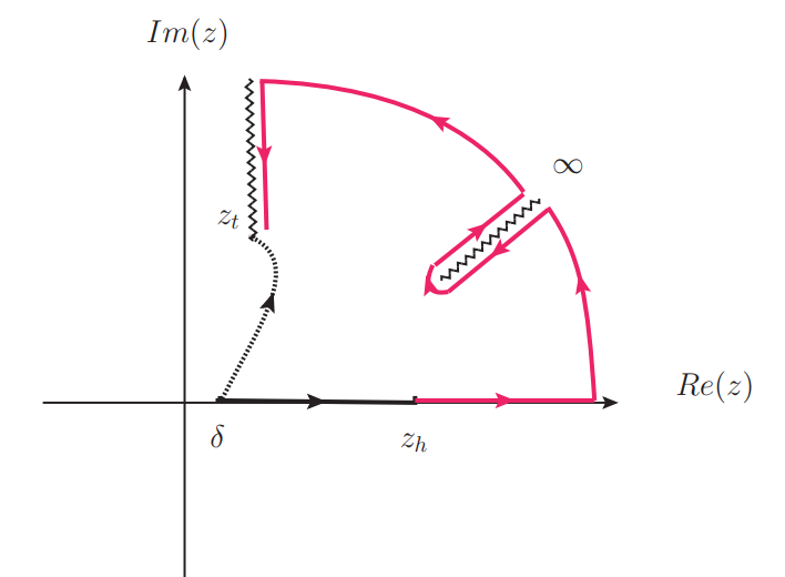
where the path is chosen as shown in Fig.4.
It can be shown directly that the integration yields the correct results for the timelike EE. It is also straightforward to calculate and by the definition (2).
Appendix B Calculation Details for the Higher-Dimensional Strip in the Vacuum State
In this section, we present the details of the calculation for the higher-dimensional strip. For the vacuum state, where , analytical results can be obtained. We will primarily focus on and , highlighting the significant differences between even and odd-dimensional cases.
Consider the strip . By using the Eq.(2) and the conditions that , where is the turning point of the RT surface. One could obtain
| (34) |
with
| (35) |
With the continuation , we find
| (36) |
Note that is real for even , while it is imginary for odd . This leads to a significantly different behavior in odd and even dimensions. The turning point can also be obtained through analytical continuatio n ,
| (37) |
With these results one could evaluate the area for the RT surface. From Eq.(7) we will have
| (38) |
where is the path connecting to .
On the complex -plane the integrand in (38) will have pole at and branch points
| (39) |
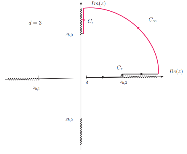
For and , the branch cuts are shown in Fig. 5 and Fig. 6. For a branch cut exists along the coordinate, whereas no such cut appears for . We can now evaluate the area of the RT surface by carefully selecting the integration path . Our goal is to construct an RT surface that extends to the horizon, which, in Poincaré coordinates, is located at . The chosen paths are illustrated in Fig. 5 and Fig. 6.
Let us first consider the case of . It can be easily shown that the contribution from the path is zero. After some calculations, we obtain
| (40) |
where is the UV cut-off. Thus we obtain the area of the RT surface
| (41) |
For the case, it is also easy to show that the contributions from vanish. The contributions from the remaining paths are given by
| (42) |
Thus the area of the RT surface in the case is given by
| (43) |
By our definition we can take as the length of the RT surface outside the horizon. The total area of the RT surface is consistent with the results expected to timelike strip, discussed in [24, 31].
In the vacuum case, the RT surface can be solved analytically. By (2) we have
| (44) |
The integration can be obtained analytically,
In general, the RT surface extends into the complexified geometry, even for real values of .
For with , starts from the boundary . In the region the real part of is constant , but its imaginary part will increase with . Then the imginary part of would be constant in , the real part of will approach to infinity as .
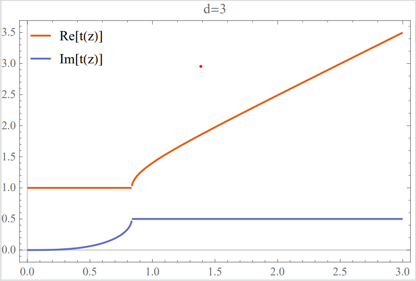
For it is easy to see that the RT surface is real for . Thus the RT surface in this region will explore the Lorentzian metric and approach to the horizon.
Appendix C Calculation Details for the Higher-Dimensional Strip in the Black Hole
In this section, we provide details of the calculation for the RT surface in a higher-dimensional black hole. We set and assume the strip satisfies . This allows us to perturbatively compute the area of the RT surface for the timelike strip. Consider a strip in Euclidean QFTs with . The turning point can be obtained using (2) and (3), along with the condition
| (45) |
One could perturbatively solve as
| (46) |
with
| (47) |
With the analytical continuation , the turning point can be determined.The RT surface can also be obtained perturbatively. The conserved constant can be obtained by using
| (48) |
From Eq.(7) we will have
| (49) |
where is the path connecting to . One can choose the path as in the vacuum case. A more practical approach to evaluating the integral is to first obtain the result for the Euclidean case and then apply analytical continuation.
The area for the RT surface in the Euclidean metric is given by
One could work out this integration perturbatively
Substituting (46) into the above expression, we can obtain the area of the RT surface in the Euclidean metric. By applying the continuation , the results in Lorentzian geometry can be derived. The calculations are straightforward, though the expression is lengthy. We will present some results for in Table.1.
| d | |||
|---|---|---|---|
| 3 | 0 | ||
| 4 | |||
| 5 | |||
| 6 |
References
- [1] C. R. Stephens, G. ’t Hooft and B. F. Whiting, “Black hole evaporation without information loss,” Class. Quant. Grav. 11, 621-648 (1994) [arXiv:gr-qc/9310006 [gr-qc]].
- [2] L. Susskind, L. Thorlacius and J. Uglum, “The Stretched horizon and black hole complementarity,” Phys. Rev. D 48, 3743-3761 (1993) [arXiv:hep-th/9306069 [hep-th]].
- [3] S. Ryu and T. Takayanagi, “Holographic derivation of entanglement entropy from AdS/CFT,” Phys. Rev. Lett. 96, 181602 (2006) [arXiv:hep-th/0603001 [hep-th]].
- [4] V. E. Hubeny, M. Rangamani and T. Takayanagi, “A Covariant holographic entanglement entropy proposal,” JHEP 07, 062 (2007) [arXiv:0705.0016 [hep-th]].
- [5] V. E. Hubeny, “Extremal surfaces as bulk probes in AdS/CFT,” JHEP 07 (2012), 093 [arXiv:1203.1044 [hep-th]].
- [6] N. Engelhardt and A. C. Wall, “Extremal Surface Barriers,” JHEP 03, 068 (2014) [arXiv:1312.3699 [hep-th]].
- [7] T. Hartman and J. Maldacena, “Time Evolution of Entanglement Entropy from Black Hole Interiors,” JHEP 05 (2013), 014 [arXiv:1303.1080 [hep-th]].
- [8] L. Fidkowski, V. Hubeny, M. Kleban and S. Shenker, “The Black hole singularity in AdS / CFT,” JHEP 02 (2004), 014 [arXiv:hep-th/0306170 [hep-th]].
- [9] A. Frenkel, S. A. Hartnoll, J. Kruthoff and Z. D. Shi, “Holographic flows from CFT to the Kasner universe,” JHEP 08 (2020), 003 [arXiv:2004.01192 [hep-th]].
- [10] D. Stanford and L. Susskind, “Complexity and Shock Wave Geometries,” Phys. Rev. D 90, no.12, 126007 (2014) [arXiv:1406.2678 [hep-th]].
- [11] A. R. Brown, D. A. Roberts, L. Susskind, B. Swingle and Y. Zhao, “Holographic Complexity Equals Bulk Action?,” Phys. Rev. Lett. 116, no.19, 191301 (2016) [arXiv:1509.07876 [hep-th]].
- [12] K. Doi, J. Harper, A. Mollabashi, T. Takayanagi and Y. Taki, “Pseudoentropy in dS/CFT and Timelike Entanglement Entropy,” Phys. Rev. Lett. 130, no.3, 031601 (2023) [arXiv:2210.09457 [hep-th]].
- [13] Y. Nakata, T. Takayanagi, Y. Taki, K. Tamaoka and Z. Wei, “New holographic generalization of entanglement entropy,” Phys. Rev. D 103 (2021) no.2, 026005 doi:10.1103/PhysRevD.103.026005 [arXiv:2005.13801 [hep-th]].
- [14] S. J. Olson and T. C. Ralph, “Entanglement between the future and past in the quantum vacuum,” Phys. Rev. Lett. 106 (2011), 110404 [arXiv:1003.0720 [quant-ph]].
- [15] J. Cotler, C. M. Jian, X. L. Qi and F. Wilczek, “Superdensity Operators for Spacetime Quantum Mechanics,” JHEP 09 (2018), 093 [arXiv:1711.03119 [quant-ph]].
- [16] P. Wang, H. Wu and H. Yang, “Fix the dual geometries of deformed CFT2 and highly excited states of CFT2,” Eur. Phys. J. C 80 (2020) no.12, 1117 [arXiv:1811.07758 [hep-th]].
- [17] A. Lerose, M. Sonner and D. A. Abanin, “Scaling of temporal entanglement in proximity to integrability,” Phys. Rev. B 104 (2021) no.3, 035137 [arXiv:2104.07607 [quant-ph]].
- [18] G. Giudice, G. Giudici, M. Sonner, J. Thoenniss, A. Lerose, D. A. Abanin and L. Piroli, “Temporal Entanglement, Quasiparticles, and the Role of Interactions,” Phys. Rev. Lett. 128 (2022) no.22, 220401 [arXiv:2112.14264 [cond-mat.stat-mech]].
- [19] K. Narayan, “de Sitter space, extremal surfaces, and time entanglement,” Phys. Rev. D 107 (2023) no.12, 126004 doi:10.1103/PhysRevD.107.126004 [arXiv:2210.12963 [hep-th]].
- [20] B. Liu, H. Chen and B. Lian, “Entanglement entropy of free fermions in timelike slices,” Phys. Rev. B 110 (2024) no.14, 144306 [arXiv:2210.03134 [cond-mat.stat-mech]].
- [21] P. Glorioso, X. L. Qi and Z. Yang, “Space-time generalization of mutual information,” JHEP 05 (2024), 338 [arXiv:2401.02475 [quant-ph]].
- [22] A. Milekhin, Z. Adamska and J. Preskill, “Observable and computable entanglement in time,” [arXiv:2502.12240 [quant-ph]].
- [23] K. Doi, J. Harper, A. Mollabashi, T. Takayanagi and Y. Taki, “Timelike entanglement entropy,” JHEP 05, 052 (2023) [arXiv:2302.11695 [hep-th]].
- [24] M. P. Heller, F. Ori and A. Serantes, “Geometric interpretation of timelike entanglement entropy,” [arXiv:2408.15752 [hep-th]].
- [25] T. Anegawa and K. Tamaoka, “Black hole singularity and timelike entanglement,” JHEP 10 (2024), 182 [arXiv:2406.10968 [hep-th]].
- [26] W. z. Guo, S. He and Y. X. Zhang, “Relation between timelike and spacelike entanglement entropy,” [arXiv:2402.00268 [hep-th]].
- [27] I. Heemskerk, D. Marolf, J. Polchinski and J. Sully, “Bulk and Transhorizon Measurements in AdS/CFT,” JHEP 10 (2012), 165 [arXiv:1201.3664 [hep-th]].
- [28] L. Susskind, “The Transfer of Entanglement: The Case for Firewalls,” [arXiv:1210.2098 [hep-th]].
- [29] P. Calabrese and J. L. Cardy, “Entanglement entropy and quantum field theory,” J. Stat. Mech. 0406 (2004), P06002 [arXiv:hep-th/0405152 [hep-th]].
- [30] T. Hartman, S. Jain and S. Kundu, “Causality Constraints in Conformal Field Theory,” JHEP 05 (2016), 099 [arXiv:1509.00014 [hep-th]].
- [31] J. Xu and W. z. Guo, “Imaginary part of timelike entanglement entropy,” JHEP 02 (2025), 094 [arXiv:2410.22684 [hep-th]].
- [32] E. Kasner, “Geometrical theorems on Einstein’s cosmological equations,” Am. J. Math. 43 (1921), 217-221
- [33] V. A. Belinski and I. M. Khalatnikov, “Effect of Scalar and Vector Fields on the Nature of the Cosmological Singularity,” Sov. Phys. JETP 36 (1973), 591
- [34] A. Almheiri, N. Engelhardt, D. Marolf and H. Maxfield, “The entropy of bulk quantum fields and the entanglement wedge of an evaporating black hole,” JHEP 12, 063 (2019) [arXiv:1905.08762 [hep-th]].
- [35] A. Almheiri, R. Mahajan, J. Maldacena and Y. Zhao, “The Page curve of Hawking radiation from semiclassical geometry,” JHEP 03, 149 (2020) [arXiv:1908.10996 [hep-th]].
- [36] A. Almheiri, T. Hartman, J. Maldacena, E. Shaghoulian and A. Tajdini, “The entropy of Hawking radiation,” Rev. Mod. Phys. 93, no.3, 035002 (2021) [arXiv:2006.06872 [hep-th]].