A Dynamic Approach to Linear Statistical Calibration with an Application in Microwave Radiometry
Abstract
The problem of statistical calibration of a measuring instrument can be framed both in a statistical context as well as in an engineering context. In the first, the problem is dealt with by distinguishing between the “classical" approach and the “inverse" regression approach. Both of these models are static models and are used to estimate “exact" measurements from measurements that are affected by error. In the engineering context, the variables of interest are considered to be taken at the time at which you observe it. The Bayesian time series analysis method of Dynamic Linear Models (DLM) can be used to monitor the evolution of the measures, thus introducing an dynamic approach to statistical calibration. The research presented employs the use of Bayesian methodology to perform statistical calibration. The DLM’s framework is used to capture the time-varying parameters that maybe changing or drifting over time. Two separate DLM based models are presented in this paper. A simulation study is conducted where the two models are compared to some well known ’static’ calibration approaches in the literature from both the frequentist and Bayesian perspectives. The focus of the study is to understand how well the dynamic statistical calibration methods performs under various signal-to-noise ratios, . The posterior distributions of the estimated calibration points as well as the coverage intervals are compared by statistical summaries. These dynamic methods are applied to a microwave radiometry dataset.
1. Introduction
Calibrating measurement instruments is a important problem that engineers frequently need to address. There exist several statistical methods that address this problem that are based on a simple linear regression approach. In tradition simple linear regression the goal is to relate a known value of X to a uncertain value of Y using a linear relationship. In contrast, the statistical calibration problem seeks to utilize a simple linear regression model to relate a known value of Y to an uncertain value of X. This is why statistical calibration is sometimes called inverse regression due to its relationship to simple linear regression (Osborne 1991; Ott and Longnecker 2009). Recall in linear regression the model is given as follows:
| (1) |
where Y is a response vector, X is a matrix of independent variables with total model parameters, is a vector of unknown fixed parameters and is a vector of uncorrelated error terms with zero mean (Myers 1990; Draper and Smith 1998; Montgomery et al. 2012). It is assumed that the value of the predictor variable X = x are nonrandom and observed with negligible error, while the error terms are random variables with mean zero and constant variance (Myers 1990).
Typically, in regression, of interest is the estimation of the parameter vector; , and possibly the prediction of a future value corresponding to a new value. The prediction problem is relatively straightforward, due to the fact that a future value can be made directly by substituting into (1) with .
For the statistical calibration problem let be the known observed value of the response and be the corresponding regressor, which is to be estimated. This problem is conducted in two stages: first measurement pairs of data is observed and a simple linear regression line is fit by estimating ; secondly, observations of the response are observed, all corresponding to a single (Özyurt and Erar 2003). Since is fixed, inferences are different than those in a traditional regression (or prediction) problem (Osborne 1991; Eno 1999; Eno and Ye 2000).
1. Classical Calibration Methods
Eisenhart (1939) offered the first solution to the calibration problem, and is commonly known as the estimator to the linear calibration problem. They assumed that the relationship between and was of a simple linear form:
The estimated regression line for the first stage of the experiment is given by
| (2) |
where and are the least squares estimate of and , respectively. Using the data collected at the first stage of experimentation, Eisenhart (1939) inverts Equation (2) to estimate the unknown regressor value for an observed response value , by:
| (3) |
where denotes the estimator for . Since division by is used there is an implicit assumption that .
Assuming that , Brown (1993) describes the following interval estimate corresponding to Eisenhart (1939):
where
Krutchkoff (1967) proposed a competitive approach to Eisenhart’s (1939) classical linear calibration solution, which he called the regression calibration method and is written as:
where and are the parameters in the linear relationship and are independent identically distributed measurement errors with a zero mean and finite variance. Here and are estimated via least squares. The unknown can be estimated directly by substituting into the fitted equation:
| (4) |
We let denote the estimator of . The confidence interval for can be written as
where
Krutchkoff (1967) used a simulation study, where he found that the mean squared error of estimation for was uniformly less for this estimator versus the classical estimator. The inverse approach was later supported by Lwin and Maritz (1982). For criticisms of Krutchkoff’s (1967) approach such as bias see Osborne (1991).
2. Bayesian Calibration Methods
The first noted Bayesian solution to the calibration problem was presented by Hoadley (1970). His work was motivated by the unanswered question in the Frequentist community of whether is zero (or close to zero). Hoadley (1970) justified the use of the estimator (Krutchkoff, 1967) by considering the ususal -statistic to test the hypothesis that where ,
The assumption made by Hoadley (1970) reflects that is random and a priori independent of , so that the joint prior distribution of . Hoadley (1970) first assumed that had a uniform distribution,
but the prior distribution for was not given.
Hoadley (1970) shows for (one observation at the prediction stage), that if has a prior density from a Student t distribution with degrees of freedom, a mean of 0, and a scale parameter
the posterior distribution is
| (5) |
where is the inverse estimator given by (4) and .
Hunter and Lamboy (1981) also considered the calibration problem from a Bayesian point of view and is similar to that of Hoadley (1970) because both assume the prior distribution to be
where which is the predicted . The primary difference between their approach and the approach of Hoadley (1970) is that a priori they assume that and are independent while Hoadley (1970) assumed a priori that and are independent.
Hunter and Lamboy (1981) uses an approximation to the posterior distribution of the unknown regressor by
| (6) |
where
with being the classical estimator given in Equation (3), denote the element of the row and column from variance-covariance matrix of the joint posterior density of (, , ).
The remainder of this paper is organized as follows. Section 2 presents the development of the dynamic approaches to the statistical calibration problem. In Section 3 the results from the simulation study where the dynamics methods are evaluated along with the static approaches are presented. In Section 4 the proposed methods are applied to microwave radiometer data. In Section 5 future work and other considerations are given.
2. Dynamic Calibration Approach
Traditional calibration methods assume the regression relationship is “static” in time. In many cases this is false, for example in microwave radiometry the static nature of the relationship is known to change across time. A dynamic approach can be created by letting the regression coefficients vary through time,
where and is known as the error.
The model may have different defining parameters at different times. One approach is to model and by using random walk type evolutions for the defining parameters, such as:
where and are independent zero-mean error terms with finite variances. At any time the calibration problem is given by:
Bayesian Dynamic Linear Models (DLMs) approach of West et al. (1985); West and Harrison (1997) can be employed to achieve this goal. Recall the DLM framework is:
for some prior mean and variance with the vector of error terms, and independent across time and at any time.
To update the model through time West and Harrison (1997) give the following method:
-
(a)
Posterior distribution at : For some mean and variance ,
. -
(b)
Prior distribution at time : , where
and . -
(c)
One-step forecast: , where
and . -
(d)
Posterior distribution at time : , with
and
where
and .
The DLM framework is used to establish the evolving relationship between the fixed design matrix and by estimating , which is a matrix of time-varying regression coefficients and . For our calibration situation is a matrix of responses and is a known () system matrix. The error and are independent normally distributed random matrices with zero mean and constant variance-covariance matrices E and W. For simplification is set equal to , is set equal to and is . The past information is contained in the set .
We specify a prior in the first stage of calibration for the unknown variances and derive an algorithm to draw from the posterior distribution of the unknown parameters,
The second stage of the calibration experiment consists of using the joint posterior distribution to derive for each draw of . The estimator for the parameter of interest, , is defined in a manner akin to Eisenhart (1939); Hunter and Lamboy (1981); Eno (1999), where
| (7) |
In the final stage of the calibration experiment, the posterior distribution summary statistics are gathered at each time point . The posterior median and credible intervals are taken for each across the draws of . The result of the dynamic calibration experiment is a time series of calibration distributions across time. We will be able to observe the distributional changes of the system with respect to the calibration reference.
The proposed calibration estimator is developed by first considering the joint posterior distribution .
We let denote the vector of unknown DLM dispersion parameters where . The prior information for the dispersion parameters is described by a prior density which summarizes what is known about the variance parameters before any data are observed. Using the Bayesian inferential approach, the prior information about the parameters must be combined with information contained in the data. The information provided by the data is captured by the likelihood functions, and for the observation equation and the system equation, respectively. The combined information is described by the posterior density using the Bayes theorem (Bernardo and Smith 1994) as
For our calibration problem it is believe that . To deal with the variance relationship we specify the following prior distributions:
| (8) | |||||
| (9) |
Prior distributions (8) and (9) ensures the system variance to be less than the observation variance.
Since these are proper prior distributions the resulting posterior distribution will also be proper.
In the first stage of calibration, the joint distribution of the observations, states, and unknown parameters is as follows:
where the likelihood for the observation equation is
and the likelihood for the system equation is
Given the joint distribution above, the posterior distribution is
| (10) |
where
| (11) |
and (i.e. is the cumulative mean of the observations up to time ) and . Samples from the posterior distribution in Equation (10) are drawn by implementing the Sampling Importance Resampling (Albert 2007; Givens and Hoeting 2005) approach.
The development of the estimator in Equation (11) is deterministic in approach. We present a fully Bayesian approach to dynamic calibration that incorporates the uncertainty in estimation. The second dynamic calibration model is derived by Bayes’ theorem
where is the posterior distribution for . The prior belief for the calibration values is denoted as with the denoting the likelihood function.
The objective of any Bayesian approach is to obtain the posterior distribution from which inferences can be made. Here the desired posterior is
| (12) |
which must be dynamic through time. We determine the posterior distribution (12) in a similiar manner as described above in Equations (10) and (11). In the first stage of the calibration experiment the data is scaled and centered, therefore setting the intercept equal to zero and the reference measurements centered at zero. Centering of the data is used to reduce the parameter space. The posterior distribution can be thought of as:
| (13) |
with representing the transformed calibrated value at time and , where is the cumulative mean of the observations. Given this information we define the prior distribution
The posterior density in Equation (13) is defined as
| (14) |
where . Applying Bayes theorem and completing the square, the posterior distribution is
| (15) |
with
and
where tr( . ) denotes trace of the one-step forecast variance-covariance matrix. We derive the posterior in Equation (12) by drawing from Equation (15) and transforming the data back to the original scale as so:
| (16) |
where is the mean of the reference measurements vector and is the standard deviation of the reference measurements vector.
The dynamic calibration algorithm is developed for both of the approaches using R (R Development Core Team, 2013) and is conducted as below.
-
a.
Data are scaled and shifted such that , and intercept , where for all (i.e. is the cumulative mean up to time );
-
b.
Estimate for the proposal sample is calculated ;
- c.
-
d.
Calculate log-likelihood density weights, , for each pair
Sampling Importance Resampling (SIR) is used to simulate samples of by accepting a subset of from the proposal density to be distributed according to the posterior density with candidate density .
-
a.
Calculate the standardized importance weights, , where for the proposal sample;
-
b.
Sample calibrated time series from the proposal values with replacement given probabilities where
Rescale calibrated time series to original scale by Equation (16) and take summary statistics (i.e. medians and credible sets) across each time .
3. Simulation Study
A simulation study, mirroring the microwave radiometer example in Section 4, considers the performance of the proposed dynamic calibration approaches to the static approaches discussed in Section 1. For notation, the calibration methods are labelled as follows:
-
1.
is the first deterministic dynamic calibration model given in Equation (11);
-
2.
is the Bayesian dynamic calibration model given by Equation (15);
-
3.
is the approach of Eisenhart (1939) defined in Equation (3);
-
4.
is the approach of Krutchkoff (1967) defined in Equation (4);
-
5.
is Hoadley (1970) Bayesian approach as defined in Equation (5);
-
6.
is Hunter & Lamboy (1981) Bayesian approach as defined in Equation (6).
Note that static methods , , , and require that model fitting and the calibration take place after all the data has been collected. This is in contrast to the dynamic methods that both fit the model and generate calibrated values each point through time and hence provide a near real time calibration. In order to assess the performance of the calibration methods 100 datasets were randomly generated according to
| (17) |
where is a known fixed design matrix of reference values. The number of references measurements used in the study was two and five. The reference values at the first stage of the simulation study were equally spaced, covering the interval . For the two reference case, the fixed design matrix is
and for the five reference case the design matrix is
The vector of regression parameters, , are randomly drawn from a multivariate normal distribution with mean vector and variance-covariance matrix, for , where . For each , the random multivariate error vector is
where the errors are mutually independent. The relationship of the values for and will be explained later.
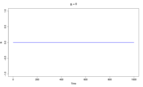
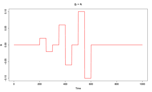
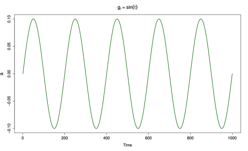
The dynamic and static calibration methods are evaluated for three distinct system fluctuations, , on the regression slope calculated in the first stage of calibration. The value is added to , therefore making Equation (17)
for the calibration references. The three scenarios for the fluctuations are as follows:
-
1.
a constant zero () for all , representing a stable system;
-
2.
a stable system with abrupt shifts ( in system, with ; and
-
3.
a constant sinusoidal fluctuation () for all .
Figure 1) explains the relationship of across time.
The magnitude and relationship of the variance pair influence the DLM and hence to study this influence we set the variances to reflect various signal-to-noise ratios. The true values for and used in the simulation study are and , respectively. Petris et al. (2009) define the signal-to-noise ratio as follows:
The signal-to-noise ratios in the simulation study were examined in two sets. First, is set equal to 10, 100, and 1000. Next, the ratio was set to equal 2, 20, and 200. The variety of values allow us to examine the methods under different levels of noise. Each simulation is repeated 100 times for both the 2- and 5-point calibration models, thus providing us with 36 possible models for examination from the settings of .
After the data was fit with each of the methods we considered the following measures for assessing the performance of the dynamic methods compared to the familiar static approaches: (1) average mean square error; (2) average coverage probability; and (3) average interval width. For each of the simulated data sets, the mean squared error () is calculated as
The are averaged across the 100 simulated data sets thus deriving an average mean squared error () as
The coverage probability based on the coverage interval is estimated for all of the calibration methods. The coverage interval for the dynamic and static Bayesian approaches is the credible interval and the confidence interval is used for the frequentist methods. Note, that for credible intervals is the 0.025 posterior quantile for , and is the 0.975 posterior quantile for , where is the true value of the calibration target from the second stage of experimentation, then is a credible interval. The coveraged probability () is calculated as such
where
The average coverage probability () is calculated by averaging across the number of replications in the simulation study, where
Another quantity of interest to compare the average interval widths () for the methods, where the average interval widths () across the simulated time series is calculated as follows:
with the average interval width across the simulation study given as
where is the average interval width for the simulation replicate. The performance of the dynamic calibration approaches will be assess using the average coverage probability (), average interval width () and average mean square ().
We consider the performance of the methods under two conditions: interpolation and extrapolation. Interpolation case is of interest to understand how the method performed when the calibrated time series is within the range of the reference values, [20, 100]. Extrapolation case also conducted to examine the methods when falls outside of the range of the calibration references, where . While it not preferable to do extrapolation in the regression case, it is often done in practice in microwave radiometry.
All simulations were carried out on the Compile server running (R Development Core Team, 2013) at Virginia Commonwealth University. The Compile server has a Linux OS with 16 CPU cores and 32 GB Ram. Each iteration in the study took approximately 15 minutes with a total of 25.63 hours.
1. Interpolation case
In the following tables, the simulation results for the dynamic and static calibration methods are provided. The results of simulation studies provide insight into the properties of the calibration approaches. The results in Tables 1 and 1 indicate that all of the estimators do a good job at approximating the true values of when the gain flucuation is set to 0. Even in this case we see as the signal-to-noise ratio increases so does the values. All of the methods have an average coverage probability of 1 or close. The high coverage rate is of no surprise for a stable system. There does not appear to be an advantage by including more reference measurements (i.e 2- or 5-points) in the model when the system is stable in time. The clear difference is the values for the dynamic methods compared to the static methods. In Tables 1 and 1 when and , the interval for the dynamic methods is wider than those of the four static methods but as increases the interval width of the dynamic methods remain nearly unchanged as the interval widths for the static methods are 4 to 5 times wider.
The simulation results for the stepped gain fluctuations are provided in Tables 1 and 1. Clearly the presence of the stepped has an effect on the fit of the models. The results in Tables 1 show that in nearly all cases, the two dynamic methods and have values smaller than the two static Bayesian approaches. The values for the dynamic methods are reasonably lower for . When , notice the dynamic models and have smaller average mean square errors smaller than the static method . The average coverage probability is comparable for all of the methods and number of references. The dynamic methods consistently have shorter interval widths. The widths of the 95% credible intervals for and is not affected by the increases in .
| Constant | ||||||||||
| Ref. | Model | AvMSE | AvCP | AvIW | AvMSE | AvCP | AvIW | AvMSE | AvCP | AvIW |
| 2 | 0.0008 | 0.995 | 2.519 | 0.0035 | 0.983 | 2.523 | 0.0307 | 0.939 | 2.517 | |
| 0.0012 | 1.000 | 3.782 | 0.0038 | 1.000 | 3.782 | 0.0308 | 1.000 | 3.782 | ||
| 0.0001 | 1.000 | 1.224 | 0.0012 | 1.000 | 3.868 | 0.0123 | 1.000 | 12.229 | ||
| 0.0001 | 1.000 | 1.223 | 0.0016 | 1.000 | 3.863 | 0.0335 | 1.000 | 12.168 | ||
| 0.0002 | 0.997 | 1.182 | 0.0022 | 1.000 | 3.866 | 0.0386 | 1.000 | 12.177 | ||
| 0.0014 | 1.000 | 1.458 | 0.0139 | 1.000 | 4.606 | 0.1391 | 1.000 | 14.565 | ||
| 5 | 0.0008 | 0.995 | 2.496 | 0.0035 | 0.983 | 2.509 | 0.0307 | 0.941 | 2.514 | |
| 0.0013 | 1.000 | 3.983 | 0.0039 | 1.000 | 3.983 | 0.0307 | 1.000 | 3.983 | ||
| 0.0001 | 1.000 | 1.223 | 0.0012 | 1.000 | 3.865 | 0.0123 | 1.000 | 12.220 | ||
| 0.0001 | 1.000 | 1.222 | 0.0022 | 1.000 | 3.860 | 0.0813 | 1.000 | 12.113 | ||
| 0.0002 | 1.000 | 1.223 | 0.0023 | 1.000 | 3.861 | 0.0792 | 1.000 | 12.116 | ||
| 0.0014 | 1.000 | 1.457 | 0.0139 | 1.000 | 4.604 | 0.1069 | 1.000 | 10.748 | ||
| Constant | ||||||||||
| Ref. | Model | AvMSE | AvCP | AvIW | AvMSE | AvCP | AvIW | AvMSE | AvCP | AvIW |
| 2 | 0.0012 | 0.992 | 2.519 | 0.0041 | 0.981 | 2.520 | 0.0323 | 0.939 | 2.528 | |
| 0.0015 | 1.000 | 3.782 | 0.0044 | 1.000 | 3.782 | 0.0325 | 1.000 | 3.782 | ||
| 0.0001 | 1.000 | 1.230 | 0.0010 | 1.000 | 3.871 | 0.0114 | 1.000 | 12.231 | ||
| 0.0001 | 1.000 | 1.229 | 0.0012 | 1.000 | 3.866 | 0.0314 | 1.000 | 12.170 | ||
| 0.0001 | 1.000 | 1.230 | 0.0019 | 1.000 | 3.869 | 0.0371 | 1.000 | 12.179 | ||
| 0.0190 | 1.000 | 1.155 | 0.0243 | 1.000 | 3.767 | 0.1381 | 1.000 | 14.567 | ||
| 5 | 0.0011 | 0.992 | 2.508 | 0.0041 | 0.981 | 2.510 | 0.032 | 0.939 | 2.514 | |
| 0.0017 | 1.000 | 3.983 | 0.0045 | 1.000 | 3.983 | 0.032 | 1.000 | 3.983 | ||
| 0.0001 | 1.000 | 1.228 | 0.0010 | 1.000 | 3.868 | 0.011 | 1.000 | 12.222 | ||
| 0.0001 | 1.000 | 1.227 | 0.0019 | 1.000 | 3.863 | 0.081 | 1.000 | 12.114 | ||
| 0.0001 | 1.000 | 1.227 | 0.0021 | 1.000 | 3.864 | 0.082 | 1.000 | 12.118 | ||
| 0.0013 | 1.000 | 1.462 | 0.0137 | 1.000 | 4.607 | 0.138 | 1.000 | 14.560 | ||
| Stepped | ||||||||||
| Ref. | Model | AvMSE | AvCP | AvIW | AvMSE | AvCP | AvIW | AvMSE | AvCP | AvIW |
| 2 | 0.0191 | 0.961 | 2.509 | 0.0198 | 0.953 | 2.506 | 0.0406 | 0.926 | 2.543 | |
| 0.0196 | 1.000 | 3.782 | 0.0201 | 1.000 | 3.782 | 0.0408 | 1.000 | 3.783 | ||
| 0.0001 | 1.000 | 9.094 | 0.0004 | 1.000 | 9.813 | 0.0094 | 1.000 | 15.209 | ||
| 0.0046 | 1.000 | 9.065 | 0.0073 | 1.000 | 9.779 | 0.0528 | 1.000 | 15.098 | ||
| 0.0859 | 1.000 | 9.072 | 0.0838 | 1.000 | 9.786 | 0.1866 | 1.000 | 15.109 | ||
| 0.1399 | 1.000 | 10.830 | 0.0823 | 1.000 | 11.687 | 0.1836 | 1.000 | 18.115 | ||
| 5 | 0.0191 | 0.961 | 2.510 | 0.0197 | 0.954 | 2.511 | 0.0405 | 0.924 | 2.516 | |
| 0.0196 | 1.000 | 3.983 | 0.0201 | 1.000 | 3.983 | 0.0405 | 1.000 | 3.983 | ||
| 0.0001 | 1.000 | 9.087 | 0.0004 | 1.000 | 9.806 | 0.0094 | 1.000 | 15.199 | ||
| 0.0184 | 1.000 | 9.041 | 0.0267 | 1.000 | 9.749 | 0.1620 | 1.000 | 14.995 | ||
| 0.0199 | 1.000 | 9.044 | 0.0267 | 1.000 | 9.752 | 0.1559 | 1.000 | 14.999 | ||
| 0.0706 | 1.000 | 10.826 | 0.0618 | 1.000 | 8.625 | 0.1742 | 1.000 | 15.091 | ||
| Stepped | ||||||||||
| Ref. | Model | AvMSE | AvCP | AvIW | AvMSE | AvCP | AvIW | AvMSE | AvCP | AvIW |
| 2 | 0.0209 | 0.957 | 2.520 | 0.0219 | 0.950 | 2.522 | 0.0436 | 0.921 | 2.526 | |
| 0.0214 | 1.000 | 3.782 | 0.0222 | 1.000 | 3.782 | 0.0438 | 1.000 | 3.782 | ||
| 0.0001 | 1.000 | 9.103 | 0.0003 | 1.000 | 9.822 | 0.0086 | 1.000 | 15.216 | ||
| 0.0047 | 1.000 | 9.075 | 0.0073 | 1.000 | 9.788 | 0.0511 | 1.000 | 15.105 | ||
| 0.0084 | 1.000 | 9.081 | 0.0115 | 1.000 | 9.795 | 0.0601 | 1.000 | 15.116 | ||
| 0.0709 | 1.000 | 10.842 | 0.0826 | 1.000 | 11.698 | 0.2054 | 1.000 | 18.122 | ||
| 5 | 0.0209 | 0.957 | 2.509 | 0.0218 | 0.949 | 2.511 | 0.0436 | 0.920 | 2.516 | |
| 0.0214 | 1.000 | 3.983 | 0.0221 | 1.000 | 3.983 | 0.0435 | 1.000 | 3.983 | ||
| 0.0001 | 1.000 | 9.096 | 0.0003 | 1.000 | 9.815 | 0.0086 | 1.000 | 15.205 | ||
| 0.0185 | 1.000 | 9.050 | 0.0267 | 1.000 | 9.758 | 0.1616 | 1.000 | 15.002 | ||
| 0.0199 | 1.000 | 9.053 | 0.0281 | 1.000 | 9.761 | 0.1641 | 1.000 | 15.006 | ||
| 0.0708 | 1.000 | 10.836 | 0.0825 | 1.000 | 11.693 | 0.2052 | 1.000 | 18.114 | ||
| Sinusoidal | ||||||||||
| Ref. | Model | AvMSE | AvCP | AvIW | AvMSE | AvCP | AvIW | AvMSE | AvCP | AvIW |
| 2 | 4.4088 | 0.628 | 2.657 | 4.4794 | 0.629 | 2.648 | 4.7214 | 0.638 | 2.681 | |
| 4.4002 | 0.829 | 3.783 | 4.4708 | 0.825 | 3.783 | 4.7123 | 0.810 | 3.783 | ||
| 0.0001 | 1.000 | 21.980 | 0.0012 | 1.000 | 22.307 | 0.0123 | 1.000 | 25.206 | ||
| 0.1541 | 1.000 | 21.665 | 0.1670 | 1.000 | 21.978 | 0.2943 | 1.000 | 24.738 | ||
| 0.1689 | 0.975 | 20.933 | 0.1868 | 1.000 | 21.994 | 0.3174 | 1.000 | 24.757 | ||
| 0.4127 | 1.000 | 26.178 | 0.4258 | 1.000 | 26.567 | 0.5531 | 1.000 | 30.020 | ||
| 5 | 4.4087 | 0.628 | 2.646 | 4.4793 | 0.630 | 2.648 | 4.7214 | 0.635 | 2.653 | |
| 4.3906 | 0.845 | 3.984 | 4.4609 | 0.839 | 3.984 | 4.7023 | 0.824 | 3.984 | ||
| 0.0001 | 1.000 | 21.964 | 0.0012 | 1.000 | 22.291 | 0.0123 | 1.000 | 25.188 | ||
| 0.5810 | 1.000 | 21.371 | 0.6218 | 1.000 | 21.671 | 1.0152 | 1.000 | 24.306 | ||
| 0.5956 | 1.000 | 21.377 | 0.5909 | 1.000 | 21.678 | 0.9628 | 1.000 | 24.314 | ||
| 0.4123 | 1.000 | 26.166 | 0.3087 | 1.000 | 18.973 | 0.4658 | 1.000 | 25.009 | ||
| Sinusoidal | ||||||||||
| Ref. | Model | AvMSE | AvCP | AvIW | AvMSE | AvCP | AvIW | AvMSE | AvCP | AvIW |
| 2 | 4.4504 | 0.625 | 2.658 | 4.5213 | 0.628 | 2.660 | 4.7643 | 0.6331 | 2.665 | |
| 4.4419 | 0.828 | 3.783 | 4.5127 | 0.823 | 3.783 | 4.7553 | 0.8083 | 3.783 | ||
| 0.0001 | 1.000 | 21.968 | 0.0010 | 1.000 | 22.295 | 0.0114 | 1.000 | 25.196 | ||
| 0.1538 | 1.000 | 21.653 | 0.1672 | 1.000 | 21.966 | 0.2896 | 1.000 | 24.729 | ||
| 0.1732 | 1.000 | 21.669 | 0.1867 | 1.000 | 21.982 | 0.3127 | 1.000 | 24.748 | ||
| 0.4122 | 1.000 | 26.164 | 0.4253 | 1.000 | 26.553 | 0.5518 | 1.000 | 30.008 | ||
| 5 | 4.4504 | 0.625 | 2.647 | 4.5213 | 0.627 | 2.648 | 4.7643 | 0.633 | 2.654 | |
| 4.4322 | 0.844 | 3.984 | 4.5029 | 0.838 | 3.984 | 4.7451 | 0.823 | 3.984 | ||
| 0.0001 | 1.000 | 21.952 | 0.0010 | 1.000 | 22.278 | 0.0114 | 1.000 | 25.178 | ||
| 0.5799 | 1.000 | 21.359 | 0.6206 | 1.000 | 21.660 | 1.0133 | 1.000 | 24.297 | ||
| 0.5851 | 1.000 | 21.366 | 0.6256 | 1.000 | 21.667 | 1.0183 | 1.000 | 24.304 | ||
| 0.4119 | 1.000 | 26.152 | 0.4247 | 1.000 | 26.541 | 0.5513 | 1.000 | 29.995 | ||
The results provided in Tables 1 and 1 summarize the performance of the methods when the gain fluctuation is sinusoidal noise. The results for values of 10, 100, and 1000 are given in Table 1 with and 200 given in Table 1. When is sinusoidal, the values for the dynamic methods are consistently larger than any of the static methods. For all of the chosen values, the is considerably lower than the opposing methods. The dynamic methods still have average interval widths extremely shorter than any of the static methods. The is constant across the signal-to-noise ratios.
The simulation study shows that methods and do a good job at estimating calibrated values that are interior to the range of reference measurements. Both methods display high coverage probabilities in the presence of drifting parameters. For the three possible gain fluctuations, the interval widths for the dynamic methods were consistently shorter than the static calibration approaches. When fitting data where there is a definite linear relationship the dynamic methods are invariant to the number of reference measurements. When using the proposed methods in this paper, not much will be gained by using more than 2 reference measurements. Overall, when interpolating to estimate , the dynamic methods outperform the static Bayesian approaches across the different signal-to-noise ratios. In the following section the performance of the dynamic methods are assessed when the calibrated values fall outside of the range of reference measurements.
2. Extrapolation case
At this point in the paper we examine the calibration approaches when the calibrated values are outside of the reference measurements. The range of the measurement references is from 20 to 100. The true behaved as a random walk bounded between 100 and 110. We assessed the performance of the dynamic methods under three possible gain fluctuation patterns. First, the simulation study is conducted without the presence of additional gain fluctuation (i.e. ); second, the gain is a stepped pattern influencing the time-varying slope over time; lastly, a sinusoidal is added to . Just as the previous results, the methods are assessed by the average mean square error (), average coverage probability (), and the average interval width () under different signal-noise-ratios.
| Constant | ||||||||||
| Ref. | Model | AvMSE | AvCP | AvIW | AvMSE | AvCP | AvIW | AvMSE | AvCP | AvIW |
| 2 | 0.0018 | 1.000 | 5.255 | 0.0043 | 1.000 | 5.255 | 0.0309 | 1.000 | 5.255 | |
| 0.0016 | 1.000 | 3.910 | 0.0042 | 1.000 | 3.910 | 0.0311 | 1.000 | 3.910 | ||
| 0.0001 | 1.000 | 1.224 | 0.0012 | 1.000 | 3.869 | 0.0123 | 1.000 | 12.234 | ||
| 0.0001 | 1.000 | 1.223 | 0.0001 | 1.000 | 3.863 | 0.1019 | 1.000 | 12.168 | ||
| 0.0001 | 1.000 | 1.225 | 0.0008 | 1.000 | 3.867 | 0.1115 | 1.000 | 12.181 | ||
| 0.0014 | 1.000 | 1.458 | 0.0139 | 1.000 | 4.606 | 0.1391 | 1.000 | 14.565 | ||
| 5 | 0.0019 | 1.000 | 5.233 | 0.0043 | 1.000 | 5.233 | 0.0309 | 1.000 | 5.233 | |
| 0.0029 | 1.000 | 4.106 | 0.0054 | 1.000 | 4.106 | 0.0323 | 1.000 | 4.106 | ||
| 0.0001 | 1.000 | 1.223 | 0.0012 | 1.000 | 3.866 | 0.0123 | 1.000 | 12.224 | ||
| 0.0001 | 1.000 | 1.222 | 0.0027 | 1.000 | 3.860 | 0.5502 | 1.000 | 12.113 | ||
| 0.0001 | 1.000 | 1.223 | 0.0030 | 1.000 | 3.862 | 0.5566 | 1.000 | 12.120 | ||
| 0.0014 | 1.000 | 1.457 | 0.0139 | 1.000 | 4.604 | 0.1389 | 1.000 | 14.558 | ||
| Constant | ||||||||||
| Ref. | Model | AvMSE | AvCP | AvIW | AvMSE | AvCP | AvIW | AvMSE | AvCP | AvIW |
| 2 | 0.0031 | 1.000 | 5.253 | 0.0060 | 1.000 | 5.253 | 0.0340 | 1.000 | 5.253 | |
| 0.0034 | 1.000 | 3.910 | 0.0064 | 1.000 | 3.910 | 0.0347 | 1.000 | 3.910 | ||
| 0.0001 | 1.000 | 1.230 | 0.0008 | 1.000 | 3.872 | 0.0107 | 1.000 | 12.236 | ||
| 0.0001 | 1.000 | 1.229 | 0.0003 | 1.000 | 3.866 | 0.1068 | 1.000 | 12.170 | ||
| 0.0001 | 1.000 | 1.230 | 0.0010 | 1.000 | 3.871 | 0.1164 | 1.000 | 12.183 | ||
| 0.0013 | 1.000 | 1.465 | 0.0135 | 1.000 | 4.610 | 0.1376 | 1.000 | 14.567 | ||
| 5 | 0.0032 | 1.000 | 5.231 | 0.0060 | 1.000 | 5.231 | 0.0340 | 1.000 | 5.232 | |
| 0.0053 | 1.000 | 4.106 | 0.0083 | 1.000 | 4.106 | 0.0365 | 1.000 | 4.106 | ||
| 0.0001 | 1.000 | 1.228 | 0.0008 | 1.000 | 3.869 | 0.0107 | 1.000 | 12.226 | ||
| 0.0001 | 1.000 | 1.227 | 0.0035 | 1.000 | 3.863 | 0.5616 | 1.000 | 12.114 | ||
| 0.0001 | 1.000 | 1.228 | 0.0039 | 1.000 | 3.865 | 0.5680 | 1.000 | 12.121 | ||
| 0.0013 | 1.000 | 1.462 | 0.0135 | 1.000 | 4.607 | 0.1375 | 1.000 | 14.560 | ||
The results are provided in Tables 2 and2 for the statistical calibration methods without gain fluctuations. The performance of the proposed method is stable across the signal-to-noise ratios. A point of interest is the reported values for methods and . We see for and that the is 3 to 5 times wider than those for the static approaches. When and the interval width for all competing methods are relatively close. The dynamic approaches outperform the static methods in noisy conditions such as and . The interval widths for the dynamic methods are considerably shorter than the those for the static methods. The simulation results reveal that when the data is characteristic of having a large signal-to-noise ratio, the dynamic methods, and , will outperform static Bayesian approaches and the inverse approach.
| Stepped | ||||||||||
| Ref. | Model | AvMSE | AvCP | AvIW | AvMSE | AvCP | AvIW | AvMSE | AvCP | AvIW |
| 2 | 0.0206 | 1.000 | 5.247 | 0.0210 | 1.000 | 5.247 | 0.0412 | 1.000 | 5.247 | |
| 0.0225 | 1.000 | 3.910 | 0.0230 | 1.000 | 3.910 | 0.0435 | 1.000 | 3.910 | ||
| 0.0001 | 1.000 | 9.097 | 0.0004 | 1.000 | 9.817 | 0.0094 | 1.000 | 15.215 | ||
| 0.0581 | 1.000 | 9.065 | 0.0656 | 1.000 | 9.779 | 0.3191 | 1.000 | 15.098 | ||
| 0.0634 | 1.000 | 9.075 | 0.0718 | 1.000 | 9.789 | 0.3361 | 1.000 | 15.115 | ||
| 0.0707 | 1.000 | 10.830 | 0.0826 | 1.000 | 11.687 | 0.2060 | 1.000 | 18.115 | ||
| 5 | 0.0209 | 1.000 | 5.226 | 0.0213 | 1.000 | 5.226 | 0.0412 | 1.000 | 5.226 | |
| 0.0268 | 1.000 | 4.106 | 0.0273 | 1.00 | 4.106 | 0.0483 | 1.000 | 4.106 | ||
| 0.0001 | 1.000 | 9.090 | 0.0004 | 1.000 | 9.809 | 0.0094 | 1.000 | 15.203 | ||
| 0.2274 | 1.000 | 9.041 | 0.2812 | 1.000 | 9.749 | 1.4628 | 1.000 | 14.995 | ||
| 0.2307 | 1.000 | 9.047 | 0.2851 | 1.000 | 9.755 | 1.4744 | 1.000 | 15.004 | ||
| 0.0706 | 1.000 | 10.826 | 0.0825 | 1.000 | 11.682 | 0.2058 | 1.000 | 18.106 | ||
| Stepped | ||||||||||
| Ref. | Model | AvMSE | AvCP | AvIW | AvMSE | AvCP | AvIW | AvMSE | AvCP | AvIW |
| 2 | 0.0242 | 1.000 | 5.245 | 0.0250 | 1.000 | 5.245 | 0.0466 | 1.000 | 5.245 | |
| 0.0266 | 1.000 | 3.910 | 0.0275 | 1.000 | 3.910 | 0.0494 | 1.000 | 3.910 | ||
| 0.0001 | 1.000 | 9.106 | 0.0002 | 1.000 | 9.826 | 0.0080 | 1.000 | 15.222 | ||
| 0.0620 | 1.000 | 9.075 | 0.0698 | 1.000 | 9.788 | 0.3284 | 1.000 | 15.105 | ||
| 0.0674 | 1.000 | 9.085 | 0.0760 | 1.000 | 9.799 | 0.3447 | 1.000 | 15.121 | ||
| 0.0710 | 1.000 | 10.842 | 0.0825 | 1.000 | 11.698 | 0.2048 | 1.000 | 18.122 | ||
| 5 | 0.0245 | 1.000 | 5.224 | 0.0254 | 1.000 | 5.224 | 0.0427 | 1.000 | 5.226 | |
| 0.0315 | 1.000 | 4.106 | 0.0324 | 1.000 | 4.106 | 0.0485 | 1.000 | 4.106 | ||
| 0.0001 | 1.000 | 9.099 | 0.0002 | 1.000 | 9.818 | 0.0089 | 1.000 | 14.255 | ||
| 0.2354 | 1.000 | 9.050 | 0.2902 | 1.000 | 9.758 | 1.1896 | 1.000 | 14.078 | ||
| 0.2388 | 1.000 | 9.056 | 0.2941 | 1.000 | 9.764 | 1.1995 | 1.000 | 14.086 | ||
| 0.0709 | 1.000 | 10.836 | 0.0824 | 1.000 | 11.693 | 0.1831 | 1.000 | 16.977 | ||
| Sinusoidal | ||||||||||
| Ref. | Model | AvMSE | AvCP | AvIW | AvMSE | AvCP | AvIW | AvMSE | AvCP | AvIW |
| 2 | 4.4096 | 0.873 | 5.127 | 4.4800 | 0.872 | 5.127 | 4.7214 | 0.866 | 5.127 | |
| 4.4410 | 0.833 | 3.904 | 4.5114 | 0.825 | 3.904 | 4.7530 | 0.813 | 3.904 | ||
| 0.0001 | 1.000 | 21.988 | 0.0012 | 1.000 | 22.315 | 0.0123 | 1.000 | 25.216 | ||
| 1.8193 | 1.000 | 21.665 | 1.8636 | 1.000 | 21.978 | 2.7760 | 1.000 | 24.739 | ||
| 1.8602 | 1.000 | 21.688 | 1.9056 | 1.000 | 22.002 | 2.8312 | 1.000 | 24.766 | ||
| 0.4127 | 1.000 | 26.178 | 0.4258 | 1.000 | 26.567 | 0.5531 | 1.000 | 30.020 | ||
| 5 | 4.4105 | 0.872 | 5.106 | 4.4808 | 0.872 | 5.106 | 4.7222 | 0.866 | 5.107 | |
| 4.4889 | 0.842 | 4.100 | 4.5593 | 0.835 | 4.101 | 4.8007 | 0.822 | 4.100 | ||
| 0.0001 | 1.000 | 21.971 | 0.0012 | 1.000 | 22.297 | 0.0123 | 1.000 | 25.195 | ||
| 6.9539 | 1.000 | 21.371 | 7.2327 | 1.000 | 21.671 | 11.0337 | 1.000 | 24.306 | ||
| 6.9852 | 1.000 | 21.383 | 7.2650 | 1.000 | 21.684 | 11.0772 | 1.000 | 24.320 | ||
| 0.4123 | 1.000 | 26.166 | 0.4254 | 1.000 | 26.555 | 0.5526 | 1.000 | 30.007 | ||
| Sinusoidal | ||||||||||
| Ref. | Model | AvMSE | AvCP | AvIW | AvMSE | AvCP | AvIW | AvMSE | AvCP | AvIW |
| 2 | 4.4491 | 0.872 | 5.125 | 4.5199 | 0.871 | 5.125 | 4.7626 | 0.866 | 5.126 | |
| 4.4809 | 0.828 | 3.904 | 4.5518 | 0.821 | 3.904 | 4.7948 | 0.807 | 3.904 | ||
| 0.0001 | 1.000 | 21.976 | 0.0008 | 1.000 | 22.303 | 0.0107 | 1.000 | 25.205 | ||
| 1.8350 | 1.000 | 21.653 | 1.8796 | 1.000 | 21.966 | 2.7956 | 1.000 | 24.729 | ||
| 1.8759 | 1.000 | 21.676 | 1.9216 | 1.000 | 21.990 | 2.8508 | 1.000 | 24.756 | ||
| 0.4123 | 1.000 | 26.164 | 0.4250 | 1.000 | 26.553 | 0.5511 | 1.000 | 30.008 | ||
| 5 | 4.4497 | 0.872 | 5.10 | 4.5205 | 0.871 | 5.105 | 4.7633 | 0.865 | 5.105 | |
| 4.5292 | 0.836 | 4.100 | 4.6000 | 0.832 | 4.100 | 4.842 | 0.814 | 4.100 | ||
| 0.0001 | 1.000 | 21.958 | 0.0008 | 1.000 | 22.285 | 0.0107 | 1.000 | 25.185 | ||
| 6.9764 | 1.000 | 21.359 | 7.2560 | 1.000 | 21.660 | 11.0629 | 1.000 | 24.297 | ||
| 7.0077 | 1.000 | 21.372 | 7.2882 | 1.000 | 21.673 | 11.1064 | 1.000 | 24.311 | ||
| 0.4119 | 1.000 | 26.152 | 0.4246 | 1.000 | 26.541 | 0.5507 | 1.000 | 29.995 | ||
Next, we impose a stepped gain fluctuation to the data generated and wanted to evaluate the behavior of the calibration methods. The results for the stepped case are given in Tables 2 and 2. We see by the values in both tables that the dynamic methods perform better than most static methods. If the calibrated values by chance drift outside of the reference range the dynamic methods will do a good job at capturing it with certainty while having a narrower credible interval than confidence intervals of the static methods. The dynamic approaches outperform all of the static method in terms of . These results of the simulation study do not change much across the number of references used. Once again, when the relationship is assumed to be linear there is no benefit to adding more references.
Lastly, the study is conducted with a sinusoidal gain fluctuation while extrapolating to estimate . The results for the sinusoidal case are given in Tables 2 and 2. The dynamic methods and exhibit the same behavior as before in Tables 1 and 1 with values ranging for 4.4 to 4.8. Even though the average mean square errors are larger than those of the static methods when using a 2-reference model, the two dynamic methods outperform the static methods and which are based on the inverse approach. The dynamic models have average coverage probabilities smaller than the static model across all of the signal-to-noise ratios. We can not fail to point out that once again the are 4 to 6 times shorter than the average widths for the static models.
4. Application to Microwave Radiometer
In this example, we apply the dynamic calibration approaches to the calibration of a microwave radiometer for an earth observing satellite. Engineers and scientist commonly use microwave radiometers to measure the electromagnetic radiation emitted by some source or a particular surface such as ice or land surface. Radiometers are very sensitive instruments that are capable of measuring extremely low levels of radiation. The transmission source of the radiant power is the target of the radiometers antenna. When the region of interest, such as terrain, is observed by a microwave radiometer, the radiation received by the antenna is partly due to self-emission by the area of interest and partly due to the reflected radiation originating from the surroundings (Ulaby et al. 1981) such as cosmic background radiation, ocean surface, or a heated surface used for the purpose of calibration.
A basic diagram of a radiometer is shown in Figure 2 where the radiant power with equivalent brightness temperature (i.e. the term brightness temperature represents the intensity of the radiation emitted by the scene under observation) enters the radiometer receiver and is converted to the output signal .
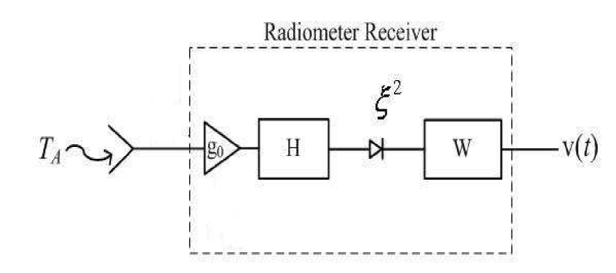
The schematic features the common components of most microwave radiometers. As the radiometer captures a signal (i.e. Brightness Temperature ), it couples the signal into a transmission line which then carries the signal to and from the various elements of the circuit. In Figure 2, a signal is introduced directly into the antenna, then it is mixed, amplified and filtered to produce the output signal . This filtering and amplification of the signal is carried out through the following components of the radiometer: an amplifier ; pre-detection filter ; a square law detector ; and a post-detection filter . The output of the radiometer is denoted as . See Ulaby et al. (1981) for a detailed discussion.
Racette and Lang (2005) state that at the core of every radiometer measurement is a calibrated receiver. Calibration is required due to the fact that the current electronic hardware is unable to maintain a stable input/output relationship. For space observing instruments, stable calibration without any drifts is a key to detect proper trends of climate (Imaoka et al. 2010). Due to problems such as amplifier gain instability and exterior temperature variations of critical components that may cause this relationship to drift over time (Bremer 1979). During the calibration process, the radiometer receiver measures the voltage output power , and its corresponding input temperature of a known reference. Two or more known reference temperatures are needed for calibration of a radiometer. Ulaby et al. (1981); Racette and Lang (2005) state that the relationship between the output, and the input, is approximately linear, and can be expressed as
where, is the estimated value of the brightness temperature, is the observed output voltage. Using this relationship, the output value, , is used to derive an estimate for the input, (Racette and Lang, 2005).
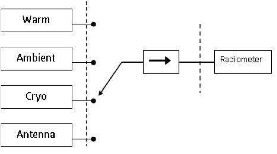
Traditional calibration methods use measurements taken from known calibration references, for example see Figure 3. Due to possible cost constraints it is common to use between two and five references. The reference temperatures are converted to their equivalent power measurement prior to the calibration algorithm. The radiometer outputs are observed when the radiometer measures the reference temperatures, giving an ordered calibration pair . The values are observed from the process of the electronics within the radiometer (see Figure 2) (Ulaby et al. 1981; Racette and Lang 2005). Through the process of calibration, the unknown brightness temperature is estimated by plugging its observed output into either Equation (3) or Equation (4).
It is of interest to develop a calibration approach that can detect gain abnormalities, and/or correct for slow drifts that affect the quality of the instrument measurements. To demonstrate the dynamic approach in terms of application appeal, the two dynamic methods were used to characterize a calibration target over time for a microwave radiometer. The data used for this example was collected during a calibration experiment that was conducted on the Millimeter-wave Imaging Radiometer (MIR) (Racette et al. 1995). The purpose of the experiment was to validate predictions of radiometer calibration.
The MIR was built with two internal blackbody references which will be used to observe a third stable temperature reference for an extended period of time. The third reference was a custom designed cryogenically cooled reference. Racette (2005) conducted the MIR experiment under two scenarios: the first experiment denoted as examined the calibration predictions when the unknown target is interior (i.e. interpolation) to the reference measurements; the second set of measurements (denoted as ) where taken when the unknown temperature to be estimated is outside (i.e. extrapolation) of the range of calibration references.
For demonstration purposes we will only consider the experiment, for details of the experiment see Racette (2005). For the run of the experiment, the reference temperatures are as follows:
-
1.
-
2.
with the unknown target temperature that must be estimated denoted as .
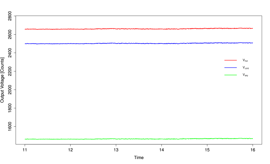
Each temperature measure has a corresponding observed time series of output measurements; , , and (see Figure 4). Therefore in this example we only consider a 2-point calibration set-up as we use and as the known reference standards and use to derive estimates of for the first 1000 time periods.
The results of the dynamic approaches: and , will be compared to the “inverse" calibration method (Krutchkoff 1967) implemented by Racette (2005). The method considered by Racette (2005) will be denoted as . As in practice, rarely does one know the value of the true temperature to be estimated so the aim of this example is to assess the contribution of the calibration approach to the variability in the measurement estimate. Racette (2005) analysis did not consider biases that may exist in calibration, continuing in the same spirit, the existence of biases will not be considered in the analysis. We will apply the , , and approaches to the data to estimate the temperature ; the standard deviation of the estimated time series is used as a measure of uncertainty including the contribution of the calibration algorithm.
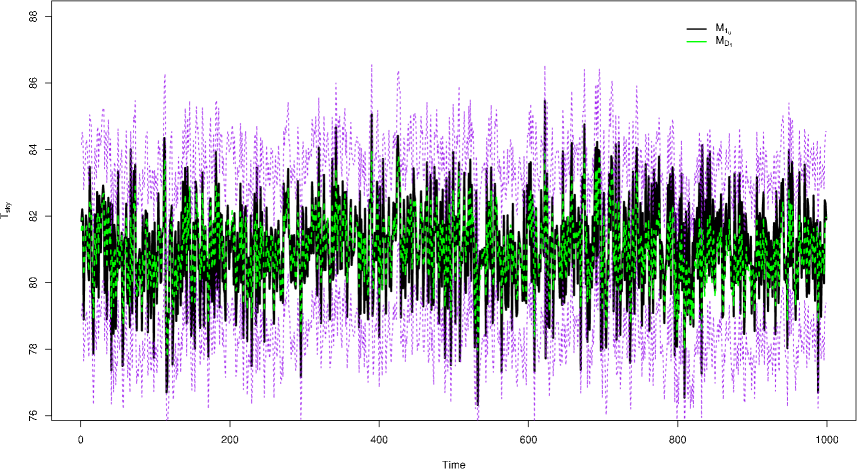
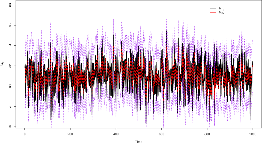
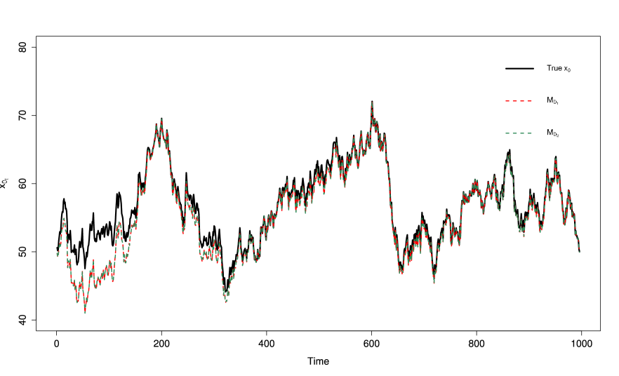
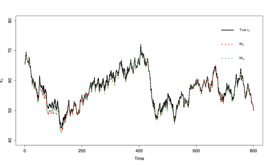
Figures 5 shows the time series of the temperature estimates for using Krutchkoff’s (1967) “inverse" approach and the dynamic approach . The standard deviations for the and approaches are and , respectfully. We see the dynamic model improves the estimation process over the static model by observing the corresponding standard deviation values. The dynamic model decreased the measurement uncertainty by roughly 33%. In Figure 6 the time series of the temperature estimates for using the “inverse" approach and the dynamic approach is given. The standard deviations for the and approaches are and . Again, the dynamic approach outperforms the static model . In this case, dynamic model decreased the measurement uncertainty by roughly 34%.
5. Discussion
Two new novel approaches to the statistical calibration problem have been presented in this paper. In was shown by the simulation results that the use of the dynamic approach has its benefits over the static methods. If the linear relationship in the first stage of calibration is known to be stable then the traditional methods should be used. The dynamic methods showed promise in the cases when the signal-to-noise ratio was high. There is also a computation expense to implementing the dynamic methods compared to the static methods, but in the sense of electronics these methods allow for near real time calibration and monitoring.
It is worth noting that the dynamic method shows possible deficiencies when the gain fluctuations is sinusoidal, referring to results in Table 1. In Figure 7 it is evident the largest source of the error is in the beginning of estimation process, roughly from to . The MSE values for the dynamic approaches; and were 4.41 and 4.40, respectively, which was vastly different than those reported for the static methods. This problem can be addressed by extending the burn-in period.
We increased the burn-in period to 200 which allowed the algorithm more time to learn and hence results in a lower MSE value. In Figure 8 we see that the estimates fit better to the true values of . The MSE decreased from 4.41 to 0.64 for and 0.63 for . The increased burn-in period improves the coverage probability but the interval width isn’t noticeably affected. The coverage probability increased from 0.628 to 0.722 for and from 0.829 to 0.964 for .
| 2 References-Sinusoidal Gain- wBurn In | |||
|---|---|---|---|
| Mean Squared Error | Coverage Probability | Interval Width | |
| 0.63553 | 0.72185 | 1.15722 | |
| 0.63333 | 0.96380 | 3.77191 | |
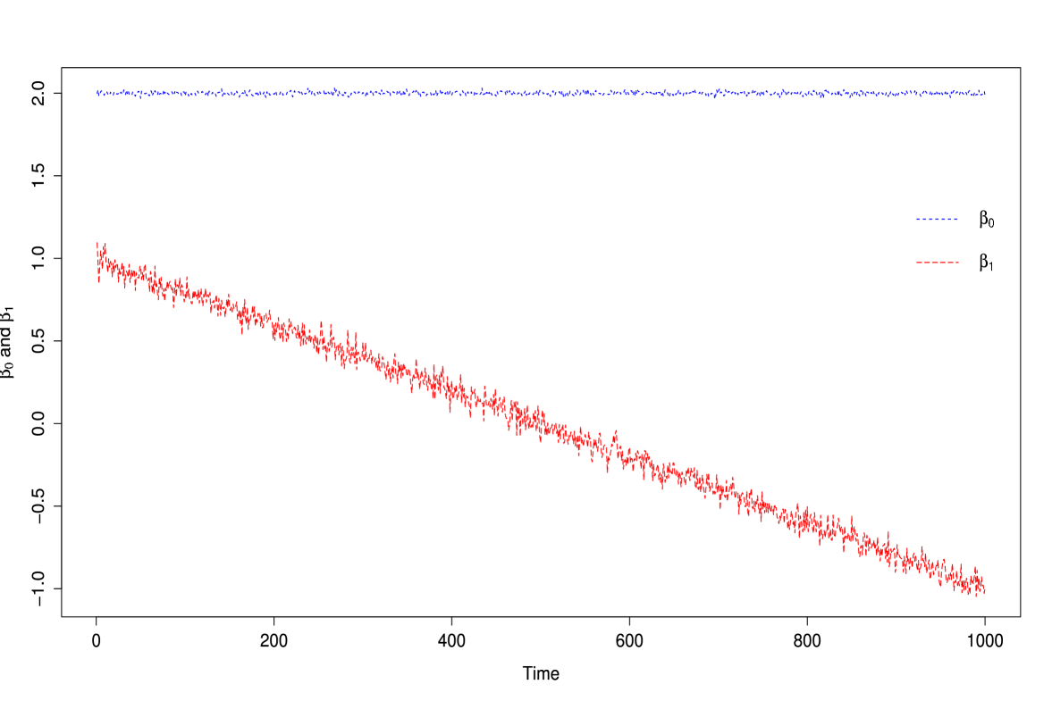

For completeness we consider the behavior of the method if crosses zero. It is absurd to believe that this would happen in practice because one would test the significance of (Myers 1990; Montgomery et al. 2012) for using any method where the possibility of dividing by zero could occur. We demonstrate this by generating data where for all time and drifts from 1 to -1 over time where (see Figure 9). Figure 10 shows the dynamic method is close to the true values of until get close to 0. Within the region where the slope crosses the the posterior estimates become unstable. Here we define unstable as meaning that we are within a region where there is division by zero. This instability is only present when , for every . As long as the dynamic method will perform well when estimating .
Some calibration problems are not linear or approximately linearly related in and . Future work is to investigate the dynamic calibration methods in the presence of nonlinearity. In such settings we may not have the ability to use only 2-points as references. Any approach will require more references in order to accurately capture the nonlinear behavior. Another area to be explored is using semiparametric regression which also allow for parameter variation across time and could be implemented in a near real time setting.
References
- [1] Albert, J. (2007). Bayesian Computation with R. New York: Springer.
- [2] Bernardo, J. M., and Smith, A. F. M. (1994). Bayesian Theory. John Wiley and Sons.
- [3] Bremer, J. C. (1979). Improvement of Scanning Radiometer Performance by Digital Reference Averaging. Instrumentation and Measurement, IEEE Transactions on 28.1: 46-54.
- [4] Brown, P. J. (1993). Measurement, Regression, and Calibration. Oxford University Press.
- [5] Draper, N. R., and Smith, H. (1998). Applied Regression Analysis. 3rd ed., John Wiley, Hoboken, N. J.
- [6] Eisenhart, C. (1939). The interpretation of certain regression methods and their use in biological and industrial research. Annals of Mathematical Statistics. 10, 162-186.
- [7] Eno, D. R. (1999). Noninformative Prior Bayesian Analysis for Statistical Calibration Problems. Doctoral dissertation, Virginia Polytechnic Institute and State University, Blacksburg, VA.
- [8] Eno, D. R., and Ye, K. (2000). Bayesian reference prior analysis for polynomial calibration models. Test, 9(1), 191-208.
- [9] Givens, G. H., and Hoeting, J. A. (2005). Computational Statistics. John Wiley and Sons.
- [10] Halperin, M. (1970). On Inverse Estimation in Linear Regression. Technometrics. 12, 727-736.
- [11] Hoadley, B. (1970). A Bayesian look at Inverse Linear Regression. Journal of the American Statistical Association. 65, 356-369.
- [12] Hunter, W., and Lamboy, W. (1981). A Bayesian Analysis of the Linear Calibration Problem. Technometrics. 23, 323-328.
- [13] Imaoka, K., Kachi, M., Kasahara, M., Ito, N., Nakagawa, K., and Oki, T. (2010). Instrument Performance and Calibration of AMSR-E and AMSR2. International Archives of the Photogrammetry, Remote Sensing and Special Information Science. 38(Part 8).
- [14] Krutchkoff, R. G. (1967). Classical and Inverse Regression Methods of Calibration. Technometrics. 9, 425-439.
- [15] Lwin, T. and Maritz, J. S. (1982). An Analysis of the Linear Calibration Controversy from the Perspective of Compound Estimation. Technometrics. 24, 235-242.
- [16] Montgomery, D.C., Peck, E.A. and Vining, G.G. (2012). Introduction to Linear Regression Analysis. Wiley.
- [17] Myers, R. H. (1990). Classical and Modern Regression With Applications. Duxbury/Thompson Learning.
- [18] Osborne, C. (1991). Statistical Calibration: A Review. International Statistical Review. 59, 309-336.
- [19] Ott, R.L. and Longnecker, M. (2009). An Introduction to Statistical Methods and Data Analysis. 6th ed., Brooks/Cole: Cengage Learning.
- [20] Özyurt, Ö., and Erar, A. (2003). Multivariate Calibration in Linear Regression and its Application. Hacettepe Journal of Mathematics and Statistics. 32, 53-63.
- [21] Petris, G., Petrone, S., and Campagnoli, P. (2009). Dynamic Linear Models with R. Springer-Verlag, New York.
- [22] R Development Core Team (2013). R: A Language and Environment for Statistical Computing. R Foundation for Statistical Computing, Vienna, Austria. ISBN 3-900051-07-0, URL: http://www.R-project.org.
- [23] Racette, P., Adler, R. F., Wang, J. R., Gasiewski, A. J., and Zacharias, D. S. (1996). An Airborne Millimeter-wave Imaging Radiometer for Cloud, Precipitation, and Atmospheric Water Vapor Studies. Journal of Atmospheric and Oceanic Technology, 13(3), 610-619.
- [24] Racette, P. E. (2005). Radiometer Design Analysis Based Upon Measurement Uncertainty (Unpublished doctoral dissertation). The George Washington University, Washington D.C.
- [25] Racette, P. E., and Lang, R. H. (2005). Radiometer Design Analysis Based Upon Measurement Uncertainty. Radio Science. 40(5).
- [26] Ulaby, F. T., Moore, R. K., and Fung, A. K. (1981). Microwave Remote Sensing:Active and Passive, Vol. I: Fundamentals and Radiometry. Addison-Wesley, Advanced Book Program, Reading, Massachusetts.
- [27] West, M., Harrison, P. J., and Migon, H. S. (1985). Dynamic generalized linear models and Bayesian forecasting. Journal of the American Statistical Association, 80(389), 73-83.
- [28] West, M. and P.J. Harrison (1997). Bayesian Forecasting and Dynamic Linear Models, 2nd Edition. Springer-Verlag, New York.