A fast compact difference scheme with unequal time-steps for the tempered time-fractional Black-Scholes model

Jinfeng Zhou¹¹1School of Mathematics, Southwestern University of Finance and Economics, Chengdu, Sichuan 611130, P.R. China. E-mail: 2207441009@qq.com; guxianming@live.cn, guxm@swufe.edu.cn (corresponding author), Xian-Ming Gu^§,¹¹1School of Mathematics, Southwestern University of Finance and Economics, Chengdu, Sichuan 611130, P.R. China. E-mail: 2207441009@qq.com; guxianming@live.cn, guxm@swufe.edu.cn (corresponding author), Yong-Liang Zhao²²2School of Mathematical Sciences, Sichuan Normal University, Chengdu, Sichuan 610068, P.R. China. E-mail: ylzhaofde@sina.com, Hu Li³³3School of Mathematics, Chengdu Normal University, Chengdu, Sichuan 611130, P.R. China. E-mail: lihu_0826@163.com

Abstract

The Black-Scholes (B-S) equation has been recently extended as a kind of tempered time-fractional B-S equations, which becomes an interesting mathematical model in option pricing. In this study, we provide a fast numerical method to approximate the solution of the tempered time-fractional B-S model. To achieve high-order accuracy in space and overcome the weak initial singularity of exact solution, we combine the compact difference operator with L1-type approximation under nonuniform time steps to yield the numerical scheme. The convergence of the proposed difference scheme is proved to be unconditionally stable. Moreover, the kernel function in the tempered Caputo fractional derivative is approximated by sum-of-exponentials, which leads to a fast unconditionally stable compact difference method that reduces the computational cost. Finally, numerical results demonstrate the effectiveness of the proposed methods.

Keywords: Tempered time-fractional B-S model; nonuniform time steps; exponential transformation; compact difference scheme; weak regularity.

AMS subject classifications: 65M06, 65M50, 26A33, 91G20.

1 Introduction

The Black-Scholes (B-S) model is an important method of option pricing because of its clever combination of option pricing, random fluctuation of underlying asset price and risk-free interest rate [1]. However, the classic B-S model was put forward by Black and Scholes under a series of assumptions [2]. Through observation and research on the stock market, many scholars found that the essential characteristics and state of the capital market are random fluctuations, which are not completely consistent with these assumptions of the traditional B-S option pricing model. The pricing of the model is different from the actual market price. Therefore, in order to extend the application of B-S equation from the ideal state of stock price to a more realistic state, many scholars have done a lot of work, such as B-S model with transaction cost [3], stochastic interest rate model [4], jump-diffusion model [5], etc.

Besides, in order to make Brownian motion reflect more properties such as autocorrelation, long-term memory and incremental correlation, some other scholars began to consider modifying the original partial differential equation (DE) of Brownian motion which leads to new option pricing models which are more suitable for the actual financial market. With the discovery of the fractal structure of DEs in the financial field, more and more attention has been paid to such fractional DEs in this field. In 2000, Wyss [6] first applied the idea of fractal to the financial field and deduced the time-fractional B-S (TFBS) option pricing model. Later, Jumariel [7] use the fractional Taylor formula to deduce and demonstrate the TFBS option pricing formula, Cartea [8] propose to model stock price tick-by-tick data via a non-explosive marked point process where the model equation satisfied by the value of European-style derivatives contains a Caputo fractional derivative in time-to-maturity. Liang et al. [9] proposed a special TFBS equation based on the real market option price analysis in a fractional transfer system. Magdziarz [10] consider a generalization of this model, which is based on a subdiffusive geometric Brownian motion and captures the subdiffusive characteristics of financial markets. There are also other TFBS models available at [11, 12, 3].

With the development of TFBS model, there is a growing concern on its solution which is hard to be solved in the analytical manner [9, 11, 13]. Thus it is necessary to study efficient numerical methods for such models. Krzyz̀anowskia et al. [14] present the weighted finite difference method to solve the subdiffusive B-S model numerically and prove its convergence. In [15], the numerical solution of the TFBS model governing European options is obtained by using the L1 approximation of Caputo fractional derivatives, which can achieve ( $2-\alpha$ )-order accuracy in time and second-order accuracy in space. Tian et al. [16] proposed three compact finite difference schemes for the TFBS model governing European option pricing where the time fractional derivative is approximated by L1 formula, L2-1_σ formula and L1-2 formula, then convergence orders of these three compact difference schemes are fourth-order in space and $(2-\alpha)$ -, 2-, and $(3-\alpha)$ -order in time, respectively. Staelen and Hendy [2] studied an implicit numerical scheme with a temporal accuracy of ( $2-\alpha$ )-order and the spatial accuracy of fourth-order by using the Fourier analysis method. In addition, some other related numerical methods based on different spatial discrezations for the TFBS model can be found in [17, 18, 19, 20, 22, 21, 23, 24, 25].

It is worth noting that the above numerical methods can reach the theoretical convergence order with the assumption that the exact solution of TFBS model is sufficiently smooth in the time variable. But in fact, exact solutions of time-fractional partial DEs always enjoy the weak singularity near the initial time, this fact makes most of the above numerical methods fail to achieve the optimal order convergence [27, 26]. In order to overcome the weakly initial singularity of exact solution, numerical methods with nonuniform time steps introduced in [26, 28, 29] have been considered to solve the model problem; see e.g., [30, 31] for details. In order to overcome the difficulty of initial layer, She et al. [32] present modified L1 time discretization is presented based on a change of variable for solving the TFBS model. However all the above numerical methods need huge storage and computational cost due to the nonlocal time fractional derivative. In order to reduce the computational cost, Song and Lyu [33] use the fast sum-of-exponentials (SOE) approximation of of Caputo fractional derivative [34, 29] to present a fast numerical method for TFBS equations, the fast algorithm keeps the convergence of second-order accuracy in time and fourth-order accuracy in space. Moreover, it reduces the computational complexity significantly. The stability of their proposed schemes is established base on the analysis framework developed in [35].

When we consider the option pricing in such a stagnated market, the tempered TFBS model does better in estimating the fair price than the classic B-S model, Krzyzanowskia and Magdziarza [36] proposed the tempered subdiffusive B-S model assumed that the underlying asset is driven by $\alpha$ -stable $\lambda$ -tempered inverse subordinator [38, 37]. In this paper, we are interested in such a tempered TFBS model governing European options:

\begin{cases}\frac{\partial^{\alpha,\lambda}C(S,t)}{\partial t^{\alpha,\lambda}}+\frac{1}{2}\sigma^{2}S^{2}\frac{\partial^{2}C(S,t)}{\partial S^{2}}+\hat{r}S\frac{\partial C(S,t)}{\partial S}-rC(S,t)=0,&(S,t)\in(0,+\infty)\times[0,T),\\ C(S,T)=\mu(S),&S\in(0,+\infty),\\ C(0,t)=\phi(t),\quad C(+\infty,t)=\varphi(t),&t\in[0,T),\end{cases}

(1.1)

where $\alpha\in(0,1)$ and $\lambda\geq 0$ , $T$ is the expiry time, $\hat{r}=r-D$ ( $r>0$ and $D\geq 0$ are the risk-free rate and the dividend yield, respectively) and $\sigma>0$ is the volatility of the returns from the holding stock price $S$ . Here the terminal condition is typically chosen as $\mu(S)$ for the payoff of the option. The fractional derivative operator in Eq. (1.1) is a modified right Riemann-Liouville tempered fractional derivative defined as

\frac{\partial^{\alpha,\lambda}C(S,t)}{\partial t^{\alpha,\lambda}}=\frac{e^{-\lambda(T-t)}}{\Gamma(1-\alpha)}\frac{\partial}{\partial t}\int^{T}_{t}\frac{e^{-\lambda(\xi-T)}C(S,\xi)-C(S,T)}{(\xi-t)^{\alpha}}d\xi,

(1.2)

where $\alpha=1$ and $\lambda=0$ , the model (1.1) collapses to the classical B-S model.

Let $\tau=T-t$ , $e^{x}=S$ and $U(x,\tau)=C(S,t)$ , some tedious but simple calculations yield

\begin{split}-\frac{\partial^{\alpha,\lambda}C(S,t)}{\partial t^{\alpha,\lambda}}&=\frac{e^{-\lambda\tau}}{\Gamma(1-\alpha)}\frac{\partial}{\partial\tau}\int^{\tau}_{0}\frac{e^{\lambda\eta}C(S,T-\eta)-C(S,T)}{(\tau-\eta)^{\alpha}}d\eta\\ &=\frac{e^{-\lambda\tau}}{\Gamma(1-\alpha)}\frac{\partial}{\partial\tau}\int^{\tau}_{0}\frac{e^{\lambda\eta}U(x,\eta)-U(x,0)}{(\tau-\eta)^{\alpha}}d\eta\\ &=\frac{e^{-\lambda\tau}}{\Gamma(1-\alpha)}\int^{\tau}_{0}\frac{1}{(\tau-\eta)^{\alpha}}\cdot\frac{\partial[e^{\lambda\eta}U(x,\eta)]}{\partial\eta}d\eta\\ &\triangleq{}^{C}_{0}\mathbb{D}^{\alpha,\lambda}_{\tau}U(x,\tau),\end{split}

(1.3)

where ${}^{C}_{0}\mathbb{D}^{\alpha,\lambda}_{\tau}$ is the tempered Caputo fractional derivative (tCFD) [39, Eq. (3)]. To solve the above model numerically, it always truncates the original infinite $x$ -domain $\in\mathbb{R}$ to a finite domain $\Omega\cap\partial\Omega=[x_{l},x_{r}]$ , then the model (1.1) can be eventually rewritten as

\begin{cases}{}^{C}_{0}\mathbb{D}^{\alpha,\lambda}_{\tau}U(x,\tau)=\frac{1}{2}\sigma^{2}\frac{\partial^{2}U(x,\tau)}{\partial x^{2}}+c\frac{\partial U(x,\tau)}{\partial x}-rU(x,\tau)+f(x,\tau),&(x,\tau)\in\Omega\times(0,T],\\ U(x,0)=\zeta(x),&x\in\Omega,\\ U(x_{l},\tau)=\phi(\tau),\quad U(x_{r},\tau)=\varphi(\tau),&\tau\in(0,T],\end{cases}\vspace{-2mm}

(1.4)

where $c=\hat{r}-\frac{1}{2}\sigma^{2}$ , $\kappa(x)=\mu(e^{x})$ and a source term $f(x,\tau)$ is just added for the purposes of validation in Section 4 without loss of generality. Meanwhile, the initial condition is chosen as $\zeta(x)=\max(K-e^{x},0)$ (which is only continuous) as suggested by the model (1.1). In addition, the above equation (1.4) can be viewed a special case of the tempered time-fractional advection-diffusion-reaction equations [40].

In fact, the paper [36] presents a finite difference method that has the $(2-\alpha)$ - and 2-order of accuracy with respects to time and space respectively to the option pricing in the model (1.1). However, such a study seems to be less efficient because it overlooks two numerical difficulties of the tempered TFBS model, i.e., the nonlocal time tCFD and the weakly initial singularity of the exact solution. In order to remedy such numerical difficulties, we first transform the model (1.4) into a tempered time-fractional diffusion-reaction (tTFDR) equation with homogeneous boundary conditions (BCs), which holds the same solution. Then the regularity of exact solution of the transformed tTFDRE equation is investigated by the method of variable separation that is different from the idea we extend introduced in [41]. Moreover, an implicit difference method with the compact difference operator in space and the graded L1 formula in time will be derived for such a transformed tTFDR equation with homogeneous BCs. To reduce the computational cost caused by the nonlocal tCFD, the fast SOE approximation [34, 29] is extended to reconstruct a fast difference method for the transformed tTFDR equation. Meanwhile, the proposed schemes are proved to be unconditional stable and convergent with the $(2-\alpha)$ - and 4-order of accuracy with respects to time and space, respectively. Finally, we report some numerical experiments to examine the feasibility of the proposed methods.

The rest of the paper is organized as follows. In Section 2, the nonuniform temporal discretization is used to set up a compact difference scheme for the equivalent tTFDR equation. Moreover, the unconditional stability and convergence of $\min\left\{\gamma\alpha,2-\alpha\right\}$ -order in time (where the mesh grading index $\gamma\geq 1$ is chosen by the user) and fourth-order in space of the proposed scheme are displayed by mathematical introductions. In Section 3, we establish a fast compact difference scheme that reduces the computational cost and then state the convergence for solving the equivalent tTFDR equation. Numerical examples are provided in Section 4 to show the theoretical statements. A brief conclusion is followed in Section 5.

2 Construction of the compact difference scheme

In this section. We first establish a direct finite difference scheme for solving the equivalent tTFDR equation. Since it is well-known that the exact solution of Eq. (1.4) always has the weak singularity at the initial time (see Appendix A for details), i.e., the solution will be non-smooth enough near the initial time, then the classical L1 scheme cannot achieve the optimal convergence order of $(2-\alpha)$ . Alternatively, the non-uniform temporal discretization is proved to be a reliable numerical technique for solving the equivalent tTFDR equation.

2.1 The equivalent reformulation of tTFDR equations

In order to simplify the derivation of the high-order spatial discrezation for the model (1.4), we first denote $v(x,\tau):=k(x)[U(x,\tau)-z(x,\tau)]$ , where

z(x,\tau):=\frac{\varphi(\tau)-\phi(\tau)}{x_{r}-x_{l}}(x-x_{l})+\phi(\tau)\quad{\rm and}\quad k(x)=\exp\Big{(}\frac{c(x-x_{l})}{\sigma^{2}}\Big{)},

(2.1)

then it is not hard to note that the problem (2.2) is equivalent to the next equations with homogeneous BCs:

\begin{cases}{}^{C}_{0}\mathbb{D}^{\alpha,\lambda}_{\tau}v(x,\tau)=\frac{1}{2}\sigma^{2}\frac{\partial^{2}v(x,\tau)}{\partial x^{2}}-qv(x,\tau)+g(x,\tau),&(x,\tau)\in\Omega\times(0,T],\\ v(x,0)=\sigma(x),&x\in\Omega,\\ v(x,\tau)=0,&(x,\tau)\in\partial\Omega\times(0,T],\end{cases}\vspace{-1.5mm}

(2.2)

where $q=\frac{c^{2}}{2\sigma^{2}}+r>0$ , $\sigma(x)=k(x)[\zeta(x)-z(x,0)]$ and $g(x,\tau)=k(x)[f(x,\tau)+cz_{x}(x,\tau)-rz(x,\tau)-{}^{C}_{0}\mathbb{D}^{\alpha,\lambda}_{\tau}z(x,\tau)]$ ¹¹1Due to two known functions $\phi(\tau)$ and $\varphi(\tau)$ , it is easy to compute the term ${}^{C}_{0}\mathbb{D}^{\alpha,\lambda}_{\tau}z(x,\tau)$ in the analytical (or numerical) manner. and it is clear that $U(x,\tau)$ is a solution of (1.4) if and only if $v(x,\tau)$ is a solution of (2.2); refer to [42, 16, 33] for details. Therefore, in the following, our proposed finite difference methods for the problem (1.4) are based on the equivalent form (2.2).

2.2 Discretization in time on non-uniform steps

For nonuniform time levels $\tau_{n}=T\left(\frac{n}{M}\right)^{\gamma}$ , the $n$ -th time step size is set as $\Delta\tau_{n}:=\tau_{n}-\tau_{n-1}$ with $n=0,1\ldots,M$ , the spatial grid nodes $x_{i}=x_{l}+ih,i=0,1,\cdots,N$ , where $h=(x_{r}-x_{l})/N$ are space grid size and $M,N\in\mathbb{N}^{+}$ respectively. Since the grid function $\{v_{i}|0\leq i\leq N\}$ , then we define the following difference operators:

\delta_{x}v_{i-1/2}=\frac{v_{i}-v_{i-1}}{h},~{}~{}\delta^{2}_{x}v_{i}=\frac{v_{i+1}-2v_{i}+v_{i-1}}{h^{2}},~{}~{}\mathcal{H}_{x}v_{i}=\begin{cases}\left(1+\frac{h^{2}}{12}\delta^{2}_{x}\right)v_{i},&1\leq i\leq N-1,\\ v_{i},&i=0,~{}N,\end{cases}\vspace{-2mm}

Let $\Pi_{1,n}u$ denote the linear interpolation of a function $u(\tau)$ with respect to the nodes $\tau_{n-1}$ and $\tau_{n}$ , then it is easy to find that

(\Pi_{1,n}u)^{\prime}(\tau)=\frac{u(\tau_{n})-u(\tau_{n-1})}{\Delta\tau_{n}}:=\frac{\nabla_{\tau}u^{n}}{\Delta\tau_{n}},

At this stage, we recall $u(\tau_{n})=e^{\lambda\tau_{n}}v(\tau_{n})$ and extend the L1 formula on graded meshes [26] for tCFD at the time point $\tau_{n}$ :

\begin{split}{}^{C}_{0}\mathbb{D}^{\alpha,\lambda}_{\tau}v(\tau_{n})&=\frac{e^{-\lambda\tau_{n}}}{\Gamma(1-\alpha)}\sum^{n}_{k=1}\int^{\tau_{k}}_{\tau_{k-1}}(\tau_{k}-\eta)^{-\alpha}(\Pi_{1,k}u)^{\prime}(\eta)d\eta+\mathcal{R}^{n}\\ &=\frac{e^{-\lambda\tau_{n}}}{\Gamma(1-\alpha)}\sum^{n}_{k=1}a_{k}^{(n,\alpha)}(u^{k}-u^{k-1})+\mathcal{R}^{n}\left(:=e^{-\lambda\tau_{n}}\cdot\mathcal{D}^{\alpha}_{\tau}u(\tau_{n})\right)\\ &=\frac{1}{\Gamma(1-\alpha)}\Bigg{[}a^{(n,\alpha)}_{n}v(\tau_{n})-\sum^{n-1}_{k=1}(a^{(n,\alpha)}_{k+1}-a_{k}^{(n,\alpha)})e^{\lambda(\tau_{k}-\tau_{n})}v(\tau_{k})~{}-\\ &\quad~{}a_{1}^{(n,\alpha)}e^{\lambda(\tau_{0}-\tau_{n})}v(\tau_{0})\Bigg{]}+\mathcal{R}^{n}\\ &:=\mathcal{D}^{\alpha,\lambda}_{\tau}v(\tau_{n})+\mathcal{R}^{n},\end{split}

(2.3)

where $\mathcal{R}^{n}:={}^{C}_{0}\mathbb{D}^{\alpha,\lambda}_{\tau}v(\tau)\mid_{\tau=\tau_{n}}-\mathcal{D}^{\alpha,\lambda}_{\tau}v(\tau_{n})$ is the truncation error and

\begin{split}a_{k}^{(n,\alpha)}&=\frac{1}{\Delta\tau_{k}}\int_{\tau_{k-1}}^{\tau_{k}}\frac{\mathrm{d}s}{(\tau_{n}-s)^{\alpha}}\\ &=\frac{(\tau_{n}-\tau_{k-1})^{1-\alpha}-(\tau_{n}-\tau_{k})^{1-\alpha}}{(1-\alpha)\Delta\tau_{k}},\quad k=1,2,\cdots,n.\end{split}

(2.4)

Here the above formula (2.3) is named after the nonuniform tempered L1 formula. Obviously, if $\lambda\equiv 0$ , the approximate formula (2.3) reduces to the nonuniform L1 formula for approximating the Caputo fractional derivative [29].

Remark 2.1.

Although the exact integration is used to evaluate the coefficients $a^{(n,\alpha)}_{k}$ in Eq. (2.4), when the fractional order $\alpha$ is small and the grading index $\gamma$ is large, then $(\tau_{n}-\tau_{k})^{1-\alpha}$ is very close to $(\tau_{n}-\tau_{k-1})^{1-\alpha}$ and thus the round-off error of this subtraction in Eq. (2.4) will be remarkable in the numerical implementation and even it cannot yield some acceptable numerical results²²2See some related experimental results in our arXiv preprint https://arxiv.org/abs/2303.10592v2.. In order to overcome such an issue, we first introduce some notations and follow the idea in [43, Section 4] to derive a computational stable implementation:

d_{k}(\tau)=\tau-\tau_{k},\quad\kappa_{k}(\tau)=\ln\Bigg{(}\frac{d_{k}(\tau)}{d_{k-1}(\tau)}\Bigg{)}={\tt log1p}\Bigg{(}-\frac{\Delta\tau_{k}}{\tau-\tau_{k-1}}\Bigg{)}.

(2.5)

Now, according to Eq. (2.4), we have $a^{(n,\alpha)}_{n}=\frac{1}{(1-\alpha)(\Delta\tau_{n})^{\alpha}}$ and

\begin{split}a^{(n,\alpha)}_{k}&=\frac{-[d_{k-1}(\tau_{n})]^{1-\alpha}}{(1-\alpha)\Delta\tau_{k}}\Bigg{[}\Bigg{(}\frac{d_{k}(\tau_{n})}{d_{k-1}(\tau_{n})}\Bigg{)}^{1-\alpha}-1\Bigg{]}\\ &=\frac{-[d_{k-1}(\tau_{n})]^{1-\alpha}}{(1-\alpha)\Delta\tau_{k}}{\tt expm1}((1-\alpha)\kappa_{k}(\tau_{n})),\quad k=1,2,\cdots,n-1,\\ \end{split}

(2.6)

where “expm1” and “log1p” are two built-in functions in MATLAB. After such a new formula for $a^{(n,\alpha)}_{k}$ is utilized in the nonuniform tempered L1 formula (2.3), we observed stable performance of the above reformulation in all our experiments.

In what follows, $C$ and $c_{j}$ are constants, which depend on the problem but not on the mesh parameters. Moreover, we can give the following properties of the coefficients $a^{(\alpha,n)}_{k}$ :

Lemma 2.1.

([29]) For $\alpha\in(0,1)$ and $\{a_{k}^{(n,\alpha)}|1\leqslant n\leqslant M\}~{}$ defined in Eq. (2.4), it holds

	$\displaystyle 0<a_{1}^{(n,\alpha)}<a_{2}^{(n,\alpha)}<\cdots<a_{n}^{(n,\alpha)},~{}~{}n=1,2,\cdots,M,$		(2.7)
	$\displaystyle a_{1}^{(1,\alpha)}>a_{1}^{(2,\alpha)}>\cdots>a_{1}^{(N,\alpha)}\geq T^{-\alpha}.$		(2.8)

There exists a constant $c_{1}$ such that $a_{n}^{(n,\alpha)}-a_{n-1}^{(n,\alpha)}\geq c_{1}M^{\alpha}$ with $n=2,3,\cdots,M$ .

The error of such an approximation (2.3) can be evaluated.

Lemma 2.2.

Suppose $|v^{\prime\prime}(\tau)|\leqslant c_{0}\tau^{\alpha-2},~{}0<\tau\leqslant T.$ Then there exists a constant $C$ such that

\left|\mathcal{R}^{n}\right|=\left|{}_{0}^{C}\mathbb{D}^{\alpha,\lambda}_{\tau}v(\tau_{n})-\mathcal{D}^{\alpha,\lambda}_{\tau}v(\tau_{n})\right|\leq Cn^{-\min{\{\gamma(1+\alpha),2-\alpha\}}},\quad n=1,2,\ldots,M.

(2.9)

Proof.

We still recall $u(\tau)=e^{\lambda\tau}v(\tau)$ . If $|v^{\prime\prime}(\tau)|<c_{0}\tau^{\alpha-2}$ , then it is not hard to verify that $|u^{\prime\prime}(\tau)|<\tilde{c}_{0}\tau^{\alpha-2}$ . Moreover,

\vspace{-2mm}\begin{split}\left|{}_{0}^{C}\mathbb{D}^{\alpha,\lambda}_{\tau}v(\tau_{n})-\mathcal{D}^{\alpha,\lambda}_{\tau}v(\tau_{n})\right|&=\Bigg{|}\Big{[}e^{-\lambda\tau}\cdot{}_{0}^{C}\mathbb{D}^{\alpha}_{\tau}u(\tau)\Big{]}\Big{|}_{\tau=\tau_{n}}-e^{-\lambda\tau_{n}}\cdot\mathcal{D}^{\alpha}_{\tau}u(\tau_{n})\Bigg{|}\\ &\leq\left|e^{-\lambda\tau_{n}}\right|\cdot\Big{|}{}^{C}_{0}\mathbb{D}^{\alpha}_{\tau}u(\tau_{n})-\mathcal{D}^{\alpha}_{\tau}u(\tau_{n})\Big{|}\\ &\leq\Big{|}{}^{C}_{0}\mathbb{D}^{\alpha}_{\tau}u(\tau_{n})-\mathcal{D}^{\alpha}_{\tau}u(\tau_{n})\Big{|},\end{split}

(2.10)

where ${}^{C}_{0}\mathbb{D}^{\alpha}_{\tau}u(\tau)$ is the $\alpha$ -order Caputo derivative of a function $u(\tau)$ , cf. [29, Eq. (1.4)].

Furthermore, with the help of the estimate in [29, Lemma 2.1 and Eq. (2.3)], it gives

\Big{|}{}^{C}_{0}\mathbb{D}^{\alpha}_{\tau}u(\tau_{n})-\mathcal{D}^{\alpha}_{\tau}u(\tau_{n})\Big{|}\leq Cn^{-\min\{\gamma(1+\alpha),2-\alpha\}},\quad n=1,2,\ldots,N,

(2.11)

and insert it into the inequality (2.10) to obtain the desired error estimate (2.9). ∎

Next, we consider Eq. (2.2) at the point $(x,\tau)=(x_{i},\tau_{n})$ , then it follows that

{}^{C}_{0}\mathbb{D}^{\alpha,\lambda}_{\tau}v(x_{i},\tau_{n})=\frac{1}{2}\sigma^{2}\frac{\partial^{2}v(x_{i},\tau_{n})}{\partial x^{2}}-qv(x_{i},\tau_{n})+g(x_{i},\tau_{n}),

(2.12)

Let $V$ be a grid function defined by $V^{n}_{i}:=v(x_{i},t_{n})$ with $0\leq i\leq N,~{}0\leq n\leq M$ . Using this notation and recalling relations (2.3)-(2.4) along with Lemma 2.9, we can write Eq. (2.2) at the grid points $(x_{i},t_{n})$ as follows

\begin{cases}\mathcal{H}_{x}\Big{(}\mathcal{D}^{\alpha,\lambda}_{\tau}V^{n}_{i}\Big{)}=\frac{1}{2}\sigma^{2}\delta^{2}_{x}V^{n}_{i}-q\mathcal{H}_{x}V^{n}_{i}+\mathcal{H}_{x}g^{n}_{i}+\mathcal{R}^{n}_{i},&1\leq i\leq N-1,~{}1\leq n\leq M,\\ V^{0}_{i}=\sigma(x_{i}),&1\leq i\leq N-1,\\ V^{n}_{0}=V^{n}_{N}=0,&0\leq n\leq M,\end{cases}

(2.13)

where the terms $\{\mathcal{R}^{n}_{i}\}$ are small and satisfy the inequality

\left|\mathcal{R}^{n}_{i}\right|\leq c_{2}\big{(}n^{-\min\{\gamma(1+\alpha),2-\alpha\}}+h^{4}\big{)},\quad 1\leq i\leq N-1,~{}1\leq n\leq M.

Now, we omit the small error items and arrive at the following difference schemes

\begin{cases}\mathcal{H}_{x}\Big{(}\mathcal{D}^{\alpha,\lambda}_{\tau}v^{n}_{i}\Big{)}=\frac{1}{2}\sigma^{2}\delta^{2}_{x}v^{n}_{i}-q\mathcal{H}_{x}v^{n}_{i}+\mathcal{H}_{x}g^{n}_{i},&1\leq i\leq N-1,~{}1\leq n\leq M,\\ v^{0}_{i}=\sigma(x_{i}),&1\leq i\leq N-1,\\ v^{n}_{0}=v^{n}_{N}=0,&0\leq n\leq M,\end{cases}

(2.14)

which is called the direct scheme (DS).

2.3 Stability and convergence of the compact difference scheme

In this subsection, we present the stability and convergence analysis of the direct difference scheme (2.14).

Theorem 2.3.

Suppose $\{v_{i}^{n}\,|\,0\leqslant i\leqslant N,~{}0\leq n\leq M\}$ is the solution of the difference scheme (2.14). Then, it holds

\displaystyle\|v^{k}\|_{\infty}\leqslant\|v^{0}\|_{\infty}+\Gamma(1-\alpha)\max\limits_{1\leq m\leq k}\frac{\|g^{m}\|_{\infty}}{a_{1}^{(m,\alpha)}},\quad k=1,2,\cdots,M,

(2.15)

where $\|g^{m}\|_{\infty}=\max\limits_{1\leq i\leq N-1}|g_{i}^{m}|$ .

Proof.

Let $i_{0}~{}(1\leq i_{0}\leq N-1)$ be an index such that $|v_{i_{0}}^{n}|=\|v^{n}\|_{\infty}.$ Rewriting the first equality of Eq. (2.14) in the form

\begin{split}\Bigg{[}\frac{1}{\Gamma(1-\alpha)}a_{n}^{(n,\alpha)}+q\Bigg{]}\mathcal{H}_{x}v_{i}^{n}+\frac{\sigma^{2}}{h^{2}}v_{i}^{n}&=\frac{\sigma^{2}}{2h^{2}}(v_{i-1}^{n}+v_{i+1}^{n})+\frac{1}{\Gamma(1-\alpha)}\Bigg{[}\sum_{k=1}^{n-1}e^{-\lambda(\tau_{n}-\tau_{k})}\cdot\\ &~{}~{}~{}~{}(a_{k+1}^{(n,\alpha)}-a_{k}^{(n,\alpha)})\mathcal{H}_{x}v_{i}^{k}+e^{-\lambda(\tau_{n}-\tau_{0})}a_{1}^{(n,\alpha)}\mathcal{H}_{x}v_{i}^{0}\Bigg{]}\\ &~{}~{}~{}+\mathcal{H}_{x}g_{i}^{n},\quad 1\leqslant i\leqslant N-1,\quad 1\leqslant n\leqslant M,\end{split}

(2.16)

we set $i=i_{0}$ in Eq. (2.16) and take the absolute value on the both sides of the equation obtained so that

\begin{split}\Big{[}\frac{1}{\Gamma(1-\alpha)}a_{n}^{(n,\alpha)}+q\Big{]}\|v^{n}\|_{\infty}+\frac{\sigma^{2}}{h^{2}}\|v^{n}\|_{\infty}&\leqslant\frac{\sigma^{2}}{h^{2}}\|v^{n}\|_{\infty}+\frac{1}{\Gamma(1-\alpha)}\Big{[}\sum_{k=1}^{n-1}(a_{k+1}^{(n,\alpha)}-a_{k}^{(n,\alpha)})\|v^{k}\|_{\infty}\\ &~{}~{}~{}+a_{1}^{(n,\alpha)}\|v^{0}\|_{\infty}\Big{]}+\|g^{n}\|_{\infty},\quad 1\leqslant n\leqslant M\end{split}

with the help of $\|v^{n}\|_{\infty}=\|\mathcal{H}_{x}v^{n}\|_{\infty}$ . This inequality can be rearranged and written as follows,

\begin{split}a_{n}^{(n,\alpha)}\|v^{n}\|_{\infty}&\leqslant\sum_{k=1}^{n-1}(a_{k+1}^{(n,\alpha)}-a_{k}^{(n,\alpha)})\|v^{k}\|_{\infty}+a_{1}^{(n,\alpha)}\Big{(}\|v^{0}\|_{\infty}\\ &~{}~{}~{}+\frac{\Gamma(1-\alpha)}{a_{1}^{(n,\alpha)}}\|g^{n}\|_{\infty}\Big{)},\quad 1\leqslant n\leqslant M.\end{split}

(2.17)

Next, we apply mathematical induction to prove (3.16) is valid. In fact, setting $n=1$ in (2.17) and noticing $a_{1}^{(1,\alpha)}>0,$ we obtain

\|v^{1}\|_{\infty}\leqslant\|v^{0}\|_{\infty}+\frac{\Gamma(1-\alpha)}{a_{1}^{(1,\alpha)}}\|g^{1}\|_{\infty}.

Thus (3.16) is valid for $k=1.$ Assume that the inequality (3.16) holds for $1\leqslant k\leqslant n-1$ , i.e.,

\displaystyle\|v^{k}\|_{\infty}\leqslant\|v^{0}\|_{\infty}+\Gamma(1-\alpha)\max_{1\leq m\leq k}\frac{\|g^{m}\|_{\infty}}{a_{1}^{(m,\alpha)}},\quad k=1,2,\cdots,n-1.

Then, from (2.17), we have

$\displaystyle a_{n}^{(n,\alpha)}\\|v^{n}\\|_{\infty}$	$\displaystyle\leqslant\sum_{k=1}^{n-1}(a_{k+1}^{(n,\alpha)}-a_{k}^{(n,\alpha)})\big{(}\\|v^{0}\\|_{\infty}+\Gamma(1-\alpha)\max_{1\leqslant m\leqslant k}\frac{\\|g^{m}\\|_{\infty}}{a_{1}^{(m,\alpha)}}\big{)}+a_{1}^{(n,\alpha)}\big{[}\\|v^{0}\\|_{\infty}$
	$\displaystyle+\Gamma(1-\alpha)\frac{\\|g^{n}\\|_{\infty}}{a_{1}^{(n,\alpha)}}\big{]}$
	$\displaystyle\leqslant\big{[}\sum_{k=1}^{n-1}(a_{k+1}^{(n,\alpha)}-a_{k}^{(n,\alpha)})+a_{1}^{(n,\alpha)}\big{]}\big{(}\\|v^{0}\\|_{\infty}+\Gamma(1-\alpha)\max_{1\leq m\leq n}\frac{\\|g^{m}\\|_{\infty}}{a_{1}^{(m,\alpha)}}\big{)}$
	$\displaystyle\leqslant a_{n}^{(n,\alpha)}[\\|v^{0}\\|_{\infty}+\Gamma(1-\alpha)\max_{1\leq m\leq n}\frac{\\|g^{m}\\|_{\infty}}{a_{1}^{(m,\alpha)}}].$	(2.18)

Noticing $a_{n}^{(n,\alpha)}\neq 0,$ we obtain

\displaystyle\|v^{n}\|_{\infty}\leqslant\|v^{0}\|_{\infty}+\Gamma(1-\alpha)\max_{1\leq m\leq n}\frac{\|g^{m}\|_{\infty}}{a_{1}^{(m,\alpha)}}.

(2.19)

Therefore (3.16) is valid for $k=n$ . This completes the proof.∎

This theorem shows that the direct difference scheme (2.14) is stable to the initial value $\sigma$ and the right-hand side term $g$ . Now, we can present the following convergence analysis of this difference scheme.

Theorem 2.4.

Suppose $\{V_{i}^{n}\,|\,0\leq i\leq N,~{}0\leq n\leq M\}$ is the solution of the problem (2.2) and $\{v_{i}^{n}\,|\,0\leq i\leq N,~{}0\leq n\leq M\}$ is the solution of the difference scheme (2.14). Let

e_{i}^{n}=V_{i}^{n}-v_{i}^{n},\quad 0\leqslant i\leqslant N,~{}0\leqslant n\leqslant M.

then

\|e^{n}\|_{\infty}\leqslant\Gamma(1-\alpha)c_{2}\Big{(}M^{-\min\{\gamma\alpha,2-\alpha\}}+h^{4}\Big{)},\quad 1\leq n\leq M.\vspace{-4mm}

Proof.

Subtracting Eq. (2.13) from the corresponding Eq. (2.14) leads to the following error equations:

\begin{cases}\mathcal{H}_{x}\left(\mathcal{D}^{\alpha,\lambda}_{\tau}e^{n}_{i}\right)=\frac{1}{2}\sigma^{2}\delta^{2}_{x}e^{n}_{i}-q\mathcal{H}_{x}e^{n}_{i}+\mathcal{R}^{n}_{i},&1\leq i\leq N-1,~{}1\leq n\leq M,\\ e^{0}_{i}=0,&1\leq i\leq N-1,\\ e^{n}_{0}=e^{n}_{N}=0,&0\leq n\leq M.\end{cases}

(2.20)

Applying Theorem 2.3 to the above error equations yields

\|e^{n}\|_{\infty}\leq\Gamma(1-\alpha)\max_{1\leq m\leq n}\frac{\|\mathcal{R}^{m}\|_{\infty}}{a_{1}^{(m,\alpha)}},\quad n=1,2,\ldots,M.

In addition, we further have

\begin{split}\|e^{n}\|_{\infty}&\leq\Gamma(1-\alpha)c_{2}\max_{1\leq m\leq n}\frac{1}{a_{1}^{(m,\alpha)}}\left(m^{-\min\{\gamma(1+\alpha),2-\alpha\}}+h^{4}\right)\\ &\leq\Gamma(1-\alpha)c_{2}\max_{1\leq m\leq n}\tau^{\alpha}_{m}\left(m^{-\min\{\gamma(1+\alpha),2-\alpha\}}+h^{4}\right)\\ &\leq\Gamma(1-\alpha)c_{2}\left[\left(\frac{T}{M^{\gamma}}\right)^{\alpha}\max_{1\leq m\leq n}m^{\gamma\alpha-\min\{\gamma(1+\alpha),2-\alpha\}}+\tau^{\alpha}_{n}h^{4}\right].\end{split}

Then the rest of this proof can be similarly achieved via the proof of [29, Theorem 4.2]. ∎

3 Fast implementation of the compact difference scheme

For each time level of the scheme (2.14), it needs to solve a tri-diagonal linear system which can be solved by double-sweep method with computational cost $\mathcal{O}(NM+NM^{2})$ , so it is meaningful to reduce the computational complexity; refer to [44, 31]. However, there are few fast numerical methods for tempered time-fractional DEs [46, 45]. Fortunately, we find that the fast SOE approximation of the Caputo fractional derivative can be extended to approximate the tCFD. In this section, we first introduce the SOE approximation of the tCFD, then we can reconstruct a fast and stable difference method utilized the scheme (2.14) and the proposed fast SOE approximation.

3.1 The construction of fast compact difference scheme

Lemma 3.1.

([34]) For the given $\alpha\in(0,1)$ and tolerance error $\epsilon,$ cut-off time restriction $\delta$ and final time $T$ , there are one positive integer $M_{exp},$ positive points $\{s_{j}\,|\,j=1,2,\cdots,M_{exp}\}$ and corresponding positive weights $\{w_{j}\,|\,j=1,2,\cdots,M_{exp}\}$ such that

\displaystyle\Big{|}\tau^{-\alpha}-\sum_{j=1}^{M_{exp}}w_{j}e^{-s_{j}\tau}\Big{|}\leqslant\epsilon,\quad\forall\tau\in[\delta,T],

(3.1)

where

\displaystyle M_{exp}=\mathcal{O}\Big{(}\big{(}\mathrm{log}\frac{1}{\epsilon}\big{)}\big{(}\mathrm{loglog}\frac{1}{\epsilon}+\mathrm{log}\frac{T}{\delta}\big{)}+\big{(}\mathrm{log}\frac{1}{\delta}\big{)}\big{(}\mathrm{loglog}\frac{1}{\epsilon}+\mathrm{log}\frac{1}{\delta}\big{)}\Big{)}.

(3.2)

Next, we use Lemma 3.1 to derive a fast algorithm for computing the tCFD on graded meshes. Let $\delta=(\frac{1}{M})^{\gamma}T$ and recall $u(\tau)=e^{\lambda\tau}v(\tau)$ . Using the linear interpolation, we have

\begin{split}{}^{C}_{0}\mathbb{D}^{\alpha,\lambda}_{\tau}v(\tau_{n})&=\frac{e^{-\lambda\tau_{n}}}{\Gamma(1-\alpha)}\Bigg{[}\int_{0}^{\tau_{n-1}}\frac{u^{\prime}(s)}{(\tau_{n}-s)^{\alpha}}\mathrm{d}s+\int_{\tau_{n-1}}^{\tau_{n}}\frac{u^{\prime}(s)}{(\tau_{n}-s)^{\alpha}}\mathrm{d}s\Bigg{]}\\ &\approx\frac{e^{-\lambda\tau_{n}}}{\Gamma(1-\alpha)}\Bigg{[}\int_{0}^{\tau_{n-1}}u^{\prime}(s)\sum_{j=1}^{M_{exp}}w_{j}e^{-s_{j}(\tau_{n}-s)}ds+\int_{\tau_{n-1}}^{\tau_{n}}\frac{(\Pi_{1,n}u)^{\prime}(s)}{(\tau_{n}-s)^{\alpha}}\mathrm{d}s\Bigg{]}\\ &=\frac{e^{-\lambda\tau_{n}}}{\Gamma(1-\alpha)}\Bigg{[}\sum_{j=1}^{M_{exp}}w_{j}F_{j}^{n}+a_{n}^{(n,\alpha)}(u(\tau_{n})-u(\tau_{n-1}))\Bigg{]}\left(:=e^{-\lambda\tau_{n}}\cdot{}^{F}\mathcal{D}^{\alpha}_{\tau}u(\tau_{n})\right)\\ &=\frac{e^{-\lambda\tau_{n}}}{\Gamma(1-\alpha)}\Bigg{[}\sum^{M_{exp}}_{j=1}w_{j}F^{n}_{j}+a^{(n,\alpha)}_{n}(e^{\lambda\tau_{n}}v(\tau_{n})-e^{\lambda\tau_{n-1}}v(\tau_{n-1}))\Bigg{]}\\ &:={}^{F}\mathcal{D}^{\alpha,\lambda}_{\tau}f(\tau_{n}),\end{split}

(3.3)

where $F_{j}^{n}=\int^{\tau_{n-1}}_{0}u^{\prime}(s)e^{-s_{j}(\tau_{n}-s)}{\rm d}s=\int_{0}^{\tau_{n-1}}[e^{\lambda s}v(s)]^{\prime}e^{-s_{j}(\tau_{n}-s)}\mathrm{d}s$ and it can be evaluated by using a recursive algorithm, i.e.,

\begin{split}F_{j}^{n}&=\int_{0}^{\tau_{n-2}}u^{\prime}(s)e^{-s_{j}(\tau_{n}-s)}\mathrm{d}s+\int_{\tau_{n-2}}^{\tau_{n-1}}u^{\prime}(s)e^{-s_{j}(\tau_{n}-s)}\mathrm{d}s\\ &\approx e^{-s_{j}\Delta\tau_{n}}\int_{0}^{\tau_{n-2}}u^{\prime}(s)e^{-s_{j}(\tau_{n-1}-s)}\mathrm{d}s+\int_{\tau_{n-2}}^{\tau_{n-1}}(\Pi_{1,{n-1}}u)^{\prime}(s)e^{-s_{j}(\tau_{n}-s)}\mathrm{d}s\\ &=e^{-s_{j}\Delta\tau_{n}}F_{j}^{n-1}+B_{j}^{n}\big{[}e^{\lambda\tau_{n-1}}v(\tau_{n-1})-e^{\lambda\tau_{n-2}}v(\tau_{n-2})\big{]},\quad n=2,3,\cdots,\end{split}

where

\displaystyle F_{j}^{1}=0,\quad B_{j}^{n}=\frac{1}{\Delta\tau_{n-1}}\int_{\tau_{n-2}}^{\tau_{n-1}}e^{-s_{j}(\tau_{n}-s)}\mathrm{d}s,\quad 1\leqslant j\leqslant M_{\rm{exp}}.

(3.4)

According to Eqs. (3.3)-(3.4), a two-step recursive formula approximating the tCFD is given as follows

	$\displaystyle{}^{F}D^{\alpha,\lambda}_{\tau}v(\tau_{n})=\frac{e^{-\lambda\tau_{n}}}{\Gamma(1-\alpha)}\Bigg{\{}\sum_{j=1}^{M_{\rm{exp}}}w_{j}F_{j}^{n}+a_{n}^{(n,\alpha)}\big{[}e^{\lambda\tau_{n}}v(\tau_{n})-e^{\lambda\tau_{n-1}}v(\tau_{n-1})\big{]}\Bigg{\}},\quad n\geq 1,$		(3.5)
	$\displaystyle F_{j}^{1}=0,\quad F_{j}^{n}=e^{-s_{j}\Delta\tau_{n}}F_{j}^{n-1}+B_{j}^{n}\left[e^{\lambda\tau_{n-1}}v(\tau_{n-1})-e^{\lambda\tau_{n-2}}v(\tau_{n-2})\right],\quad n\geq 2.$		(3.6)

It is not hard to follow the idea in [29] for rewriting Eq. (3.5) as follows,

$\displaystyle{}^{F}\mathcal{D}^{\alpha,\lambda}_{\tau}v(\tau_{n})$	$\displaystyle=\frac{e^{-\lambda\tau_{n}}}{\Gamma(1-\alpha)}\Bigg{[}\sum_{k=1}^{n-1}\int_{\tau_{k-1}}^{\tau_{k}}(\Pi_{1,k}u)^{\prime}(s)\sum_{j=1}^{M_{exp}}w_{j}e^{-s_{j}(\tau_{n}-s)}ds+\int_{\tau_{n-1}}^{\tau_{n}}\frac{(\Pi_{1,n}u)^{\prime}(s)}{(\tau_{n}-s)^{\alpha}}\mathrm{d}s\Bigg{]}$
	$\displaystyle=\frac{1}{\Gamma(1-\alpha)}\Bigg{\{}\sum_{k=1}^{n-1}b_{k}^{(n,\alpha)}\big{[}e^{-\lambda(\tau_{n}-\tau_{k})}v(\tau_{k})-e^{\lambda(\tau_{n}-\tau_{k-1})}v(\tau_{k-1})\big{]}$
	$\displaystyle\quad~{}+a_{n}^{(n,\alpha)}\big{[}v(\tau_{n})-e^{-\lambda(\tau_{n}-\tau_{n-1})}v(\tau_{n-1})\big{]}\Bigg{\}}$
	$\displaystyle=\frac{1}{\Gamma(1-\alpha)}\Bigg{[}b_{n}^{(n,\alpha)}v(\tau_{n})-\sum_{k=1}^{n-1}(b_{k+1}^{(n,\alpha)}-b_{k}^{(n,\alpha)})e^{\lambda(\tau_{k}-\tau_{n})}v(\tau_{k})$
	$\displaystyle\quad~{}-b_{1}^{(n,\alpha)}e^{\lambda(\tau_{0}-\tau_{n})}v(\tau_{0})\Bigg{]},\quad 1\leqslant n\leqslant M,$	(3.7)

where

b_{k}^{(n,\alpha)}=\begin{cases}\sum_{j=1}^{M_{exp}}w_{j}\frac{1}{\Delta\tau_{k}}\int_{\tau_{k-1}}^{\tau_{k}}e^{-s_{j}(\tau_{n}-s)}\mathrm{d}s,&k=1,2,\cdots,n-1,\\ a_{n}^{(n,\alpha)},&k=n\end{cases}

(3.8)

and it enjoys the following monotonicity:

Lemma 3.2.

([29]) For any $\alpha\in(0,1),$ the sequence $\{b_{k}^{(n,\alpha)},n=1,2,\cdots,M\}$ defined in (3.8) satisfies

0<b_{1}^{(n,\alpha)}<b_{k}^{(n,\alpha)}<\cdots<b_{n-1}^{(n,\alpha)}.\\

If $\epsilon\leqslant c_{1}M^{\alpha},$ then

b_{n-1}^{(n,\alpha)}\leq b_{n}^{(n,\alpha)}.\\

Moreover, we can prove the following error estimate,

Lemma 3.3.

For any $\alpha\in(0,1)$ and $|v^{\prime}(\tau)|\leqslant c_{0}\tau^{\alpha-1},|v^{\prime\prime}(\tau)|\leqslant c_{0}\tau^{\alpha-2},$ we have

{}_{0}^{C}\mathbb{D}^{\alpha,\lambda}_{\tau}v(\tau_{n})={}^{F}\mathcal{D}^{\alpha,\lambda}_{\tau}v(\tau_{n})+\mathcal{O}\big{(}n^{-\min\{\gamma(1+\alpha),2-\alpha\}}+\epsilon\big{)},\quad n=1,2,\cdots,M.

Proof.

Again, we recall $u(\tau)=e^{\lambda\tau}v(\tau)$ . From the above conditions, it is not hard to verify that $|u^{\prime}(\tau)|\leq\tilde{c}_{0}\tau^{\alpha-1},|u^{\prime\prime}(\tau)|\leq\tilde{c}_{0}\tau^{\alpha-2}$ . By using the relations (2.10) and (3.3), we follow the conclusion of [29, Lemma 2.5] to obtain the error estimate

\begin{split}{}^{C}_{0}\mathbb{D}^{\alpha,\lambda}_{\tau}v(\tau_{n})&=e^{-\lambda\tau_{n}}\cdot{}^{C}_{0}\mathbb{D}^{\alpha}_{\tau}u(\tau_{n})=e^{-\lambda\tau_{n}}\Big{[}{}^{F}\mathcal{D}^{\alpha}_{\tau}u(\tau_{n})+\mathcal{O}\big{(}n^{-\min\{\gamma(1+\alpha),2-\alpha\}}+\epsilon\big{)}\Big{]}\\ &=e^{-\lambda\tau_{n}}\cdot{}^{F}\mathcal{D}^{\alpha}_{\tau}u(\tau_{n})+e^{-\lambda\tau_{n}}\cdot\mathcal{O}\big{(}n^{-\min\{\gamma(1+\alpha),2-\alpha\}}+\epsilon\big{)}\\ &={}^{F}\mathcal{D}^{\alpha,\lambda}_{\tau}v(\tau_{n})+\mathcal{O}\big{(}n^{-\min\{\gamma(1+\alpha),2-\alpha\}}+\epsilon\big{)},\end{split}

(3.9)

which completes the proof. ∎

Applying the relations (3.5)-(3.6) along with Lemma 3.3 to Eq. (2.12), we can obtain the numerical approximation for the model (2.2) as follows,

\begin{cases}\mathcal{H}_{x}\Big{(}\mathcal{D}^{\alpha,\lambda}_{\tau}V^{n}_{i}\Big{)}=\frac{1}{2}\sigma^{2}\delta^{2}_{x}V^{n}_{i}-q\mathcal{H}_{x}V^{n}_{i}+\mathcal{H}_{x}g^{n}_{i}+\widehat{\mathcal{R}}^{n}_{i},~{}1\leq i\leq N-1,~{}1\leq n\leq M,\\ \!F_{j,i}^{n}\!=\!e^{-s_{j}\Delta\tau_{n}}\!F_{j,i}^{n-1}\!+\!B_{j}^{n}(V_{i}^{n-1}\!-\!V_{i}^{n-2}),~{}1\!\leq\!j\!\leq\!\!M\!_{\rm{exp}},~{}1\!\leq\!i\!\leq\!\!N-1,~{}2\leq n\!\leq\!\!M,\\ F_{j,i}^{1}=0,\quad j=1,2,\cdots,M_{\rm{exp}},\quad 1\leq i\leq N-1,\\ V^{0}_{i}=\sigma(x_{i}),\quad 1\leq i\leq N-1,\\ V^{n}_{0}=V^{n}_{N}=0,\quad 0\leq n\leq M,\end{cases}

(3.10)

where $\{\widehat{\mathcal{R}}^{n}_{i}\}$ are small and satisfy the following inequality

|\widehat{\mathcal{R}}^{n}_{i}|\leq c_{3}\big{(}n^{-\min\{\gamma(1+\alpha),2-\alpha\}}+h^{4}+\epsilon\big{)}

(3.11)

according to Lemma 3.3.

Now, we omit the small error items and arrive at the following fast difference scheme (FS)

\begin{cases}\mathcal{H}_{x}\left(\mathcal{D}^{\alpha,\lambda}_{\tau}v^{n}_{i}\right)=\frac{1}{2}\sigma^{2}\delta^{2}_{x}v^{n}_{i}-q\mathcal{H}_{x}v^{n}_{i}+\mathcal{H}_{x}g^{n}_{i},\;1\leq i\leq N-1,~{}~{}1\leq n\leq M,\\ \!f_{j,i}^{n}=\!e^{-s_{j}\Delta\tau_{n}}\!f_{j,i}^{n-1}+\!B_{j}^{n}(v_{i}^{n-1}-\!v_{i}^{n-2}),~{}1\leq\!j\leq M_{exp},~{}1\leq\!i\leq\!N-1,~{}2\leq\!n\leq M,\\ f_{j,i}^{1}=0,\quad j=1,2,\cdots,M_{exp},\quad 1\leq i\leq N-1,\\ v^{0}_{i}=\sigma(x_{i}),\quad 1\leq i\leq N-1,\\ v^{n}_{0}=v^{n}_{N}=0,\quad 0\leq n\leq M,\end{cases}

(3.12)

which utilizes the representation (3.7) to equivalently rewrite the last difference scheme as

	$\displaystyle\frac{1}{\Gamma(1-\alpha)}\Big{[}b_{n}^{(n,\alpha)}\mathcal{H}_{x}v^{n}_{i}-\sum_{k=1}^{n-1}(b_{k+1}^{(n,\alpha)}-b_{k}^{(n,\alpha)})e^{\lambda(\tau_{k}-\tau_{n})}\mathcal{H}_{x}v^{k}_{i}-b_{1}^{(n,\alpha)}e^{\lambda(\tau_{0}-\tau_{n})}\mathcal{H}_{x}v^{0}_{i}\Big{]}$
	$\displaystyle=\frac{1}{2}\sigma^{2}\delta^{2}_{x}v^{n}_{i}-q\mathcal{H}_{x}v^{n}_{i}+\mathcal{H}_{x}g^{n}_{i},\quad 1\leq i\leq N-1,~{}~{}1\leq n\leq M,$		(3.13)
	$\displaystyle v^{0}_{i}=\sigma(x_{i}),\quad 1\leq i\leq N-1,$		(3.14)
	$\displaystyle v^{n}_{0}=v^{n}_{N}=0,\quad 0\leq n\leq M.$		(3.15)

The fast scheme (3.12), at each time level, needs to solve a tri-diagonal linear system that can be solved by the double-sweep method with computational cost $\mathcal{O}(NM+NMM_{exp})$ . Note that, generally, $M_{exp}<120$ [29, 45] and $M$ is large, thus the scheme (3.12) requires lower computational cost than the scheme (2.14).

3.2 Convergence of the fast compact difference scheme

In this subsection, we discuss the stability and convergence of the fast compact difference scheme for the problem (2.2).

Theorem 3.4.

Suppose $\{v_{i}^{n}\,|\,0\leqslant i\leqslant N,~{}0\leq n\leq M\}$ is the solution of the difference scheme (3.13)–(3.15) and and $\epsilon\leq c_{1}M^{\alpha}$ . Then, it holds

\displaystyle\|v^{k}\|_{\infty}\leqslant\|v^{0}\|_{\infty}+\Gamma(1-\alpha)\max\limits_{1\leq m\leq k}\frac{\|g^{m}\|_{\infty}}{b_{1}^{(m,\alpha)}},\quad k=1,2,\cdots,M.

(3.16)

Proof.

Let $1\leq\exists i_{0}\leq N-1$ be an index such that $|v^{n}_{i_{0}}|=\|v\|_{\infty}$ . Rewriting the Eq. (3.13) in the form

\begin{split}\Bigg{[}\frac{1}{\Gamma(1-\alpha)}b_{n}^{(n,\alpha)}+q\Bigg{]}\mathcal{H}_{x}v_{i}^{n}+\frac{\sigma^{2}}{h^{2}}v_{i}^{n}&=\frac{\sigma^{2}}{2h^{2}}(v_{i-1}^{n}+v_{i+1}^{n})+\frac{1}{\Gamma(1-\alpha)}\Bigg{[}\sum_{k=1}^{n-1}e^{-\lambda(\tau_{n}-\tau_{k})}\cdot\\ &~{}~{}~{}~{}(b_{k+1}^{(n,\alpha)}-b_{k}^{(n,\alpha)})\mathcal{H}_{x}v_{i}^{k}+e^{-\lambda(\tau_{n}-\tau_{0})}b_{1}^{(n,\alpha)}\mathcal{H}_{x}v_{i}^{0}\Bigg{]}\\ &~{}~{}~{}+\mathcal{H}_{x}g_{i}^{n},\quad 1\leqslant i\leqslant N-1,\quad 1\leqslant n\leqslant M,\end{split}

(3.17)

where we set $i=i_{0}$ in (3.17) and take the absolute value on the both sides of the above equation such that

\begin{split}\Big{[}\frac{1}{\Gamma(1-\alpha)}b_{n}^{(n,\alpha)}+q\Big{]}\|v^{n}\|_{\infty}+\frac{\sigma^{2}}{h^{2}}\|v^{n}\|_{\infty}&\leqslant\frac{\sigma^{2}}{h^{2}}\|v^{n}\|_{\infty}+\frac{1}{\Gamma(1-\alpha)}\Bigg{[}\sum_{k=1}^{n-1}(b_{k+1}^{(n,\alpha)}-b_{k}^{(n,\alpha)})\|v^{k}\|_{\infty}\\ &~{}~{}~{}+b_{1}^{(n,\alpha)}\|v^{0}\|_{\infty}\Bigg{]}+\|g^{n}\|_{\infty},\quad 1\leqslant n\leqslant M.\end{split}\vspace{-4mm}

Next, combining the proofs of Theorem 2.3 and [29, Theorem 4.1] can easily give the rest of this proof of the above theorem, so we omit the similar details here. ∎

Similarly, according to the above theorem, it concludes that the fast difference scheme (3.12) is stable to the initial value $\sigma$ and the right-hand side term $g$ . Now, the convergence of the fast difference scheme can be given as follow:

Theorem 3.5.

e_{i}^{n}=V_{i}^{n}-v_{i}^{n},\quad 0\leqslant i\leqslant N,~{}0\leqslant n\leqslant M.

If $\epsilon\leq\min\{c_{1}M^{\alpha},\frac{1}{2}T^{-\alpha}\},$ then

\|e^{n}\|_{\infty}\leqslant 2\Gamma(1-\alpha)c_{3}T^{\alpha}\Big{(}M^{-\min\{\gamma\alpha,2-\alpha\}}+h^{4}+\epsilon\Big{)},\quad 1\leq n\leq M.\vspace{-4mm}

Proof.

The proof of this theorem is similar with those of Theorem 2.4 and [29, Theorem 4.2], so here we omit the details. ∎

Remark 3.1.

It is worth noting that if $\alpha\rightarrow 1^{-}$ , the upper bounds of error estimates in Theorem 2.4 and Theorem 3.5 will blow up and are indeed $\alpha$ -nonrobust, although we do not observe this phenomenon in our experiments. To remedy this drawback, the so-called discrete comparison principle (equivalent to the discrete maximum principle) for the L1 discretisation of the Caputo derivative and the central difference discretisation of the spatial derivative in time-fractional PDEs can be extended to yield a kind of new error estimates which are $\alpha$ -robust; refer to [47, 48, 49, 51, 50] for a discussion. Considering the length of this paper and the need of reformulating some conclusions, we shall not pursue that here and the corresponding results will be reported in the future work.

4 Numerical experiments

In this section, the first two examples exhibiting an exact solution are presented to demonstrate the accuracy of the solution and the order of convergence of our proposed numerical schemes given in Sections 2–3. Furthermore, we use the proposed schemes to price several different European options governed by a tempered TFBS model, which is one of the most interesting models in the financial market. All experiments were performed on a Windows 7 (64 bit) PC-11th Gen Inter(R) i7-11700K @3.60GHz, 32 GB of RAM using MATLAB R2021a.

Although the grading index $\gamma$ can be selected as $\gamma=(2-\alpha)/\alpha$ to get the temporal convergence of “optimal” order $(2-\alpha)$ for our proposed schemes, it should make the graded meshes very twisted near the initial time and maybe causes some round-off errors in the practical implementations especially when $\alpha$ is small and $\gamma$ is also large (e.g, $\alpha=0.1$ and $\gamma=19$ ). For convenience, we just select $\gamma$ (not very large) such that $1<\min\{\gamma\alpha,2-\alpha\}\leq 2-\alpha$ in our experiments. To evaluate the accuracy and efficiency of our proposed schemes, we consider the maximum norm error $e_{\infty}(M,N):=\max\limits_{0\leq k\leq M}\|V^{k}-v^{k}\|_{\infty}$ and convergence orders

{Order}_{h}(N)=\log_{2}\left(\frac{e_{\infty}(N/2,M(N/2))}{e_{\infty}(N,M(N))}\right),\quad{Order}_{\Delta\tau}(M)=\log_{2}\left(\frac{e_{\infty}(N(M/2),M/2)}{e_{\infty}(N(M),M)}\right).

Example 1. Consider the following tempered TFBS model with homogeneous BCs:

\begin{cases}{}^{C}_{0}\mathbb{D}^{\alpha,\lambda}_{\tau}U(x,\tau)=\frac{\sigma^{2}}{2}\frac{\partial^{2}U(x,\tau)}{\partial x^{2}}+c\frac{\partial U(x,\tau)}{\partial x}-rU(x,\tau)+f(x,\tau),&(x,\tau)\in(0,1)\times(0,1],\\ U(x,0)=5\sin(\pi x),&x\in[0,1],\\ U(0,\tau)=U(1,\tau)=0,&\tau\in(0,1],\end{cases}

(4.1)

where the source term

	$\displaystyle f(x,\tau)$	$\displaystyle=5e^{-\lambda\tau}\Big{[}\Gamma(1+\alpha)\sin(\pi x)+\frac{\sigma^{2}}{2}\pi^{2}\sin(\pi x)(\tau^{\alpha}+1)-c\pi\cos(\pi x)(\tau^{\alpha}+1)$
		$\displaystyle\quad+r\sin(\pi x)(\tau^{\alpha}+1)\Big{]}$

is chosen so that the exact solution of the model (4.1) is $U(x,\tau)=5e^{-\lambda\tau}(\tau^{\alpha}+1)\sin(\pi x)$ . Here the parameter values are $r=0.05,D=0$ and $\sigma=0.25$ .

At present, Tables 1–2 show numerical results of the fast and direct schemes for Example 1 with different $\alpha$ and the grading parameter $\gamma$ . It is seen that the errors and rates of these two methods are the same as those in Table 1–2; hence, the SOE approximation for accelerating the tempered L1 formula on graded meshes does not lose the accuracy with fitted tolerance $\epsilon=10^{-12}$ , which is used throughout this section. Moreover, it is clear that the proposed numerical methods are convergent with $\min\{\gamma\alpha,2-\alpha\}$ -order and fourth-order accuracy in time and space, respectively, which agree well with the theoretical statements. In addition, as seen from the CPU times of fast and direct schemes applied to Example 1 in these tables. Obviously, the fast difference scheme saves much computational cost compared with the direct difference scheme in terms of the elapsed CPU time.

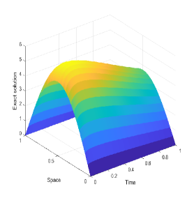
Moreover, we plot Fig. 1 to show the exact solution and numerical solutions produced by two difference schemes for Example 1. As seen from Fig. 1, the exact solution of Example 1 indeed changes dramatically near the initial time (i.e., a weak singularity near $\tau=0$ ), and numerical solutions produced by two proposed schemes can capture such a phenomena/feature well. In summary, our proposed schemes can be viewed as two robust and reliable tools for Example 1, especially the FS will be preferable because it can save much computational cost.

Table 1: Spatial convergence order of two proposed compact difference methods for Example 1 with

M(N)=\lceil N^{4/\min\{\gamma\alpha,2-\alpha\}}\rceil

and

\lambda=1

		DS (2.14)			FS (3.12)
$(\alpha,\gamma)$	$N$	$e_{\infty}(M,N)$	${Order}_{h}$	Time	$e_{\infty}(M,N)$	${Order}_{h}$	Time
(0.3, 4)	4	4.0427e-3	–	0.006	4.0427e-3	–	0.029
	8	2.5550e-4	3.9839	0.418	2.5550e-4	3.9839	0.362
	16	1.5994e-5	3.9977	33.752	1.5994e-5	3.9977	4.543
	32	9.9971e-7	3.9999	3358.44	9.9971e-7	3.9999	56.177
(0.5, 3)	6	1.8649e-3	–	0.007	1.8649e-3	–	0.028
	12	1.2337e-4	3.9180	0.199	1.2337e-4	3.9180	0.207
	24	7.9150e-6	3.9623	7.105	7.9150e-6	3.9623	1.581
	48	5.0149e-7	3.9803	291.118	5.0149e-7	3.9803	12.115
(0.8, 2)	4	3.0372e-3	–	0.006	3.0372e-3	–	0.021
	8	2.0027e-4	3.9206	0.417	2.0027e-4	3.9206	0.214
	16	1.2626e-5	3.9875	33.627	1.2626e-5	3.9875	2.572
	32	7.9200e-7	3.9948	3352.67	7.9200e-7	3.9948	31.116

Table 2: Temporal convergence order of two proposed compact difference methods for Example 1 with

N(M)=\lceil M^{\min\{\gamma\alpha,2-\alpha\}/4}\rceil

and

\lambda=1

		DS (2.14)			FS (3.12)
$(\alpha,\gamma)$	$M$	$e_{2}(M,N)$	${Order}_{\Delta\tau}$	Time	$e_{\infty}(M,N)$	${Order}_{\Delta\tau}$	$\mathrm{Time}$
(0.3, 4)	800	3.4397e-4	–	0.265	3.4397e-4	–	0.275
	1600	1.4977e-4	1.1995	0.950	1.4977e-4	1.1995	0.587
	3200	6.5200e-5	1.1998	3.485	6.5200e-5	1.1998	1.251
	6400	2.8382e-5	1.1999	13.250	2.8382e-5	1.9999	2.680
(0.5, 3)	640	1.5773e-4	–	0.138	1.5773e-4	–	0.173
	1280	5.6136e-5	1.4905	0.542	5.6136e-5	1.4905	0.363
	2560	2.0073e-5	1.4837	2.076	2.0073e-5	1.4837	0.794
	5120	7.1614e-6	1.4869	8.112	7.1614e-6	1.4869	1.693
(0.8, 2)	640	3.4921e-4	–	0.173	3.4921e-4	–	0.127
	1280	1.5606e-4	1.1620	0.626	1.5606e-4	1.1620	0.278
	2560	6.8165e-5	1.1950	2.277	6.8165e-5	1.1950	0.564
	5120	2.9334e-5	1.2164	8.578	2.9334e-5	1.2164	1.198

Refer to caption — Fig. 1: Exact and numerical solutions of Example 1 at $\alpha=0.5$ with $(\alpha,\lambda)=(0.5,1)$ , $N=24$ and $M(N)=\lceil N^{4/\min\{\gamma\alpha,2-\alpha\}}\rceil$ . Left: exact solution; Middle: DS (2.14); Right: FS (3.12).

Example 2. The second example reads the following tempered TFBS model with nonhomogeneous BCs.

\begin{cases}{}^{C}_{0}\mathbb{D}^{\alpha,\lambda}_{\tau}U(x,\tau)=\frac{\sigma^{2}}{2}\frac{\partial^{2}U(x,\tau)}{\partial x^{2}}+c\frac{\partial U(x,\tau)}{\partial x}-rU(x,\tau)+f(x,\tau),&(x,\tau)\in(0,1)\times(0,1],\\ U(x,0)=x^{4}+x^{3}+x^{2}+1,&x\in[0,1],\\ U(0,\tau)=e^{-\lambda\tau}(\tau^{\alpha}+1),\quad U(1,\tau)=4e^{-\lambda\tau}(\tau^{\alpha}+1),&\tau\in(0,1],\end{cases}

(4.2)

where the source term is defined as

\begin{split}f(x,\tau)&=e^{-\lambda\tau}\Big{[}\Gamma(1+\alpha)(x^{4}+x^{3}+x^{2}+1)-\frac{\sigma^{2}}{2}(12x^{2}+6x+2)(\tau^{\alpha}+1)-c(4x^{3}\\ &\quad~{}+3x^{2}+2x)(\tau^{\alpha}+1)+r(x^{4}+x^{3}+x^{2}+1)(\tau^{\alpha}+1)\Big{]}\end{split}

such that the exact solution of model (4.2) reads $U(x,\tau)=e^{-\lambda\tau}(\tau^{\alpha}+1)(x^{4}+x^{3}+x^{2}+1)$ . Moreover, the parameter values are $r=0.03,D=0.01$ and $\sigma=0.45$ .

To solve Example 2, we rewrite it into the equivalent form of (2.2) in order to apply the proposed schemes (2.14) and (3.12). By choosing the appropriate graded time steps, numerical results of Example 2 are listed in Tables 3–4, which demonstrate that the proposed methods work very well with the temporal $\min\{\gamma\alpha,2-\alpha\}$ -order and spatial fourth-order convergence accuracies for the tempered time-fractional TFBS model with nonhomogeneous BCs. Compared to the direct difference scheme, the fast difference scheme based on the SOE approximation of the graded L1 formula does not lose the accuracy with fitted tolerance $\epsilon$ and it also can save much computational cost in terms of the elapsed CPU time, especially when the number of time steps is increasingly large.

Table 3: Spatial convergence order of two proposed compact difference schemes for Example 2 with

M(N)=\lceil N^{4/\min\{\gamma\alpha,2-\alpha\}}\rceil

and

\lambda=1

		DS (2.14)			FS (3.12)
$(\alpha,\gamma)$	$N$	$e_{\infty}(M,N)$	${Order}_{h}$	$\mathrm{Time}$	$e_{\infty}(M,N)$	${Order}_{h}$	$\mathrm{Time}$
(0.3, 4)	4	8.5897e-4	–	0.007	8.5897e-4	–	0.028
	8	5.5574e-5	3.9501	0.414	5.5574e-5	3.9501	0.358
	16	3.4962e-6	3.9920	33.678	3.4962e-6	3.9920	4.516
	32	2.1896e-7	3.9970	3352.30	2.1896e-7	3.9970	55.893
(0.5, 3)	6	3.9132e-4	–	0.006	3.9132e-4	–	0.027
	12	2.6851e-5	3.8653	0.197	2.6851e-5	3.8653	0.201
	24	1.7280e-6	3.9578	7.134	1.7280e-6	3.9578	1.557
	48	1.0966e-7	3.9780	285.720	1.0966e-7	3.9780	11.961
(0.8, 2)	4	6.5572e-4	–	0.007	6.5572e-4	–	0.019
	8	4.3348e-5	3.9190	0.418	4.3348e-5	3.9190	0.209
	16	2.7691e-6	3.9685	33.538	2.7691e-6	3.9685	2.552
	32	1.7325e-7	3.9985	3362.85	1.7325e-7	3.9985	30.974

Table 4: Temporal convergence order of two proposed compact difference schemes for Example 2 with

N(M)=\lceil M^{\min\{\gamma\alpha,2-\alpha\}/4}\rceil

and

\lambda=1

		DS (2.14)			FS (3.12)
$(\alpha,\gamma)$	$M$	$e_{\infty}(M,N)$	$Order_{\Delta\tau}$	$\mathrm{Time}$	$e_{\infty}(M,N)$	${Order}_{\Delta\tau}$	$\mathrm{Time}$
(0.3, 4)	800	7.4809e-5	–	0.262	7.4809e-5	–	0.274
	1600	3.2779e-5	1.1904	0.943	3.2779e-5	1.1904	0.593
	3200	1.4284e-5	1.1984	3.441	1.4284e-5	1.1984	1.260
	6400	6.2129e-6	1.2011	13.112	6.2129e-6	1.2011	2.694
(0.5, 3)	640	3.4280e-5	–	0.138	3.4280e-5	–	0.169
	1280	1.2276e-5	1.4815	0.554	1.2276e-5	1.4815	0.365
	2560	4.3921e-6	1.4829	2.065	4.3921e-6	1.4829	0.782
	5120	1.5645e-6	1.4892	8.058	1.5645e-6	1.4892	1.659
(0.8, 2)	640	7.7152e-5	–	0.170	7.7152e-5	–	0.126
	1280	3.3781e-5	1.1915	0.623	3.3781e-5	1.1915	0.267
	2560	1.4712e-5	1.1992	2.263	1.4712e-5	1.1992	0.569
	5120	6.3887e-6	1.2034	8.499	6.3887e-6	1.2034	1.194

Example 3. We then consider the tempered TFBS model describing a double barrier knock-out option under a truncated domain $\widehat{\Omega}\cup\partial\widehat{\Omega}=[S_{l},S_{r}]$ , which is modified from [2].

\begin{cases}\frac{\partial^{\alpha,\lambda}C(S,t)}{\partial t^{\alpha,\lambda}}+\frac{1}{2}\sigma^{2}S^{2}\frac{\partial^{2}C(S,t)}{\partial S^{2}}+\hat{r}S\frac{\partial C(S,t)}{\partial S}-rC(S,t)=0,&(S,t)\in\widehat{\Omega}\times[0,T),\\ C(S,T)=\max(S-K,0),&S\in\widehat{\Omega},\\ C(S,t)=0,&(S,t)\in\partial\widehat{\Omega}\times[0,T),\end{cases}

(4.3)

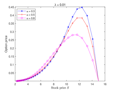
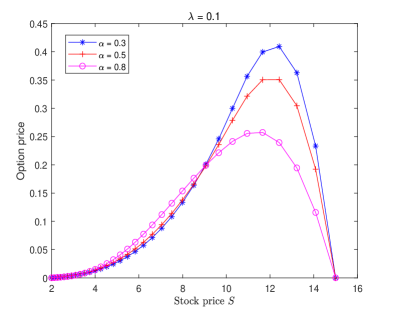
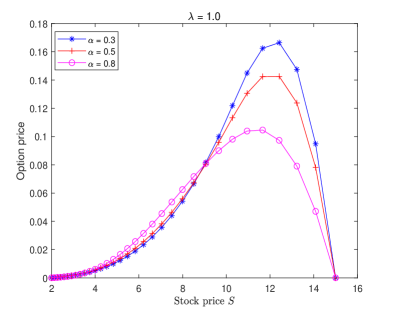
Here, the model parameters are set as $r=0.03$ , $K=10$ , $\sigma=0.45$ , $T=1$ (year), $D=0.01$ , and $(S_{l},S_{r})=(2,15)$ .

Fig. 2 displays the double barrier option price of Example 3 solved by the proposed numerical scheme (3.12) for different choices $(\alpha,\lambda)$ and fixed $N=32$ , where the grading parameter $\gamma$ and $M(N)$ time steps are chosen as Examples 1–2. It is observed that the characteristics of Figure 2 are consistent with [11, Fig. 3]. Moreover, we can find from Figure 2 that the double barrier option price will be influenced by the fractional order $\alpha$ and tempered index $\lambda$ . Compared with the classical BS and TFBS models [33, Figure 2], the tempered TFBS model does not overprice the double barrier knock-out option when the underlying is close to the lower barrier. From a certain underlying value and onwards (close to the strike price $S$ ), the tempered TFBS model also does not underprice the price of options. It can be noticed that the smaller $\alpha$ and $\lambda$ are, the larger pricing bias becomes. This suggests that the tempered TFBS model may capture the (memory) characteristics of the significant movements more accurately.

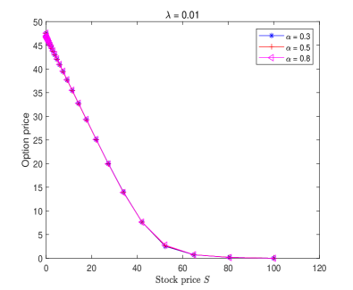
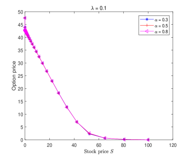
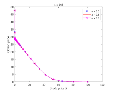
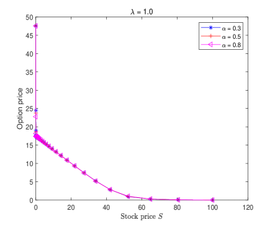
Example 4. Consider the following tempered TFBS model governing the European put options

\begin{cases}\frac{\partial^{\alpha,\lambda}C(S,t)}{\partial t^{\alpha,\lambda}}+\frac{1}{2}\sigma^{2}S^{2}\frac{\partial^{2}C(S,t)}{\partial S^{2}}+\hat{r}S\frac{\partial C(S,t)}{\partial S}-rC(S,t)=0,&(S,t)\in(0,+\infty)\times[0,T),\\ C(S,T)=\max(K-S,0),&S\in(0,+\infty),\\ C(0,t)=\phi(t),\quad\lim\limits_{S\rightarrow+\infty}C(S,t)=0,&t\in[0,T),\end{cases}

(4.4)

where the parameters are set as $r=0.05$ , $K=50$ , $\sigma=0.25$ , $D=0$ , $T=1~{}{\rm(year)}$ and $\phi(t)=Ke^{-r(T-t)}$ . In this example, we need to compute the Mittage-Lefflier (M-L) function $E_{1,2-\alpha}(z)$ ( $z\in\mathbb{R}$ ) (numerically)³³3Evaluation of the M-L function with 2 parameters: https://www.mathworks.com/matlabcentral/fileexchange/48154-the-mittag-leffler-function. when we transform this model to the equation like Eq. (2.2).

We now apply the proposed fast numerical scheme (3.12) which is better than the scheme (2.14) to solve Example 3 for different values of $(\alpha,\lambda)$ and fixed $N=32$ . The curves of the put option price are plotted in Fig. 3, where the grading parameter $\gamma$ and $M(N)$ time steps are chosen as the same as Examples 1–2. As can be seen from them, the order of fractional derivative $\alpha$ and the (large) tempered index $\lambda$ have an effect on the prices of European put options where the underlying assets display characteristic periods in which they remain motionless [36].

5 Conclusions

In this study, we proposed the direct and fast compact difference schemes with unequal time-steps for the tempered TFBS model. The numerical methods are constructed by the compact difference operator and the (fast) tempered L1 formula with nonuniform time steps for spatial and temporal derivatives, respectively. The unconditional stability and convergence of $\min\left\{\gamma\alpha,2-\alpha\right\}$ -order in time and fourth-order in space are rigorously proved by mathematical induction. Numerical examples are included and the corresponding results indicated that the proposed numerical method works very precise and fast.

In addition, since the financial payoff function of the option at the strike price is often non-smooth, the compact difference method maybe cannot reach the convergence of the fourth-order accuracy in space. Such a numerical deficiency can be remedied by using the piecewise uniform mesh [30] and/or local mesh refinement [52] and it should not affect the effectiveness of our (fast) temporal discretization. This will be our future research direction.

Appendix A Appendix

For clarity, the regularity of the solution $v$ of Eq. (2.2) is discussed in this appendix. It helps us to find that $v$ is smooth away from $\tau=0$ but it has in general a certain singular behaviour at $\tau=0$ .

Motivated by [26, 51], we use the separation of variables to construct a classical solution $v(x,\tau)$ of (2.2) in the form of an infinite series. Let $\{(\mu_{i},\psi_{i}):i=1,2,\ldots\}$ be the eigenvalues and eigenfunctions for the Sturm-Liouville two-point boundary value problem

\mathcal{L}\psi_{i}:=-\frac{\sigma^{2}}{2}\psi^{\prime\prime}_{i}+q\psi_{i}=\mu_{i}\psi_{i}~{}~{}{\rm on}~{}(x_{l},x_{r}),\quad\psi_{i}(x_{l})=\psi_{i}(x_{r})\equiv 0,

(A.1)

where the eigenfunctions are normalised by requiring $\|\psi_{i}\|_{2}=1$ for all $i$ . It is well known that $\mu_{i}>0$ for all $i$ . A standard separation of variables technique construct an infinite series solution to Eq. (2.2) with the form

v(x,\tau)=\sum^{\infty}_{i=1}v_{i}(\tau)\psi_{i}(x).

For clarity, we denote $v_{i}(\tau)=\langle v(\cdot,\tau),\psi_{i}(x)\rangle$ , $\widetilde{\sigma}_{i}=\langle\sigma(\cdot),\psi_{i}(\cdot)\rangle$ , $g_{i}(\tau)=\langle v(\cdot,\tau),\psi_{i}(\cdot)\rangle$ , $Q=\Omega\times(0,T]$ , $\bar{Q}=\bar{\Omega}\times(0,T]$ and $\bar{\Omega}=\partial\Omega\cup\Omega$ . Then we have

{}^{C}_{0}\mathbb{D}^{\alpha,\lambda}_{\tau}v_{i}(\tau)=-\mu_{i}v_{i}(\tau)+g_{i}(\tau).

With the help of Laplace transform, one obtains

(s+\lambda)^{\alpha}\hat{v}_{i}(s)-(s+\lambda)^{\alpha-1}\widetilde{\sigma}_{i}=-\mu_{i}\hat{v}_{i}(s)+\hat{g}_{i}(s),

or equivalently [53, (62)]

\hat{v}_{i}(s)=\frac{(s+\lambda)^{\alpha-1}\widetilde{\sigma}_{i}+\hat{g}_{i}(s)}{(s+\lambda)^{\alpha}+\mu_{i}}.

(A.2)

Hence, using the inverse Laplace transform and two-parameter M-L function [54] defined by

E_{\alpha,\beta}(z):=\sum^{\infty}_{k=0}\frac{z^{k}}{\Gamma(\alpha z+\beta)},\quad\Re e(\alpha)>0,~{}\Re e(\beta)>0,~{}z\in\mathbb{C},

we can obtain the following form

v(x,\tau)=\sum^{\infty}_{i=1}\left[\widetilde{\sigma}_{i}G_{i}(\tau)+F_{i}(\tau)\right]\psi_{i}(x)

(A.3)

–see [51, (2.8)]–where $G_{i}(\tau)=e^{-\lambda\tau}E_{\alpha,1}(-\mu_{i}\tau^{\alpha})$ and $F_{i}(\tau)=\int^{\tau}_{0}e^{-\lambda s}s^{\alpha-1}E_{\alpha,\alpha}(-\mu_{i}s^{\alpha})g_{i}(\tau-s)ds$ .

With the help of sectorial operator [27], for each $\nu\in\mathbb{R}$ the fractional power $\mathcal{L}^{\nu}$ of the operator $\mathcal{L}$ is defined with the domain

H(\mathcal{L}^{\nu}):=\Big{\{}g\in L_{2}(\Omega):\sum^{\infty}_{i=1}\mu^{2\nu}_{i}|\langle g,\psi_{i}\rangle|^{2}\Big{\}},

and the norm

\|g\|_{\mathcal{L}^{\nu}}=\Bigg{(}\sum^{\infty}_{i=1}\mu^{2\nu}_{i}|\langle g,\psi_{i}\rangle|^{2}\Bigg{)}^{1/2}.

Theorem A.1.

Let $v$ be the solution of Eq. (2.2). Then for $\forall\epsilon>0$ , there exists the constant $C$ independent of $\tau$ such that the following conclusions are available:

i)

if $\sigma\in H\left(\mathcal{L}^{\frac{1+\epsilon}{2}}\right),g(\cdot,\tau)\in H\left(\mathcal{L}^{\frac{1+\epsilon}{2}}\right)$ for $\forall\tau\in[0,T]$ , then $|v(x,\tau)|\leq C$ for $(x,\tau)\in\bar{Q}$ ;
ii)

if $\sigma\in H\left(\mathcal{L}^{\frac{3+\epsilon}{2}}\right),g(\cdot,\tau)\in H\left(\mathcal{L}^{\frac{1+\epsilon}{2}}\right)$ for $\forall\tau\in[0,T]$ , then $\|g_{tau}(\cdot,\tau)\|_{\mathcal{L}^{\frac{1+\epsilon}{2}}}\leq C\tau^{-\rho}$ ( $\rho<1)$ for $\forall\tau\in(0,T]$ , then $|v_{\tau}(x,\tau)\leq\tau^{\alpha-1}$ for $\forall(x,\tau)\in Q$ .

Proof: i) With the help of Eq. (A.3), the triangle inequality yields that

\begin{split}|v(x,\tau)|&=\sum^{\infty}_{i=1}|\widetilde{\sigma}_{i}G_{i}(\tau)+F_{i}(\tau)|\cdot|\psi_{i}(x)|\\ &\leq\sum^{\infty}_{i=1}\Big{[}|\widetilde{\sigma}_{i}e^{-\lambda\tau}E_{\alpha,1}(-\mu_{i}\tau^{\alpha})|~{}+\\ &\quad~{}\left|\int^{\tau}_{0}e^{-\lambda s}s^{\alpha-1}E_{\alpha,\alpha}(-\mu_{i}s^{\alpha})g_{i}(\tau-s)ds\right|\Big{]}\cdot|\psi_{i}(x)|,\end{split}

(A.4)

since $\sigma\in H(\mathcal{L}^{\frac{1+\epsilon}{2}})$ , $g(\cdot,\tau)\in H(\mathcal{L}^{\frac{1+\epsilon}{2}})$ , we have $\|\sigma\|_{L^{\frac{1+\epsilon}{2}}}\leq C$ and $\|g(\cdot,\tau)\|_{\mathcal{L}^{\frac{1+\epsilon}{2}}}\leq C$ . In conclusion, we have $\mu_{i}\approx i$ and $|\psi_{i}(x)|\leq C$ .

Consider the term in (A.4). Using the Cauchy-Schwarz inequality and [51, Lemma 2.4], we have

\begin{split}\sum^{\infty}_{i=1}|\widetilde{\sigma}_{i}e^{-\lambda\tau}E_{\alpha,1}(-\mu_{i}\tau^{\alpha})|&\leq C\sum^{\infty}_{i=1}|\widetilde{\sigma}_{i}|\cdot|E_{\alpha,1}(-\mu_{i}\tau^{\alpha})|\\ &\leq C\Bigg{(}\sum^{\infty}_{i=1}\frac{1}{\mu^{1+\epsilon}_{i}}\Bigg{)}^{1/2}\Bigg{(}\sum^{\infty}_{i=1}\mu^{1+\epsilon}_{i}|\widetilde{\sigma}_{i}|^{2}\Bigg{)}^{1/2}\\ &\leq C\|\sigma\|_{\mathcal{L}^{\frac{1+\epsilon}{2}}}.\end{split}

Similarly, we can obtain

	$\displaystyle\sum^{\infty}_{i=1}\left\|\int^{\tau}_{0}e^{-\lambda s}s^{\alpha-1}E_{\alpha,\alpha}(-\mu_{i}s^{\alpha})g_{i}(\tau-s)ds\right\|$	$\displaystyle\leq C\int^{\tau}_{0}\left\|s^{\alpha-1}\sum^{\infty}_{i=1}E_{\alpha,\alpha}(-\mu_{i}s^{\alpha})g_{i}(\tau-s)\right\|ds$
		$\displaystyle\leq C\int^{\tau}_{0}s^{\alpha-1}\Bigg{(}\sum^{\infty}_{i=1}\frac{1}{\mu^{1+\epsilon}_{i}}(E_{\alpha,\alpha}(-\mu_{i}s^{\alpha}))^{2}\Bigg{)}^{1/2}$
		$\displaystyle\quad~{}\cdot\Bigg{(}\sum^{\infty}_{i=1}\mu^{1+\epsilon}_{i}g^{2}_{i}(\tau-s)\Bigg{)}^{1/2}ds$
		$\displaystyle\leq C.$

Hence the series (A.4) is absolutely and uniformly convergence on $\bar{Q}$ , and

|v(x,\tau)|\leq C,~{}{\rm for~{}}\forall(x,\tau)\in\bar{Q}.

(A.5)

ii) Differentiating Eq. (A.3) term by term with respect to $\tau$ for $(x,\tau)\in Q$ yields

\begin{split}v_{\tau}(x,\tau)&=\sum^{\infty}_{i=1}\Big{[}-\widetilde{\sigma}_{i}e^{-\lambda\tau}\mu_{i}\tau^{\alpha-1}E_{\alpha,\alpha}(-\mu_{i}\tau^{\alpha})+e^{-\lambda\tau}\tau^{\alpha-1}E_{\alpha,\alpha}(-\mu_{i}\tau^{\alpha})g_{i}(0)~{}+\\ &\quad~{}\int^{\tau}_{0}e^{-\lambda s}s^{\alpha-1}E_{\alpha,\alpha}(-\mu_{i}s^{\alpha})g^{\prime}_{i}(\tau-s)ds\Big{]}\psi_{i}(x),\end{split}

(A.6)

where we use the fact $\frac{dE_{\alpha,1}(-\lambda\tau^{\alpha})}{d\tau}=-\lambda\tau^{\alpha-1}E_{\alpha,\alpha}(-\lambda\tau^{\alpha})$ to differentiate $E_{\alpha,1}(\cdot)$ . Based on the proof of i), it is not hard to check that

|v_{\tau}(x,\tau)|\leq C\tau^{\alpha-1},~{}{\rm for~{}}(x,\tau)\in Q.

(A.7)

Moreover, one can show that ${}^{C}_{0}\mathbb{D}^{\alpha,\lambda}_{\tau}v$ exists and $v$ is the solution of Eq. (2.2), the maximum principle guarantees the uniqueness of solution, which completes the proof. $\Box$

At this stage, we can estimate other derivatives $\frac{\partial^{2}v}{\partial\tau^{2}}$ and $\frac{\partial^{p}v}{\partial x^{p}}$ ( $p=1,2,3,4$ ) on the domain $Q$ . At present, we summarize all the above activity in the following conclusion.

Theorem A.2.

Assume that $\sigma,g(\cdot,\tau)\in H(\mathcal{L}^{\frac{5+\epsilon}{2}})$ , $g_{\tau}(\cdot,\tau)$ and $g_{\tau\tau}(\cdot,\tau)$ are in $H(\mathcal{L}^{\frac{5+\epsilon}{2}})$ for each $\tau\in(0,T]$ with

\|g(\cdot,\tau)\|_{\mathcal{L}^{\frac{5+\epsilon}{2}}}+\|g_{\tau}(\cdot,\tau)\|_{\mathcal{L}^{\frac{1+\epsilon}{2}}}+\tau^{\rho}\|g_{\tau\tau}(\cdot,\tau)\|_{\mathcal{L}^{\frac{1+\epsilon}{2}}}\leq C_{1}

for $\forall\tau\in(0,T],\forall\epsilon>0$ and the constant $\rho<1$ , where $C_{1}$ is a constant independent of $\tau$ . Then there exists a constant $C$ such that

\begin{cases}\left|\frac{\partial^{p}v(x,\tau)}{\partial x^{p}}\right|\leq C,&{\rm for}~{}p=0,1,2,3,4,\\ \left|\frac{\partial^{\ell}v(x,\tau)}{\partial\tau^{\ell}}\right|\leq C(1+\tau^{\alpha-\ell}),&{\rm for}~{}\ell=0,1,2\end{cases}

(A.8)

for $\forall(x,\tau)\in\bar{\Omega}\times(0,T]$ .

In short, we shall assume that the solution $v$ of (2.2) satisfies the bounds (A.8). Thus in general, the solution $v$ of (2.2) will have a weak singularity along $\tau=0$ . Its presence leads to significant practical and theoretical difficulties in designing and analysing numerical methods for (2.2). That is just why we consider the non-uniform temporal discretization in this paper.

Acknowledgment

The authors would like to thank anonymous reviewers, Dr. Can Li and Dr. Jinye Shen whose insightful comments and careful proof-checks helped to improve the current paper. This work was supported by the Applied Basic Research Program of Sichuan Province (2020YJ0007) and the Sichuan Science and Technology Program (2022ZYD0006). X.-M. Gu also thanks Prof. Dongling Wang for helpful discussions during his visiting to Xiangtan University.

References

[1] B. Øksendal, Stochastic Differential Equations: An Introduction with Applications, Springer Berlin, Heidelberg (2003).
[2] R. H. D. Staelen, A. S. Hendy, Numerically pricing double barrier options in a time-fractional Black-Scholes model, Comput. Math. Appl., 74(6) (2017): 1166-1175.
[3] L. Meng, M. Wang, Comparison of Black-Scholes formula with fractional Black-Scholes formula in the foreign exchange option market with changing volatility, Asia Pac. Financ. Mark., 17(2) (2010): 99-111.
[4] P. Nicolas, An Elementary Introduction to Stochastic Interest Rate Modeling (2nd ed.), Advanced Series on Statistical Science and Applied Probability, Vol. 16, World Scientific Publishing, Singapore (2012).
[5] S. G. Kou, A jump-diffusion model for option pricing, Manage. Sci., 48(8) (2002): 1086-1101.
[6] W. Wyss, The fractional Black-Scholes equation, Fract. Cal. Appl. Anal., 3(1) (2000): 51-61.
[7] G. Jumarie, Stock exchange fract ional dynamics defined as fractional exponential growth driven by (usual) Gaussian white noise. Application to fractional Black Scholes equations, Insur. Math. Econ., 42(1) (2008): 271-287.
[8] Á. Cartea, Derivatives pricing with marked point processes using tick-by-tick data, Quant. Finance, 13(1) (2013): 111-123.
[9] J.-R. Liang, J. Wang, W.-J. Zhang, W.-Y. Qiu, F.-Y. Ren, The solutions to a bi-fractional Black-Scholes-Merton differential equation, Int. J. Pure Appl. Math., 58(1) (2010): 99-112.
[10] M. Magdziarz, Black-Scholes formula in subdiffusive regime, J. Stat. Phys., 136(3) (2009): 553-564.
[11] W. Chen, X. Xu, S.-P. Zhu, Analytically pricing double barrier options based on a time-fractional Black-Scholes equation, Comput. Math. Appl., 69(12) (2015): 1407-1419.
[12] A. Farhadi, M. Salehi, G. H. Erjaee, A new version of Black-Scholes equation presented by time-fractional derivative, Iran. J. Sci. Technol. Trans. A: Sci., 42(4) (2018): 2159-2166.
[13] S. E. Fadugba, Homotopy analysis method and its applications in the valuation of European call options with time-fractional Black-Scholes equation, Chaos Solit. Fractals, 141 (2022): 110351. DOI: 10.1016/j.chaos.2020.110351.
[14] G. Krzyżanowski, M. Magdziarz, Ł. Płociniczak, A weighted finite difference method for subdiffusive Black-Scholes model, Comput. Math. Appl., 80(5) (2020): 653-670.
[15] H. Zhang, F. Liu, I. Turner, Q. Yang, Numerical solution of the time fractional Black-Scholes model governing European options, Comput. Math. Appl., 71(9) (2016): 1772-1783.
[16] Z. Tian, S. Zhai, Z. Weng, Compact finite difference schemes of the time fractional Black-Scholes model, J. Appl. Anal. Comput., 10(3) (2020): 904-919.
[17] Y. M. Dimitrov, L.G. Vulkov, Three-point compact finite difference scheme on non-uniform meshes for the time-fractional Black-Scholes equation, AIP Conf. Proc., 1690(1) (2015): 040022. DOI: 10.1063/1.4936729.
[18] K. Kazmi, A second order numerical method for the time-fractional Black-Scholes European option pricing model, J. Comput. Appl. Math., 418 (2022): 114647.
[19] P. Roul, A high accuracy numerical method and its convergence for time-fractional Black-Scholes equation governing European options, Appl. Numer. Math., 151 (2020): 472-493.
[20] N. Abdi, H. Aminikhah, A. H. Refahi Sheikhani, High-order compact finite difference schemes for the time-fractional Black-Scholes model governing European options, Chaos Solit. Fractals, 162 (2022): 112423. DOI: 10.1016/j.chaos.2022.112423.
[21] M. N. Koleva, L. G. Vulkov, Numerical solution of time-fractional Black-Scholes equation, Comput. Appl. Math., 36 (2017): 1699-1715.
[22] M. Sarboland, A. Aminataei, On the numerical solution of time fractional Black-Scholes equation, Int. J. Comput. Math., 99(9) (2022): 1736-1753.
[23] X. An, F. Liu, M. Zheng, V. V. Anh, I. W. Turner, A space-time spectral method for time-fractional Black-Scholes equation, Appl. Numer. Math., 165 (2021): 152-166.
[24] T. Akram, M. Abbas, K. M. Abualnaja, A. Iqbal, A. Majeed, An efficient numerical technique based on the extended cubic B-spline functions for solving time fractional Black-Scholes model, Eng. Comput., 38 (2022): 1705-1716.
[25] M. Rezaei, A. R. Yazdanian, A. Ashrafi, S. M. Mahmoudi, Numerical pricing based on fractional Black-Scholes equation with time-dependent parameters under the CEV model: Double barrier options, Comput. Math. Appl., 90 (2021): 104-111.
[26] M. Stynes, E. O’Riordan, J. L. Gracia, Error analysis of a finite difference method on graded meshes for a time-fractional diffusion equation, SIAM J. Numer. Anal., 55(2) (2017): 1057-1079.
[27] K. Sakamoto, M. Yamamoto, Initial value/boundary value problems for fractional diffusion-wave equations and applications to some inverse problems, J. Math. Anal. Appl., 382(1) (201): 426-447.
[28] H.-L. Liao, D. Li, J. Zhang, Sharp error estimate of the nonuniform $L1$ formula for linear reaction-subdiffusion equations, SIAM J. Numer. Anal., 56(2) (2018): 1112-1133.
[29] J.-Y. Shen, Z.-Z. Sun, R. Du, Fast finite difference schemes for the time-fractional diffusion equation with a weak singularity at the initial time, East Asia J. Appl. Math., 8(4) (2018): 834-858.
[30] Z. Cen, J. Huang, A. Xu, A. Le, Numerical approximation of a time-fractional Black-Scholes equation, Comput. Math. Appl., 75(8) (2018): 2874-2887.
[31] M. N. Koleva, L. G. Vulkov, Fast positivity preserving numerical method for time-fractional regime-switching option pricing problem, in Advanced Computing in Industrial Mathematics. BGSIAM 2020 (I. Georgiev, H. Kostadinov, E. Lilkova, eds.), Studies in Computational Intelligence, Vol. 1076. Springer, Cham (2023): 88-99. DOI: 10.1007/978-3-031-20951-2_9.
[32] M. She, L. Li, R. Tang, D. Li, A novel numerical scheme for a time fractional Black-Scholes equation, J. Appl. Math. Comput., 66(1-2) (2021): 853-870.
[33] K. Song, P. Lyu, A high-order and fast scheme with variable time steps for the time-fractional Black-Scholes equation, Math. Methods Appl. Sci., 46(2) (2023): 1990-2011.
[34] S. Jiang, J. Zhang, Q. Zhang, Z. Zhang, Fast evaluation of the Caputo fractional derivative and its applications to fractional diffusion equations, Commun. Comput. Phys., 21(3) (2017): 650-678.
[35] H.-L. Liao, W. McLean, J. Zhang, A discrete Gronwall inequality with applications to numerical schemes for subdiffusion problems, SIAM J. Numer. Anal., 57(1) (2019): 218-237.
[36] G. Krzyżanowski, M. Magdziarz, A tempered subdiffusive Black-Scholes model, arXiv preprint, arXiv:2103.13679, 22 May 2022, 27 pages.
[37] M. M. Meerschaert, A. Sikorskii, Stochastic Models for Fractional Calculus. De Gruyter Studies in Mathematics, Vol. 43, Walter de Gruyter, Berlin/Boston (2012).
[38] Á. Cartea, D. del-Castillo-Negrete, Fluid limit of the continuous-time random walk with general Lèvy jump distribution functions, Phys. Rev. E., 76(4) (2017): 041105.
[39] L. Zhao, C. Li, F. Zhao, Efficient diference schemes for the Caputo-tempered fractional difusion equations based on polynomial interpolation, Commun. Appl. Math. Comput., 3(1) (2021): 1-40. DOI: 10.1007/s42967-020-00067-5.
[40] M. M. Meerschaert, Y. Zhang, B. Baeumer, Tempered anomalous diffusion in heterogeneous systems, Geophys. Res. Lett., 35(17) (2008): L17403. DOI: 10.1029/2008GL034899.
[41] M. L. Morgado, L. F. Morgado, Modeling transient currents in time-of-flight experiments with tempered time-fractional diffusion equations, Progr. Fract. Differ. Appl., 6(1) (2020): 43-53. DOI: 10.18576/pfda/060105.
[42] J. L. Gracia, E. O’Riordan, M. Stynes, Convergence in positive time for a finite difference method applied to a fractional convection-diffusion problem, Comput. Methods Appl. Math., 18(1) (2018): 33-42.
[43] S. Franz, N. Kopteva, Pointwise-in-time a posteriori error control for higher-order discretizations of time-fractional parabolic equations, J. Comput. Appl. Math., 427 (2023): 115122. DOI: 10.1016/j.cam.2023.115122.
[44] X. Yang, L. Wu, S. Sun, X. Zhang, A universal difference method for time-space fractional Black-Scholes equation, Adv. Differ. Equ., 2016(1) (2016): 71. DOI: 10.1186/s13662-016-0792-8.
[45] X.-M. Gu, T.-Z. Huang, Y.-L. Zhao, P. Lyu, B. Carpentieri, A fast implicit difference scheme for solving the generalized time-space fractional diffusion equations with variable coefficients, Numer. Methods Partial Differ. Equ., 37(2) (2021): 1136-1162.
[46] L. Guo, F. Zeng, I. W. Turner, K. Burrage, G. E. Karniadakis, Efficient multistep methods for tempered fractional calculus: algorithms and simulations, SIAM J. Sci. Comput., 41(4) (2019): A2510-A2535.
[47] H.-L. Liao, P. Lyu, S. Vong, Y. Zhao, Stability of fully discrete schemes with interpolation-type fractional formulas for distributed-order subdiffusion equations, Numer. Algor., 75(4) (2017): 845-878.
[48] H. Chen, M. Stynes, A discrete comparison principle for the time-fractional diffusion equation, Comput. Math. Appl., 80 (2020): 917-922.
[49] B. Ji, H.-L. Liao, L. Zhang, Simple maximum principle preserving time-stepping methods for time-fractional Allen-Cahn equation, Adv. Comput. Math., 46(2) (2020): 37. DOI: 10.1007/s10444-020-09782-2.
[50] M. Stynes, A survey of the L1 scheme in the discretisation of time-fractional problems, Numer. Math. Theor. Meth. Appl., 15(4) (2022): 1173-1192.
[51] C. Wang, W. Deng, X. Tang, A sharp $\alpha$ -robust L1 scheme on graded meshes for two-dimensional time tempered fractional Fokker-Planck equation, arXiv preprint, arXiv:2205.15837v1, May 31, 2022, 25 pages.
[52] S. T. Lee, H.-W. Sun, Fourth order compact scheme with local mesh refinement for option pricing in jump-diffusion model, Numer. Methods Partial Differ. Equ., 28(2) (2012): 1079-1098.
[53] C. Li, W. Deng, L. Zhao, Well-posedness and numerical algorithm for the tempered fractional ordinary differential equations, Discrete Contin. Dyn. Syst. Ser. B, 24(4) (2015): 1989-2015.
[54] M. Ishteva, Properties and Applications of the Caputo Fractional Operator. Master thesis, Department of Mathematics, University of Karlsruhe, Karlsruhe (2005).

$\displaystyle a_{n}^{(n,\alpha)}\\|v^{n}\\|_{\infty}$	$\displaystyle\leqslant\sum_{k=1}^{n-1}(a_{k+1}^{(n,\alpha)}-a_{k}^{(n,\alpha)})\big{(}\\|v^{0}\\|_{\infty}+\Gamma(1-\alpha)\max_{1\leqslant m\leqslant k}\frac{\\|g^{m}\\|_{\infty}}{a_{1}^{(m,\alpha)}}\big{)}+a_{1}^{(n,\alpha)}\big{[}\\|v^{0}\\|_{\infty}$
	$\displaystyle+\Gamma(1-\alpha)\frac{\\|g^{n}\\|_{\infty}}{a_{1}^{(n,\alpha)}}\big{]}$
	$\displaystyle\leqslant\big{[}\sum_{k=1}^{n-1}(a_{k+1}^{(n,\alpha)}-a_{k}^{(n,\alpha)})+a_{1}^{(n,\alpha)}\big{]}\big{(}\\|v^{0}\\|_{\infty}+\Gamma(1-\alpha)\max_{1\leq m\leq n}\frac{\\|g^{m}\\|_{\infty}}{a_{1}^{(m,\alpha)}}\big{)}$
	$\displaystyle\leqslant a_{n}^{(n,\alpha)}[\\|v^{0}\\|_{\infty}+\Gamma(1-\alpha)\max_{1\leq m\leq n}\frac{\\|g^{m}\\|_{\infty}}{a_{1}^{(m,\alpha)}}].$	(2.18)