A Feature Selection Method for Multivariate Performance Measures
Abstract.
Feature selection with specific multivariate performance measures is the key to the success of many applications, such as image retrieval and text classification. The existing feature selection methods are usually designed for classification error. In this paper, we propose a generalized sparse regularizer. Based on the proposed regularizer, we present a unified feature selection framework for general loss functions. In particular, we study the novel feature selection paradigm by optimizing multivariate performance measures. The resultant formulation is a challenging problem for high-dimensional data. Hence, a two-layer cutting plane algorithm is proposed to solve this problem, and the convergence is presented. In addition, we adapt the proposed method to optimize multivariate measures for multiple instance learning problems. The analyses by comparing with the state-of-the-art feature selection methods show that the proposed method is superior to others. Extensive experiments on large-scale and high-dimensional real world datasets show that the proposed method outperforms -SVM and SVM-RFE when choosing a small subset of features, and achieves significantly improved performances over SVMperf in terms of -score.
1. Introduction
Machine learning methods have been widely applied to a variety of learning tasks (e.g. classification, ranking, structure prediction, etc) arising in computer vision, text mining, natural language processing and bioinformatics applications. Depending on applications, specific performance measures are required to evaluate the success of a learning algorithm. For instance, the error rate is a sound judgment for evaluating the classification performance of a learning method on datasets with balanced positive and negative examples. On the contrary, in text classification where positive examples are usually very few, one can simply assign all testing examples with the negative class (the major class), this trivial solution can easily achieve very low error rate due to the extreme imbalance of the data. However, the goal of text classification is to correctly detect positive examples. Hence, the error rate is considered as a poor criterion for the problems with highly skewed class distributions [11]. To address this issue, -score and Precision/Recall Breakeven Point (PRBEP) are employed as the evaluation criteria for text classification. Besides this, in information retrieval, search engine systems are required to return the top documents (images) with the highest precision because most users only scan the first few of them presented by the system, so precision/recall at are preferred choices.
Instead of optimizing the error rate, Support Vector Machine for multivariate performance measures () [11] was proposed to directly optimize the losses based on a variety of multivariate performance measures. A smoothing version of [37] was proposed to accelerate the convergence of the optimization problem specially designed for PRBEP and area under the Receiver Operating Characteristic curve (AUC). Structural SVMs are considered as the general framework for optimizing a variety of loss functions [27, 13, 28]. Other works optimize specific multivariate performance measures, such as F-score [21], normalize discount cumulative gain (NDCG) [29], ordinal regression [12], ranking loss [16] and so on.
For some real applications, such as image and document retrievals, a set of sparse yet discriminative features is a necessity for rapid prediction on massive databases. However, the learned weight vector of the aforementioned methods is usually non-sparse. In addition, there are many noisy or non-informative features in text documents and images. Even though the task-specific performance measures can be optimized directly, learning with these noisy or non-informative features may still hurt both prediction performance and efficiency. To alleviate these issues, one can resort to embedded feature selection methods [15], which can be categorized into the following two major directions.
One way is to consider the sparsity of a decision weight vector w by replacing -norm regularization in the structural risk functional (e.g. SVM, logistic regression) with -norm [39, 8, 23]. A thorough study to compare several recently developed -regularized algorithms has been conducted in [33]. According to this study, coordinate descent method using one-dimensional Newton direction (CDN) achieves the state-of-the-art performance by solving -regularized models on large-scale and high-dimensional datasets. To achieve a sparser solution, the Approximation of the zeRO norm Minimization (AROM) was proposed [30] to optimize models. Its resultant problem is non-convex, so it easily suffers from local optima. However, the recent results [18] and theoretical studies [17, 36] have showed that models (where ) even with a local optimal solution can achieve better prediction performance than convex models, which are asymptotically biased [18].
Another way is to sort the weights of a SVM classifier and remove the smallest weights iteratively, which is known as SVM with Recursive Feature Elimination (SVM-RFE) [9]. However, as discussed in [32], such nested “monotonic” feature selection scheme leads to suboptimal performance. Non-monotonic feature selection (NMMKL) [32] has been proposed to solve this problem, but each feature corresponding to one kernel makes NMMKL infeasible for high-dimensional problems. Recently, Tan et al. [26] proposed Feature Generating Machine (FGM), which shows great scalability to non-monotonic feature selection on large-scale and very high-dimensional datasets.
The aforementioned feature selection methods [33, 30, 9, 32, 26] are usually designed for optimizing classification error only. To fulfill the needs of different applications, it is imperative to have a feature selection method designed for optimizing task-specific performance measures.
To this end, we first propose a generalized sparse regularizer for feature selection. After that, a unified feature selection framework is presented for general loss functions based on the proposed regularizer. Particularly, in this paper, optimizing multivariate performance measures is studied in this framework. To our knowledge, this is the first work to optimize multivariate performance measures for feature selection. Due to exponential number of constraints brought by non-smooth multivariate loss functions [11, 13] and exponential number of feature subset combinations [26], the resultant optimization problem is very challenging for high-dimensional data. To tackle this challenge, we propose a two-layer cutting plane algorithm, including group feature generation (see Section 5.1) and group feature selection (see Section 5.2), to solve this problem effectively and efficiently. Specifically, Multiple Kernel Learning (MKL) trained in the primal by cutting plane algorithm is proposed to deal with exponential size of constraints induced by multivariate losses.
This paper is an extension of our preliminary work [19]. The main contributions of this paper are listed as follows.
-
•
The implementation details and the convergence proof of the proposed two-layer cutting plane algorithm and MKL algorithm trained in the primal are presented.
-
•
Connections to a variety of the state-of-the-art feature selection methods including SKM [3], NMMKL [32], -SVM [33], -SVM [30] and FGM [26] are discussed in details. By comparing with these methods, the advantages of our proposed methods are summarized as follows:
-
-
(1)
The tradeoff parameter in SVM [33] is too sensitive to be tuned properly since it controls both margin loss and the sparsity of . However, our method alleviates this problem by introducing an additional parameter to control the sparsity of . This separation makes parameter tuning for our methods much easier than those of SKM [3] and SVM.
-
(2)
NMMKL [32] uses the similar parameter separation strategy, but it is intractable for this method to handle high-dimensional datasets, let alone optimize multivariate losses. The proposed method can readily optimize multivariate losses for high-dimensional problems.
-
(3)
FGM [26] is a special case of the propose framework when optimizing square hinge loss with indicator variables in integer domain. The proposed framework is formulated in the real domain for general loss functions. In particular, we provide a natural extension of FGM for multivariate losses.
-
(4)
The proposed framework can be interpreted by -norm constraint, so it can be considered as one of methods. This gives another interpretation of the additional parameter .
-
-
•
Recall that Multiple-Instance Learning via Embedded instance Selection (MILES) [6], which transforms multiple instance learning (MIL) into a feature selection problem by embedding bags into an instance-based feature space and selecting the most important features, achieves state-of-the-art performance for multiple instance learning problems. Under our unified feature selection framework, we extend MILES and study MIL for multivariate performance measure. To our best knowledge, this is seldom studied in MIL scenarios, but it is important for the real world applications of MIL tasks.
-
•
Extensive experiments on several challenging and very high-dimensional real world datasets show that the proposed method yields better performance than the state-of-the-art feature selection methods, and outperforms SVMperf using all features in terms of multivariate performance measures. The experimental results on the multiple instance dataset show that our proposed method achieves promising results.
The rest of the paper is organized as follows: We briefly review in Section 2. We then introduce the proposed generalized sparse regularizer in Section 3. In particular, we study the feature selection framework for multivariate performance measures, its algorithm and its application to multiple instance learning in Section 4, 5 and 7, respectively. Section 6 gives the analysis of connections to a variety of feature selection methods. The extensive empirical results are shown in Section 8. Finally, conclusive remarks are presented in the last section.
In the sequel, means that the matrix is symmetric and positive semidefinite (psd). We denote the transpose of a vector/matrix by the superscript T and norm of a vector v by . Binary operator represents the elementwise product between two vectors/matrices.
2. SVM for Multivariate Performance Measure
Given a training sample of input-output pairs for drawn from some fixed but unknown probability distribution with and . The learning problem is treated as a multivariate prediction problem by defining the hypotheses that map a tuple of feature vectors to a tuple of labels where and . The linear discriminative function of SVMperf is defined as
| (1) |
where is the weight vector.
To learn the hypothesis (1) from training data, large margin method is employed to obtain the good generalization performance by enforcing the constraints that the decision value of the ground truth labels should be larger than any possible labels , i.e., , where is some type of multivariate loss functions (several instantiated losses are presented in Section 5.4). Structural SVMs [28, 13] are proposed to solve the corresponding soft-margin case by -slack variable formula as,
| (2) | |||||
| s.t. |
where is a regularization parameter that trades off the empirical risk and the model complexity.
The optimization problem (2) is convex, but there is the exponential size of constraints. Fortunately, this problem can be solved in polynomial time by adopting the sparse approximation algorithm of structural SVMs. As shown in [11], optimizing the learning model subject to one specific multivariate measure can really boost the performance of this measure.
3. Generalized Sparse Regularizer
In this paper, we focus on minimizing the regularized empirical loss functional as
| (3) |
where is a regularization function and is any loss function, including multivariate performance measure losses.
Since -norm regularization is used in (2), the learned weight vector w is non-sparse, and so the linear discriminant function in (1) would involve many features for the prediction. As discussed in Section 1, selecting a small set of discriminative features is crucial to many real applications. In order to enforce the sparsity on w, we propose a new sparse regularizer
where is in the real domain of , and are two parameters. The optimal solution of the new proposed regularizer should satisfy if since with induces , otherwise the objective value approaches to infinite. The -norm constraint and will force some to be zero, so the corresponding is zero, . Hence, the parameter is interpreted as a budget to control the sparsity of .
This regularizer is similar to SimpleMKL [24] with each feature corresponding to one kernel, but SimpleMKL is a special case of with , which also can be interpreted by the quadratic variational formulation of norm [2]. However, it is different from when . To explain the difference, we consider the problem (2) under the general framework (3). In the separable case, parameter does not affect the optimum solution since the error . If norm is applied to replace in Problem (2), the sparsity of will be fixed once optimal solution is reached. Hence, parameter in now can be considered as the only factor to enforce sparsity on . However, in the non-separable case where errors are allowed, parameter will also influence the sparsity of , but is expected to enforce the sparsity of more explicitly when becomes larger. This argument will be empirically justified in Section 8.1.
The learning algorithm with the proposed generalized sparse regularizer is formulated as
| (4) |
This formulation is more general for feature selection.
Lemma 1.
If , Problem (4) is jointly convex with respect to w and ; otherwise, it is not jointly convex.
Proof.
We only need to prove that, if , where is jointly convex with respect to and . The convexity of in its domain is established when the following holds: which is equivalent to for any nonzero vector . WLOG, we assume where is any real number, then this condition is reduced to: This condition always holds when , which completes the proof. ∎
In what follows, we focus on the convex formulation with . In Section 6, we will discuss the relationships with a variety of the state-of-the-art feature selection methods.
4. Feature Selection for Multivariate Performance Measures
To optimize the multivariate loss functions and learn a sparse feature representation simultaneously, we propose to solve the following jointly convex problem over and in the case of ,
| (5) | |||||
| s.t. |
The partial dual with respect to is obtained by Lagrangian function with dual variables and as follows: As the gradients of Lagrangian function with respect to vanish at the optimal points, we obtain the KKT conditions: By substituting KKT conditions back to , we obtain the dual problem as
| (6) |
where , if ,
, , and . Problem (6) is a challenging problem because of the exponential size of and high-dimensional vector for high-dimensional problems.
5. Two-Layer Cutting Plane Algorithm
In this section, we propose a two-layer cutting plane algorithm to solve Problem (6) efficiently and effectively. The two layers, namely group feature generation and group feature selection, will be described in Section 5.1 and 5.2, respectively. The two-layer cutting plane algorithm will be presented in Section 5.3 and 5.4.
5.1. Group Feature Generation
By denoting , Problem (6) turns out to be
Since domains and are nonempty, the function is closed and convex for all given any , and the function is closed and concave for all given any , the saddle-point property: holds [4].
We further denote , and then the equivalent optimization problems are obtained as
| (7) | or |
Cutting plane algorithm [14] could be used here to solve this problem. Since , the lower bound approximation of (30) can be obtained by . Then we minimize Problem (30) over the set by,
| (8) | or |
As from [22], such cutting plane algorithm can converge to a robust optimal solution within tens of iterations with the exact worst-case analysis. Specifically, for a fixed , the worst-case analysis can be done by solving,
| (9) |
which is referred to as the group generation procedure. Even though Problem (8) and (9) cannot be solved directly due to the exponential size of , we will show that they are readily solved in Section 5.2 and Section 5.4, respectively.
5.2. Group Feature Selection
However, due to the exponential size of , the complexity of Problem (29) remains. In this case, state-of-the-art multiple kernel learning algorithms [25, 24, 31] do not work any more. The following proposition shows that we can indirectly solve Problem (29) in the primal form.
Proposition 1.
The detailed proof of Proposition 1 is given in the supplementary material.
Here, we define the regularization term as with and the empirical risk function as
| (13) |
which is a convex but non-smooth function w.r.t . Then we can apply the bundle method [27] to solve this primal problem. Problem (A) is transformed as
Since is a convex function, its subgradient exists everywhere in its domain [10]. Suppose is a point where is finite, we can formulate the lower bound according to the definition of subgradient,
where subgradient is at . In order to obtain , we need to solve the following inference problem
| (14) |
which is a problem of integer programming. We delay the discussion of this problem to Section 5.4. After that, we can obtain the subgraident , so that .
Given the subgradient sequence , the tighter lower bound for can be reformulated as follows,
where . Following the bundle method [27], the criterion for selecting the next point is to solve the following problem,
| (15) | |||||
| s.t. |
The following Corollary shows that Problem (15) can be easily solved by QCQP solvers, and the number of variables is independent of the number of examples.
Corollary 1.
The proof of Corollary 1 follows the same derivation of Proposition 1 with , and the size of as . Consequently, the primal variables are recovered by .
Let , the -optimal condition in Algorithm 1 is . The convergence proof in [27] does not apply in this case as the Fenchel dual of fails to satisfy the strong convexity assumption if . As , Algorithm 1 is exactly the bundle method [27]. When , we can adapt the proof of Theorem in [13] for the following convergence results.
Theorem 1.
For any and any training example , Algorithm 1 converges to the desired precision after at most,
iterations. , and is the integer ceiling function.
Proof.
We adapt the proof of Theorem 5 in [13], and sketch the necessary changes corresponding to Problem (A). For a given set , the dual objective of can be reformulated as
Since there are the constrained quadratic problems, we consider each at one time as , where is positive semi-definite, and derivative . The Lemma 2 in [13] states that a line search starting at along an ascent direction with maximum step-size improves the objective by at least If we consider subgradient descent method, the line search along the subgradient of objective is where . Therefore, the maximum improvement is
| (17) | |||||
We can see that it is a special case of [13] if . According to Theorem 5 in [13], for a newly added constraint and some , we can obtain by setting the ascent direction for the newly added and for the others. Here, we set so as to be the lower bound of . In addition, the upper bound for can also be obtained by the fact that . By substituting them back to (17), the similar result shows the increase of the objective is at least
Moreover, the initial optimality gap is at most . Following the remaining derivation in [13], the overall bound results are obtained. ∎
Remark : Problem (15) is similar to Support Kernel Machine (SKM) [3] in which the multiple Gaussian kernels are built on random subsets of features, with varying widths. However, our method can automatically choose the most violated subset of features as a group instead of a subset of random features. Such random features lead to a local optimum; while our method could guarantee the -optimality stated in Theorem 1. However, due to the extra cost of computing nonlinear kernel, the current model are only implemented for linear kernel with learned subsets of features.
Remark : The original Problem (30) could be easily formulated as a QCQP problem with exponential size of variables needed to be optimized and huge number of base kernels in the quadratic term. Unfortunately, the standard MKL methods cannot handle Problem (30) even for a small dataset, let alone the standard QCQP solver. However, Corollary 1 makes it practical to solve a sequence of small QCQP problems directly using standard off-line QCQP solvers, such as Mosek. Note that state-of-the-art MKL solvers can also be used to solve the small QCQP problems, but they are not preferred because their solutions are less accurate than that of standard QCQP solvers, which can solve Problem (16) more accurately in this case.
5.3. The Proposed Algorithm
Algorithm 1 can obtain the -optimal solution for the original dual problem (8). By denoting , the group feature generation layer can directly use the -optimal solution of the objective to approximate the original objective . The two-layer cutting plane algorithm is presented in Algorithm 2.
From the description of Algorithm 2, it is clear to see that groups are dynamically generated and augmented into active set for group selection.
In terms of the convergence proof of FGM in [26] and Theorem 1, we can obtain the following theorem to illustrate the approximation with an -optimal solution to the original problem.
Theorem 2.
The detailed proof of Theorem 2 is given in the supplementary material.
5.4. Finding the Most Violated and d
Algorithm 1 and Algorithm2 need to find the most violated and d, respectively. In this subsection, we discuss how to obtain these quantities efficiently. Algorithm 1 needs to calculate the subgradient of the empirical risk function . Since is a pointwise supremum function, the subgradient should be in the convex hull of the gradient of the decomposed functions with the largest objective. Here, we just take one of these subgradients by solving
| (18) |
where . After obtaining , it is easy to compute and .
For finding the most violated , it depends on how to define the loss in Problem (18). One of the instances is the Hamming loss which can be decomposed and computed independently, i.e., , where is an indicator function with if , otherwise . However, there are some multivariate performance measures which could not be solved independently. Fortunately, there are a series of structured loss functions, such as Area Under ROC (AUC), Average Precision (AP), ranking and contingency table scores and other measures listed in [11, 34, 27], which can be implemented efficiently in our algorithms. In this paper, we only use several multivariate performance measures based on contingency table as the showcases and their finding could be solved in time complexity [11].
Given the true labels y and predicted labels , the contingency tables is defined as follows
| y=1 | y=-1 | |
|---|---|---|
| y’=1 | a | b |
| y’=-1 | c | d |
-score: The -score is a weighted harmonic average of Precision and Recall. According to the contingency table, we can obtain The most common choice is . The corresponding balanced measure loss can be written as . Then, Algorithm 2 in [11] can be directly applied.
Precision/Recall@k: In search engine systems, most users scan only the first few links that are presented. In this situation, Prec@k and Rec@k measure the precision and recall of a classifier that predicts exactly documents, i.e., and subject to . The corresponding loss could be defined as and . And the procedure of finding most violated y is similar to F-score, while the only difference is keeping constraint and removing .
Precision/Recall Break-Even Point (PRBEP): The Precision/Recall Break-Even Point requires that the precision and its recall are equal. According to above definition, we can see PRBEP only adds a constraint , or . The corresponding loss is defined as . Finding the most violated y should enforce the constraint .
After iterations in Algorithm 2, we transform in Problem (9) from the exponential size to a small size . Now, finding the most violated d becomes
where . With the budget constraint in , (5.4) can be solved by first sorting ’s in the descent order and then setting the first numbers corresponding to to and the rest to . This takes only operations.
6. Relations To Existing Methods
In this section, we will discuss the relationships between our proposed method for multivariate loss (5) and the state-of-the-art feature selection methods including SKM [3], NMMKL [32], -SVM [33], -SVM [30] and FGM [26]. It can be easily adapted to the general framework (4).
6.1. Connections to SKM and SVM
Let be in the real domain. We observe that when . According to [24], we transform Problem (5) in the special case of to the following equivalent optimization problem,
| (20) | |||||
| s.t. |
SKM [3] attempts to obtain the sparsity of by penalizing the square of a weighted block -norm where is the number of groups and is the weight vector for the features in the th group. The regularizer used in (20) is the square of the norm , which is a special case of SKM when and , i.e., each group contains only one feature. Minimizing the square of the -norm is very similar to -norm SVM [33] by setting with the non-negative (convex) loss function.
Regardless of -norm or the square of -norm, the parameter is too sensitive to be tuned properly since it controls both margin loss and the sparsity of . However, our method alleviates this problem by two parameters and which control margin loss and sparsity of , respectively. This separation makes parameter tuning of our method easier than those of SKM and SVM.
6.2. Connection to NMMKL
Instead of directly solving Problem (20), we formulate a more general problem (5) by introducing an additional budget parameter , which directly controls the sparsity of . The advantage is to make parameter tuning easily done since is not sensitive to the sparsity of . This strategy is also used in NMMKL [32], but one feature corresponding to one base kernel makes NMMKL intractable for high-dimensional problems. The multivariate loss is even hard to be optimized by NMMKL since there are exponential dual variables in the dual form of NMMKL from the exponential number of constraints. However, our method can readily optimize multivariate loss on high-dimensional data.
6.3. Connection to FGM
According to the work [40], we can reformulate Problem (20) as an equivalent optimization problem
| (21) | |||||
After the substitutions of and the general case of , we can obtain the following problem
| (22) | |||||
where . After deriving Lagrangian dual problem of (22), we observe that it is same as Problem (6). Problem (5.4) always finds the most violated in the integer domain , so the solutions of the following problem solved by the proposed two-layer cutting plane algorithm is the same as the solutions of Problem (6)
| (23) | |||||
where the integer domain . This formula can be equally derived as the extension of FGM for multivariate performance measures by defining the new hypotheses
| (24) |
where and . It is not trivial to perform the extension of FGM to optimize multivariate loss because original FGM method [26] cannot directly apply to solve the exponential number of constraints. And our domain of is in real domain which is more general than the integer domain used in FGM and the proposed extension (23), even though the final solutions of (5) and (23) are the same.
6.4. Connection to SVM
The following Lemma indicates that the proposed formula can be interpreted by -norm constraint.
Lemma 2.
(23) is equivalent to the following problem
| s.t. | ||||
Proof.
Note, at the optimality of (22), WLOG, suppose , the corresponding must be 0. Thus, . Let , we have Moreover, at the optimality. Therefore, the optimal solution of (22) is a feasible solution of (2). On the other hand, for the optimal in (2), let and where if ; otherwise, 0. So, the optimal solution of (2) is a feasible solution of (22). ∎
This gives another interpretation of parameter from the perspective of -norm. Since -norm represents the number of non-zero entries of , so in our method can be considered as the parameter which directly controls the sparsity of .
7. Multiple Instance Learning for Multivariate Performance Measures
We have already illustrated the proposed framework by optimizing multivariate performance measures for feature selection in Section 4. In this section, we extend this approach to solve multiple instance learning problems which have been employed to solve a variety of learning problems, e.g., drug activity prediction [7], image retrieval [35], natural scene classification [20] and text categorization [1], but it is seldom optimized for multivariate performance measures in the literature. However, it is crucial to optimize the task specific performance measures, e.g., score is widely considered as the most important evaluation criterion for a learning method in image retrieval.
Multi-instance learning was formally introduced in the context of drug activity prediction [7]. In this learning scenario, a bag is represented by a set of instances where each instance is represented by a feature vector. The classification label is only assigned to each bag instead of the instances in this bag. We name a bag as a positive bag if there is at least one positive instance in this bag, otherwise it is called negative bag. The learning problem is to decide whether the given unlabeled bag is positive or not. By defining a similarity measure between a bag and an instance, Multiple-Instance Learning via Embedded instance Selection (MILES) [6] successfully transforms multiple instance learning into a feature selection problem by embedding bags into an instance-based feature space and selecting the most important features.
Before discussing the transformation in MILES, we first give the notations of multiple instance learning problem. Following the notations in [6], we denote th positive bags as which consists of instances . Similarly, the th negative bags is denoted as . All instances belongs to the same feature space . The number of positive bags and negative bags are and , respectively. The instances in all bags are rearranged as where .
By considering each instance in the training bags as a candidate for target concepts, the embedded feature space is represented as
| (26) |
where the similarity measure between the bag and the instance is defined as the most-likely-cause estimator
| (27) |
It follows the intuition that the similarity between a concept and a bag is determined by the concept and the closest instance in this bag. The corresponding labels are constructed as follows: if is a positive bag, otherwise . For a given positive bags and negative bags, we form a new classification representation of the multiple instance learning problem as . For each instance , the new feature representation corresponds to the values of the th feature variable is
where the feature induced by provides the useful information for separating the positive and negative bags. The linear discriminant function
| (28) |
where and are the model parameters. The embedding induces a possible high-dimensional space when the number of instances in the training set is large. Since some instances may not be responsible for the label of the bags or might be similar to each other, many features are redundant or irrelevant, so MILES employs -SVM to select a subset of mapped features that is most relevant to the classification problem. However, -SVM cannot fulfill to obtain a high performance over the task-specific measures because it only focuses on optimizing zero-one loss function. Our proposed Algorithm 2 is a natural alternative feature selection method for multi-variate performance measures. The proposed algorithm for multiple instance learning to optimize multivariate measures is shown in Algorithm 3.
According to Algorithm 3, we do not need the model parameter since the structural SVM is irrelevant to the relative offset , i.e., .
8. Experiments
| Dataset | #classes | #features | #train | #test |
|---|---|---|---|---|
| points | points | |||
| News20.binary | 2 | 1,355,191 | 11,997 | 7,999 |
| URL1 | 2 | 3,231,961 | 20,000 | 20,000 |
| Image | 5 | 10,800 | 1,200 | 800 |
| Sector | 105 | 55,197 | 6,412 | 3,207 |
| News20 | 20 | 62,061 | 15,935 | 3,993 |
In this Section, we conduct extensive experiments to evaluate the performance of our proposed method and state-of-the-art feature selection methods: 1) SVM-RFE [9]; 2) -SVM; 3) FGM [26]; 4) -bmrm-F1111http://users.cecs.anu.edu.au/˜chteo/BMRM.html, which is regularized SVM for optimizing F1 score by bundle method [27]. SVM-RFE and FGM use Liblinear software 222http://www.csie.ntu.edu.tw/˜cjlin/liblinear/ as the QP solver for their SVM subproblems. For -SVM, we also use Liblinear software, which implements the state-of-the-art -SVM algorithm [33]. In addition to the comparison for - loss, we also perform experiments on image data for F1 measure. Furthermore, several specific measures on the contingency table are investigated on Text datasets by comparing with [11]. All the datasets shown in Table 1 are of high dimensions.
For convenience, we name our proposed two-layer cutting plane algorithm , where represents different type of multivariate performance measures. We implemented Algorithm 2 in MATLAB for all the multivariate performance measures listed above, using Mosek as the QCQP solver for Problem (16) which yields a worse-case complexity of . Removing inactive constraints from the working set [13] in the inner layer is employed for speedup the QCQP problem. Since the values of both and are much smaller than the number of examples and its dimensionality , the QCQP is very efficient as well as more accurate for large-scale and high-dimensional datasets. Furthermore, the codes simultaneously solve the primal and its dual form. So the optimal and can be obtained after solving Problem (16).
For a test pattern x, the discriminant function can be obtained by where , , and . This leads to the faster prediction since only a few of the selected features are involved. After computing , the matrices of Problem (16) can be incrementally updated, so it can be done totally in .
 |
|
|---|---|
| (a) | (b) |
 |
|
| (c) | (d) |
8.1. Parameter Sensitivity Analysis
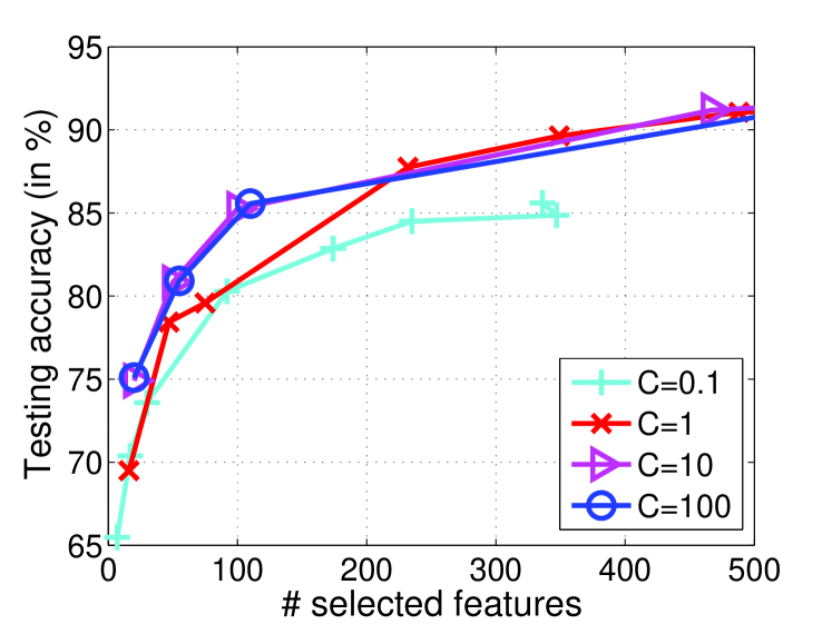
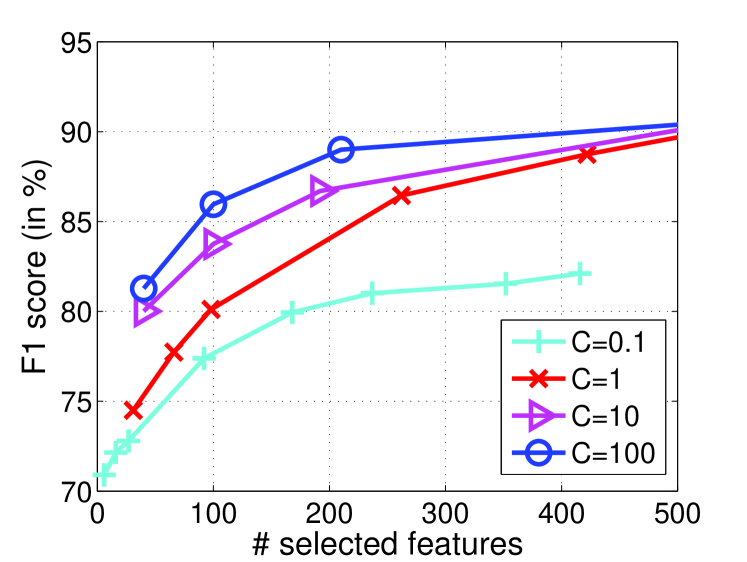
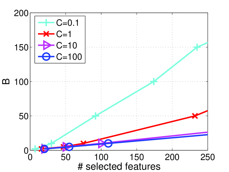
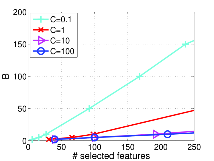
Before comparing with other methods, we first conduct empirical studies for the parameter sensitivity analysis on News20.binary. The goal is to examine the relationships among parameters and , performance measures and the number of selected features with the range of in and in .
Figure 1(a-b) show the testing accuracy and F1 scores as well as the number of selected features by varying and . We observe that the results are very sensitive to when is very small. This indicates that the model, which is equivalent to the proposed method in the case of , is vulnerable to the choice of . On the other hand, the results are rather insensitive to when is large. Hence, the proposed method is less sensitive to than model. We also observe that the proposed method prefers a large value for better performances. Figure 1(c-d) demonstrate the corresponding relationships among parameters , and the number of selected features of Figure 1(a-b). We observe that and the number of selected features always exhibits a linear trend with a constant slope. Moreover, the slope remains the same when , but a small will increase the slope. This means that, compared with , parameter has less influence on the sparsity of , and the learned feature selection model becomes stabilized when . These empirical results are consistent to the discussions of parameter in Section 3.
Since large needs more iterations to converge according to Theorem 1, the compromise is to set not too large and let dominate the selection of features. According to these observations, we can safely fix and study the results by varying to compare with other methods in the following experiments.
8.2. Time Complexity Analysis
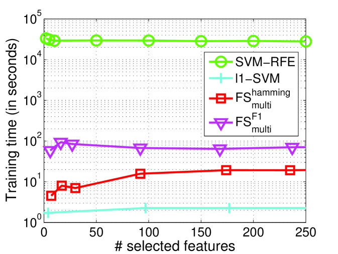 |
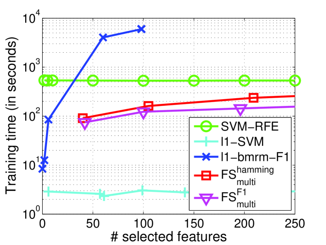
|
| (a) News20.binary | (b) Image (Desert) |
We empirically study the time complexity of by comparing with other methods. Two datasets News20.binary and Image (Desert) are used for illustration. The detailed setting are shown in Section 8.3 and Section 8.4, respectively. Figure 2 gives the training time over five different methods. On News20.binary dataset, we cannot report the training time for -bmrm-F1 since -bmrm-F1 cannot terminate after more than two days with the maximum iteration and parameter due to the extremely high dimensionality. We observe that the proposed methods are slower than -SVM, but much faster than SVM-RFE and -bmrm-F1. In addition, on Image dataset, when the termination condition with the relative difference between the objective and its convex linear lower bound lower than is set, -bmrm-F1 also cannot converge after the maximum iteration, which is consistent with the discussion in Appendix C of [27] that bundle method with regularizer cannot guarantee the convergence. This leads to the similar number of selected features (e.g., in Figure 2(b)) even though is decreasing gradually.
These observations implies that our proposed two-layer cutting plane method needs less time for training with guaranteed convergence than bundle method. Moreover, our method can work on large scale and high dimensional data for optimizing user-specified measure, but bundle method cannot. As aforementioned, -bmrm-F1 is much slower on the high dimensional datasets in our experiments, so we can only report its results in Section 8.4.
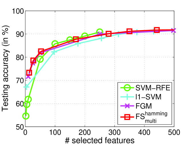
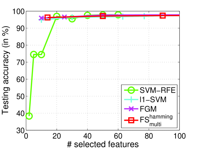
8.3. Feature Selection for Accuracy
Since [11] has proven that with Hamming loss, namely , is the same as SVM. In this subsection, we evaluate the accuracy performances of for Hamming loss function, namely as well as other state-of-the-art feature selection methods. We compare these methods on two binary datasets, News20.binary 333http://www.csie.ntu.edu.tw/˜cjlin/libsvmtools/datasets and URL1 in Table 1. Both datasets are used in [26], and they are already split into training and testing sets.
We test FGM and SVM-RFE in the grid and choose which gives good performance for both FGM and SVM-RFE. This is the same as [26]. For , we do the experiments by fixing as for URL1 and for New20.binary. The setting for budget parameter for News20.binary, and for URL1. The elimination scheme of features for SVM-RFE method can be referred to [26]. For -SVM, we report the results of different values so as to obtain different number of selected features.
 |
|
| (a) News20.binary | (b) URL1 |
|
|
| (a) News20.binary | (b) URL1 |
Figure 3 reports testing accuracy on different datasets. The testing accuracy is comparable among different methods, but both and FGM can obtain better prediction performances than SVM-RFE in a small number (less than 20) of selected features on both News20.binary and URL1. These results show that the proposed method with Hamming loss can work well on feature selection tasks especially when choosing only a few features. also performs better than -SVM on News20.binary in most range of selected features. This is possibly because models are more sensitive to noisy or redundant features on News20.binary dataset.
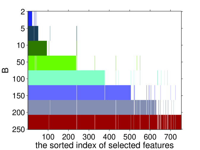
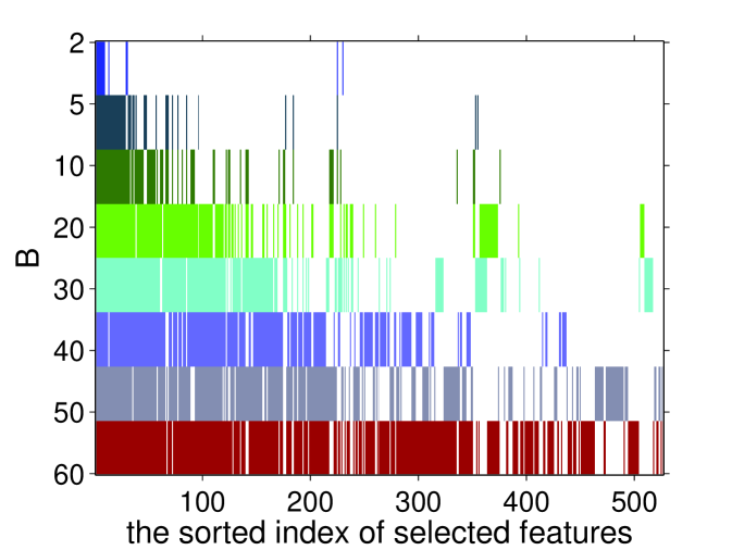
Figure 4 shows that our method with the small will select smaller number of features than the large . We also observed that most of features selected by the small also appeared in the subset of features using the large . This phenomenon can be obviously observed on News20.binary. This leads to the conclusion that can select the important features in the given datasets due to the insensitivity of parameter . However, we notice that not all the features in the selected subset of features with smaller fall into that of subset of features with the large , so our method is non-monotonic feature selection. This argument is consistent with the test accuracy in Figure 3. News20.binary seems to be monotonic datasets from Figure 4, since , FGM and SVM-RFE demonstrate similar performance. However, URL1 is more likely to be non-monotonic, as our method and FGM can do better than SVM-RFE. All the facts imply that the proposed method is comparable with FGM and SVM-RFE. And it also demonstrates the non-monotonic property for feature selection.
8.4. Feature Selection for Image Retrieval
 |
|
| (a) Desert | (b) Mountains |
 |
|
| (c) Sea | (d) Sunset |
 |
|
| (e) Trees | |
| Dataset | method | #selected features | |||
|---|---|---|---|---|---|
| 92.07 | 95.77 | 93.25 | 787.6/658.9/508.3 | ||
| Sector | 84.99 | 90.01 | 85.54 | 689.2 | |
| 33.35 | 95.52 | 91.24 | 55,197 | ||
| 77.56 | 91.21 | 81.46 | 1,301 / 1,186 / 931 | ||
| News20 | 49.61 | 66.32 | 52.14 | 485.1 | |
| 55.53 | 93.08 (16/2) | 80.83 (6/11) | 62,061 |
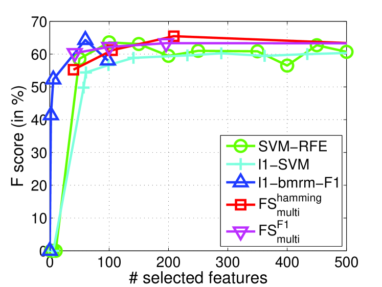
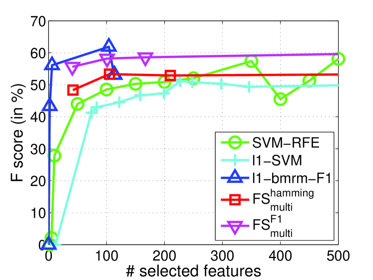
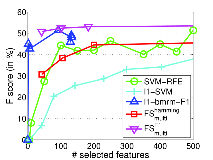
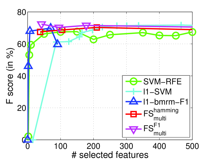
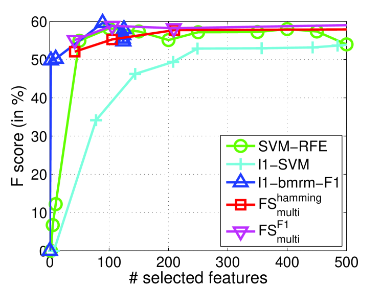
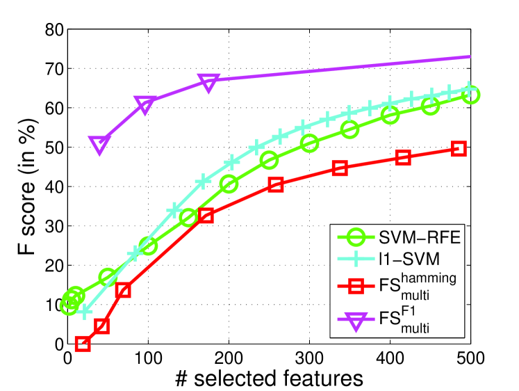
In this subsection, we demonstrate the specific multivariate performance measures are important to select features for real applications. In particular, we evaluate measure (commonly used performance measure) for the task of image retrieval. Due to the success of transforming multiple instance learning into a feature selection problem by embedded instance selection, we use the same strategy in Algorithm 4.1 of [6] to construct a dense and high-dimensional dataset on a preprocessed image data 444http://lamda.nju.edu.cn/data_MIMLimage.ashx. This dataset is used in [38] for multi-instance learning. It contains five categories and images. Each image is represented as a bag of nine instances generated by the SBN method [20]. Each image bag is represented by a collection of nine 15-dimensional feature vectors. After that, following [6], the natural scene image retrieval problem turns out to be a feature selection task to select relevant embedded instances for prediction. The Image dataset are split randomly with the proportion of 60% for training and 40% for testing (Table 1). Since -score is used for performance metric, we perform for -score, namely as well as other state-of-the-art feature selection methods. As mentioned above, FGM and have similar performances, we will not report the results of FGM here. and use the fixed . For other methods, we use the previous settings. The testing values of all methods on each category are reported in Figure 5.
From Figure 5, we observe that and achieve significantly improved performance over -SVM in term of -score especially when choosing less than features. Moreover, SVM-RFE also outperforms -SVM on three categories out of five. This verifies that penalty does not perform as well as methods like and on dense and high-dimensional datasets. It is possibly because -norm penalty is very sensitive to dense and noisy features. We also observe that performs better than and SVM-RFE on four over five categories. -bmrm-F1 performs competitively but it is unstable and time-consuming as shown in Section 8.2. All these facts imply that directly optimizing measure is useful to boost performance measure, and our proposed is efficient and effective.
8.5. Multivariate Performance Measures for Document Retrieval
In this subsection, we focus on feature selection for different multivariate performance measures on imbalanced text data shown in Table 1. For multiclass classification problems, one vs. rest strategy is used. The comparing model is 555www.cs.cornell.edu/People/tj/svm_light/svm_perf.html. Following [11], we use the same notation for different multivariate performance measures. The command used for training can work for different measures by - option 666 svm_perf_learn -c -w 3 –b 0 train_file train_model. In our experiments, we search the in the same range as in [11]. We choose the one which demonstrates the best performance of to each multivariate performance measure for comparison. and fix for News20 except for Sector. For , we use as twice the number of positive examples, namely Rec@2p. The evaluation for this measure uses the same strategy to label twice the number of positive examples as positive in the test datasets, and then calculate Rec@2p.
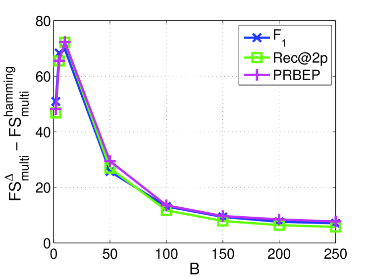
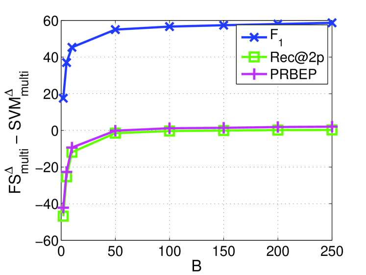
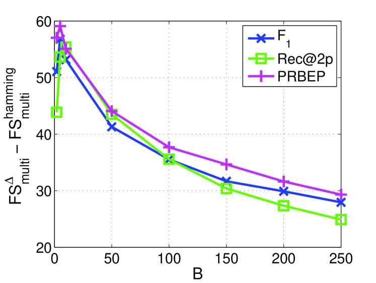
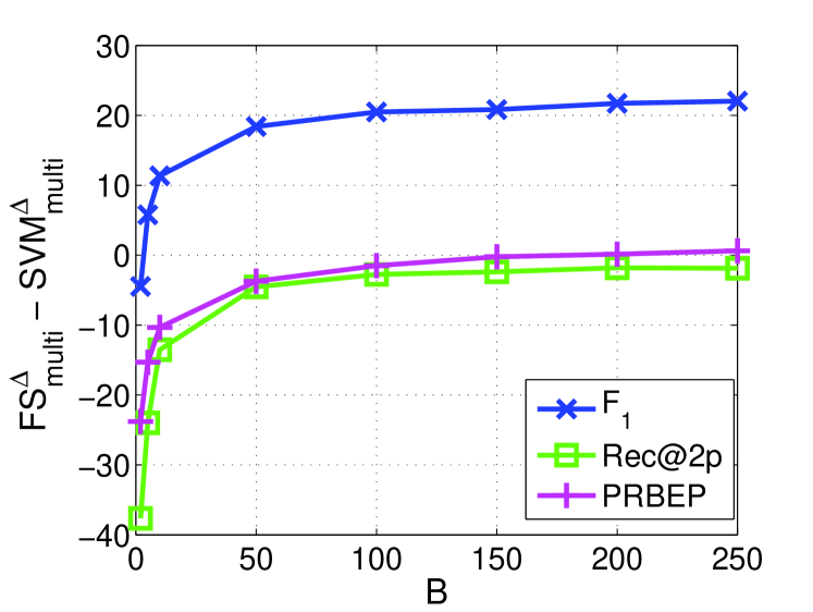
Table 2 shows the macro-average of the performance over all classes in a collection in which both and at are listed. The improvement of over and with respect to different values are reported in Figure 6. From Table 2, is consistently better than on all multivariate performance measures and two multiclass datasets. Similar results can be obtained comparing with , while the only exception is the measure Rec@2p on News20 where is a little better than . The largest gains are observed for score on all two text classification tasks. This implies that a small number of features selected by is enough to obtain comparable or even better performances for different measures than using all features.
 |
|
|---|---|
| (a) Sector | |
 |
|
| (b) News20 | |
 |
|
| (a) Sector | (b) News20 |
From Figure 6, consistently performs better than for all of the multivariate performance measures from the figures in the left-hand side. Moreover, the figures in the right-hand side show that the small number of features are good for measures, but poor for other measures. As the number of features increases, and PRBEP can approach to the results of and all curves become flat. The performance of and is relatively stable when sufficient features are selected, but our method can choose very few features for fast prediction. For measure, our method is consistently better than , and the results show significant improvement over all range of . This improvement may be due to the reduction of noisy or non-informative features. Furthermore, can achieve better performance measures than .
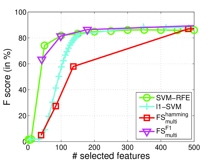
We also compared different feature selection algorithms such as SVM-RFE and -SVM on Sector and News20 in the same setting as the previous sections. The results in terms of F1 measure are reported in Figure 7. We clearly observe that outperforms -SVM on both datasets, and comparable or even better than SVM-RFE. For a small number of features, can still demonstrate very good F1 measure.
9. Conclusion
In this paper, we propose a generalized sparse regularizer for feature selection, and the unified feature selection framework for general loss functions. We particularly study in details for multivariate losses. To solve the resultant optimization problem, a two-layer cutting plane algorithm was proposed. The convergence property of the proposed algorithm is studied. Moreover, connections to a variety of state-of-the-art feature selection methods are discussed in details. A variety of analyses by comparing with the various feature selection methods show that the proposed method is superior to others. Experimental results show that the proposed method is comparable with FGM and SVM-RFE and better than models on feature selection task, and outperforms SVM for multivariate performance measures on full set of features.
Acknowledgements
This work was supported by Singapore A*star under Grant SERC 112 280 4005
Appendix A Proof of Proposition 1
Since the loss term for all , we can equivalently transform Problem
| s.t. |
into the following optimization problem
| s.t. |
By introducing a new variable and moving out summation operator from objective to be a constraint, we can obtain the equivalent optimization problem as
| s.t. | ||||
We can further simplify above problem by introducing another variables such that , , to be
| s.t. | ||||
We know that for each , is a second-order cone constraint. Following the recipe of [5], the self-dual cone can be introduced to form the Lagrangian function as follows
with dual variables , , . The derivatives of the Lagrangian with respect to the primal variables have to vanish which leads to the following KKT conditions:
By substituting all the primal variables with dual variables by above KKT conditions, we can obtain the following dual problem,
| s.t. | ||||
By setting and , we can reformulate above problem as
| s.t. |
where . According to the property of self-dual cone [3], we can obtain the primal solution from its dual as where is the dual variable of the quadratic constraint such that . By constructing Lagrangian with dual variables with respect to , we can recover Problem
| (29) |
where . This completes the proof.
Appendix B Proof of Theorem 2
Given the Problem
| (30) | or |
we have the equivalent optimization problem as
| s.t. |
The outer layer of Algorithm 2 can generate a sequence of configurations of as after iterations. In the th iteration, the most violated constraint is found in terms of , so that according to Problem . Hence, we can construct two sequences and such that
| (31) | |||||
| (32) |
Suppose that we can solve exactly. Due to the equivalence to Problem (29), it means that we can obtain the exact solution of the problem (29). Based on this assumption, equation (31) can be further reformed as
| (33) |
This turns out to be the same problem of FGM [26]. For self-completeness, we give the theorem as follows,
Theorem 3 ([26]).
Let be the globally optimal solution pair of Problem (30), sequences and have the following property
| (34) |
As increases, is monotonically increasing and is monotonically decreasing.
Based on above theorem, global optimal solution can be obtained after a finite number of iterations. However, the assumption of the accurate solution for (29) usually has no formal guarantee. We have already proven in Theorem 1 that the inner problem of Algorithm 2 can reach the desired precision after a finite number of iterations by Algorithm 1. Therefore, according to Algorithm 2, we can construct the following sequence
| (35) |
By combining inequalities (34) and (35), we obtain the following inequalities
| (36) |
After a finite number of iterations, the global optimal solution is . Hence, the solution of the Algorithm 2 may be not less than the lower bound by . It is complete for Theorem 2.
References
- [1] S. Andrews, I. Tsochantaridis, and T. Hofmann. Support vector machines for multiple-instance learning. In NIPS, 2003.
- [2] F. Bach, R. Jenatton, J. Mairal, and G. Obozinski. Optimization with sparsity-inducing penalties. Foundations and Trends in Machine Learning, 4:1–106, 2012.
- [3] F. R. Bach, G. R. G. Lanckriet, and M. I. Jordan. Multiple kernel learning, conic duality, and the SMO algorithm. In ICML, 2004.
- [4] J. M. Borwein and A. S. Lewis. Convex Analysis and Nonlinear Optimization. Springer, 2000.
- [5] S. Boyd and L. Vandenberghe. Convex Optimization. Cambridge University Press, Cambridge, UK., 2004.
- [6] Y. Chen, J. Bi, and J. Z. Wang. MILES: Multiple-instance learning via embedded instance selection. TPAMI, 28:1931–1947, 2006.
- [7] T. G. Dietterich, R. H. Lathrop, and T. Lozano-Perez. Solving the multiple instance problem with axis-parallel rectangles. Artificial Intelligence, 89:31–71, 1997.
- [8] G. M. Fung and O. L. Mangasarian. A feature selection newton method for support vector machine classification. Computational Optimization and Applications, 28:185–202, 2004.
- [9] I. Guyou, J. Weston, S. Barnhill, and V. Vapnik. Gene selection for cancer classification using support vector machines. Machine Learning, 46:389–422, 2002.
- [10] J. B. Hiriart-Urruty and C. Lemarechal. Convex Analysis and Minimization Algorithms. Springer-Verlag, 1993.
- [11] T. Joachims. A support vector method for multivariate performance measures. In ICML, 2005.
- [12] T. Joachims. Training linear SVMs in linear time. In SIGKDD, 2006.
- [13] T. Joachims, T. Finley, and C. J. Yu. Cutting-plane training of structural SVMs. Machine Learning, 77:27–59, 2009.
- [14] J. E. Kelley. The cutting plane algorithm for solving convex programs. Journal of the Society for Industrial and Applied Mathematics, 8(4):703–712, 1960.
- [15] T. N. Lal, O. Chapelle, J. Weston, and A. Elisseeff. Embedded methods. In I. Guyon, S. Gunn, M. Nikravesh, and L. A. Zadeh, editors, Feature Extraction: Foundations and Applications, Studies in Fuzziness and Soft Computing, number 207, pages 137 –165. Springer, 2006.
- [16] Q. V. Le and A. Smola. Direct optimization of ranking measures. JMLR, 1:1–48, 2007.
- [17] D. Lin, D. P. Foster, and L. H. Ungar. A risk ratio comparison of and penalized regressions. Technical report, University of Pennsylvania, 2010.
- [18] Z. Liu, F. Jiang, G. Tian, S. Wang, F. Sato, S. J. Meltzer, and M. Tan. Sparse logistic regression with penalty for biomarker identification. Statistical Applications in Genetics and Molecular Biology, 6(1), 2007.
- [19] Q. Mao and I. W. Tsang. Optimizing performance measures for feature selection. In ICDM, 2011.
- [20] O. Maron and A. L. Ratan. Multiple-instance learning for natural scene classification. In ICML, 1998.
- [21] D. R. Musicant, V. Kumar, and A. Ozgur. Optimizing f-measure with support vector machines. In Proceedings of the 16th International Florida Artificial Intelligence Research Society Conference, 2003.
- [22] A. Mutapcic and S. Boyd. Cutting-set methods for robust convex optimization with pessimizing oracles. Optimization Methods & Software, 24(3):381 406, 2009.
- [23] A. Y. Ng. Feature selection, vs. regularization, and rotational invariance. In ICML, 2004.
- [24] A. Rakotomamonjy, F. R. Bach, Y. Grandvalet, and S. Canu. SimpleMKL. JMLR, 3:1439–1461, 2008.
- [25] S. Sonnenburg, G. Rätsch, C. Schäfer, and B. Scholköpf. Large scale multiple kernel learning. JMLR, 7, 2006.
- [26] M. Tan, L. Wang, and I. W. Tsang. Learning sparse SVM for feature selection on very high dimensional datasets. In ICML, 2010.
- [27] C. H. Teo, S.V.N. Vishwanathan, A. Smola, and Quoc V. Le. Bundle methods for regularized risk minimization. JMLR, pages 311–365, 2010.
- [28] I. Tsochantaridis, T. Joachims, T. Hofmann, and Y. Altum. Large margin methods for structured and interdependent output variables. JMLR, 6:1453–1484, 2005.
- [29] H. Valizadengan, R. Jin, R. Zhang, and J. Mao. Learning to rank by optimizing ndcg measure. In NIPS, 2009.
- [30] J. Weston, A. Elisseeff, and B. Scholköpf. Use of the zero-norm with linear models and kernel methods. JMLR, 3:1439–1461, 2003.
- [31] Z. Xu, R. Jin, I. King, and M. R. Lyu. An extended level method for efficient multiple kernel learning. In NIPS, 2008.
- [32] Z. Xu, R. Jin, J. Ye, Michael R. Lyu, and I. King. Non-monotonic feature selection. In ICML, 2009.
- [33] G.-X. Yuan, K.-W. Chang, C.-J. Hsieh, and C.-J. Lin. A comparison of optimization methods and software for large-scale -regularized linear classification. JMLR, 11:3183–3234, 2010.
- [34] Y. Yue, T. Finley, F. Radlinski, and T. Joachims. A support vector method for optimizing average precision. In SIGIR, 2007.
- [35] Q. Zhang, S.A. Goldman, W. Yu, and J. Fritts. Content-based image retrieval using multiple-instance learning. In ICML, 2002.
- [36] T. Zhang. Analysis of multi-stage convex relaxation for sparse regularization. JMLR, 11:1081–1107, Mar 2010.
- [37] X. Zhang, A. Saha, and S.V.N. Vishwanathan. Smoothing multivariate performance measures. In UAI, 2011.
- [38] Z.-H. Zhou and M.-L. Zhang. Multi-instance multi-label learning with application to scene classification. In NIPS, 2007.
- [39] J. Zhu, S. Rossett, T. Hastie, and R. Tibshirani. 1-norm support vector machine. In NIPS, 2003.
- [40] A. Zien and C. S. Ong. Multiclass multiple kernel learning. In ICML, 2007.