\NewEnviron

movableProof[1][Proof] ¹¹institutetext: Amazon Robotics, North Reading, MA, USA. ¹¹email: zhangyl@amazon.com²²institutetext: Texas A&M University, College Station, TX, USA. ²²email: dshell@tamu.edu

A fixed-parameter tractable algorithm for combinatorial filter reduction

Yulin Zhang 11 Dylan A. Shell 22

Abstract

What is the minimal information that a robot must retain to achieve its task? To design economical robots, the literature dealing with reduction of combinatorial filters approaches this problem algorithmically. As lossless state compression is NP-hard, prior work has examined, along with minimization algorithms, a variety of special cases in which specific properties enable efficient solution. Complementing those findings, this paper refines the present understanding from the perspective of parameterized complexity. We give a fixed-parameter tractable algorithm for the general reduction problem by exploiting a transformation into clique covering. The transformation introduces new constraints that arise from sequential dependencies encoded within the input filter — some of these constraints can be repaired, others are treated through enumeration. Through this approach, we identify parameters affecting filter reduction that are based upon inter-constraint couplings (expressed as a notion of their height and width), which add to the structural parameters present in the unconstrained problem of minimal clique covering. Compared with existing work, we precisely identify and quantitatively characterize those features that contribute to the problem’s hardness: given a problem instance, the combinatorial core may be a fraction of the instance’s full size, with a small subset of constraints needing to be considered, and even those may have directly identifiable couplings that collapse degrees of freedom in the enumeration.

^†^†This work was done prior to Y. Zhang joining Amazon Robotics.

1 Introduction

The design of robots that are simple is important not only because small resource footprints often translate into money saved, but also because parsimony can be enlightening. In fact, the pursuit of minimalism has a long history in robotics (cf. [1, 2, 4]). But the elegance in that prior work was obtained, mostly, through human nous rather than computational tools—our work pursues the latter avenue.

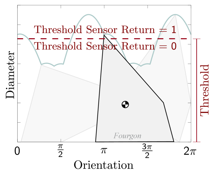
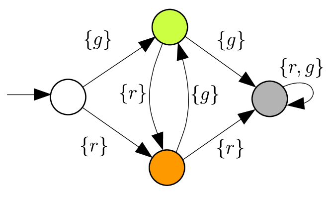
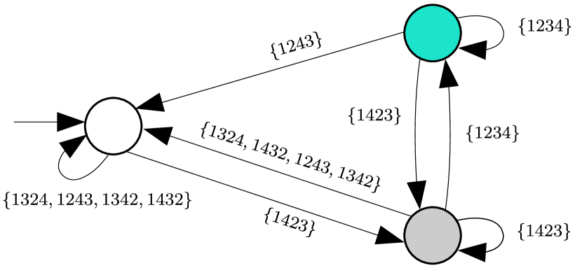
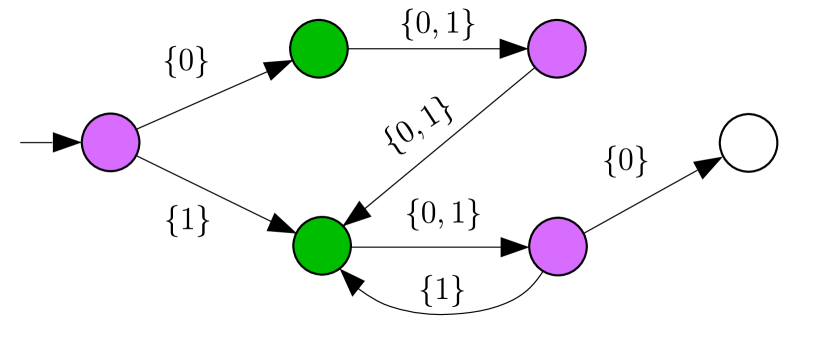
Combinatorial filters are a general and abstract model of stateful devices that take a stream of sensor readings as input and, processing sequentially, produce a stream of outputs. They have found direct application in describing estimators (e.g., tracking agents in an environment [14]) and also as representations for sensor-based plans (e.g., for navigation, or manipulation for part orientating [6]). Figure 1 provides specific concrete examples from the literature showing different scenarios and the associated filters. In the context of the present paper, what is interesting about combinatorial filters is that (unlike, say, Bayesian estimators) they are objects which themselves can be modified by algorithms. In our view, the fundamental information processing task faced by a robot can oftentimes be abstractly represented via a combinatorial filter, so specific obstructions to tractability have significance beyond mere applications; for instance, they speak to the challenge of niche fit as optimization under resource constraints.

[Uncaptioned image] — Figure 1: Diverse examples of combinatorial filters. Sakcak et al. [12] consider a circular environment like that shown in (a) with two types of break-beam sensors that trigger when crossed by an agent. They derive the 4-state filter, depicted in (b), that outputs grey when it detects that strictly clockwise/anticlockwise motion has been violated. Scenario (c) is re-drawn from [8], where the robot observes only the cyclic ordering of 4 landmarks. Their 3-state filter, depicted in (d), determines definitively whether the robot’s current location is within the cyan region. In (e), the task of orienting a polygon with a squeeze-gripper, based upon [13], is expressed as feedback plan (f), with green encoding the action of rotating the gripper by $65^{\circ}$ , and purple the squeeze action (reproduced from [18]).

1.1 Related Work

The idea of determining fundamental limits, such as necessary information and performance bounds, is a topic receiving renewed attention (for instance, see [3, 12]), especially when such analysis can be conducted via automated means. A key problem is that of taking a combinatorial filter and compressing it to form an equivalent filter, but with the fewest states. Regrettably, this is NP-hard [6]. A direction of work has sought to identify special cases [10, 19], to employ ILP and SAT techniques [7, 16], and to focus on special types of reductions which may give inexact solutions [8, 11]. (The state-of-the-art practical method for exact combinatorial filter minimization, at the time of writing, appears in [16].) The very closely related work of [10] identifies some parameters for which filter reduction is not FPT (namely: output size, treewidth, maximum number of appearances of any observation); they also give an FPT algorithm for a stage-by-stage reduction problem (not identical to the problem we study, see [17, Lemma 10, pg. 95]) which has parameters distinct from those we examine.

1.2 Contributions

The present paper gives a new fixed-parameter tractable (FPT) algorithm for the filter reduction problem. Such algorithms are so named because they involve the identification of specific parameters as dimensions that characterize problem instances as inputs to the algorithm. These algorithms have attractive (polynomial) performance when the instances are scaled up but with the parameters held constant. As a formal tool, they provide more fine-grained treatment than merely showing the problem is NP-hard [5]. The primary significance of the algorithm we introduce is that it highlights specific structural aspects of instances that make minimization difficult. Put another way: when the parameters identified are bounded, that which remains is a characterization of easy (i.e. polynomial time) filter minimization instances. For instance, easy filters to minimize are those where the number of zipper constraints (see Definition 4) is small. Or, when the set of zipper constraints might be large, minimization can be easy if the vast majority satisfy the repairability property we describe (see Definition 6), while being disconnected from those which do not. Also, when non-repairable constraints, owing to constraint inter-dependencies, form long chains, or—even better—cycles, the problem is simplified. Each of these help reduce the (worst-case) cost of solution.

The perspective we emphasize, thus, is that the algorithm provides a new complexity-theoretic insight by teasing apart specific structural factors affecting the hardness of filter reduction; though we do not put the algorithm to practical use, there is no basis to presume that it is impractical, either.

2 Preliminaries

Definition 1 (filter [9]).

A deterministic filter, or just filter, is a 6-tuple $\mathscr{F}=(V,v_{0},Y,\tau,C,c)$ , with $V$ a non-empty finite set of states, $v_{0}$ an initial state, $Y$ the set of observations, $\tau:V\times Y\hookrightarrow V$ the partial function describing transitions, $C$ the set of outputs, and $c:V\to C$ being the output function.

One traces a finite observation sequence $y_{0}y_{1}\dots y_{k}$ on a filter by starting at state $v_{0}$ , and repeatedly following the edge labeled by $y_{i}$ to arrive at $v_{i+1}=\tau(v_{i},y_{i})$ . The filter’s output is $c(v_{k})\in C$ obtained from the last state visited.

Problem: Filter Minimization ( FM $({\mathscr{F}})$ ) Input: A deterministic filter $\mathscr{F}$ . Output: A deterministic filter $\mathscr{F}^{\star}$ with fewest states, such that: 1. any sequence which can be traced on $\mathscr{F}$ can also be traced on $\mathscr{F}^{\star}$ ; 2. the outputs they produce on any of those sequences are identical. .

Solving this problem requires some minimally-sized filter $\mathscr{F}^{\star}$ that is functionally equivalent to $\mathscr{F}$ , where the notion of equivalence —called output simulation— needs only criteria 1. and 2. to be met. For a formal definition of output simulation, see [17, Definition 5, pg. 93].

Lemma 2 ([6]).

The problem FM is NP-hard.

Recently, in giving a minimization algorithm [17], FM was shown to be equivalent to vertex covering when the valid coverings satisfy a set of auxiliary constraints. These constraints, denoted ${\color[rgb]{0,0.25,0.25}\mathcal{Z}}$ , are termed zipper constraints as they may cause long chains of vertices to be ‘pulled together’ incrementally. First, we describe this vertex covering problem in and of itself. Next, this abstract problem will be connected back to filters through the notion of compatibility.

Problem: Minimum Zipped Clique Cover ( MZCC $({G},{{\color[rgb]{0,0.25,0.25}\mathcal{Z}}})$ ) Input: A graph $G=(V,E)$ and a collection of ordered pairs of $G$ ’s edges ${\color[rgb]{0,0.25,0.25}\mathcal{Z}}=\{({U_{1}};{V_{1}}),({U_{2}};{V_{2}}),\dots,({U_{m}};{V_{m}})\}$ , where $U_{i},V_{i}\in E$ . Output: Minimum cardinality clique cover $\mathbb{K}$ such that: 1. $\bigcup_{K_{i}\in\mathbb{K}}K_{i}=V$ , with each $K_{i}$ forming a clique on $G$ ; 2. $\forall K_{i}\in\mathbb{K}$ , if there is some $\ell$ such that $U_{\ell}\subseteq K_{i}$ , then some $K_{j}\in\mathbb{K}$ must have $K_{j}\supseteq V_{\ell}$ . . (This is a special case of MZCC in [17] but will suffice, see discussion in footnote 2.)

¹¹footnotetext: After examining filters like those here, the later sections of that paper go further by studying a generalization in which function

c

may be a relation. Complications arising from that generalization will not be discussed herein.

In bridging filters and covers, the key idea is that certain sets of states in a filter can be identified as candidates to merge together, and such ‘mergability’ can be expressed as a graph. The process of forming covers of this graph identifies states to consolidate and, accordingly, minimal covers yield small filters. The first technical detail concerns this graph and states that are candidates to be merged:

Definition 3 (extensions/compatibility).

For a state $v$ of filter $\mathscr{F}$ , use $\mathcal{L}_{\mathscr{F}}(v)$ to denote the set of observation sequences, or extensions, that can be traced starting from $v$ . States $v$ and $w$ are compatible if their outputs agree on $\mathcal{L}_{\mathscr{F}}(v)\cap\mathcal{L}_{\mathscr{F}}(w)$ , their common extensions. In such cases, we write $v\sim_{c}w$ . The compatibility graph $G_{\mathscr{F}}$ possesses edges between states if and only if they are compatible.

But simply building a minimal cover on $G_{\mathscr{F}}$ is not enough because covers may merge some elements which, when transformed into a filter, produce nondeterminism. The core obstruction is when a fork is created, as when two compatible states are merged, both of which have outgoing edges bearing identical labels, but whose destinations differ. To enforce determinism, we use constraints to forbid forking and require mergers to flow downwards. See the following:

Definition 4 (determinism-enforcing zipper constraints).

Given a pair of compatible states $U=\{u_{1},u_{2}\}$ in $\mathscr{F}$ and their $y$ -children, $V=\{\tau(u_{1},y),\tau(u_{2},y)\}$ , then the ordered pair $({U};{V})$ is a determinism-enforcing zipper constraint of $\mathscr{F}$ .

A zipper constraint $({U};{V})$ is satisfied by a clique cover if $U$ is not covered in a clique, or both $U$ and $V$ are covered in cliques. (This is criterion 2. for MZCC .) For filters, in other words, if the states in $U$ are to be merged (or consolidated) then the downstream states, in $V$ , must be as well. 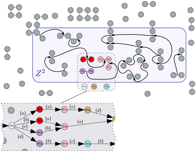The collection of all determinism-enforcing zipper constraints for a filter $\mathscr{F}$ is denoted ${\color[rgb]{0,0.25,0.25}\mathcal{Z}}_{\mathscr{F}}$ .

Refer to caption — Figure 2: An illustration showing (partially) a filter $\mathscr{F}$ (left inset) leading to a compatibility graph $G_{\mathscr{F}}$ (above). The ${Z^{2}}$ set is also shown.

In summary: for filter $\mathscr{F}$ , the collection of zipper constraints ${\color[rgb]{0,0.25,0.25}\mathcal{Z}}_{\mathscr{F}}$ that ensures the desired result will be a deterministic filter can be constructed directly as follows. For $u\sim_{c}v$ , a pair of compatible states in $\mathscr{F}$ , use $\tau(\cdot,y)$ to trace forward under observation $y$ ; if the $y$ -children thus obtained are distinct, we form zipper constraint $(\{u,v\},\{\tau(u,y),\tau(v,y)\})$ to ensure that if $u$ and $v$ are merged (by occupying some set in the cover together), their $y$ -children will be as well. Construct ${\color[rgb]{0,0.25,0.25}\mathcal{Z}}_{\mathscr{F}}$ by collecting all such constraints for all compatible pairs, using every observation. A cartoon illustrating the result of this procedure is shown in Figure 2: a snippet of the filter $\mathscr{F}$ appears at bottom left; its undirected compatibility graph, $G_{\mathscr{F}}$ , appears above; zipper constraints are shown as the directed edges on the undirected compatibility edges. Both $G_{\mathscr{F}}$ and ${\color[rgb]{0,0.25,0.25}\mathcal{Z}}_{\mathscr{F}}$ are clearly polynomial in the size of $\mathscr{F}$ . Then, a minimizer of $\mathscr{F}$ can be obtained from the solution to the minimum zipped vertex cover problem, MZCC $({G_{\mathscr{F}}},{{\color[rgb]{0,0.25,0.25}\mathcal{Z}}_{\mathscr{F}}})$ :

Lemma 5 ([17]).

Any FM $({\mathscr{F}})$ can be converted to an MZCC $({G_{\mathscr{F}}},{{\color[rgb]{0,0.25,0.25}\mathcal{Z}}_{\mathscr{F}}})$ in polynomial time; hence MZCC is NP-hard.

Though we skip the details, the proof in [17] of the preceding lemma also gives an efficient way to construct a deterministic filter from the minimum cardinality clique cover.

As a final point on the connection of these two problems, combinatorial filters generate ‘most’ graphs. Specifically, [19] proves that some filter $\mathscr{F}$ realizes $G$ as its constraint graph $G_{\mathscr{F}}$ if and only if either: (1) the graph $G$ has at least two connected components, or (2) $G$ is a complete graph.

In any graph $G=(V,E)$ , we refer to the neighbors of a vertex $v\in V$ by set $\mathcal{N}_{G}(v)\coloneqq\{w\in V\;|\;(w,v)\in E\}\cup\{v\}$ . Note that we explicitly include $v$ in its own neighborhood.

Definition 6 (comparable neighborhoods ²²2This generalizes a concept first introduced in [19, Definition 25].).

A pair of vertices $\{{v},{w}\}$ in some graph $G=(V,E)$ have comparable neighborhoods if and only if we have either $\mathcal{N}_{G}(v)\subseteq\mathcal{N}_{G}(w)$ or $\mathcal{N}_{G}(v)\supseteq\mathcal{N}_{G}(w)$ .

We will use the following recent result of Ullah:

Lemma 7 (From [15]).

Given a graph $G$ with $n$ vertices, let $\beta$ be the size of the largest clique in $G$ , and let the number of cliques in the minimum clique cover be $m$ , then there is an algorithm that computes the minimum clique cover in $2^{\beta m\log m}\,n^{O(1)}$ .

Proof.

This follows from Theorem 1.8 of [15, pg. 4], and the algorithms therein: in his notation, we solve a VCC problem, which is possible via the LRCC problem with its three parameters set to $G$ , $k=m$ , $E^{*}=\varnothing$ . ∎

3 Zippers and prescriptions

For a zipper constraint collection ${\color[rgb]{0,0.25,0.25}\mathcal{Z}}=\{({U_{1}};{V_{1}}),({U_{2}};{V_{2}}),\dots,({U_{m}};{V_{m}})\}$ , let ${Z^{2}}=\{U_{1},U_{2},\dots,U_{m},V_{1},V_{2},\dots,V_{m}\}$ , i.e., the unordered pairs of vertices (or edges) appearing within collection ${\color[rgb]{0,0.25,0.25}\mathcal{Z}}$ . We will write $P\mathrlap{\raisebox{1.0pt}{${}^{\,\phantom{\ast}}$}}{\,\prec\,}Q$ if and only if there exists a zipper constraint $({P};{Q})\in{\color[rgb]{0,0.25,0.25}\mathcal{Z}}$ . We define $Z_{\scalebox{0.5}{\text{src}}}^{2}\subseteq{Z^{2}}$ to be the set $Z_{\scalebox{0.5}{\text{src}}}^{2}\coloneqq\{P\subseteq V(\mathscr{F})\;|\;\exists Q\in{Z^{2}},P\mathrlap{\raisebox{1.0pt}{${}^{\,\phantom{\ast}}$}}{\,\prec\,}Q\}$ , i.e., the unordered pairs appearing as sources in the zipper constraint collection ${\color[rgb]{0,0.25,0.25}\mathcal{Z}}$ . Similarly, let $Z_{\scalebox{0.5}{\text{tgt}}}^{2}\subseteq{Z^{2}}$ be those pairs appearing as potential targets for enforced merging within the zipper constraints, i.e., $Z_{\scalebox{0.5}{\text{tgt}}}^{2}\coloneqq\{Q\subseteq V(\mathscr{F})\;|\;\exists P\in{Z^{2}},P\mathrlap{\raisebox{1.0pt}{${}^{\,\phantom{\ast}}$}}{\,\prec\,}Q\}$ . By construction ${Z^{2}}=Z_{\scalebox{0.5}{\text{src}}}^{2}\cup Z_{\scalebox{0.5}{\text{tgt}}}^{2}$ , and, in general, $Z_{\scalebox{0.5}{\text{src}}}^{2}\cap Z_{\scalebox{0.5}{\text{tgt}}}^{2}\neq\varnothing$ .

Definition 8.

Given ${\color[rgb]{0,0.25,0.25}\mathcal{Z}}$ , the pair $P_{b}\in{Z^{2}}$ is downstream from pair $P_{a}\in{Z^{2}}$ , written $P_{a}\mathrlap{\raisebox{1.0pt}{${}^{\,\ast}$}}{\,\prec\,}P_{b}$ , if $P_{a}\mathrlap{\raisebox{1.0pt}{${}^{\,\phantom{\ast}}$}}{\,\prec\,}P_{b}$ , or if $P_{a}\mathrlap{\raisebox{1.0pt}{${}^{\,\phantom{\ast}}$}}{\,\prec\,}P_{c}$ for some $P_{c}\in{Z^{2}}$ with $P_{c}\mathrlap{\raisebox{1.0pt}{${}^{\,\ast}$}}{\,\prec\,}P_{b}$ .

3.1 Prescriptions

To tackle the MZCC problem, we search for covers subject to a rule stating that some specific pairs must be merged, while others must never be. The idea is to make and fix choices for a subset of the pairs involved in the zipper constraint collection so that this prescription respects the zipper constraints for elements in the collection. We will denote the collection via set ${\color[rgb]{0.0,0.0,0.4}D}$ , defined next.

Definition 9.

With zipper constraint collection ${\color[rgb]{0,0.25,0.25}\mathcal{Z}}$ given some set of pairs ${\color[rgb]{0.0,0.0,0.4}D}\subseteq{Z^{2}}$ , a prescription on ${\color[rgb]{0.0,0.0,0.4}D}$ is a subset of pairs $\mathbb{S}^{\scalebox{0.5}{\text{ON}}}_{{\color[rgb]{0.0,0.0,0.4}D}}\subseteq{\color[rgb]{0.0,0.0,0.4}D}$ . 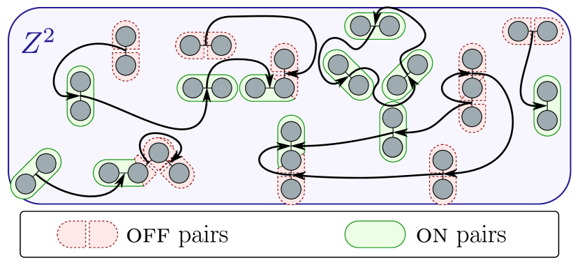Prescription $\mathbb{S}^{\scalebox{0.5}{\text{ON}}}_{{\color[rgb]{0.0,0.0,0.4}D}}$ on ${\color[rgb]{0.0,0.0,0.4}D}$ is termed downstream enabled if and only if $(P_{a}\in\mathbb{S}^{\scalebox{0.5}{\text{ON}}}_{{\color[rgb]{0.0,0.0,0.4}D}})\wedge(P_{a}\mathrlap{\raisebox{1.0pt}{${}^{\,\ast}$}}{\,\prec\,}P_{b})\implies(P_{b}\in\mathbb{S}^{\scalebox{0.5}{\text{ON}}}_{{\color[rgb]{0.0,0.0,0.4}D}})\vee(P_{b}\not\in{\color[rgb]{0.0,0.0,0.4}D})$ .

The elements in $\mathbb{S}^{\scalebox{0.5}{\text{ON}}}_{{\color[rgb]{0.0,0.0,0.4}D}}$ are called the on pairs; those in ${\color[rgb]{0.0,0.0,0.4}D}\setminus\mathbb{S}^{\scalebox{0.5}{\text{ON}}}_{{\color[rgb]{0.0,0.0,0.4}D}}$ are the off pairs, which we write as $\mathbb{S}^{\scalebox{0.5}{\text{OFF}}}_{{\color[rgb]{0.0,0.0,0.4}D}}$ . A prescription is silent about elements outside ${\color[rgb]{0.0,0.0,0.4}D}$ (the mnemonic for ${\color[rgb]{0.0,0.0,0.4}D}$ being ‘domain’ — elements within the domain are prescribed as either being on or off; elements outside the domain have no prescription). See Figure 3. (Note that since ${\color[rgb]{0.0,0.0,0.4}D}\subseteq{Z^{2}}$ , both the on pairs and off pairs are from the set of zipper constraints, hence are edges within the graph in the MZCC problem.) If $\mathbb{S}^{\scalebox{0.5}{\text{ON}}}_{{\color[rgb]{0.0,0.0,0.4}D}}=\{P_{1},P_{2},\dots,P_{m}\}$ is a prescription, then it will be used to require that the on pairs be merged, while the off pairs are prohibited from being merged. The idea is to ensure that a cover is produced that respects the prescription:

Definition 10 (Faithfulness).

Let graph $G$ and the collection of zipper constraints ${\color[rgb]{0,0.25,0.25}\mathcal{Z}}$ be given. For some domain ${\color[rgb]{0.0,0.0,0.4}D}\subseteq{Z^{2}}$ , a cover $\mathbb{K}=\{K_{1},K_{2},\allowbreak\dots,K_{m}\}$ of $G$ is faithful to prescription $\mathbb{S}^{\scalebox{0.5}{\text{ON}}}_{{\color[rgb]{0.0,0.0,0.4}D}}=\{P_{1},P_{2},\dots,P_{n}\}$ if and only if:

1.

For every $P_{i}\in\mathbb{S}^{\scalebox{0.5}{\text{ON}}}_{{\color[rgb]{0.0,0.0,0.4}D}}$ there exists some clique $K_{\ell}\in\mathbb{K}$ where $P_{i}\subseteq K_{\ell}$ ;
2.

For every $P_{j}\in\mathbb{S}^{\scalebox{0.5}{\text{OFF}}}_{{\color[rgb]{0.0,0.0,0.4}D}}$ there is no clique $K_{\ell}\in\mathbb{K}$ such that $P_{j}\subseteq K_{\ell}$ .

We will achieve this via modification of a compatibility graph that will make on and off sets enforce and prohibit mergers. The modification of the graph is given through a series of set constructions next, before showing (in Lemma 17) that this can be used as desired.

3.2 Enumerating downstream enabled prescriptions

A pair graph is a directed graph whose vertices are pairs from ${\color[rgb]{0.0,0.0,0.4}D}$ . We will write $\mathbb{G}$ , where vertices $\mathbb{V}(\mathbb{G})\subseteq{\color[rgb]{0.0,0.0,0.4}D}$ and edges $\mathbb{E}(\mathbb{G})\subseteq\mathbb{V}(\mathbb{G})\times\mathbb{V}(\mathbb{G})$ . Let $\mathbb{G}-[R]$ denote the subgraph $\mathbb{G^{\prime}}$ with vertices $R$ removed, i.e., vertices $\mathbb{V}(\mathbb{G^{\prime}})=\mathbb{V}(\mathbb{G})\setminus R$ , and also edges $\mathbb{E}(\mathbb{G^{\prime}})=\left(\mathbb{V}(\mathbb{G^{\prime}})\times\mathbb{V}(\mathbb{G^{\prime}})\right)\cap\mathbb{E}(\mathbb{G})$ . Next, we define the collection of up and downstream pairs within a given pair graph: $\mathcal{U}_{\mathbb{G}}({P})\!=\!\{P_{u}\in\mathbb{V}(\mathbb{G})\!\mid\!P_{u}\mathrlap{\raisebox{1.0pt}{${}^{\,\ast}$}}{\,\prec\,}P\}$ ; $\mathcal{D}_{\mathbb{G}}({P})\!=\!\{P_{d}\in\mathbb{V}(\mathbb{G})\!\mid\!P\mathrlap{\raisebox{1.0pt}{${}^{\,\ast}$}}{\,\prec\,}P_{d}\}.$

Algorithm 1 EnumDS(

\mathbb{G}

)

0: Pair graph

\mathbb{G}

0: All prescriptions that are downstream enabled

1: if

\mathbb{V}(\mathbb{G})=\varnothing

then

2: return

\;\varnothing

3: Let

P\in\mathbb{V}(\mathbb{G})

be an arbitrary pair where

\forall Q\in\mathbb{V}(\mathbb{G})

|\mathcal{D}_{\mathbb{G}}({P})|\geq|\mathcal{D}_{\mathbb{G}}({Q})|

4: return

\;\;{\color[rgb]{0.375,0,0.125}\textrm{{EnumDS}}}\big{(}\mathbb{G}-[\mathcal{U}_{\mathbb{G}}({P})]\big{)}\bigcup\Big{\{}\!\{P\}\cup\mathcal{D}_{\mathbb{G}}({P})\cup S\,\big{|}\,S\in{\color[rgb]{0.375,0,0.125}\textrm{{EnumDS}}}\big{(}\mathbb{G}-[\mathcal{D}_{\mathbb{G}}({P})]\big{)}\!\Big{\}}

To generate all downstream enabled prescriptions, we invoke EnumDS( $\mathbb{G}$ ( ${\color[rgb]{0.0,0.0,0.4}D}$ )) in Algorithm 1, where $\mathbb{G}({\color[rgb]{0.0,0.0,0.4}D})$ is the pair graph having vertices ${\color[rgb]{0.0,0.0,0.4}D}$ , and an edge from pair $P_{s}$ to $P_{d}$ if and only if $P_{s}\mathrlap{\raisebox{1.0pt}{${}^{\,\phantom{\ast}}$}}{\,\prec\,}P_{d}$ . In the return statement in line 4, the first set corresponds to prescriptions where $P$ is being turned off, while the second set has $P$ being turned on. Note that because cycles are possible between zipper constraints, $\mathcal{U}_{\mathbb{G}}({P})\cap\mathcal{D}_{\mathbb{G}}({P})\neq\varnothing$ , in general. The presence of cycles reduces the number of prescriptions to enumerate. When $P$ appears within a cycle, if $P$ is off, then all pairs in the cycle have to be off too; if $P$ in on, then they are all also on as well.

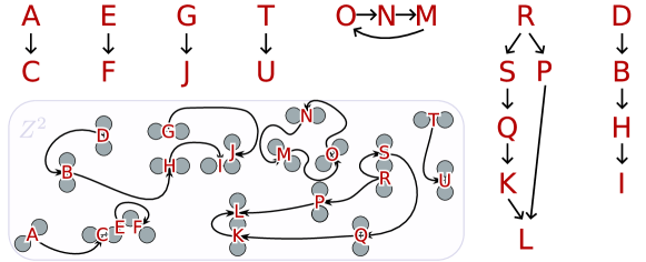
To dispatch with cycles, define a relation on pairs in ${\color[rgb]{0.0,0.0,0.4}D}$ : let $P\equiv Q$ if and only if $P=Q$ or $P\mathrlap{\raisebox{1.0pt}{${}^{\,\ast}$}}{\,\prec\,}Q\mathrlap{\raisebox{1.0pt}{${}^{\,\ast}$}}{\,\prec\,}P$ . Further, $\equiv$ is an equivalence relation and the set of equivalence classes ${\color[rgb]{0.0,0.0,0.4}D}/\!\!\!\equiv$ can be partially ordered by lifting the $\mathrlap{\raisebox{1.0pt}{${}^{\,\ast}$}}{\,\prec\,}$ relation. Then the total number of downstream enabled prescriptions, $|{\color[rgb]{0.375,0,0.125}\textrm{{EnumDS}}}(\mathbb{G})|$ , is bounded by $((\ell+1)+1)^{\omega}=2^{\omega\lg(2+\ell)}$ with $\ell$ being the height (i.e., the length of the longest chain) and $\omega$ width (i.e., size of the largest anti-chain) of $({\color[rgb]{0.0,0.0,0.4}D}/\!\!\equiv,\mathrlap{\raisebox{1.0pt}{${}^{\,\ast}$}}{\,\prec\,})$ respectively. See Figure 4 above.

As the enumeration is of downstream-enabled prescriptions from ${Z^{2}}$ , it is worth noting, firstly, that ${Z^{2}}$ will often be much smaller than the size of the input filter ( $|{Z^{2}}|\leq|V(\mathscr{F})|$ ). Second, ${\color[rgb]{0.0,0.0,0.4}D}$ may be a proper subset of ${Z^{2}}$ (see Section 6, where $|{\color[rgb]{0.0,0.0,0.4}D}|\leq|{Z^{2}}|$ ). Third, the number of downstream-enabled prescriptions for ${\color[rgb]{0.0,0.0,0.4}D}$ will often be much smaller than $2^{|{\color[rgb]{0.0,0.0,0.4}D}|}$ , i.e., $\omega\ll|{\color[rgb]{0.0,0.0,0.4}D}|$ , owing to both the reduction obtained from cycles ( $|{\color[rgb]{0.0,0.0,0.4}D}/\!\!\equiv\!|\leq|{\color[rgb]{0.0,0.0,0.4}D}|$ ), and ordering structure inherited from the sequential zipping that arises from the filter (e.g., as $\ell$ increases, worst-case $\omega$ decreases).

4 Graph Augmentation

Downstream-enabled prescriptions are effective at encoding choices that are imperative to satisfaction of the zipper constraints, without specifying a full clique cover. Given such a prescription, first we augment the compatibility graph by incorporating the prescription. Thereafter, as the zipper constraints are no longer a concern, we can focus on the remaining minimum clique cover problem on the augmented graph. Finally we transport the solution from the augmented graph back to the original compatibility graph.

4.1 Augmenting the constraint graph

Construction 11 (Augmented Graph $G^{+}$ ).

If $G=(V,E)$ , then construct $G^{+}(\mathbb{S}^{\scalebox{0.5}{\text{ON}}}_{{\color[rgb]{0.0,0.0,0.4}D}})=\left(V^{+}(\mathbb{S}^{\scalebox{0.5}{\text{ON}}}_{{\color[rgb]{0.0,0.0,0.4}D}}),E^{+}(\mathbb{S}^{\scalebox{0.5}{\text{ON}}}_{{\color[rgb]{0.0,0.0,0.4}D}})\right)$ with $V^{+}(\mathbb{S}^{\scalebox{0.5}{\text{ON}}}_{{\color[rgb]{0.0,0.0,0.4}D}})\coloneqq V_{{\scalebox{0.7}{\text{prior}}}}\cup V_{{\scalebox{0.7}{\text{new}}}}(\mathbb{S}^{\scalebox{0.5}{\text{ON}}}_{{\color[rgb]{0.0,0.0,0.4}D}})$ where

$V_{{\scalebox{0.7}{\text{prior}}}}\coloneqq\big{\{}\mathsf{v}_{{\scalebox{0.7}{\text{new}}}}^{\scalebox{0.67}{$\!\{{u}\}\!$}}\;\big{|}\;u\in V\big{\}}$ ,
$V_{{\scalebox{0.7}{\text{new}}}}(\mathbb{S}^{\scalebox{0.5}{\text{ON}}}_{{\color[rgb]{0.0,0.0,0.4}D}})\coloneqq\big{\{}\mathsf{v}_{{\scalebox{0.7}{\text{new}}}}^{\scalebox{0.67}{$\!\{{u},{w}\}\!$}}\;\big{|}\;\{{u},{w}\}\in\mathbb{S}^{\scalebox{0.5}{\text{ON}}}_{{\color[rgb]{0.0,0.0,0.4}D}}\big{\}}$ ,
$E^{+}(\mathbb{S}^{\scalebox{0.5}{\text{ON}}}_{{\color[rgb]{0.0,0.0,0.4}D}})\coloneqq\Big{\{}\{{\mathsf{v}_{{\scalebox{0.7}{\text{new}}}}^{\scalebox{0.67}{${A}$}}},{\mathsf{v}_{{\scalebox{0.7}{\text{new}}}}^{\scalebox{0.67}{${B}$}}}\}\in V^{+}(\mathbb{S}^{\scalebox{0.5}{\text{ON}}}_{{\color[rgb]{0.0,0.0,0.4}D}})\times V^{+}(\mathbb{S}^{\scalebox{0.5}{\text{ON}}}_{{\color[rgb]{0.0,0.0,0.4}D}})\;\Big{|}\;A\cup B\text{ form a clique in}\phantom{xxx}\allowbreak\phantom{.}\hfill\text{graph }G^{\prime}=(V,E\setminus\mathbb{S}^{\scalebox{0.5}{\text{OFF}}}_{{\color[rgb]{0.0,0.0,0.4}D}})\Big{\}}$ .

The vertices in $V_{\scalebox{0.7}{\text{prior}}}$ are simply re-named copies of those in $V$ . The set $V_{{\scalebox{0.7}{\text{new}}}}$ introduces new vertices for those pairs in ${\color[rgb]{0.0,0.0,0.4}D}$ which have been turned on. The definition of the edge set adds edges to ensure that the new vertices will be seen as mutually compatible when there is no obstruction to compatibility from within the original graph.

Property 12.

Let vertices $\mathsf{v}_{{\scalebox{0.7}{\text{new}}}}^{\scalebox{0.67}{${A}$}},\mathsf{v}_{{\scalebox{0.7}{\text{new}}}}^{\scalebox{0.67}{${B}$}}\in V^{+}(\mathbb{S}^{\scalebox{0.5}{\text{ON}}}_{{\color[rgb]{0.0,0.0,0.4}D}})$ , $\mathsf{v}_{{\scalebox{0.7}{\text{new}}}}^{\scalebox{0.67}{${A}$}}\neq\mathsf{v}_{{\scalebox{0.7}{\text{new}}}}^{\scalebox{0.67}{${B}$}}$ then

\{\mathsf{v}_{{\scalebox{0.7}{\text{new}}}}^{\scalebox{0.67}{${A}$}},\mathsf{v}_{{\scalebox{0.7}{\text{new}}}}^{\scalebox{0.67}{${B}$}}\}\in E^{+}(\mathbb{S}^{\scalebox{0.5}{\text{ON}}}_{{\color[rgb]{0.0,0.0,0.4}D}})\iff\forall u\in A,\forall w\in B,u\neq w,\{\mathsf{v}_{{\scalebox{0.7}{\text{new}}}}^{\scalebox{0.67}{$\!\{{u}\}\!$}},\mathsf{v}_{{\scalebox{0.7}{\text{new}}}}^{\scalebox{0.67}{$\!\{{w}\}\!$}}\}\in E^{+}(\mathbb{S}^{\scalebox{0.5}{\text{ON}}}_{{\color[rgb]{0.0,0.0,0.4}D}}).

Proof.

When $A$ and $B$ are singletons, i.e., $\mathsf{v}_{{\scalebox{0.7}{\text{new}}}}^{\scalebox{0.67}{${A}$}},\mathsf{v}_{{\scalebox{0.7}{\text{new}}}}^{\scalebox{0.67}{${B}$}}\in V{\scalebox{0.7}{\text{prior}}}$ , the two sides of the if and only if are identical statements.

$\impliedby$

The given antecedents and fact that $\mathsf{v}_{{\scalebox{0.7}{\text{new}}}}^{\scalebox{0.67}{${A}$}},\mathsf{v}_{{\scalebox{0.7}{\text{new}}}}^{\scalebox{0.67}{${B}$}}\in V^{+}(\mathbb{S}^{\scalebox{0.5}{\text{ON}}}_{{\color[rgb]{0.0,0.0,0.4}D}})$ are exactly the conditions in the construction of $E^{+}(\mathbb{S}^{\scalebox{0.5}{\text{ON}}}_{{\color[rgb]{0.0,0.0,0.4}D}})$ , hence $\{\mathsf{v}_{{\scalebox{0.7}{\text{new}}}}^{\scalebox{0.67}{${A}$}},\mathsf{v}_{{\scalebox{0.7}{\text{new}}}}^{\scalebox{0.67}{${B}$}}\}\in E^{+}(\mathbb{S}^{\scalebox{0.5}{\text{ON}}}_{{\color[rgb]{0.0,0.0,0.4}D}})$ .
$\implies$

Suppose $\{\mathsf{v}_{{\scalebox{0.7}{\text{new}}}}^{\scalebox{0.67}{${A}$}},\mathsf{v}_{{\scalebox{0.7}{\text{new}}}}^{\scalebox{0.67}{${B}$}}\}\in E^{+}(\mathbb{S}^{\scalebox{0.5}{\text{ON}}}_{{\color[rgb]{0.0,0.0,0.4}D}})$ but there is some $u\in A$ and $w\in B$ with $\{\mathsf{v}_{{\scalebox{0.7}{\text{new}}}}^{\scalebox{0.67}{$\!\{{u}\}\!$}},\mathsf{v}_{{\scalebox{0.7}{\text{new}}}}^{\scalebox{0.67}{$\!\{{w}\}\!$}}\}\not\in E^{+}(\mathbb{S}^{\scalebox{0.5}{\text{ON}}}_{{\color[rgb]{0.0,0.0,0.4}D}})$ . Since $u\neq w$ , hence $\{u,w\}\not\in E$ or $\{u,w\}\in\mathbb{S}^{\scalebox{0.5}{\text{OFF}}}_{{\color[rgb]{0.0,0.0,0.4}D}}$ ; both contradict the supposition that $\{\mathsf{v}_{{\scalebox{0.7}{\text{new}}}}^{\scalebox{0.67}{${A}$}},\mathsf{v}_{{\scalebox{0.7}{\text{new}}}}^{\scalebox{0.67}{${B}$}}\}\in E^{+}(\mathbb{S}^{\scalebox{0.5}{\text{ON}}}_{{\color[rgb]{0.0,0.0,0.4}D}})$ .

∎

4.2 Relating graphs and their augmentations

Next, we consider two operations which connect vertices in the original graph with those in its augmented graph.

Definition 13 (Distillation).

Suppose a graph $G=(V,E)$ and its augmentation $G^{+}(\mathbb{S}^{\scalebox{0.5}{\text{ON}}}_{{\color[rgb]{0.0,0.0,0.4}D}})$ based on prescription $\mathbb{S}^{\scalebox{0.5}{\text{ON}}}_{{\color[rgb]{0.0,0.0,0.4}D}}\subseteq{\color[rgb]{0.0,0.0,0.4}D}$ is given. The set of vertices of the augmented graph, $S^{+}=\{\mathsf{v}_{{\scalebox{0.7}{\text{new}}}}^{\scalebox{0.67}{${A_{1}}$}},\mathsf{v}_{{\scalebox{0.7}{\text{new}}}}^{\scalebox{0.67}{${A_{2}}$}},\dots,\mathsf{v}_{{\scalebox{0.7}{\text{new}}}}^{\scalebox{0.67}{${A_{n}}$}}\}\subseteq V^{+}(\mathbb{S}^{\scalebox{0.5}{\text{ON}}}_{{\color[rgb]{0.0,0.0,0.4}D}})$ , may be distilled to obtain a set of vertices in the original graph: $S\coloneqq A_{1}\cup A_{2}\cup\dots\cup A_{n}.$

In the preceding, when $S$ is obtained from $S^{+}$ in this way, we will also refer to it as $S^{+}$ ’s distillate. Further, we will also talk of the distillate of a collection of sets $\{S_{1}^{+},S_{2}^{+},\dots,S_{n}^{+}\}$ , as the collection obtained by applying Definition 13 to each $S_{i}^{+}$ , each yielding their respective $S_{i}$ . In the particular uses of this concept which follow we will be interested in distilling collections that are covers. The next property shows that distillation preserves cliqueness, while transporting a structure from graph $G^{+}$ back to $G$ .

Property 14.

For a graph $G=(V,E)$ and its augmentation $G^{+}(\mathbb{S}^{\scalebox{0.5}{\text{ON}}}_{{\color[rgb]{0.0,0.0,0.4}D}})$ based on prescription $\mathbb{S}^{\scalebox{0.5}{\text{ON}}}_{{\color[rgb]{0.0,0.0,0.4}D}}\subseteq{\color[rgb]{0.0,0.0,0.4}D}$ , suppose $S^{+}\subseteq V^{+}(\mathbb{S}^{\scalebox{0.5}{\text{ON}}}_{{\color[rgb]{0.0,0.0,0.4}D}})$ produces $S\subseteq V$ when distilled. Then $S^{+}$ is a clique in $G^{+}(\mathbb{S}^{\scalebox{0.5}{\text{ON}}}_{{\color[rgb]{0.0,0.0,0.4}D}})$ if and only if $S$ is a clique in $G^{\prime}=(V,E\setminus(\mathbb{S}^{\scalebox{0.5}{\text{OFF}}}_{{\color[rgb]{0.0,0.0,0.4}D}}))$ .

Proof.

$\impliedby:$ Let $S^{+}=\{\mathsf{v}_{{\scalebox{0.7}{\text{new}}}}^{\scalebox{0.67}{${A_{1}}$}},\mathsf{v}_{{\scalebox{0.7}{\text{new}}}}^{\scalebox{0.67}{${A_{2}}$}},\dots,\mathsf{v}_{{\scalebox{0.7}{\text{new}}}}^{\scalebox{0.67}{${A_{n}}$}}\}$ . According to Construction 11, for every $\mathsf{v}_{{\scalebox{0.7}{\text{new}}}}^{\scalebox{0.67}{${A_{i}}$}}$ and $\mathsf{v}_{{\scalebox{0.7}{\text{new}}}}^{\scalebox{0.67}{${A_{j}}$}}$ , with $i\neq j$ , we know that $A_{i}\cup A_{j}$ form a clique in $G^{\prime}$ . But $A_{i}\cup A_{j}\subseteq S$ ; since $S$ is a clique, $A_{i}\cup A_{j}$ is a clique, and hence there is an edge in $E^{+}(\mathbb{S}^{\scalebox{0.5}{\text{ON}}}_{{\color[rgb]{0.0,0.0,0.4}D}})$ connecting $\mathsf{v}_{{\scalebox{0.7}{\text{new}}}}^{\scalebox{0.67}{${A_{i}}$}}$ and $\mathsf{v}_{{\scalebox{0.7}{\text{new}}}}^{\scalebox{0.67}{${A_{j}}$}}$ .

$\implies:$ Suppose $S$ was not a clique, then there are distinct vertices $u,w\in S$ that have no connecting edge in $G^{\prime}$ . But $S$ being the distillate of $S^{+}$ means that there is some $\mathsf{v}_{{\scalebox{0.7}{\text{new}}}}^{\scalebox{0.67}{${A_{u}}$}}\in S^{+}$ with $u\in A_{u}$ , and some $\mathsf{v}_{{\scalebox{0.7}{\text{new}}}}^{\scalebox{0.67}{${A_{w}}$}}\in S^{+}$ with $w\in A_{w}$ . If $A_{u}=A_{w}=\{{u},{w}\}$ , then $\mathsf{v}_{{\scalebox{0.7}{\text{new}}}}^{\scalebox{0.67}{$\!\{{u},{w}\}\!$}}\in V_{{\scalebox{0.7}{\text{new}}}}(\mathbb{S}^{\scalebox{0.5}{\text{ON}}}_{{\color[rgb]{0.0,0.0,0.4}D}})$ , but that implies $\{{u},{w}\}\in\mathbb{S}^{\scalebox{0.5}{\text{ON}}}_{{\color[rgb]{0.0,0.0,0.4}D}}\subseteq E\setminus\mathbb{S}^{\scalebox{0.5}{\text{OFF}}}_{{\color[rgb]{0.0,0.0,0.4}D}}$ , a contradiction. Otherwise, $A_{u}\neq A_{v}$ but this is also a contradiction for we know $S^{+}$ is a clique, so there is an edge between $\mathsf{v}_{{\scalebox{0.7}{\text{new}}}}^{\scalebox{0.67}{${A_{u}}$}}$ and $\mathsf{v}_{{\scalebox{0.7}{\text{new}}}}^{\scalebox{0.67}{${A_{w}}$}}$ , but Construction 11, thus, requires an edge between $u$ and $w$ in $G^{\prime}$ . ∎

The concept in the following definition is a sort of counterpoint to that of Definition 13.

Definition 15 (Expansion).

{\operatorname{expand}}({S})\coloneqq\{\mathsf{v}_{{\scalebox{0.7}{\text{new}}}}^{\scalebox{0.67}{${A}$}}\in V^{+}(\mathbb{S}^{\scalebox{0.5}{\text{ON}}}_{{\color[rgb]{0.0,0.0,0.4}D}})\mid A\subseteq S\}.

(1)

(Notice the subtlety that binding elements to within $V^{+}(\mathbb{S}^{\scalebox{0.5}{\text{ON}}}_{{\color[rgb]{0.0,0.0,0.4}D}})$ ensures $A$ will be singletons or pairs.) Observe that if $S^{+}={\operatorname{expand}}({S})$ , i.e. $S$ expands to $S^{+}$ , then the distillation of $S^{+}$ is $S$ — this is proved as the first part of the next property.

Property 16.

Given a graph $G=(V,E)$ and its augmentation $G^{+}(\mathbb{S}^{\scalebox{0.5}{\text{ON}}}_{{\color[rgb]{0.0,0.0,0.4}D}})$ based on prescription $\mathbb{S}^{\scalebox{0.5}{\text{ON}}}_{{\color[rgb]{0.0,0.0,0.4}D}}\subseteq{\color[rgb]{0.0,0.0,0.4}D}$ . If $\mathbb{K}=\{K_{1},\dots,K_{m}\}$ is a clique cover of $G$ faithful to $\mathbb{S}^{\scalebox{0.5}{\text{ON}}}_{{\color[rgb]{0.0,0.0,0.4}D}}$ then, collecting the expanded sets in $\mathbb{K}^{+}=\{{\operatorname{expand}}({K})\mid K\in\mathbb{K}\}$ , the collection $\mathbb{K}^{+}$ is a clique cover on $G^{+}(\mathbb{S}^{\scalebox{0.5}{\text{ON}}}_{{\color[rgb]{0.0,0.0,0.4}D}})$ .

Proof.

To start we establish that the distillate of ${\operatorname{expand}}({S})$ is $S$ . Let $S^{\prime}$ be the distillate of ${\operatorname{expand}}({S})$ ; we show equality via two subset statements. First, $S\subseteq S^{\prime}$ as if $x\in S$ then $\mathsf{v}_{{\scalebox{0.7}{\text{new}}}}^{\scalebox{0.67}{$\!\{{x}\}\!$}}\in{\operatorname{expand}}({S})$ , and hence is in $S^{\prime}$ . For the reverse, $S^{\prime}\subseteq S$ : if $y\in S^{\prime}$ then either $\mathsf{v}_{{\scalebox{0.7}{\text{new}}}}^{\scalebox{0.67}{$\!\{{y}\}\!$}}\in{\operatorname{expand}}({S})$ , or $\mathsf{v}_{{\scalebox{0.7}{\text{new}}}}^{\scalebox{0.67}{$\!\{{y},{w}\}\!$}}\in{\operatorname{expand}}({S})$ for some $w$ ; but then $\{y\}\subseteq S$ or $\{y,w\}\subseteq S$ , respectively.

Hence, for any $K_{i}^{+}\in\mathbb{K}^{+}$ , where $K_{i}^{+}={\operatorname{expand}}({K_{i}})$ , we know $K_{i}$ is the distillate of $K_{i}^{+}$ . Then, via Property 14, each $K_{i}^{+}$ is a clique in $G^{+}(\mathbb{S}^{\scalebox{0.5}{\text{ON}}}_{{\color[rgb]{0.0,0.0,0.4}D}})$ because $K_{i}$ is a clique in $G^{\prime}=(V,E\setminus(\mathbb{S}^{\scalebox{0.5}{\text{OFF}}}_{{\color[rgb]{0.0,0.0,0.4}D}}))$ . (This latter is a consequence of faithfulness: owing to requirement 2 in Definition 10.)

Furthermore, the collection $\mathbb{K}^{+}$ cannot omit to cover any $\mathsf{v}_{{\scalebox{0.7}{\text{new}}}}^{\scalebox{0.67}{${A}$}}\in V^{+}(\mathbb{S}^{\scalebox{0.5}{\text{ON}}}_{{\color[rgb]{0.0,0.0,0.4}D}})$ because: ( $i$ ) each element of $\mathsf{v}_{{\scalebox{0.7}{\text{new}}}}^{\scalebox{0.67}{$\!\{{v}\}\!$}}\in V_{{\scalebox{0.7}{\text{prior}}}}$ corresponds to a vertex $v\in V$ , and $v$ is covered by $\mathbb{K}$ ; ( $ii$ ) elements $\mathsf{v}_{{\scalebox{0.7}{\text{new}}}}^{\scalebox{0.67}{$\!\{{u},{w}\}\!$}}\in V_{{\scalebox{0.7}{\text{new}}}}(\mathbb{S}^{\scalebox{0.5}{\text{ON}}}_{{\color[rgb]{0.0,0.0,0.4}D}})$ come from $\{{u},{w}\}\in\mathbb{S}^{\scalebox{0.5}{\text{ON}}}_{{\color[rgb]{0.0,0.0,0.4}D}}$ , and faithfulness of $\mathbb{K}$ means, via requirement 1 in Definition 10, that some $K_{i}\in\mathbb{K}$ will cover $\{{u},{w}\}$ , and hence ${\operatorname{expand}}({K_{i}})$ covers $\mathsf{v}_{{\scalebox{0.7}{\text{new}}}}^{\scalebox{0.67}{$\!\{{u},{w}\}\!$}}$ . ∎

5 Connecting covers, prescriptions, and constraints

We now have the machinery in place to present a useful lemma. This will show that the augmented graph, recalling Definition 10 for faithfulness, will yield covers that adhere to the prescription.

Lemma 17 (Faithful constraint satisfaction).

Given a graph $G$ and an associated ${Z^{2}}$ from zipper constraint collection ${\color[rgb]{0,0.25,0.25}\mathcal{Z}}$ , let ${\color[rgb]{0.0,0.0,0.4}D}\subseteq{Z^{2}}$ . Then, suppose we have some downstream-enabled prescription $\mathbb{S}^{\scalebox{0.5}{\text{ON}}}_{{\color[rgb]{0.0,0.0,0.4}D}}=\{P_{1},P_{2},\dots,P_{n}\}$ . If $\mathbb{K}^{+}$ is a cover of $G^{+}(\mathbb{S}^{\scalebox{0.5}{\text{ON}}}_{{\color[rgb]{0.0,0.0,0.4}D}})$ , then there is a cover $\mathbb{K}$ of $G$ , the distillation of $\mathbb{K}^{+}$ , with $|\mathbb{K}|\leq|\mathbb{K}^{+}|$ , such that:

•

Cover $\mathbb{K}$ is faithful to $\mathbb{S}^{\scalebox{0.5}{\text{ON}}}_{{\color[rgb]{0.0,0.0,0.4}D}}$ .
•

Also, $\mathbb{K}$ is a cover of $G$ which satisfies all those zipper constraints strictly interior to ${\color[rgb]{0.0,0.0,0.4}D}$ , namely those $\big{\{}({U_{1}};{W_{1}}),\allowbreak({U_{2}};{W_{2}}),\dots,({U_{t}};{W_{t}})\big{\}}\subseteq{\color[rgb]{0,0.25,0.25}\mathcal{Z}}$ where $U_{1},W_{1},U_{2},W_{2},\dots,U_{t},W_{t}\in{\color[rgb]{0.0,0.0,0.4}D}$ .

Proof.

Let $\mathbb{K}^{+}=\{K^{+}_{1},K^{+}_{2},\dots,K^{+}_{m}\}$ , where each $K^{+}_{i}\subseteq V^{+}(\mathbb{S}^{\scalebox{0.5}{\text{ON}}}_{{\color[rgb]{0.0,0.0,0.4}D}})$ . Applying Definition 13 to distill each $K^{+}_{i}$ to yield a $K_{i}$ , we obtain $\mathbb{K}=\{K_{1},K_{2},\dots,\allowbreak K_{m}\}$ . Via Property 14, each $K_{i}$ is a clique, and since every vertex in $V_{{\scalebox{0.7}{\text{prior}}}}\subseteq V^{+}(\mathbb{S}^{\scalebox{0.5}{\text{ON}}}_{{\color[rgb]{0.0,0.0,0.4}D}})$ is covered by some $K^{+}_{i}$ , $\mathbb{K}$ is a cover of $G$ . Clearly, $|\mathbb{K}|\leq|\mathbb{K}^{+}|$ , and equality only fails to hold when distinct $K^{+}_{r}$ and $K^{+}_{s}$ give rise to $K_{r}=K_{s}$ .

First, we show that the faithfulness of $\mathbb{K}$ follows from Construction 11 and the process of distillation. Criterion 1: for any $\{{v_{1}},{v_{2}}\}\in\mathbb{S}^{\scalebox{0.5}{\text{ON}}}_{{\color[rgb]{0.0,0.0,0.4}D}}$ there is a vertex $\mathsf{v}_{{\scalebox{0.7}{\text{new}}}}^{\scalebox{0.67}{$\!\{{v_{1}},{v_{2}}\}\!$}}$ in $V_{\scalebox{0.7}{\text{new}}}(\mathbb{S}^{\scalebox{0.5}{\text{ON}}}_{{\color[rgb]{0.0,0.0,0.4}D}})$ and this vertex must be covered by some $K^{+}_{j}\in\mathbb{K}^{+}$ , which then will have $v_{1}$ and $v_{2}$ covered by its distillate $K_{j}$ . Criterion 2: if, instead, $\{{v_{1}},{v_{2}}\}\in\mathbb{S}^{\scalebox{0.5}{\text{OFF}}}_{{\color[rgb]{0.0,0.0,0.4}D}}$ then the construction ensures that the distillate $\mathbb{K}$ of $\mathbb{K}^{+}$ will never have both $v_{1}$ and $v_{2}$ in the same clique: suppose both $v_{1}$ and $v_{2}$ appear in clique $K_{j}$ , then there must be $\mathsf{v}_{{\scalebox{0.7}{\text{new}}}}^{\scalebox{0.67}{${A}$}},\mathsf{v}_{{\scalebox{0.7}{\text{new}}}}^{\scalebox{0.67}{${B}$}}\in K^{+}_{j}$ , where $\{v_{1},v_{2}\}\in A\cup B$ (including the possibility that $A=B$ ). Further, $E^{+}(\mathbb{S}^{\scalebox{0.5}{\text{ON}}}_{{\color[rgb]{0.0,0.0,0.4}D}})$ has no edge between $\mathsf{v}_{{\scalebox{0.7}{\text{new}}}}^{\scalebox{0.67}{$\!\{{v_{1}}\}\!$}}$ and $\mathsf{v}_{{\scalebox{0.7}{\text{new}}}}^{\scalebox{0.67}{$\!\{{v_{2}}\}\!$}}$ as $\mathbb{S}^{\scalebox{0.5}{\text{OFF}}}_{{\color[rgb]{0.0,0.0,0.4}D}}$ eliminates it from both $E_{{\scalebox{0.7}{\text{copy}}}}(\mathbb{S}^{\scalebox{0.5}{\text{ON}}}_{{\color[rgb]{0.0,0.0,0.4}D}})$ and $E_{{\scalebox{0.7}{\text{new}}}}(\mathbb{S}^{\scalebox{0.5}{\text{ON}}}_{{\color[rgb]{0.0,0.0,0.4}D}})$ . But these two facts contradict Property 12.

Lastly, we show that $\mathbb{K}$ satisfies the subset of zipper constraints strictly interior to ${\color[rgb]{0.0,0.0,0.4}D}$ . Suppose that some zipper constraint $({U_{\ell}};{W_{\ell}})\in{\color[rgb]{0,0.25,0.25}\mathcal{Z}}$ with $U_{\ell},W_{\ell}\in{\color[rgb]{0.0,0.0,0.4}D}$ is violated in $\mathbb{K}$ . This means that the pair of vertices $U_{\ell}$ must appear within some clique (i.e., $U_{\ell}\subseteq K_{i}$ ) while $W_{\ell}$ does not (i.e., for all $K_{j}\in\mathbb{K}$ , $W_{\ell}\not\subseteq K_{j}$ ). As $\mathbb{K}$ is faithful and $K_{i}\in\mathbb{K}$ , we know $U_{\ell}\in\mathbb{S}^{\scalebox{0.5}{\text{ON}}}_{{\color[rgb]{0.0,0.0,0.4}D}}$ . There are two cases for $W_{\ell}\in{\color[rgb]{0.0,0.0,0.4}D}$ :

–

If $W_{\ell}=\{{w_{1}},{w_{2}}\}\in\mathbb{S}^{\scalebox{0.5}{\text{ON}}}_{{\color[rgb]{0.0,0.0,0.4}D}}$ , then there must be a corresponding vertex $\mathsf{v}_{{\scalebox{0.7}{\text{new}}}}^{\scalebox{0.67}{$\!\{{w_{1}},{w_{2}}\}\!$}}\in V^{+}(\mathbb{S}^{\scalebox{0.5}{\text{ON}}}_{{\color[rgb]{0.0,0.0,0.4}D}})$ from $V_{\scalebox{0.7}{\text{new}}}(\mathbb{S}^{\scalebox{0.5}{\text{ON}}}_{{\color[rgb]{0.0,0.0,0.4}D}})$ . Since $\mathbb{K}^{+}$ is a cover, the $\mathsf{v}_{{\scalebox{0.7}{\text{new}}}}^{\scalebox{0.67}{$\!\{{w_{1}},{w_{2}}\}\!$}}$ is in at least one $K^{+}_{j}\in\mathbb{K}^{+}$ . But then, following the distillation of $K^{+}_{j}$ into $K_{j}$ , both $w_{1}$ and $w_{2}$ are within $K_{j}$ , so $W_{\ell}\in K_{j}$ , giving a contradiction.
–

If $W_{\ell}\in\mathbb{S}^{\scalebox{0.5}{\text{OFF}}}_{{\color[rgb]{0.0,0.0,0.4}D}}$ then, as $U_{\ell}\mathrlap{\raisebox{1.0pt}{${}^{\,\ast}$}}{\,\prec\,}W_{\ell}$ , this contradicts the fact that $\mathbb{S}^{\scalebox{0.5}{\text{ON}}}_{{\color[rgb]{0.0,0.0,0.4}D}}$ is downstream enabled.

∎

Further, when cover $\mathbb{K}^{+}$ is minimal, then the preceding result can be strengthened, as we show next.

Lemma 18 (Optimal faithful constraint satisfaction).

Given the elements in Lemma 17, if $\mathbb{K}^{+}$ is a minimal clique cover of $G^{+}(\mathbb{S}^{\scalebox{0.5}{\text{ON}}}_{{\color[rgb]{0.0,0.0,0.4}D}})$ , then, in addition to the properties in the previous lemma, cover $\mathbb{K}$ of $G$ has:

•

$|\mathbb{K}|=|\mathbb{K}^{+}|$ .
•

There exists no clique cover $\mathbb{K}_{\circ}$ of $G$ , faithful to $\mathbb{S}^{\scalebox{0.5}{\text{ON}}}_{{\color[rgb]{0.0,0.0,0.4}D}}$ , with $|\mathbb{K}_{\circ}|<|\mathbb{K}|$ .

Proof.

Suppose $|\mathbb{K}|\lneq|\mathbb{K}^{+}|$ , but this happens only when some $K^{+}_{r},K^{+}_{s}\in\mathbb{K}^{+}$ , with $K^{+}_{r}\neq K^{+}_{s}$ , distill to $K_{r}=K_{s}$ . Were this the case, one may obtain a valid clique cover for $G^{+}(\mathbb{S}^{\scalebox{0.5}{\text{ON}}}_{{\color[rgb]{0.0,0.0,0.4}D}})$ by replacing the cliques $K^{+}_{r}$ and $K^{+}_{s}$ with the single set $K^{+}_{rs}=K^{+}_{r}\cup K^{+}_{s}$ .

The union of identical unions (underlying Definition 13) means that $K_{rs}^{+}$ distills to $K_{r}$ as well. Applying Property 14 (in ‘if’ direction from $K^{+}_{r}$ ) means that $K_{r}$ is a clique. And applying Property 14 (in the ‘only if’ direction from $K_{r}$ ) means that $K^{+}_{rs}$ is a clique. Notice that no vertex will be uncovered in $\big{\{}K^{+}_{rs}\big{\}}\cup\mathbb{K}^{+}\setminus\big{\{}K^{+}_{r},K^{+}_{s}\big{\}}$ , hence we have obtained smaller clique cover than the minimal one.

For the second claim, suppose some $\mathbb{K}_{\circ}$ , $|\mathbb{K}_{\circ}|<|\mathbb{K}|$ , is faithful to $\mathbb{S}^{\scalebox{0.5}{\text{ON}}}_{{\color[rgb]{0.0,0.0,0.4}D}}$ . Then Property 16 indicates that $\mathbb{K}_{\circ}^{+}$ can be found such that it is a clique cover of $G^{+}(\mathbb{S}^{\scalebox{0.5}{\text{ON}}}_{{\color[rgb]{0.0,0.0,0.4}D}})$ . Moreover, then $|\mathbb{K}_{\circ}^{+}|\leq|\mathbb{K}_{\circ}|<|\mathbb{K}|\leq|\mathbb{K}^{+}|$ , hence $|\mathbb{K}_{\circ}^{+}|<|\mathbb{K}^{+}|$ , which is a contradiction since $\mathbb{K}^{+}$ is assumed to be a minimal cover of $G^{+}(\mathbb{S}^{\scalebox{0.5}{\text{ON}}}_{{\color[rgb]{0.0,0.0,0.4}D}})$ . ∎

Combining Algorithm 1 with the preceding results, and picking ${\color[rgb]{0.0,0.0,0.4}D}={Z^{2}}$ , we already have an FPT-algorithm for MZCC . For each prescription $\mathbb{S}^{i}\in{\color[rgb]{0.375,0,0.125}\textrm{{EnumDS}}}(\mathbb{G})$ , one constructs $G_{\mathscr{F}}^{+}(\mathbb{S}^{i})$ , then uses an FPT-algorithm to solve that classical minimum clique cover. As per Lemma 18, one distills that cover into a zipper-constraint–satisfying cover for $G$ ; the smallest such cover —across all $\mathbb{S}^{i}$ s— will be a solution to the problem. (This claim requires proof, but becomes a special case of a later result, by taking ${\color[rgb]{0.0,0.0,0.4}D}={Z^{2}}$ in Theorem 23.) Next, an improved algorithm, which takes more care to pick a (potentially) smaller ${\color[rgb]{0.0,0.0,0.4}D}$ will be presented.

6 Repairable constraints

We may be able to pick ${\color[rgb]{0.0,0.0,0.4}D}$ as a strict subset of ${Z^{2}}$ if there are zipper constraints which, though they may be violated during the covering process, can be resolved thereafter. The next lemma, making use of Definition 6, will show this:

Lemma 19.

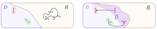
Given a graph $G$ and an associated ${Z^{2}}$ from zipper constraint collection ${\color[rgb]{0,0.25,0.25}\mathcal{Z}}$ , let ${\color[rgb]{0.0,0.0,0.4}R}\subseteq{Z^{2}}$ be a set of pairs such that for every pair $\{{u},{w}\}$ in ${\color[rgb]{0.0,0.0,0.4}R}$ , $u$ and $w$ have comparable neighborhoods. If ${\color[rgb]{0.0,0.0,0.4}\underline{R}}\subseteq{\color[rgb]{0.0,0.0,0.4}R}$ then let $\mathscr{S}_{{\color[rgb]{0.0,0.0,0.4}\underline{R}}}\coloneqq\{({U_{i}};{W_{i}})\in Z_{\mathscr{F}}\;|\;U_{i}\in{\color[rgb]{0.0,0.0,0.4}\underline{R}}\}$ and $\mathscr{D}_{{\color[rgb]{0.0,0.0,0.4}\underline{R}}}\coloneqq\{({U_{j}};{W_{j}})\in Z_{\mathscr{F}}\;|\;W_{j}\in{\color[rgb]{0.0,0.0,0.4}\underline{R}}\}$ . If $\mathbb{K}$ is a cover for $G$ , then there is a cover $\widetilde{\mathbb{K}}$ , no larger than $\mathbb{K}$ , such that:

1.

$\widetilde{\mathbb{K}}$ is a clique cover of $G$ that satisfies the specific zipper constraints $\mathscr{S}_{{\color[rgb]{0.0,0.0,0.4}\underline{R}}}\cap\mathscr{D}_{{\color[rgb]{0.0,0.0,0.4}\underline{R}}}$ .
2.

If $\mathbb{K}$ satisfies the zipper constraints $C\subseteq{\color[rgb]{0,0.25,0.25}\mathcal{Z}}$ , and $\widetilde{\mathbb{K}}$ satisfies the zipper constraints $\widetilde{C}\subseteq{\color[rgb]{0,0.25,0.25}\mathcal{Z}}$ , and then ${C}\setminus\widetilde{C}\subseteq\mathscr{S}_{{\color[rgb]{0.0,0.0,0.4}\underline{R}}}\setminus\mathscr{D}_{{\color[rgb]{0.0,0.0,0.4}\underline{R}}}$ .

The intuition is that we can repair $\mathbb{K}$ , without increasing its size, to ensure that those zipper constraints wholly in ${\color[rgb]{0.0,0.0,0.4}\underline{R}}$ will hold (item 1). This process can have an unfortunate side-effect of breaking some zipper constraints which held formerly: but those are only the zipper constraints that ‘depart’ ${\color[rgb]{0.0,0.0,0.4}\underline{R}}$ , i.e., $\mathscr{S}_{{\color[rgb]{0.0,0.0,0.4}\underline{R}}}\setminus\mathscr{D}_{{\color[rgb]{0.0,0.0,0.4}\underline{R}}}$ (item 2).

Proof.

Let $\mathbb{K}=\{K_{1},K_{2},\dots,K_{m}\}$ . Collect all the interior pairs $\mathcal{I}\coloneqq\{W_{i}\in Z_{\scalebox{0.5}{\text{tgt}}}^{2}\;|\;({U_{i}};{W_{i}})\in\mathscr{S}_{{\color[rgb]{0.0,0.0,0.4}\underline{R}}}\cap\mathscr{D}_{{\color[rgb]{0.0,0.0,0.4}\underline{R}}}\}$ . Starting with cover $\mathbb{K}^{({0})}=\mathbb{K}$ , we iterate over collection $\mathcal{I}$ and modify the cover incrementally. Form $\mathbb{K}^{({i})}$ from $\mathbb{K}^{({i-1})}$ by taking the $i^{\rm th}$ pair $\{{u},{w}\}$ from $\mathcal{I}$ and doing the following: if $\mathcal{N}_{G}(u)\subseteq\mathcal{N}_{G}(w)$ then, first, copy those $K_{\ell}\in\mathbb{K}^{({i-1})}$ not containing $u$ to $\mathbb{K}^{({i})}$ ; next, gather those $K_{j}\in\mathbb{K}^{({i-1})}$ containing $u$ and place $K_{j}\cup\{w\}$ in $\mathbb{K}^{({i})}$ . Otherwise, $\mathcal{N}_{G}(u)\supseteq\mathcal{N}_{G}(w)$ , so do the same two operations but reverse the roles of $v$ and $w$ . Once this iteration has been completed, take $\widetilde{\mathbb{K}}=\mathbb{K}^{({|\mathcal{I}|})}$ .

In the construction above, ‘coverness’ must be preserved as the sets in $\mathbb{K}^{({i})}$ only grow with each subsequent $i$ . Because, when $w$ is added to a clique containing $v$ , the former must already be compatible with all those vertices in the clique —via the comparable neighborhoods property— the set $K_{j}\cup\{w\}$ is a clique too. Also, every zipper constraint in $\mathscr{S}_{{\color[rgb]{0.0,0.0,0.4}\underline{R}}}\cap\mathscr{D}_{{\color[rgb]{0.0,0.0,0.4}\underline{R}}}$ is satisfied because every destination pair of each such zipper constraint will appear in some clique in $\widetilde{\mathbb{K}}$ . Further, $|\widetilde{\mathbb{K}}|\leq m$ .

For the second property, notice that in $\widetilde{\mathbb{K}}$ the only pairs that have changed are those in $\mathcal{I}$ ; they have been altered by including some vertices in a common clique, where before they had been separated. But this change can only alter the satisfaction of constraints for which those pairs act as sources, viz. $\mathscr{S}_{{\color[rgb]{0.0,0.0,0.4}\underline{R}}}$ . So ${C}\setminus\widetilde{C}\subseteq\mathscr{S}_{{\color[rgb]{0.0,0.0,0.4}\underline{R}}}$ . But, as just established, those elements in $\mathscr{S}_{{\color[rgb]{0.0,0.0,0.4}\underline{R}}}\cap\mathscr{D}_{{\color[rgb]{0.0,0.0,0.4}\underline{R}}}$ are satisfied, so ${C}\setminus\widetilde{C}$ cannot include pairs in $\mathscr{D}_{{\color[rgb]{0.0,0.0,0.4}\underline{R}}}$ , thus the claim follows. ∎

The preceding shows that zipper constraints with both ends in a set ${\color[rgb]{0.0,0.0,0.4}\underline{R}}\subseteq{\color[rgb]{0.0,0.0,0.4}R}$ which possesses comparable neighborhoods, need not cause any trouble. Our prior discussion, using downstream-enabled prescriptions, allows one to deal with constraints entirely outside of ${\color[rgb]{0.0,0.0,0.4}R}$ . However, a remaining difficulty is that some constraints may straddle the two sets. We put ${\color[rgb]{0.0,0.0,0.4}R}$ aside briefly, returning to it again in Lemma 22 and subsequent theorems, as we now introduce extra machinery for the liminal constraints.

Broadly speaking, the preceding shows that rather than taking ${\color[rgb]{0.0,0.0,0.4}D}={Z^{2}}$ we can avoid having to include the comparable-neighborhood pairs in the enumeration. This idea is close to being correct, but we need to ensure ${\color[rgb]{0.0,0.0,0.4}D}$ will handle the liminal constraints correctly as well. To do this, the idea will be to expand the domain ${\color[rgb]{0.0,0.0,0.4}D}$ to embrace some additional pairs. (The additional pairs are those, when interpreted back in the filter, whose merger or non-merger is entailed from the choices made in a given prescription on ${\color[rgb]{0.0,0.0,0.4}D}$ .)

Construction 20 (Prescription Boundary Inclusion).

Given a prescription $\mathbb{S}^{\scalebox{0.5}{\text{ON}}}_{{\color[rgb]{0.0,0.0,0.4}D}}$ , we modify it by increasing $\mathbb{S}^{\scalebox{0.5}{\text{ON}}}_{{\color[rgb]{0.0,0.0,0.4}D}}$ and $\mathbb{S}^{\scalebox{0.5}{\text{OFF}}}_{{\color[rgb]{0.0,0.0,0.4}D}}$ . This is achieved, firstly, by modifying its domain and then, secondly, by selecting some additional elements, which transforms it into a new prescription. To do so, define sets:

1.

Upstream vertex pairs of the off pairs should be treated as if they were turned off too, i.e., prohibited from being in a clique together (the constraint cannot be satisfied otherwise); let $\mathcal{F}^{\textsc{off}}_{\color[rgb]{0.0,0.0,0.4}D}(\mathbb{S}^{\scalebox{0.5}{\text{ON}}}_{{\color[rgb]{0.0,0.0,0.4}D}})=\{P_{a}\in{Z^{2}}\setminus{\color[rgb]{0.0,0.0,0.4}D}\;|\;\exists P_{b}\in{\color[rgb]{0.0,0.0,0.4}D}\setminus\mathbb{S}^{\scalebox{0.5}{\text{ON}}}_{{\color[rgb]{0.0,0.0,0.4}D}},P_{a}\mathrlap{\raisebox{1.0pt}{${}^{\,\ast}$}}{\,\prec\,}P_{b}\}$ .
2.

Downstream vertex pairs of the on pairs should be turned on as well, i.e. must be in some clique together; let $\mathcal{F}^{\textsc{on}}_{\color[rgb]{0.0,0.0,0.4}D}(\mathbb{S}^{\scalebox{0.5}{\text{ON}}}_{{\color[rgb]{0.0,0.0,0.4}D}})=\{P_{c}\in{Z^{2}}\setminus{\color[rgb]{0.0,0.0,0.4}D}\;|\;\exists P_{d}\in\mathbb{S}^{\scalebox{0.5}{\text{ON}}}_{{\color[rgb]{0.0,0.0,0.4}D}},P_{d}\mathrlap{\raisebox{1.0pt}{${}^{\,\ast}$}}{\,\prec\,}P_{c}\}$ .

Construct a derived prescription by expanding the domain and on pairs as

\mathchoice{\hbox to0.0pt{\hbox to8.55695pt{\hfill{\color[rgb]{0.0,0.0,0.4}$\overline{\vrule width=0.0pt,height=6.83331pt\kern 6.50694pt}$}}\hss}\hbox{\set@color$\displaystyle{\color[rgb]{0.0,0.0,0.4}D}$}}{\hbox to0.0pt{\hbox to8.55695pt{\hfill{\color[rgb]{0.0,0.0,0.4}$\overline{\vrule width=0.0pt,height=6.83331pt\kern 6.50694pt}$}}\hss}\hbox{\set@color$\textstyle{\color[rgb]{0.0,0.0,0.4}D}$}}{\hbox to0.0pt{\hbox to5.98985pt{\hfill{\color[rgb]{0.0,0.0,0.4}$\overline{\vrule width=0.0pt,height=4.78333pt\kern 4.55486pt}$}}\hss}\hbox{\set@color$\scriptstyle{\color[rgb]{0.0,0.0,0.4}D}$}}{\hbox to0.0pt{\hbox to4.27846pt{\hfill{\color[rgb]{0.0,0.0,0.4}$\overline{\vrule width=0.0pt,height=3.41666pt\kern 3.25346pt}$}}\hss}\hbox{\set@color$\scriptscriptstyle{\color[rgb]{0.0,0.0,0.4}D}$}}\coloneqq{\color[rgb]{0.0,0.0,0.4}D}\cup\mathcal{F}^{\textsc{off}}_{\color[rgb]{0.0,0.0,0.4}D}(\mathbb{S}^{\scalebox{0.5}{\text{ON}}}_{{\color[rgb]{0.0,0.0,0.4}D}})\cup\mathcal{F}^{\textsc{on}}_{\color[rgb]{0.0,0.0,0.4}D}(\mathbb{S}^{\scalebox{0.5}{\text{ON}}}_{{\color[rgb]{0.0,0.0,0.4}D}}),\text{ and }\mathbb{S}^{\scalebox{0.5}{\text{ON}}}_{\mathchoice{\hbox to0.0pt{\hbox to5.98985pt{\hfill{\color[rgb]{0.0,0.0,0.4}$\overline{\vrule width=0.0pt,height=4.78333pt\kern 4.55486pt}$}}\hss}\hbox{\set@color$\displaystyle{\color[rgb]{0.0,0.0,0.4}D}$}}{\hbox to0.0pt{\hbox to5.98985pt{\hfill{\color[rgb]{0.0,0.0,0.4}$\overline{\vrule width=0.0pt,height=4.78333pt\kern 4.55486pt}$}}\hss}\hbox{\set@color$\textstyle{\color[rgb]{0.0,0.0,0.4}D}$}}{\hbox to0.0pt{\hbox to4.1929pt{\hfill{\color[rgb]{0.0,0.0,0.4}$\overline{\vrule width=0.0pt,height=3.34833pt\kern 3.1884pt}$}}\hss}\hbox{\set@color$\scriptstyle{\color[rgb]{0.0,0.0,0.4}D}$}}{\hbox to0.0pt{\hbox to2.99492pt{\hfill{\color[rgb]{0.0,0.0,0.4}$\overline{\vrule width=0.0pt,height=2.39166pt\kern 2.27742pt}$}}\hss}\hbox{\set@color$\scriptscriptstyle{\color[rgb]{0.0,0.0,0.4}D}$}}}\coloneqq\mathbb{S}^{\scalebox{0.5}{\text{ON}}}_{{\color[rgb]{0.0,0.0,0.4}D}}\cup\mathcal{F}^{\textsc{on}}_{\color[rgb]{0.0,0.0,0.4}D}(\mathbb{S}^{\scalebox{0.5}{\text{ON}}}_{{\color[rgb]{0.0,0.0,0.4}D}}),

where the on pairs have grown to include those in $\mathcal{F}^{\textsc{on}}_{\color[rgb]{0.0,0.0,0.4}D}$ . And, as before, the off pairs are those in $\mathchoice{\hbox to0.0pt{\hbox to8.55695pt{\hfill{\color[rgb]{0.0,0.0,0.4}$\overline{\vrule width=0.0pt,height=6.83331pt\kern 6.50694pt}$}}\hss}\hbox{\set@color$\displaystyle{\color[rgb]{0.0,0.0,0.4}D}$}}{\hbox to0.0pt{\hbox to8.55695pt{\hfill{\color[rgb]{0.0,0.0,0.4}$\overline{\vrule width=0.0pt,height=6.83331pt\kern 6.50694pt}$}}\hss}\hbox{\set@color$\textstyle{\color[rgb]{0.0,0.0,0.4}D}$}}{\hbox to0.0pt{\hbox to5.98985pt{\hfill{\color[rgb]{0.0,0.0,0.4}$\overline{\vrule width=0.0pt,height=4.78333pt\kern 4.55486pt}$}}\hss}\hbox{\set@color$\scriptstyle{\color[rgb]{0.0,0.0,0.4}D}$}}{\hbox to0.0pt{\hbox to4.27846pt{\hfill{\color[rgb]{0.0,0.0,0.4}$\overline{\vrule width=0.0pt,height=3.41666pt\kern 3.25346pt}$}}\hss}\hbox{\set@color$\scriptscriptstyle{\color[rgb]{0.0,0.0,0.4}D}$}}\setminus\mathbb{S}^{\scalebox{0.5}{\text{ON}}}_{\mathchoice{\hbox to0.0pt{\hbox to5.98985pt{\hfill{\color[rgb]{0.0,0.0,0.4}$\overline{\vrule width=0.0pt,height=4.78333pt\kern 4.55486pt}$}}\hss}\hbox{\set@color$\displaystyle{\color[rgb]{0.0,0.0,0.4}D}$}}{\hbox to0.0pt{\hbox to5.98985pt{\hfill{\color[rgb]{0.0,0.0,0.4}$\overline{\vrule width=0.0pt,height=4.78333pt\kern 4.55486pt}$}}\hss}\hbox{\set@color$\textstyle{\color[rgb]{0.0,0.0,0.4}D}$}}{\hbox to0.0pt{\hbox to4.1929pt{\hfill{\color[rgb]{0.0,0.0,0.4}$\overline{\vrule width=0.0pt,height=3.34833pt\kern 3.1884pt}$}}\hss}\hbox{\set@color$\scriptstyle{\color[rgb]{0.0,0.0,0.4}D}$}}{\hbox to0.0pt{\hbox to2.99492pt{\hfill{\color[rgb]{0.0,0.0,0.4}$\overline{\vrule width=0.0pt,height=2.39166pt\kern 2.27742pt}$}}\hss}\hbox{\set@color$\scriptscriptstyle{\color[rgb]{0.0,0.0,0.4}D}$}}}$ ; and the prescription is silent about the elements outside $\overline{\vrule width=0.0pt,height=6.83331pt\kern 6.50694pt}$ $\textstyle{\color[rgb]{0.0,0.0,0.4}D}$ .

Caution: in $\mathbb{S}^{\scalebox{0.5}{\text{ON}}}_{\mathchoice{\hbox to0.0pt{\hbox to5.98985pt{\hfill{\color[rgb]{0.0,0.0,0.4}$\overline{\vrule width=0.0pt,height=4.78333pt\kern 4.55486pt}$}}\hss}\hbox{\set@color$\displaystyle{\color[rgb]{0.0,0.0,0.4}D}$}}{\hbox to0.0pt{\hbox to5.98985pt{\hfill{\color[rgb]{0.0,0.0,0.4}$\overline{\vrule width=0.0pt,height=4.78333pt\kern 4.55486pt}$}}\hss}\hbox{\set@color$\textstyle{\color[rgb]{0.0,0.0,0.4}D}$}}{\hbox to0.0pt{\hbox to4.1929pt{\hfill{\color[rgb]{0.0,0.0,0.4}$\overline{\vrule width=0.0pt,height=3.34833pt\kern 3.1884pt}$}}\hss}\hbox{\set@color$\scriptstyle{\color[rgb]{0.0,0.0,0.4}D}$}}{\hbox to0.0pt{\hbox to2.99492pt{\hfill{\color[rgb]{0.0,0.0,0.4}$\overline{\vrule width=0.0pt,height=2.39166pt\kern 2.27742pt}$}}\hss}\hbox{\set@color$\scriptscriptstyle{\color[rgb]{0.0,0.0,0.4}D}$}}}$ we have lightened the notation by eliding the dependence of $\overline{\vrule width=0.0pt,height=6.83331pt\kern 6.50694pt}$ $\textstyle{\color[rgb]{0.0,0.0,0.4}D}$ on $\mathbb{S}^{\scalebox{0.5}{\text{ON}}}_{{\color[rgb]{0.0,0.0,0.4}D}}$ . Care is warranted because $\overline{\vrule width=0.0pt,height=6.83331pt\kern 6.50694pt}$ $\textstyle{\color[rgb]{0.0,0.0,0.4}D}$ cannot be constructed from ${\color[rgb]{0.0,0.0,0.4}D}$ alone—different prescriptions will give different $\overline{\vrule width=0.0pt,height=6.83331pt\kern 6.50694pt}$ $\textstyle{\color[rgb]{0.0,0.0,0.4}D}$ s.

Property 21.

If prescription $\mathbb{S}^{\scalebox{0.5}{\text{ON}}}_{{\color[rgb]{0.0,0.0,0.4}D}}$ is downstream enabled then $\mathbb{S}^{\scalebox{0.5}{\text{ON}}}_{\mathchoice{\hbox to0.0pt{\hbox to5.98985pt{\hfill{\color[rgb]{0.0,0.0,0.4}$\overline{\vrule width=0.0pt,height=4.78333pt\kern 4.55486pt}$}}\hss}\hbox{\set@color$\displaystyle{\color[rgb]{0.0,0.0,0.4}D}$}}{\hbox to0.0pt{\hbox to5.98985pt{\hfill{\color[rgb]{0.0,0.0,0.4}$\overline{\vrule width=0.0pt,height=4.78333pt\kern 4.55486pt}$}}\hss}\hbox{\set@color$\textstyle{\color[rgb]{0.0,0.0,0.4}D}$}}{\hbox to0.0pt{\hbox to4.1929pt{\hfill{\color[rgb]{0.0,0.0,0.4}$\overline{\vrule width=0.0pt,height=3.34833pt\kern 3.1884pt}$}}\hss}\hbox{\set@color$\scriptstyle{\color[rgb]{0.0,0.0,0.4}D}$}}{\hbox to0.0pt{\hbox to2.99492pt{\hfill{\color[rgb]{0.0,0.0,0.4}$\overline{\vrule width=0.0pt,height=2.39166pt\kern 2.27742pt}$}}\hss}\hbox{\set@color$\scriptscriptstyle{\color[rgb]{0.0,0.0,0.4}D}$}}}$ is downstream enabled.

Proof.

We prove a slightly stronger statement, which is that $(P_{a}\in\mathbb{S}^{\scalebox{0.5}{\text{ON}}}_{\mathchoice{\hbox to0.0pt{\hbox to5.98985pt{\hfill{\color[rgb]{0.0,0.0,0.4}$\overline{\vrule width=0.0pt,height=4.78333pt\kern 4.55486pt}$}}\hss}\hbox{\set@color$\displaystyle{\color[rgb]{0.0,0.0,0.4}D}$}}{\hbox to0.0pt{\hbox to5.98985pt{\hfill{\color[rgb]{0.0,0.0,0.4}$\overline{\vrule width=0.0pt,height=4.78333pt\kern 4.55486pt}$}}\hss}\hbox{\set@color$\textstyle{\color[rgb]{0.0,0.0,0.4}D}$}}{\hbox to0.0pt{\hbox to4.1929pt{\hfill{\color[rgb]{0.0,0.0,0.4}$\overline{\vrule width=0.0pt,height=3.34833pt\kern 3.1884pt}$}}\hss}\hbox{\set@color$\scriptstyle{\color[rgb]{0.0,0.0,0.4}D}$}}{\hbox to0.0pt{\hbox to2.99492pt{\hfill{\color[rgb]{0.0,0.0,0.4}$\overline{\vrule width=0.0pt,height=2.39166pt\kern 2.27742pt}$}}\hss}\hbox{\set@color$\scriptscriptstyle{\color[rgb]{0.0,0.0,0.4}D}$}}})\wedge(P_{a}\mathrlap{\raisebox{1.0pt}{${}^{\,\ast}$}}{\,\prec\,}P_{b})\implies(P_{b}\in\mathbb{S}^{\scalebox{0.5}{\text{ON}}}_{\mathchoice{\hbox to0.0pt{\hbox to5.98985pt{\hfill{\color[rgb]{0.0,0.0,0.4}$\overline{\vrule width=0.0pt,height=4.78333pt\kern 4.55486pt}$}}\hss}\hbox{\set@color$\displaystyle{\color[rgb]{0.0,0.0,0.4}D}$}}{\hbox to0.0pt{\hbox to5.98985pt{\hfill{\color[rgb]{0.0,0.0,0.4}$\overline{\vrule width=0.0pt,height=4.78333pt\kern 4.55486pt}$}}\hss}\hbox{\set@color$\textstyle{\color[rgb]{0.0,0.0,0.4}D}$}}{\hbox to0.0pt{\hbox to4.1929pt{\hfill{\color[rgb]{0.0,0.0,0.4}$\overline{\vrule width=0.0pt,height=3.34833pt\kern 3.1884pt}$}}\hss}\hbox{\set@color$\scriptstyle{\color[rgb]{0.0,0.0,0.4}D}$}}{\hbox to0.0pt{\hbox to2.99492pt{\hfill{\color[rgb]{0.0,0.0,0.4}$\overline{\vrule width=0.0pt,height=2.39166pt\kern 2.27742pt}$}}\hss}\hbox{\set@color$\scriptscriptstyle{\color[rgb]{0.0,0.0,0.4}D}$}}})$ . Given that antecedent, we have $P_{a}\in\mathbb{S}^{\scalebox{0.5}{\text{ON}}}_{{\color[rgb]{0.0,0.0,0.4}D}}$ or $P_{a}\in\mathcal{F}^{\textsc{on}}_{\color[rgb]{0.0,0.0,0.4}D}(\mathbb{S}^{\scalebox{0.5}{\text{ON}}}_{{\color[rgb]{0.0,0.0,0.4}D}})$ , since $\mathbb{S}^{\scalebox{0.5}{\text{ON}}}_{\mathchoice{\hbox to0.0pt{\hbox to5.98985pt{\hfill{\color[rgb]{0.0,0.0,0.4}$\overline{\vrule width=0.0pt,height=4.78333pt\kern 4.55486pt}$}}\hss}\hbox{\set@color$\displaystyle{\color[rgb]{0.0,0.0,0.4}D}$}}{\hbox to0.0pt{\hbox to5.98985pt{\hfill{\color[rgb]{0.0,0.0,0.4}$\overline{\vrule width=0.0pt,height=4.78333pt\kern 4.55486pt}$}}\hss}\hbox{\set@color$\textstyle{\color[rgb]{0.0,0.0,0.4}D}$}}{\hbox to0.0pt{\hbox to4.1929pt{\hfill{\color[rgb]{0.0,0.0,0.4}$\overline{\vrule width=0.0pt,height=3.34833pt\kern 3.1884pt}$}}\hss}\hbox{\set@color$\scriptstyle{\color[rgb]{0.0,0.0,0.4}D}$}}{\hbox to0.0pt{\hbox to2.99492pt{\hfill{\color[rgb]{0.0,0.0,0.4}$\overline{\vrule width=0.0pt,height=2.39166pt\kern 2.27742pt}$}}\hss}\hbox{\set@color$\scriptscriptstyle{\color[rgb]{0.0,0.0,0.4}D}$}}}=\mathbb{S}^{\scalebox{0.5}{\text{ON}}}_{{\color[rgb]{0.0,0.0,0.4}D}}\cup\mathcal{F}^{\textsc{on}}_{\color[rgb]{0.0,0.0,0.4}D}(\mathbb{S}^{\scalebox{0.5}{\text{ON}}}_{{\color[rgb]{0.0,0.0,0.4}D}})$ . Then we need to show

1.

$(P_{a}\in\mathbb{S}^{\scalebox{0.5}{\text{ON}}}_{{\color[rgb]{0.0,0.0,0.4}D}})\wedge(P_{a}\mathrlap{\raisebox{1.0pt}{${}^{\,\ast}$}}{\,\prec\,}P_{b})\implies(P_{b}\in\mathbb{S}^{\scalebox{0.5}{\text{ON}}}_{\mathchoice{\hbox to0.0pt{\hbox to5.98985pt{\hfill{\color[rgb]{0.0,0.0,0.4}$\overline{\vrule width=0.0pt,height=4.78333pt\kern 4.55486pt}$}}\hss}\hbox{\set@color$\displaystyle{\color[rgb]{0.0,0.0,0.4}D}$}}{\hbox to0.0pt{\hbox to5.98985pt{\hfill{\color[rgb]{0.0,0.0,0.4}$\overline{\vrule width=0.0pt,height=4.78333pt\kern 4.55486pt}$}}\hss}\hbox{\set@color$\textstyle{\color[rgb]{0.0,0.0,0.4}D}$}}{\hbox to0.0pt{\hbox to4.1929pt{\hfill{\color[rgb]{0.0,0.0,0.4}$\overline{\vrule width=0.0pt,height=3.34833pt\kern 3.1884pt}$}}\hss}\hbox{\set@color$\scriptstyle{\color[rgb]{0.0,0.0,0.4}D}$}}{\hbox to0.0pt{\hbox to2.99492pt{\hfill{\color[rgb]{0.0,0.0,0.4}$\overline{\vrule width=0.0pt,height=2.39166pt\kern 2.27742pt}$}}\hss}\hbox{\set@color$\scriptscriptstyle{\color[rgb]{0.0,0.0,0.4}D}$}}})$ and
2.

$(P_{a}\in\mathcal{F}^{\textsc{on}}_{\color[rgb]{0.0,0.0,0.4}D}(\mathbb{S}^{\scalebox{0.5}{\text{ON}}}_{{\color[rgb]{0.0,0.0,0.4}D}}))\wedge(P_{a}\mathrlap{\raisebox{1.0pt}{${}^{\,\ast}$}}{\,\prec\,}P_{b})\implies(P_{b}\in\mathbb{S}^{\scalebox{0.5}{\text{ON}}}_{\mathchoice{\hbox to0.0pt{\hbox to5.98985pt{\hfill{\color[rgb]{0.0,0.0,0.4}$\overline{\vrule width=0.0pt,height=4.78333pt\kern 4.55486pt}$}}\hss}\hbox{\set@color$\displaystyle{\color[rgb]{0.0,0.0,0.4}D}$}}{\hbox to0.0pt{\hbox to5.98985pt{\hfill{\color[rgb]{0.0,0.0,0.4}$\overline{\vrule width=0.0pt,height=4.78333pt\kern 4.55486pt}$}}\hss}\hbox{\set@color$\textstyle{\color[rgb]{0.0,0.0,0.4}D}$}}{\hbox to0.0pt{\hbox to4.1929pt{\hfill{\color[rgb]{0.0,0.0,0.4}$\overline{\vrule width=0.0pt,height=3.34833pt\kern 3.1884pt}$}}\hss}\hbox{\set@color$\scriptstyle{\color[rgb]{0.0,0.0,0.4}D}$}}{\hbox to0.0pt{\hbox to2.99492pt{\hfill{\color[rgb]{0.0,0.0,0.4}$\overline{\vrule width=0.0pt,height=2.39166pt\kern 2.27742pt}$}}\hss}\hbox{\set@color$\scriptscriptstyle{\color[rgb]{0.0,0.0,0.4}D}$}}})$ .

For the first, $P_{b}$ is certainly in $\mathbb{S}^{\scalebox{0.5}{\text{ON}}}_{\mathchoice{\hbox to0.0pt{\hbox to5.98985pt{\hfill{\color[rgb]{0.0,0.0,0.4}$\overline{\vrule width=0.0pt,height=4.78333pt\kern 4.55486pt}$}}\hss}\hbox{\set@color$\displaystyle{\color[rgb]{0.0,0.0,0.4}D}$}}{\hbox to0.0pt{\hbox to5.98985pt{\hfill{\color[rgb]{0.0,0.0,0.4}$\overline{\vrule width=0.0pt,height=4.78333pt\kern 4.55486pt}$}}\hss}\hbox{\set@color$\textstyle{\color[rgb]{0.0,0.0,0.4}D}$}}{\hbox to0.0pt{\hbox to4.1929pt{\hfill{\color[rgb]{0.0,0.0,0.4}$\overline{\vrule width=0.0pt,height=3.34833pt\kern 3.1884pt}$}}\hss}\hbox{\set@color$\scriptstyle{\color[rgb]{0.0,0.0,0.4}D}$}}{\hbox to0.0pt{\hbox to2.99492pt{\hfill{\color[rgb]{0.0,0.0,0.4}$\overline{\vrule width=0.0pt,height=2.39166pt\kern 2.27742pt}$}}\hss}\hbox{\set@color$\scriptscriptstyle{\color[rgb]{0.0,0.0,0.4}D}$}}}$ : When $P_{b}\not\in{\color[rgb]{0.0,0.0,0.4}D}$ then Construction 20 ensures $P_{b}\in\mathcal{F}^{\textsc{on}}_{\color[rgb]{0.0,0.0,0.4}D}(\mathbb{S}^{\scalebox{0.5}{\text{ON}}}_{{\color[rgb]{0.0,0.0,0.4}D}})$ ; alternatively, when $P_{b}\in{\color[rgb]{0.0,0.0,0.4}D}$ then $P_{b}\in\mathbb{S}^{\scalebox{0.5}{\text{ON}}}_{{\color[rgb]{0.0,0.0,0.4}D}}\subseteq\mathbb{S}^{\scalebox{0.5}{\text{ON}}}_{\mathchoice{\hbox to0.0pt{\hbox to5.98985pt{\hfill{\color[rgb]{0.0,0.0,0.4}$\overline{\vrule width=0.0pt,height=4.78333pt\kern 4.55486pt}$}}\hss}\hbox{\set@color$\displaystyle{\color[rgb]{0.0,0.0,0.4}D}$}}{\hbox to0.0pt{\hbox to5.98985pt{\hfill{\color[rgb]{0.0,0.0,0.4}$\overline{\vrule width=0.0pt,height=4.78333pt\kern 4.55486pt}$}}\hss}\hbox{\set@color$\textstyle{\color[rgb]{0.0,0.0,0.4}D}$}}{\hbox to0.0pt{\hbox to4.1929pt{\hfill{\color[rgb]{0.0,0.0,0.4}$\overline{\vrule width=0.0pt,height=3.34833pt\kern 3.1884pt}$}}\hss}\hbox{\set@color$\scriptstyle{\color[rgb]{0.0,0.0,0.4}D}$}}{\hbox to0.0pt{\hbox to2.99492pt{\hfill{\color[rgb]{0.0,0.0,0.4}$\overline{\vrule width=0.0pt,height=2.39166pt\kern 2.27742pt}$}}\hss}\hbox{\set@color$\scriptscriptstyle{\color[rgb]{0.0,0.0,0.4}D}$}}}$ due to the original prescription being downstream enabled.

For the second, the definition of $\mathcal{F}^{\textsc{on}}_{\color[rgb]{0.0,0.0,0.4}D}(\mathbb{S}^{\scalebox{0.5}{\text{ON}}}_{{\color[rgb]{0.0,0.0,0.4}D}})$ means there is some pair $P_{d}\mathrlap{\raisebox{1.0pt}{${}^{\,\ast}$}}{\,\prec\,}P_{a}$ with $P_{d}\in\mathbb{S}^{\scalebox{0.5}{\text{ON}}}_{{\color[rgb]{0.0,0.0,0.4}D}}$ . Transitivity and $P_{a}\mathrlap{\raisebox{1.0pt}{${}^{\,\ast}$}}{\,\prec\,}P_{b}$ means $P_{d}\mathrlap{\raisebox{1.0pt}{${}^{\,\ast}$}}{\,\prec\,}P_{b}$ . Again, $P_{b}$ is certainly in $\mathbb{S}^{\scalebox{0.5}{\text{ON}}}_{\mathchoice{\hbox to0.0pt{\hbox to5.98985pt{\hfill{\color[rgb]{0.0,0.0,0.4}$\overline{\vrule width=0.0pt,height=4.78333pt\kern 4.55486pt}$}}\hss}\hbox{\set@color$\displaystyle{\color[rgb]{0.0,0.0,0.4}D}$}}{\hbox to0.0pt{\hbox to5.98985pt{\hfill{\color[rgb]{0.0,0.0,0.4}$\overline{\vrule width=0.0pt,height=4.78333pt\kern 4.55486pt}$}}\hss}\hbox{\set@color$\textstyle{\color[rgb]{0.0,0.0,0.4}D}$}}{\hbox to0.0pt{\hbox to4.1929pt{\hfill{\color[rgb]{0.0,0.0,0.4}$\overline{\vrule width=0.0pt,height=3.34833pt\kern 3.1884pt}$}}\hss}\hbox{\set@color$\scriptstyle{\color[rgb]{0.0,0.0,0.4}D}$}}{\hbox to0.0pt{\hbox to2.99492pt{\hfill{\color[rgb]{0.0,0.0,0.4}$\overline{\vrule width=0.0pt,height=2.39166pt\kern 2.27742pt}$}}\hss}\hbox{\set@color$\scriptscriptstyle{\color[rgb]{0.0,0.0,0.4}D}$}}}$ , using the argument above but with $P_{d}$ fulfilling the role of $P_{a}$ before. ∎

(Note, as per the discussion at the end of Section 5, when ${\color[rgb]{0.0,0.0,0.4}D}={Z^{2}}$ , then $\mathchoice{\hbox to0.0pt{\hbox to8.55695pt{\hfill{\color[rgb]{0.0,0.0,0.4}$\overline{\vrule width=0.0pt,height=6.83331pt\kern 6.50694pt}$}}\hss}\hbox{\set@color$\displaystyle{\color[rgb]{0.0,0.0,0.4}D}$}}{\hbox to0.0pt{\hbox to8.55695pt{\hfill{\color[rgb]{0.0,0.0,0.4}$\overline{\vrule width=0.0pt,height=6.83331pt\kern 6.50694pt}$}}\hss}\hbox{\set@color$\textstyle{\color[rgb]{0.0,0.0,0.4}D}$}}{\hbox to0.0pt{\hbox to5.98985pt{\hfill{\color[rgb]{0.0,0.0,0.4}$\overline{\vrule width=0.0pt,height=4.78333pt\kern 4.55486pt}$}}\hss}\hbox{\set@color$\scriptstyle{\color[rgb]{0.0,0.0,0.4}D}$}}{\hbox to0.0pt{\hbox to4.27846pt{\hfill{\color[rgb]{0.0,0.0,0.4}$\overline{\vrule width=0.0pt,height=3.41666pt\kern 3.25346pt}$}}\hss}\hbox{\set@color$\scriptscriptstyle{\color[rgb]{0.0,0.0,0.4}D}$}}={\color[rgb]{0.0,0.0,0.4}D}={Z^{2}}$ , and we have $\mathbb{S}^{\scalebox{0.5}{\text{ON}}}_{\mathchoice{\hbox to0.0pt{\hbox to5.98985pt{\hfill{\color[rgb]{0.0,0.0,0.4}$\overline{\vrule width=0.0pt,height=4.78333pt\kern 4.55486pt}$}}\hss}\hbox{\set@color$\displaystyle{\color[rgb]{0.0,0.0,0.4}D}$}}{\hbox to0.0pt{\hbox to5.98985pt{\hfill{\color[rgb]{0.0,0.0,0.4}$\overline{\vrule width=0.0pt,height=4.78333pt\kern 4.55486pt}$}}\hss}\hbox{\set@color$\textstyle{\color[rgb]{0.0,0.0,0.4}D}$}}{\hbox to0.0pt{\hbox to4.1929pt{\hfill{\color[rgb]{0.0,0.0,0.4}$\overline{\vrule width=0.0pt,height=3.34833pt\kern 3.1884pt}$}}\hss}\hbox{\set@color$\scriptstyle{\color[rgb]{0.0,0.0,0.4}D}$}}{\hbox to0.0pt{\hbox to2.99492pt{\hfill{\color[rgb]{0.0,0.0,0.4}$\overline{\vrule width=0.0pt,height=2.39166pt\kern 2.27742pt}$}}\hss}\hbox{\set@color$\scriptscriptstyle{\color[rgb]{0.0,0.0,0.4}D}$}}}=\mathbb{S}^{\scalebox{0.5}{\text{ON}}}_{{\color[rgb]{0.0,0.0,0.4}D}}=\mathbb{S}^{\scalebox{0.5}{\text{ON}}}_{{Z^{2}}}$ so long as $\mathbb{S}^{\scalebox{0.5}{\text{ON}}}_{{\color[rgb]{0.0,0.0,0.4}D}}$ was downstream enabled.)

7 Main result: FPT algorithm

The paper’s key algorithm just assembles all the pieces presented up to this point; it appears in Algorithm 2. The following lemma and theorem provide its correctness, while the final corollary gives the parameterized running-time.

Algorithm 2 Solve

MZCC

({G},{{\color[rgb]{0,0.25,0.25}\mathcal{Z}}})

0: Compatibility graph

G

, zipper constraints

\mathcal{Z}

0: Clique cover

\mathbb{K}_{\text{best}}

with minimum cardinality

1: Take

{\color[rgb]{0.0,0.0,0.4}D}={Z^{2}}\setminus{\color[rgb]{0.0,0.0,0.4}R}

2: Initialize

\mathbb{K}_{\text{best}}\leftarrow\big{\{}\{v\}\mid v\in V(G)\big{\}}

3: for

\mathbb{S}^{\scalebox{0.5}{\text{ON}}}_{{\color[rgb]{0.0,0.0,0.4}D}}\in{\color[rgb]{0.375,0,0.125}\textrm{{EnumDS}}}(\mathbb{G}({\color[rgb]{0.0,0.0,0.4}D}))

4: Form

\overline{\vrule width=0.0pt,height=6.83331pt\kern 6.50694pt}

\textstyle{\color[rgb]{0.0,0.0,0.4}D}

and

\mathbb{S}^{\scalebox{0.5}{\text{ON}}}_{\mathchoice{\hbox to0.0pt{\hbox to5.98985pt{\lx@algorithmic@hfill{\color[rgb]{0.0,0.0,0.4}$\overline{\vrule width=0.0pt,height=4.78333pt\kern 4.55486pt}$}}\hss}\hbox{\set@color$\displaystyle{\color[rgb]{0.0,0.0,0.4}D}$}}{\hbox to0.0pt{\hbox to5.98985pt{\lx@algorithmic@hfill{\color[rgb]{0.0,0.0,0.4}$\overline{\vrule width=0.0pt,height=4.78333pt\kern 4.55486pt}$}}\hss}\hbox{\set@color$\textstyle{\color[rgb]{0.0,0.0,0.4}D}$}}{\hbox to0.0pt{\hbox to4.1929pt{\lx@algorithmic@hfill{\color[rgb]{0.0,0.0,0.4}$\overline{\vrule width=0.0pt,height=3.34833pt\kern 3.1884pt}$}}\hss}\hbox{\set@color$\scriptstyle{\color[rgb]{0.0,0.0,0.4}D}$}}{\hbox to0.0pt{\hbox to2.99492pt{\lx@algorithmic@hfill{\color[rgb]{0.0,0.0,0.4}$\overline{\vrule width=0.0pt,height=2.39166pt\kern 2.27742pt}$}}\hss}\hbox{\set@color$\scriptscriptstyle{\color[rgb]{0.0,0.0,0.4}D}$}}}

from

\mathbb{S}^{\scalebox{0.5}{\text{ON}}}_{{\color[rgb]{0.0,0.0,0.4}D}}

(via Construction 20)

5: Build graph

G^{+}(\mathbb{S}^{\scalebox{0.5}{\text{ON}}}_{\mathchoice{\hbox to0.0pt{\hbox to5.98985pt{\lx@algorithmic@hfill{\color[rgb]{0.0,0.0,0.4}$\overline{\vrule width=0.0pt,height=4.78333pt\kern 4.55486pt}$}}\hss}\hbox{\set@color$\displaystyle{\color[rgb]{0.0,0.0,0.4}D}$}}{\hbox to0.0pt{\hbox to5.98985pt{\lx@algorithmic@hfill{\color[rgb]{0.0,0.0,0.4}$\overline{\vrule width=0.0pt,height=4.78333pt\kern 4.55486pt}$}}\hss}\hbox{\set@color$\textstyle{\color[rgb]{0.0,0.0,0.4}D}$}}{\hbox to0.0pt{\hbox to4.1929pt{\lx@algorithmic@hfill{\color[rgb]{0.0,0.0,0.4}$\overline{\vrule width=0.0pt,height=3.34833pt\kern 3.1884pt}$}}\hss}\hbox{\set@color$\scriptstyle{\color[rgb]{0.0,0.0,0.4}D}$}}{\hbox to0.0pt{\hbox to2.99492pt{\lx@algorithmic@hfill{\color[rgb]{0.0,0.0,0.4}$\overline{\vrule width=0.0pt,height=2.39166pt\kern 2.27742pt}$}}\hss}\hbox{\set@color$\scriptscriptstyle{\color[rgb]{0.0,0.0,0.4}D}$}}})

(via Construction 11)

\mathbb{K}^{+}\leftarrow

Find-min-clique-cover

(G^{+}(\mathbb{S}^{\scalebox{0.5}{\text{ON}}}_{\mathchoice{\hbox to0.0pt{\hbox to5.98985pt{\lx@algorithmic@hfill{\color[rgb]{0.0,0.0,0.4}$\overline{\vrule width=0.0pt,height=4.78333pt\kern 4.55486pt}$}}\hss}\hbox{\set@color$\displaystyle{\color[rgb]{0.0,0.0,0.4}D}$}}{\hbox to0.0pt{\hbox to5.98985pt{\lx@algorithmic@hfill{\color[rgb]{0.0,0.0,0.4}$\overline{\vrule width=0.0pt,height=4.78333pt\kern 4.55486pt}$}}\hss}\hbox{\set@color$\textstyle{\color[rgb]{0.0,0.0,0.4}D}$}}{\hbox to0.0pt{\hbox to4.1929pt{\lx@algorithmic@hfill{\color[rgb]{0.0,0.0,0.4}$\overline{\vrule width=0.0pt,height=3.34833pt\kern 3.1884pt}$}}\hss}\hbox{\set@color$\scriptstyle{\color[rgb]{0.0,0.0,0.4}D}$}}{\hbox to0.0pt{\hbox to2.99492pt{\lx@algorithmic@hfill{\color[rgb]{0.0,0.0,0.4}$\overline{\vrule width=0.0pt,height=2.39166pt\kern 2.27742pt}$}}\hss}\hbox{\set@color$\scriptscriptstyle{\color[rgb]{0.0,0.0,0.4}D}$}}}))

7: Distill

\mathbb{K}^{+}

\mathbb{K}

(via Definition 13)

8: Repair

\mathbb{K}

with

{\color[rgb]{0.0,0.0,0.4}\underline{R}}={\color[rgb]{0.0,0.0,0.4}R}\setminus\mathchoice{\hbox to0.0pt{\hbox to8.55695pt{\lx@algorithmic@hfill{\color[rgb]{0.0,0.0,0.4}$\overline{\vrule width=0.0pt,height=6.83331pt\kern 6.50694pt}$}}\hss}\hbox{\set@color$\displaystyle{\color[rgb]{0.0,0.0,0.4}D}$}}{\hbox to0.0pt{\hbox to8.55695pt{\lx@algorithmic@hfill{\color[rgb]{0.0,0.0,0.4}$\overline{\vrule width=0.0pt,height=6.83331pt\kern 6.50694pt}$}}\hss}\hbox{\set@color$\textstyle{\color[rgb]{0.0,0.0,0.4}D}$}}{\hbox to0.0pt{\hbox to5.98985pt{\lx@algorithmic@hfill{\color[rgb]{0.0,0.0,0.4}$\overline{\vrule width=0.0pt,height=4.78333pt\kern 4.55486pt}$}}\hss}\hbox{\set@color$\scriptstyle{\color[rgb]{0.0,0.0,0.4}D}$}}{\hbox to0.0pt{\hbox to4.27846pt{\lx@algorithmic@hfill{\color[rgb]{0.0,0.0,0.4}$\overline{\vrule width=0.0pt,height=3.41666pt\kern 3.25346pt}$}}\hss}\hbox{\set@color$\scriptscriptstyle{\color[rgb]{0.0,0.0,0.4}D}$}}

to give

\mathbb{K}^{\dagger}

(Lemma 19)

\mathbb{K}_{\text{best}}\leftarrow\mathbb{K}^{\dagger}

when

|\mathbb{K}^{\dagger}|<|\mathbb{K}_{\text{best}}|

10: return

\mathbb{K}_{\text{best}}

Figure 5 helps to illustrate the relationships between the subsets of ${Z^{2}}$ appearing in the algorithm: ${\color[rgb]{0.0,0.0,0.4}D}$ and ${\color[rgb]{0.0,0.0,0.4}R}$ partition ${Z^{2}}$ , and so too do $\overline{\vrule width=0.0pt,height=6.83331pt\kern 6.50694pt}$ $\textstyle{\color[rgb]{0.0,0.0,0.4}D}$ and ${\color[rgb]{0.0,0.0,0.4}\underline{R}}$ . Two additional points are worth noting. Though the domains are taken as $\overline{\vrule width=0.0pt,height=6.83331pt\kern 6.50694pt}$ $\textstyle{\color[rgb]{0.0,0.0,0.4}D}$ when $G^{+}$ is constructed, and $\overline{\vrule width=0.0pt,height=6.83331pt\kern 6.50694pt}$ $\textstyle{\color[rgb]{0.0,0.0,0.4}D}$ is usually larger than ${\color[rgb]{0.0,0.0,0.4}D}$ , it is only the downstream enabled prescriptions on ${\color[rgb]{0.0,0.0,0.4}D}$ that are enumerated. Secondly, line 6 constructs a minimal clique cover on $G^{+}$ , which is unconstrained. This sub-problem, though NP-hard, is fixed-parameter tractable, and we will use the specific method mentioned in Lemma 7 for the subsequent analysis appearing below.

Lemma 22 (Constraint satisfaction).

Given $G$ and an associated ${Z^{2}}$ from zipper constraint collection ${\color[rgb]{0,0.25,0.25}\mathcal{Z}}$ , let ${\color[rgb]{0.0,0.0,0.4}R}\subseteq{Z^{2}}$ be a set of pairs such that every pair in ${\color[rgb]{0.0,0.0,0.4}R}$ has comparable neighborhoods. With ${\color[rgb]{0.0,0.0,0.4}D}\supseteq{Z^{2}}\setminus{\color[rgb]{0.0,0.0,0.4}R}$ , let $\mathbb{S}^{\scalebox{0.5}{\text{ON}}}_{{\color[rgb]{0.0,0.0,0.4}D}}$ be a downstream-enabled prescription on domain ${\color[rgb]{0.0,0.0,0.4}D}$ . If $\mathbb{K}^{+}$ is a cover of $G^{+}(\mathbb{S}^{\scalebox{0.5}{\text{ON}}}_{\mathchoice{\hbox to0.0pt{\hbox to5.98985pt{\hfill{\color[rgb]{0.0,0.0,0.4}$\overline{\vrule width=0.0pt,height=4.78333pt\kern 4.55486pt}$}}\hss}\hbox{\set@color$\displaystyle{\color[rgb]{0.0,0.0,0.4}D}$}}{\hbox to0.0pt{\hbox to5.98985pt{\hfill{\color[rgb]{0.0,0.0,0.4}$\overline{\vrule width=0.0pt,height=4.78333pt\kern 4.55486pt}$}}\hss}\hbox{\set@color$\textstyle{\color[rgb]{0.0,0.0,0.4}D}$}}{\hbox to0.0pt{\hbox to4.1929pt{\hfill{\color[rgb]{0.0,0.0,0.4}$\overline{\vrule width=0.0pt,height=3.34833pt\kern 3.1884pt}$}}\hss}\hbox{\set@color$\scriptstyle{\color[rgb]{0.0,0.0,0.4}D}$}}{\hbox to0.0pt{\hbox to2.99492pt{\hfill{\color[rgb]{0.0,0.0,0.4}$\overline{\vrule width=0.0pt,height=2.39166pt\kern 2.27742pt}$}}\hss}\hbox{\set@color$\scriptscriptstyle{\color[rgb]{0.0,0.0,0.4}D}$}}})$ that is faithful to $\mathbb{S}^{\scalebox{0.5}{\text{ON}}}_{\mathchoice{\hbox to0.0pt{\hbox to5.98985pt{\hfill{\color[rgb]{0.0,0.0,0.4}$\overline{\vrule width=0.0pt,height=4.78333pt\kern 4.55486pt}$}}\hss}\hbox{\set@color$\displaystyle{\color[rgb]{0.0,0.0,0.4}D}$}}{\hbox to0.0pt{\hbox to5.98985pt{\hfill{\color[rgb]{0.0,0.0,0.4}$\overline{\vrule width=0.0pt,height=4.78333pt\kern 4.55486pt}$}}\hss}\hbox{\set@color$\textstyle{\color[rgb]{0.0,0.0,0.4}D}$}}{\hbox to0.0pt{\hbox to4.1929pt{\hfill{\color[rgb]{0.0,0.0,0.4}$\overline{\vrule width=0.0pt,height=3.34833pt\kern 3.1884pt}$}}\hss}\hbox{\set@color$\scriptstyle{\color[rgb]{0.0,0.0,0.4}D}$}}{\hbox to0.0pt{\hbox to2.99492pt{\hfill{\color[rgb]{0.0,0.0,0.4}$\overline{\vrule width=0.0pt,height=2.39166pt\kern 2.27742pt}$}}\hss}\hbox{\set@color$\scriptscriptstyle{\color[rgb]{0.0,0.0,0.4}D}$}}}$ , then $\mathbb{K}^{+}$ can be distilled and repaired so that every constraint in ${\color[rgb]{0,0.25,0.25}\mathcal{Z}}$ is satisfied.

Proof.

The repair process on the cover chooses ${\color[rgb]{0.0,0.0,0.4}\underline{R}}={\color[rgb]{0.0,0.0,0.4}R}\setminus\mathchoice{\hbox to0.0pt{\hbox to8.55695pt{\hfill{\color[rgb]{0.0,0.0,0.4}$\overline{\vrule width=0.0pt,height=6.83331pt\kern 6.50694pt}$}}\hss}\hbox{\set@color$\displaystyle{\color[rgb]{0.0,0.0,0.4}D}$}}{\hbox to0.0pt{\hbox to8.55695pt{\hfill{\color[rgb]{0.0,0.0,0.4}$\overline{\vrule width=0.0pt,height=6.83331pt\kern 6.50694pt}$}}\hss}\hbox{\set@color$\textstyle{\color[rgb]{0.0,0.0,0.4}D}$}}{\hbox to0.0pt{\hbox to5.98985pt{\hfill{\color[rgb]{0.0,0.0,0.4}$\overline{\vrule width=0.0pt,height=4.78333pt\kern 4.55486pt}$}}\hss}\hbox{\set@color$\scriptstyle{\color[rgb]{0.0,0.0,0.4}D}$}}{\hbox to0.0pt{\hbox to4.27846pt{\hfill{\color[rgb]{0.0,0.0,0.4}$\overline{\vrule width=0.0pt,height=3.41666pt\kern 3.25346pt}$}}\hss}\hbox{\set@color$\scriptscriptstyle{\color[rgb]{0.0,0.0,0.4}D}$}}$ . First, the collection of zipper constraints are of four types, depending on whether the zipper constraints have both source and target in $\overline{\vrule width=0.0pt,height=6.83331pt\kern 6.50694pt}$ $\textstyle{\color[rgb]{0.0,0.0,0.4}D}$ or not: (i) zipper constraints with both source and target in $\overline{\vrule width=0.0pt,height=6.83331pt\kern 6.50694pt}$ $\textstyle{\color[rgb]{0.0,0.0,0.4}D}$ , (ii) zipper constraints with neither source nor target in $\overline{\vrule width=0.0pt,height=6.83331pt\kern 6.50694pt}$ $\textstyle{\color[rgb]{0.0,0.0,0.4}D}$ , (iii) zipper constraints with only target in $\overline{\vrule width=0.0pt,height=6.83331pt\kern 6.50694pt}$ $\textstyle{\color[rgb]{0.0,0.0,0.4}D}$ , (iv) zipper constraints with only source in $\overline{\vrule width=0.0pt,height=6.83331pt\kern 6.50694pt}$ $\textstyle{\color[rgb]{0.0,0.0,0.4}D}$ . Next, we will show that all zipper constraints in the above types are satisfied. The derived $\mathbb{S}^{\scalebox{0.5}{\text{ON}}}_{\mathchoice{\hbox to0.0pt{\hbox to5.98985pt{\hfill{\color[rgb]{0.0,0.0,0.4}$\overline{\vrule width=0.0pt,height=4.78333pt\kern 4.55486pt}$}}\hss}\hbox{\set@color$\displaystyle{\color[rgb]{0.0,0.0,0.4}D}$}}{\hbox to0.0pt{\hbox to5.98985pt{\hfill{\color[rgb]{0.0,0.0,0.4}$\overline{\vrule width=0.0pt,height=4.78333pt\kern 4.55486pt}$}}\hss}\hbox{\set@color$\textstyle{\color[rgb]{0.0,0.0,0.4}D}$}}{\hbox to0.0pt{\hbox to4.1929pt{\hfill{\color[rgb]{0.0,0.0,0.4}$\overline{\vrule width=0.0pt,height=3.34833pt\kern 3.1884pt}$}}\hss}\hbox{\set@color$\scriptstyle{\color[rgb]{0.0,0.0,0.4}D}$}}{\hbox to0.0pt{\hbox to2.99492pt{\hfill{\color[rgb]{0.0,0.0,0.4}$\overline{\vrule width=0.0pt,height=2.39166pt\kern 2.27742pt}$}}\hss}\hbox{\set@color$\scriptscriptstyle{\color[rgb]{0.0,0.0,0.4}D}$}}}$ is downstream-enabled (according to Property 21) and, then, Lemma 17 applied on that prescription means that $\mathbb{K}$ (the distillation of $\mathbb{K}^{+}$ ) satisfies all zipper constraints internal to $\overline{\vrule width=0.0pt,height=6.83331pt\kern 6.50694pt}$ $\textstyle{\color[rgb]{0.0,0.0,0.4}D}$ . Hence type (i) are not violated. The repair procedure ensures that type-(ii) constraints hold (as type-(ii) constraints fall entirely within ${\color[rgb]{0.0,0.0,0.4}\underline{R}}$ .) As per Lemma 19, the repair procedure may have the side-effect of altering some constraints so they no longer hold. Those are constraints with source in that region of ${\color[rgb]{0.0,0.0,0.4}R}$ outside of $\overline{\vrule width=0.0pt,height=6.83331pt\kern 6.50694pt}$ $\textstyle{\color[rgb]{0.0,0.0,0.4}D}$ and destinations in $\overline{\vrule width=0.0pt,height=6.83331pt\kern 6.50694pt}$ $\textstyle{\color[rgb]{0.0,0.0,0.4}D}$ , i.e., constraints of type (iii). This is not a concern as the source must be on, and the destination must be off. The destination is downstream from the source. Either the destination is itself in ${\color[rgb]{0.0,0.0,0.4}D}$ or it is in $\mathchoice{\hbox to0.0pt{\hbox to8.55695pt{\hfill{\color[rgb]{0.0,0.0,0.4}$\overline{\vrule width=0.0pt,height=6.83331pt\kern 6.50694pt}$}}\hss}\hbox{\set@color$\displaystyle{\color[rgb]{0.0,0.0,0.4}D}$}}{\hbox to0.0pt{\hbox to8.55695pt{\hfill{\color[rgb]{0.0,0.0,0.4}$\overline{\vrule width=0.0pt,height=6.83331pt\kern 6.50694pt}$}}\hss}\hbox{\set@color$\textstyle{\color[rgb]{0.0,0.0,0.4}D}$}}{\hbox to0.0pt{\hbox to5.98985pt{\hfill{\color[rgb]{0.0,0.0,0.4}$\overline{\vrule width=0.0pt,height=4.78333pt\kern 4.55486pt}$}}\hss}\hbox{\set@color$\scriptstyle{\color[rgb]{0.0,0.0,0.4}D}$}}{\hbox to0.0pt{\hbox to4.27846pt{\hfill{\color[rgb]{0.0,0.0,0.4}$\overline{\vrule width=0.0pt,height=3.41666pt\kern 3.25346pt}$}}\hss}\hbox{\set@color$\scriptscriptstyle{\color[rgb]{0.0,0.0,0.4}D}$}}\setminus{\color[rgb]{0.0,0.0,0.4}D}$ , but in this latter case, there must be a downstream off-pair in ${\color[rgb]{0.0,0.0,0.4}D}$ which caused it to be created. But then Construction 20 would have placed the source into $\overline{\vrule width=0.0pt,height=6.83331pt\kern 6.50694pt}$ $\textstyle{\color[rgb]{0.0,0.0,0.4}D}$ , which contradicts the criterion for being of type (iii). The argument for type (iv) is symmetric: a violation involves an upstream on-pair either in ${\color[rgb]{0.0,0.0,0.4}D}$ or $\mathchoice{\hbox to0.0pt{\hbox to8.55695pt{\hfill{\color[rgb]{0.0,0.0,0.4}$\overline{\vrule width=0.0pt,height=6.83331pt\kern 6.50694pt}$}}\hss}\hbox{\set@color$\displaystyle{\color[rgb]{0.0,0.0,0.4}D}$}}{\hbox to0.0pt{\hbox to8.55695pt{\hfill{\color[rgb]{0.0,0.0,0.4}$\overline{\vrule width=0.0pt,height=6.83331pt\kern 6.50694pt}$}}\hss}\hbox{\set@color$\textstyle{\color[rgb]{0.0,0.0,0.4}D}$}}{\hbox to0.0pt{\hbox to5.98985pt{\hfill{\color[rgb]{0.0,0.0,0.4}$\overline{\vrule width=0.0pt,height=4.78333pt\kern 4.55486pt}$}}\hss}\hbox{\set@color$\scriptstyle{\color[rgb]{0.0,0.0,0.4}D}$}}{\hbox to0.0pt{\hbox to4.27846pt{\hfill{\color[rgb]{0.0,0.0,0.4}$\overline{\vrule width=0.0pt,height=3.41666pt\kern 3.25346pt}$}}\hss}\hbox{\set@color$\scriptscriptstyle{\color[rgb]{0.0,0.0,0.4}D}$}}\setminus{\color[rgb]{0.0,0.0,0.4}D}$ , where the latter case only arises from some further upstream pair in ${\color[rgb]{0.0,0.0,0.4}D}$ that is on. But then, as the destination of the type-(iv) element is a downstream of an on pair, it must be on (through Construction 20), contradicting the criterion for being type (iv). Therefore, all zipper constraints in ${\color[rgb]{0,0.25,0.25}\mathcal{Z}}$ are satisfied. ∎

Theorem 23 (Correctness).

Suppose $\mathbb{K}^{\star}$ is a solution to MZCC $({G},{{\color[rgb]{0,0.25,0.25}\mathcal{Z}}})$ , i.e., it is a minimum cardinality clique cover of $G$ and satisfies ${\color[rgb]{0,0.25,0.25}\mathcal{Z}}$ . Then, there is a $\mathbb{K}^{\dagger}$ , the repair of a distilled cover of a graph $G^{+}(\mathbb{S}^{\scalebox{0.5}{\text{ON}}}_{\mathchoice{\hbox to0.0pt{\hbox to5.98985pt{\hfill{\color[rgb]{0.0,0.0,0.4}$\overline{\vrule width=0.0pt,height=4.78333pt\kern 4.55486pt}$}}\hss}\hbox{\set@color$\displaystyle{\color[rgb]{0.0,0.0,0.4}D}$}}{\hbox to0.0pt{\hbox to5.98985pt{\hfill{\color[rgb]{0.0,0.0,0.4}$\overline{\vrule width=0.0pt,height=4.78333pt\kern 4.55486pt}$}}\hss}\hbox{\set@color$\textstyle{\color[rgb]{0.0,0.0,0.4}D}$}}{\hbox to0.0pt{\hbox to4.1929pt{\hfill{\color[rgb]{0.0,0.0,0.4}$\overline{\vrule width=0.0pt,height=3.34833pt\kern 3.1884pt}$}}\hss}\hbox{\set@color$\scriptstyle{\color[rgb]{0.0,0.0,0.4}D}$}}{\hbox to0.0pt{\hbox to2.99492pt{\hfill{\color[rgb]{0.0,0.0,0.4}$\overline{\vrule width=0.0pt,height=2.39166pt\kern 2.27742pt}$}}\hss}\hbox{\set@color$\scriptscriptstyle{\color[rgb]{0.0,0.0,0.4}D}$}}})$ , constructed from $\mathbb{S}^{\scalebox{0.5}{\text{ON}}}_{\mathchoice{\hbox to0.0pt{\hbox to5.98985pt{\hfill{\color[rgb]{0.0,0.0,0.4}$\overline{\vrule width=0.0pt,height=4.78333pt\kern 4.55486pt}$}}\hss}\hbox{\set@color$\displaystyle{\color[rgb]{0.0,0.0,0.4}D}$}}{\hbox to0.0pt{\hbox to5.98985pt{\hfill{\color[rgb]{0.0,0.0,0.4}$\overline{\vrule width=0.0pt,height=4.78333pt\kern 4.55486pt}$}}\hss}\hbox{\set@color$\textstyle{\color[rgb]{0.0,0.0,0.4}D}$}}{\hbox to0.0pt{\hbox to4.1929pt{\hfill{\color[rgb]{0.0,0.0,0.4}$\overline{\vrule width=0.0pt,height=3.34833pt\kern 3.1884pt}$}}\hss}\hbox{\set@color$\scriptstyle{\color[rgb]{0.0,0.0,0.4}D}$}}{\hbox to0.0pt{\hbox to2.99492pt{\hfill{\color[rgb]{0.0,0.0,0.4}$\overline{\vrule width=0.0pt,height=2.39166pt\kern 2.27742pt}$}}\hss}\hbox{\set@color$\scriptscriptstyle{\color[rgb]{0.0,0.0,0.4}D}$}}}$ , itself being obtained as the boundary inclusion of some downstream-enabled prescription from $\mathbb{S}^{\scalebox{0.5}{\text{ON}}}_{{\color[rgb]{0.0,0.0,0.4}D}}$ for a domain ${\color[rgb]{0.0,0.0,0.4}D}$ chosen with ${\color[rgb]{0.0,0.0,0.4}D}\supseteq{Z^{2}}\setminus{\color[rgb]{0.0,0.0,0.4}R}$ , such that $|\mathbb{K}^{\dagger}|=|\mathbb{K}^{\star}|$ .

Proof.

Having chosen some domain ${\color[rgb]{0.0,0.0,0.4}D}\supseteq{Z^{2}}\setminus{\color[rgb]{0.0,0.0,0.4}R}$ , we use $\mathbb{K}^{\star}$ to construct a downstream-enabled selection. For any pair $\{{v},{w}\}\in{\color[rgb]{0.0,0.0,0.4}D}$ , if there is a clique in $\mathbb{K}^{\star}$ that contains both $v$ and $w$ , then add $\{{v},{w}\}$ to $\mathbb{S}^{\scalebox{0.5}{\text{ON}}}_{{\color[rgb]{0.0,0.0,0.4}D}}$ . (This ‘turns’ them on; otherwise, as the pair is in ${\color[rgb]{0.0,0.0,0.4}D}$ , they’ll be off.) This process, having followed Definition 10, means that $\mathbb{K}^{\star}$ is faithful to $\mathbb{S}^{\scalebox{0.5}{\text{ON}}}_{{\color[rgb]{0.0,0.0,0.4}D}}$ . Next, perform the operations in lines 4–8 of Algorithm 2. As distillation and repair operations do not increase the cover size, thus $|\mathbb{K}^{+}|\geq|\mathbb{K}|\geq|\mathbb{K}^{\dagger}|$ .

Using Lemma 18, there is no clique cover on $G$ that is faithful to $\mathbb{S}^{\scalebox{0.5}{\text{ON}}}_{{\color[rgb]{0.0,0.0,0.4}D}}$ and is smaller than $|\mathbb{K}|$ . Therefore, we have $|\mathbb{K}^{\star}|\geq|\mathbb{K}|$ . But $\mathbb{K}^{\dagger}$ satisfies all the zipper constraints (via Lemma 22), and with $\mathbb{K}^{\star}$ being the smallest such cover, $|\mathbb{K}^{\star}|\leq|\mathbb{K}^{\dagger}|$ . Combining: $|\mathbb{K}^{\dagger}|\leq|\mathbb{K}|\leq|\mathbb{K}^{\star}|\leq|\mathbb{K}^{\dagger}|$ . ∎

Corollary 24.

Algorithm 2 is fixed-parameter tractable, having complexity:

f(\beta,m,\ell,\omega,d)\,n^{O(1)}

with $f(\beta,m,\ell,\omega,d)=(2+\ell)^{\omega}2^{(\beta+d)(m+d)\log(m+d)}$ , where $n$ is the size of the input graph $G$ , $\beta$ is the size of the largest clique in $G$ , $m$ is the number of cliques in the minimum clique cover of $G$ , $\ell$ and $\omega$ are the height and width of $({Z^{2}}/\!\!\equiv,\mathrlap{\raisebox{1.0pt}{${}^{\,\ast}$}}{\,\prec\,})$ , respectively, and $d=|{\color[rgb]{0.0,0.0,0.4}D}|+|\{P\in{Z^{2}}\setminus{\color[rgb]{0.0,0.0,0.4}D}\;|\;\exists Q\in{\color[rgb]{0.0,0.0,0.4}D},P\mathrlap{\raisebox{1.0pt}{${}^{\,\ast}$}}{\,\prec\,}Q\text{ or }Q\mathrlap{\raisebox{1.0pt}{${}^{\,\ast}$}}{\,\prec\,}P\}|$ .

Proof.

Take ${\color[rgb]{0.0,0.0,0.4}D}$ to be the entire ${Z^{2}}$ . Following Algorithm 1, there are $(2+\ell)^{\omega}$ downstream-enabled prescriptions. For each prescription, we can construct an augmented graph. Compared to the original graph $G$ , the augmented graph creates at most $d$ additional states and keeps the copies of incompatible states incompatible. In the worst case, the copies of the vertices in the largest clique of $G$ still remains fully connected in the augmented graph. Hence, the size of the largest clique in the augmented graph is at most $m+d$ , where there are additionally $d$ new states to be covered by the largest clique. For each state pair $\{{v},{w}\}$ in ${Z^{2}}$ , if it is off, then it requires at most one additional clique since you can no longer put these two states in the same clique. If it is on, then it also requires at most one additional clique to cover the additional new states $\mathsf{v}_{{\scalebox{0.7}{\text{new}}}}^{\scalebox{0.67}{$\!\{{v},{w}\}\!$}}$ , as the copies of both $v$ and $w$ are already covered by the clique cover of size $\beta$ . Therefore, the size of the minimum clique cover for the augmented graph is at most $\beta+d$ . Hence, the computational complexity to find the minimum clique cover for each augmented graph is $2^{(\beta+d)(m+d)\log(m+d)}O(n)$ following Lemma 7. Together, the complexity for Algorithm 2 is $(2+\ell)^{\omega}2^{(\beta+d)(m+d)\log(m+d)}O(n)$ . ∎

Notice that the approach does not depend upon any particular details of the FPT-algorithm employed to find the traditional clique cover. For Corollary 24’s precise expression of $f$ , we use Lemma 7 as a specific example, and modifications for the $G^{+}$ graphs add only $d$ terms to upper bound the parameters. In a sense, we can see the compositionality of the FPT theory: in order to account for the enumeration, the zipper constraints themselves contribute to the complexity via the $(2+\ell)^{\omega}=2^{\omega\lg(2+\ell)}$ factor.

8 Conclusion and outlook

It is unclear whether the algorithm we have presented is of particular practical value. Given past successes with ILP- and SAT-based formulations, and the vast body of active work on improving solvers of those sorts, they may well outperform direct treatment via clique covers on graphs. Nevertheless, what the present algorithm does provide is some deeper understanding of the fact that the constraints to enforce determinism play a role in making the problem hard. To gain further insight, one might look at regularity which affects the down-/upstream relationship between zipper constraints, and examine its impact on the chains and anti-chains that result. Under the usual interpretation of FPT, such regularity leads one to identify classes of tractable instances with complexity characterized by constant parameters. These instances are efficient to solve when scaling the problem while keeping those parameters fixed. Finally, the notion of repairability in [19] has definitely been sharpened within the present paper, though, unlike that work, our emphasis has not been on the direct structural aspects of the compatibility graph.

Acknowledgements: We thank the anonymous referees for their close reading of the manuscript, and acknowledge the support of the Office of Naval Research under Award #N00014-22-1-2476.

References

[1] Jonathan H. Connell. Minimalist Mobile Robotics. A Colony-Style Architecture for an Artificial Creature, volume 5 of Perspectives in AI. Academic Press, Inc., 1990.
[2] Ken Goldberg. Minimalism in Robot Manipulation, April 1996. https://goldberg.berkeley.edu/minimalism/, Accessed 2024–02–02.
[3] Anirudha Majumdar and Vincent Pacelli. Fundamental Performance Limits for Sensor-Based Robot Control and Policy Learning. In Robotics: Science and Systems, New York City, NY, USA, June 2022.
[4] Matthew T. Mason. Kicking the Sensing Habit. AI Magazine, 14(1):58–59, 1993.
[5] Rolf Niedermeier. Invitation to fixed-parameter algorithms. Oxford University Press, 2006.
[6] Jason M. O’Kane and Dylan A. Shell. Concise planning and filtering: Hardness and algorithms. IEEE Transactions on Automation Science and Engineering, 14(4):1666–1681, 2017.
[7] Hazhar Rahmani and Jason M. O’Kane. Integer linear programming formulations of the filter partitioning minimization problem. Journal of Combinatorial Optimization, 40(2):431–453, 2020.
[8] Hazhar Rahmani and Jason M. O’Kane. Equivalence notions for state-space minimization of combinatorial filters. IEEE Transactions on Robotics, 37(6):2117–2136, 2021.
[9] Fatemeh Zahra Saberifar, Shervin Ghasemlou, Jason M. O’Kane, and Dylan A. Shell. Set-labelled filters and sensor transformations. In Robotics: Science and Systems, Ann Arbor, Michigan, 2016.
[10] Fatemeh Zahra Saberifar, Ali Mohades, Mohammadreza Razzazi, and Jason M. O’Kane. Combinatorial Filter Reduction: Special Cases, Approximation, and Fixed-Parameter Tractability. Journal of Computer and System Sciences, 85:74–92, May 2017.
[11] Fatemeh Zahra Saberifar, Ali Mohades, Mohammadreza Razzazi, and Jason M. O’Kane. Improper Filter Reduction. Journal of Algorithms and Computation, 50(1):69–99, June 2018.
[12] Basak Sakcak, Kalle G Timperi, Vadim Weinstein, and Steven M LaValle. A mathematical characterization of minimally sufficient robot brains, 2024. Accepted to appear in The International Journal of Robotics Research, https://doi.org/10.1177/02783649231198898.
[13] Russell H. Taylor, M. T. Mason, and Ken Goldberg. Sensor-based manipulation planning as a game with nature. In Proceedings of International Symposium of Robotics Research, pages 421–429, 1988.
[14] Benjamin Tovar, Fred Cohen, Leonardo Bobadilla, Justin Czarnowski, and Steven M. Lavalle. Combinatorial filters: Sensor beams, obstacles, and possible paths. ACM Transactions on Sensor Networks, 10(3):1–32, 2014.
[15] Ahammed Ullah. Computing clique cover with structural parameterization. arXiv preprint arXiv:2208.12438, 2022.
[16] Yulin Zhang, Hazhar Rahmani, Dylan A. Shell, and Jason M. O’Kane. Accelerating combinatorial filter reduction through constraints. In Proceedings of IEEE International Conference on Robotics and Automation, pages 9703–9709, 2021.
[17] Yulin Zhang and Dylan A. Shell. Cover combinatorial filters and their minimization problem. In Algorithmic Foundations of Robotics XIV, pages 90–106. Springer, 2021.
[18] Yulin Zhang and Dylan A. Shell. Nondeterminism subject to output commitment in combinatorial filters. In Algorithmic Foundations of Robotics XV, pages 205–222. Springer, 2022.
[19] Yulin Zhang and Dylan A. Shell. A general class of combinatorial filters that can be minimized efficiently. In Proceedings of IEEE International Conference on Robotics and Automation, pages 1645–1651, 2023.

A fixed-parameter tractable algorithm for combinatorial filter reduction

Abstract

1 Introduction

1.1 Related Work

1.2 Contributions

2 Preliminaries

Definition 1 (filter [9]).

Lemma 2 ([6]).

Definition 3 (extensions/compatibility).

Definition 4 (determinism-enforcing zipper constraints).

Lemma 5 ([17]).

Definition 6 (comparable neighborhoods 222This generalizes a concept first introduced in [19, Definition 25].).

Lemma 7 (From [15]).

Proof.

3 Zippers and prescriptions

Definition 8.

3.1 Prescriptions

Definition 9.

Definition 10 (Faithfulness).

3.2 Enumerating downstream enabled prescriptions

4 Graph Augmentation

4.1 Augmenting the constraint graph

Construction 11 (Augmented Graph G+G^{+}).

Property 12.

Proof.

4.2 Relating graphs and their augmentations

Definition 13 (Distillation).

Property 14.

Proof.

Definition 15 (Expansion).

Property 16.

Proof.

5 Connecting covers, prescriptions, and constraints

Lemma 17 (Faithful constraint satisfaction).

Proof.

Lemma 18 (Optimal faithful constraint satisfaction).

Proof.

6 Repairable constraints

Lemma 19.

Proof.

Construction 20 (Prescription Boundary Inclusion).

Property 21.

Proof.

7 Main result: FPT algorithm

Lemma 22 (Constraint satisfaction).

Proof.

Theorem 23 (Correctness).

Proof.

Corollary 24.

Proof.

8 Conclusion and outlook

References

Definition 6 (comparable neighborhoods ²²2This generalizes a concept first introduced in [19, Definition 25].).

Construction 11 (Augmented Graph $G^{+}$ ).