This paper was converted on www.awesomepapers.org from LaTeX by an anonymous user.
Want to know more? Visit the Converter page.

A fixed-time inverse-free dynamical system for solving the system of absolute value equations

Xuehua Li Email address: 3222714384@qq.com. School of Mathematics and Statistics, FJKLMAA and Center for Applied Mathematics of Fujian Province, Fujian Normal University, Fuzhou, 350007, P.R. China Dongmei Yu Supported partially by the Ministry of Education in China of Humanities and Social Science Project (Grand No. 21YJCZH204), the Natural Science Foundation of Liaoning Province (Grand Nos. 2020-MS-301, LJ2020ZD002) and the Youth Talent Entrustment Project of Liaoning Provincial Federation Social Science Circles (Grand No. 2022lslwtkt-069). Email: yudongmei1113@163.com. Institute for Optimization and Decision Analytics, Liaoning Technical University, Fuxin, 123000, P.R. China Yinong Yang Supported partially by the National Natural Science Foundation of China (Grant No. 12101281). Email address: yynmath@163.com. School of Mathematics, Liaoning University, Shenyang, 110036, P.R. China Deren Han Supported partially by the National Natural Science Foundation of China (Grant Nos. 12131004 and 11625105). Email address: handr@buaa.edu.cn. LMIB of the Ministry of Education, School of Mathematical Sciences, Beihang University, Beijing 100191, P.R. China Cairong Chen Corresponding author. Supported partially by the National Natural Science Foundation of China (Grant No. 11901024) and the Natural Science Foundation of Fujian Province (Grand No. 2021J01661). Email address: cairongchen@fjnu.edu.cn. School of Mathematics and Statistics, FJKLMAA and Center for Applied Mathematics of Fujian Province, Fujian Normal University, Fuzhou, 350007, P.R. China

Abstract: In this paper, an inverse-free dynamical system with fixed-time convergence is presented to solve the system of absolute value equations (AVEs). Under a mild condition, it is proved that the solution of the proposed dynamical system converges to the solution of the AVEs. Moreover, in contrast to the existing inverse-free dynamical system [2], a conservative settling-time of the proposed method is given. Numerical simulations illustrate the effectiveness of the new method.

Keywords: Absolute value equation; Fixed-time convergence; Inverse-free; Dynamical system; Numerical simulation.

1 Introduction

To solve the system of absolute value equations (AVEs) is to find an xnx\in\mathbb{R}^{n} such that

Ax|x|b=0,Ax-|x|-b=0, (1.1)

where An×nA\in\mathbb{R}^{n\times n}, bnb\in\mathbb{R}^{n} and |x||x| represents the componentwise absolute value of the unknown vector xx. The AVEs (1.1) is a special case of the generalized absolute value equations (GAVEs)

CxD|x|c=0,Cx-D|x|-c=0, (1.2)

where C,Dm×nC,\,D\in\mathbb{R}^{m\times n}, xnx\in\mathbb{R}^{n} and cmc\in\mathbb{R}^{m}. The GAVEs (1.2) is originally introduced by Rohn in [23] and further investigated in [14, 21, 6] and the references therein. Over the past two decades, the AVEs (1.1) has been widely studied in the optimization community because of its relevance to many mathematical programming problems, such as the linear complementarity problem (LCP) [21, 14, 16, 8], the horizontal LCP (HLCP) [19], the generalized LCP (GLCP) [16] and others, see e.g. [21, 16, 15] and the references therein. In addition, the AVEs (1.1) is closely related to the system of linear interval equations [22].

In general, it has been shown in [14] that solving the GAVEs (1.2) is NP-hard. Moreover, if the GAVEs (1.2) is solvable, it follows from [21] that checking whether the GAVEs (1.2) has a unique solution or multiple solutions is NP-complete. Throughout this paper, we assume that AA is invertible and A1<1\|A^{-1}\|<1, and thus the AVEs (1.1) has a unique solution for any bnb\in\mathbb{R}^{n} [16]. For more discussions about the unique solvability of the AVEs (1.1), see e.g. [28, 19, 24, 27, 7] and the references therein.

In this paper, we focus on further studying the continuous solution schemes for solving the AVEs (1.1). We briefly introduce some existing works in the following. To this end, we recall two reformulations of the AVEs (1.1).

The AVEs (1.1) is equivalent with the following GLCP [16]:

Q(x)Ax+xb0,F(x)Axxb0andQ(x),F(x)=0.Q(x)\doteq Ax+x-b\geq 0,\quad F(x)\doteq Ax-x-b\geq 0\quad\hbox{and}\quad\left\langle Q(x),F(x)\right\rangle=0. (1.3)

Furthermore, if 11 is not an eigenvalue of AA, then the AVEs (1.1) can be reformulated as the following LCP [16]:

u0,(A+I)(AI)1u+q0andu,(A+I)(AI)1u+q=0u\geq 0,\quad(A+I)(A-I)^{-1}u+q\geq 0\quad\hbox{and}\quad\left\langle u,(A+I)(A-I)^{-1}u+q\right\rangle=0 (1.4)

with

q=[(A+I)(AI)1I]b,u=(AI)xb.q=\left[(A+I)(A-I)^{-1}-I\right]b,\quad u=(A-I)x-b. (1.5)

It follows from (1.4) and (1.5) that if uu^{*} is a solution of the LCP (1.4), then x=(AI)1(u+b)x^{*}=(A-I)^{-1}(u^{*}+b) is a solution of the AVEs (1.1).

By utilizing the reformulation (1.4) with (1.5) of the AVEs (1.1), some dynamical systems are constructed to solve the AVEs (1.1). For instance, the following dynamical model

state equation:dudt=PΩ[uλg(u,β)]u,\displaystyle\text{state~{}equation:}\quad\frac{du}{dt}=P_{\Omega}[u-\lambda g(u,\beta)]-u,
output equation:x=(AI)1(u+b)\displaystyle\text{output~{}equation:}\quad x=(A-I)^{-1}(u+b)

is used by Mansoori, Eshaghnezhad and Effati [18] to solve the AVEs (1.1), where 0<λ10<\lambda\leq 1, 0<β<15L0<\beta<\frac{1}{5L}, and

g(u,β)=e(u,β)βMe(u,β),\displaystyle g(u,\beta)=e(u,\beta)-\beta Me(u,\beta),
e(u,β)=uPΩ[uβ(Mu+q)],\displaystyle e(u,\beta)=u-P_{\Omega}[u-\beta(Mu+q)],
L=M,M=(A+I)(AI)1,\displaystyle L=\|M\|,\;M=(A+I)(A-I)^{-1},
Ω={xn|x0}.\displaystyle\Omega=\{x\in\mathbb{R}^{n}|x\geq 0\}.

Huang and Cui [10] use the following dynamical system

state equation:dudt=γe(u,1),\displaystyle\text{state~{}equation:}\quad\frac{du}{dt}=-\gamma e(u,1),
output equation:x=(AI)1(u+b)\displaystyle\text{output~{}equation:}\quad x=(A-I)^{-1}(u+b)

to solve the AVEs (1.1) and Mansoori and Erfanian [17] suggest the following dynamical system

state equation:dudt=γ(I+M)e(u,1),\displaystyle\text{state~{}equation:}\quad\frac{du}{dt}=-\gamma(I+M^{\top})e(u,1),
output equation:x=(AI)1(u+b)\displaystyle\text{output~{}equation:}\quad x=(A-I)^{-1}(u+b)

to solve the AVEs (1.1), where γ>0\gamma>0 is the convergence rate. Recently, Ju, Li, Han and He [11] develop a fixed-time dynamical system for solving the AVEs (1.1). Based on the relation with HLCP, the following dynamical system is proposed in [4] to solve AVEs (1.1):

state equation:dzdt=ρ2(|x|z),\displaystyle\text{state~{}equation:}\quad\frac{dz}{dt}=\frac{\rho}{2}(|x|-z),
output equation:x=A1(z+b),\displaystyle\text{output~{}equation:}\quad x=A^{-1}(z+b),

where ρ>0\rho>0 is a scaling constant. Obviously, all of the above mentioned dynamical systems involve the inversion of the matrix AIA-I or AA. In order to avoid the inversion, based on (1.3), Chen, Yang, Yu and Han [2] develop the following inverse-free dynamical system

dxdt=γA(b+|x|Ax)γAr(x)g(γ,x),\frac{dx}{dt}=\gamma A^{\top}(b+|x|-Ax)\doteq-\gamma A^{\top}r(x)\doteq g(\gamma,x), (1.6)

where γ>0\gamma>0 is the convergence rate parameter. The dynamical system (1.6) can trace back to [29, 13, 9, 3]. Subsequently, an inertial version of (1.6) is developed in [31]. Other inverse-free dynamical system appears in [25, 26, 30], in which the smoothing technique is used.

It is known that the finite-time convergence proposed in [1] is of practical interests than the classic asymptotical stability or exponential stability over infinite time [11]. To overcome the limitation that the settling-time of the finite-time model is initial condition dependent, the concept of the so-called fixed-time convergence [20] is developed. Inspired by the works of [2, 11], we will develop a fixed-time inverse-free dynamical system for solving the AVEs (1.1). The main features of our method can be summarized as follows.

  • (a)

    Comparing with the methods proposed in [18, 10, 17, 4], the proposed method is inverse-free and possesses a conservative settling-time.

  • (b)

    Comparing with the method proposed in [11], the proposed method is inverse-free.

  • (c)

    Comparing with the methods proposed in [2, 31], the proposed method has a conservative settling-time.

  • (d)

    Comparing with the methods proposed in [25, 26, 30], the proposed method has a conservative settling-time and does not need any smoothing function.

The rest of this paper is organized as follows. In section 2 we state a few basic results on the AVEs (1.1) and the autonomous system, relevant to our later developments. The fixed-time inverse-free dynamical system to solve the AVEs (1.1) is developed in section 3 and its convergence analysis is also given there. Numerical simulations are given in section 4. Conclusions are made in section 5.

Notation. We use n×n\mathbb{R}^{n\times n} to denote the set of all n×nn\times n real matrices and n=n×1\mathbb{R}^{n}=\mathbb{R}^{n\times 1}. We use +\mathbb{R}_{+} to denote the nonnegative reals. II is the identity matrix with suitable dimension. |||\cdot| denotes absolute value for real scalar. The transposition of a matrix or vector is denoted by \cdot^{\top}. The inner product of two vectors in n\mathbb{R}^{n} is defined as x,yxy=i=1nxiyi\langle x,y\rangle\doteq x^{\top}y=\sum\limits_{i=1}^{n}x_{i}y_{i} and xx,x\|x\|\doteq\sqrt{\langle x,x\rangle} denotes the 22-norm of vector xnx\in\mathbb{R}^{n}. A\|A\| denotes the spectral norm of AA and is defined by the formula Amax{Ax:xn,x=1}\|A\|\doteq\max\left\{\|Ax\|:x\in\mathbb{R}^{n},\|x\|=1\right\}. The smallest singular value and the smallest eigenvalue of AA are denoted by σmin(A)\sigma_{\min}(A) and λmin(A)\lambda_{\min}(A), respectively. tridiag(a,b,c)\textbf{tridiag}(a,b,c) denotes a matrix that has a,b,ca,b,c as the subdiagonal, main diagonal and superdiagonal entries in the matrix, respectively. The projection mapping from n\mathbb{R}^{n} onto Ω\Omega, denoted by PΩP_{\Omega}, is defined as PΩ[x]=argmin{xy:yΩ}P_{\Omega}[x]=\arg\min\{\|x-y\|:y\in\Omega\}.

2 Preliminaries

In this section, we collect a few important results on the autonomous system and the AVEs (1.1), which lay the foundation of our later arguments.

Before talking something about the autonomous system, we give the definition of Lipschitz continuity.

Definition 2.1.

The function F:nnF:\mathbb{R}^{n}\rightarrow\mathbb{R}^{n} is said to be Lipschitz continuous with Lipschitz constant L>0L>0 if

F(x)F(y)Lxy,x,yn.\|F(x)-F(y)\|\leq L\|x-y\|,\quad\forall x,y\in\mathbb{R}^{n}.

Consider the autonomous system

dxdt=f(x(t)),x(0)=x0n,\frac{dx}{dt}=f(x(t)),\quad x(0)=x_{0}\in\mathbb{R}^{n}, (2.1)

where ff is a function from n\mathbb{R}^{n} to n\mathbb{R}^{n}. Throughout this paper, denote x(t;x0)x(t;x_{0}) the solution of (2.1) determined by the initial value condition x(0)=x0x(0)=x_{0}.

Lemma 2.1.

([12]) Assume that f:nnf:\mathbb{R}^{n}\rightarrow\mathbb{R}^{n} is a continuous function, then for arbitrary x(0)=x0nx(0)=x_{0}\in\mathbb{R}^{n}, there exists a local solution x(t;x0),t[0,τ]x(t;x_{0}),\,t\in[0,\tau] for some τ>0\tau>0. Furthermore, if ff is locally Lipschitz continuous at x0x_{0}, then the solution is unique; and if ff is Lipschitz continuous in n\mathbb{R}^{n}, then τ\tau can be extended to ++\infty.

Definition 2.2.

([12]) Let xnx^{*}\in\mathbb{R}^{n}, then it is called an equilibrium point of the dynamical system (2.1) if f(x)=0f(x^{*})=0.

Lemma 2.2.

([12]) Let xx^{*} be an equilibrium point for (2.1). Let V:nV:\mathbb{R}^{n}\rightarrow\mathbb{R} be a continuously differentiable function such that

V(x)=0andV(x)>0,xx,V(x^{*})=0\quad\text{and}\quad V(x)>0,\;\forall x\neq x^{*},
dV(x)dt<0,xx,\frac{dV(x)}{dt}<0,\;\forall x\neq x^{*},
xxV(x),\|x-x^{*}\|\rightarrow\infty\Rightarrow V(x)\rightarrow\infty,

then xx^{*} is globally asymptotically stable.

Definition 2.3.

([20]) The equilibrium point xnx^{*}\in\mathbb{R}^{n} of the dynamical system (2.1) is said to be globally finite-time stable if it is globally asymptotically stable and any solution x(t;x0)x(t;x_{0}) of (2.1) reaches the equilibria at some finite time moment, i.e., x(t;x0)=x,tT(x0)x(t;x_{0})=x^{*},\forall t\geq T(x_{0}), where T:n+T:\mathbb{R}^{n}\rightarrow\mathbb{R}_{+} is the so-called settling-time function.

Definition 2.4.

([20]) The equilibrium point xnx^{*}\in\mathbb{R}^{n} of the dynamical system (2.1) is said to be globally fixed-time stable if it is globally finite-time stable and the settling-time function T(x0)T(x_{0}) is bounded by some positive number Tmax>0T_{\max}>0, i.e., T(x0)TmaxT(x_{0})\leq T_{\max} for any x0nx_{0}\in\mathbb{R}^{n}.

Lemma 2.3.

([20]) Let xnx^{*}\in\mathbb{R}^{n} be the equilibrium point of the dynamical system (2.1). If there exists a continuous radially unbounded function V:n+V:\mathbb{R}^{n}\rightarrow\mathbb{R}_{+} such that

  • (a)

    V(x)=0x=x;V(x)=0\quad\Leftrightarrow x=x^{*};

  • (b)

    any solution x(t;x0)x(t;x_{0}) of the dynamical system (2.1) satisfies the following inequality

    dVx(t;x0)dtαV(x(t;x0))k1βV(x(t;x0))k2\frac{dVx(t;x_{0})}{dt}\leq-\alpha V(x(t;x_{0}))^{k_{1}}-\beta V(x(t;x_{0}))^{k_{2}}

    for some α>0,β>0\alpha>0,\beta>0, 0<k1<1,k2>10<k_{1}<1,\,k_{2}>1.

Then the equilibrium point xx^{*} of (2.1) is globally fixed-time stable with settling-time

T(x0)Tmax=1α(1k1)+1β(k21),x0n.T(x_{0})\leq T_{\max}=\frac{1}{\alpha(1-k_{1})}+\frac{1}{\beta(k_{2}-1)},\forall x_{0}\in\mathbb{R}^{n}.

Before ending this section, we will give some properties of the AVEs (1.1).

Lemma 2.4.

([2]) If σmin(A)>1\sigma_{\min}(A)>1 and xx^{*} is the solution of the AVEs (1.1), then

(xx)Ar(x)12r(x)2,xn.(x-x^{*})^{\top}A^{\top}r(x)\geq\frac{1}{2}\left\|r(x)\right\|^{2},\;\forall\,x\in\mathbb{R}^{n}. (2.2)
Lemma 2.5.

([2]) Assume σmin(A)>1\sigma_{\min}(A)>1, then the AVEs (1.1) has a unique solution, say xx^{*}, and

1L1+L2r(x)xxL1+L2μr(x),xn,\frac{1}{L_{1}+L_{2}}\|r(x)\|\leq\|x-x^{*}\|\leq\frac{L_{1}+L_{2}}{\mu}\|r(x)\|,\quad\forall x\in\mathbb{R}^{n}, (2.3)

where L1=A+IL_{1}=\|A+I\| and L2=AIL_{2}=\|A-I\| are Lipschitz constants of the functions QQ and FF defined as in (1.3), respectively, and 0<μ=σmin(A)210<\mu=\sigma_{\min}(A)^{2}-1.

3 The new dynamical system and its convergence analysis

In this section, inspired by the works of [2, 11], we present a fixed-time inverse-free dynamical system for solving the AVEs (1.1).

The developed fixed-time inverse-free dynamical system is as follows:

dxdt=ρ(x)g(γ,x),ρ(x)={ρ1r(x)1λ1+ρ2r(x)1λ2,ifx𝑭𝒊𝒙(r),0,ifx𝑭𝒊𝒙(r),\begin{array}[]{l}\frac{dx}{dt}=\rho(x)g(\gamma,x),\\ \rho(x)=\begin{cases}\frac{\rho_{1}}{\|r(x)\|^{1-\lambda_{1}}}+\frac{\rho_{2}}{\|r(x)\|^{1-\lambda_{2}}},&\text{if}\quad x\notin\boldsymbol{Fix}(r),\\ 0,&\text{if}\quad x\in\boldsymbol{Fix}(r),\end{cases}\end{array} (3.1)

where ρ1,ρ2,γ>0\rho_{1},\,\rho_{2},\gamma>0, λ1(0,1)\lambda_{1}\in(0,1), λ2(1,+)\lambda_{2}\in(1,+\infty) and 𝑭𝒊𝒙(r)={xn:r(x)=0}\boldsymbol{Fix}(r)=\{x\in\mathbb{R}^{n}:r(x)=0\}.

Theorem 3.1.

Let AA be a nonsingular matrix, then xx^{*} is an equilibrium of (3.1) if and only if it solves the AVEs (1.1).

Proof.

If xx^{*} is an equilibrium point of (3.1), then

ρ(x)ATr(x)=0.\rho(x^{*})A^{T}r(x^{*})=0.

Since AA is invertible, the above equation implies that

ρ(x)=0orr(x)=0,\rho(x^{*})=0\quad\text{or}\quad\|r(x^{*})\|=0,

from which we have

x𝑭𝒊𝒙(r)orr(x)=0,x^{*}\in\boldsymbol{Fix}(r)\quad\text{or}\quad r(x^{*})=0,

both of which mean that xx^{*} is a solution of the AVEs (1.1).

The other direction is trivial. ∎

Lemma 3.1.

([2]) For any given γ>0\gamma>0, the function gg defined as in (1.6) is Lipschitz continuous with respect to xx in n\mathbb{R}^{n} with Lipschitz constant γA(A+1)\gamma\|A^{\top}\|(\|A\|+1).

The following theorem follows from Lemma 2.1 and Lemma 3.1.

Theorem 3.2.

For a given initial value x(0)=x0x(0)=x_{0}, there exists a unique solution x(t;x0),t[0,)x(t;x_{0}),t\in[0,\infty) for the dynamical system (3.1).

Now we are in the position to explore the convergence of the proposed model (3.1).

Theorem 3.3.

Let AA be a nonsingular matrix and A1<1\|A^{-1}\|<1. Assume that xx^{*} is the unique solution of the AVEs (1.1). Then xx^{*} is the globally fixed-time stable equilibrium point of (3.1) with the settling-time given as

T(x0)Tmax=1c1(1κ1)+1c2(κ21),T(x_{0})\leq T_{\max}=\frac{1}{c_{1}(1-\kappa_{1})}+\frac{1}{c_{2}(\kappa_{2}-1)}, (3.2)

where x0x_{0} is the initial condition, c1>0c_{1}>0, c2>0c_{2}>0, κ1(0.5,1)\kappa_{1}\in(0.5,1) and κ2(1+)\kappa_{2}\in(1+\infty) are some constants defined as in (3.3) and (3.4).

Proof.

It follows from Theorem 3.1 that xx^{*} is the equilibrium point of (3.1). Consider the following Lyapunov function

V(x)=12xx2.V(x)=\frac{1}{2}\|x-x^{*}\|^{2}.

Obviously, V(x)V(x)\rightarrow\infty as xx\|x-x^{*}\|\rightarrow\infty and V(x)=0V(x)=0 if and only if x=xx=x^{*}.

In the following, we consider x0n{x}x_{0}\in\mathbb{R}^{n}\setminus\{x^{*}\}. It follows from (2.2), (2.3) and (3.1) that

dV(x)dt\displaystyle\frac{dV(x)}{dt} =(xx)dxdt=x(t)x,γρ(x)Ar(x)\displaystyle=(x-x^{*})^{\top}\frac{dx}{dt}=-\left\langle x(t)-x^{*},\gamma\rho(x)A^{\top}r(x)\right\rangle
=xx,γρ1Ar(x)r(x)1λ1+γρ2Ar(x)r(x)1λ2\displaystyle=-\left\langle x-x^{*},\frac{\gamma\rho_{1}A^{\top}r(x)}{\|r(x)\|^{1-\lambda_{1}}}+\frac{\gamma\rho_{2}A^{\top}r(x)}{\|r(x)\|^{1-\lambda_{2}}}\right\rangle
=γρ1r(x)1λ1xx,Ar(x)γρ2r(x)1λ2xx,Ar(x)\displaystyle=-\frac{\gamma\rho_{1}}{\|r(x)\|^{1-\lambda_{1}}}\left\langle x-x^{*},A^{\top}r(x)\right\rangle-\frac{\gamma\rho_{2}}{\|r(x)\|^{1-\lambda_{2}}}\left\langle x-x^{*},A^{\top}r(x)\right\rangle
γρ12r(x)1λ1r(x)2γρ22r(x)1λ2r(x)2\displaystyle\leq-\frac{\gamma\rho_{1}}{2\|r(x)\|^{1-\lambda_{1}}}\|r(x)\|^{2}-\frac{\gamma\rho_{2}}{2\|r(x)\|^{1-\lambda_{2}}}\|r(x)\|^{2}
γρ12r(x)1λ1μ2(L1+L2)2xx2γρ22r(x)1λ2μ2(L1+L2)2xx2\displaystyle\leq-\frac{\gamma\rho_{1}}{2\|r(x)\|^{1-\lambda_{1}}}\frac{\mu^{2}}{(L_{1}+L_{2})^{2}}\|x-x^{*}\|^{2}-\frac{\gamma\rho_{2}}{2\|r(x)\|^{1-\lambda_{2}}}\frac{\mu^{2}}{(L_{1}+L_{2})^{2}}\|x-x^{*}\|^{2}
γρ1μ22(L1+L2)3λ1xxλ1+1γρ2μ1+λ22(L1+L2)1+λ2xxλ2+1\displaystyle\leq-\frac{\gamma\rho_{1}\mu^{2}}{2(L_{1}+L_{2})^{3-\lambda_{1}}}\|x-x^{*}\|^{\lambda_{1}+1}-\frac{\gamma\rho_{2}\mu^{1+\lambda_{2}}}{2(L_{1}+L_{2})^{1+\lambda_{2}}}\|x-x^{*}\|^{\lambda_{2}+1}
=2λ112γρ1μ2(L1+L2)3λ1(12xx2)λ1+122λ212γρ2μ1+λ2(L1+L2)1+λ2(12xx2)λ2+12\displaystyle=-\frac{2^{\frac{\lambda_{1}-1}{2}}\gamma\rho_{1}\mu^{2}}{(L_{1}+L_{2})^{3-\lambda_{1}}}\left(\frac{1}{2}\|x-x^{*}\|^{2}\right)^{\frac{\lambda_{1}+1}{2}}-\frac{2^{\frac{\lambda_{2}-1}{2}}\gamma\rho_{2}\mu^{1+\lambda_{2}}}{(L_{1}+L_{2})^{1+\lambda_{2}}}\left(\frac{1}{2}\|x-x^{*}\|^{2}\right)^{\frac{\lambda_{2}+1}{2}}
=c1V(x)κ1c2V(x)κ2,\displaystyle=-c_{1}V(x)^{\kappa_{1}}-c_{2}V(x)^{\kappa_{2}},

where

c1=2λ112γρ1μ2(L1+L2)3λ1>0,c2=2λ212γρ2μ1+λ2(L1+L2)1+λ2>0,c_{1}=\frac{2^{\frac{\lambda_{1}-1}{2}}\gamma\rho_{1}\mu^{2}}{(L_{1}+L_{2})^{3-\lambda_{1}}}>0,\quad c_{2}=\frac{2^{\frac{\lambda_{2}-1}{2}}\gamma\rho_{2}\mu^{1+\lambda_{2}}}{(L_{1}+L_{2})^{1+\lambda_{2}}}>0, (3.3)

and

κ1=λ1+12(0.5,1),κ2=λ2+12(1,+).\kappa_{1}=\frac{\lambda_{1}+1}{2}\in(0.5,1),\quad\kappa_{2}=\frac{\lambda_{2}+1}{2}\in(1,+\infty). (3.4)

Then the results follow from Lemma 2.3. ∎

Remark 3.1.

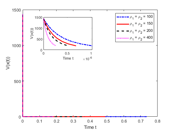
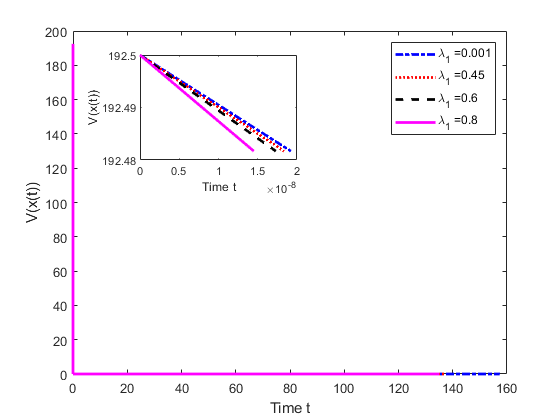
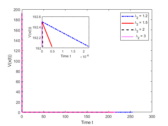
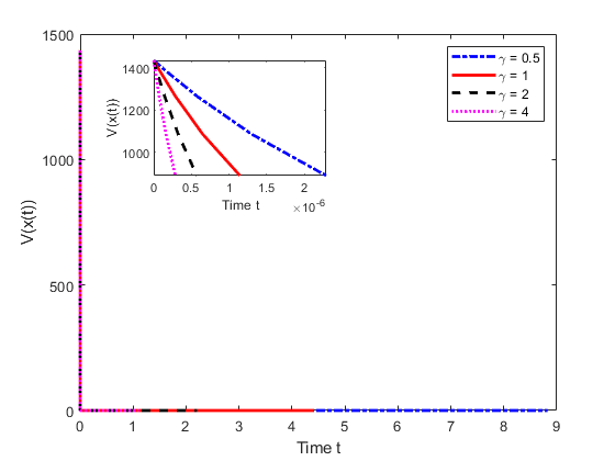
It follows from [32] that the smaller settling-time often implies the faster convergent rate of a given fixed-time dynamical system. Hence, it concludes from (3.2), (3.3) and (3.4) that the larger γ\gamma, ρ1\rho_{1} or ρ2\rho_{2} is, the smaller the upper bound TmaxT_{\max} of the settling-time or the faster convergence rate of the dynamical system (3.1) is. In addition, TmaxT_{\max} is also dependent on the parameters λ1\lambda_{1} and λ2\lambda_{2}. See the next section for more details.

4 Numerical simulations

In this section, we will present one example to illustrate the effectiveness of the proposed method. All experiments are implemented in MATLAB R2018b with a machine precision 2.22×10162.22\times 10^{-16} on a PC Windows 10 operating system with an Intel i7-9700 CPU and 8GB RAM. The ODE solver used is “ode23”. Concretely, the MATLAB expression

[t,y]=ode23(odefun,tspan,y0)[t,y]=\text{ode23}(odefun,tspan,y_{0})

is used, which integrates the system of differential equations from t0t_{0} to tft_{f} with tspan=[t0,tf]tspan=[t_{0},t_{f}]. Here, “odefun” is a function handle.

Example 4.1 (​​[5]).

Consider the AVEs (1.1) with

A=tridiag(1,8,1)n×nandb=Ax|x|,A=\textbf{tridiag}(-1,8,-1)\in\mathbb{R}^{n\times n}\quad\text{and}\quad b=Ax^{*}-|x^{*}|,

where x=(1,1,1,1,,1,1)n.x^{*}=(-1,1,-1,1,\cdots,-1,1)^{\top}\in\mathbb{R}^{n}.

In this example, we have A1<1\|A^{-1}\|<1 and thus the AVEs (1.1) has a unique solution for any bnb\in\mathbb{R}^{n}. Equivalently, the dynamical model (3.1) has a unique equilibrium point and it is globally fixed-time stable.

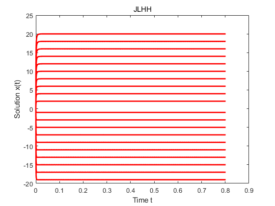
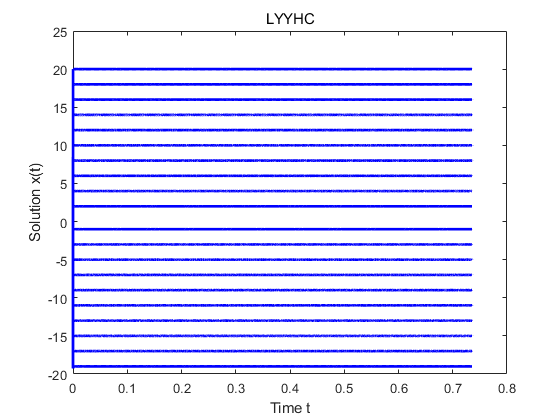
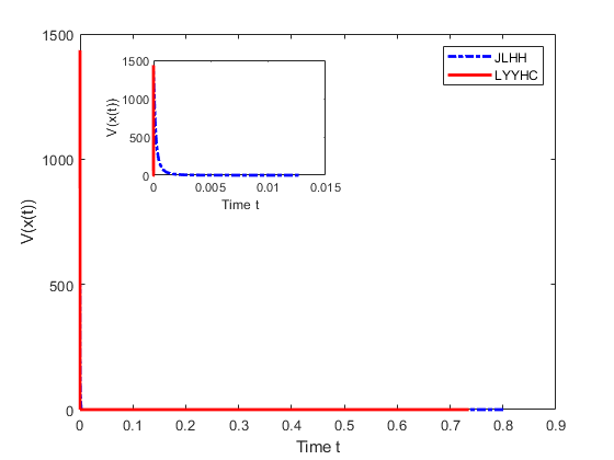
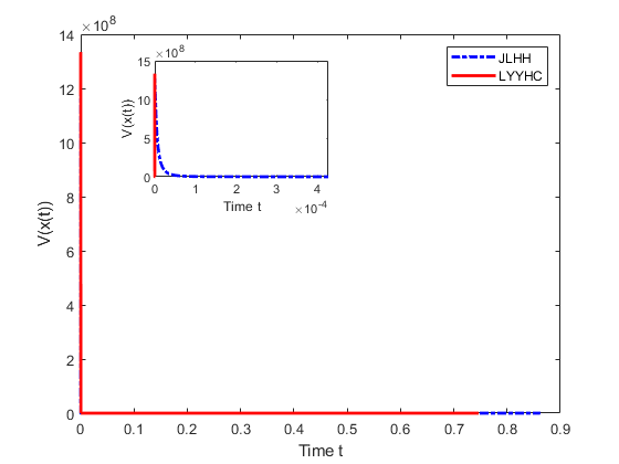
Since we are interested in the fixed-time stable dynamical systems, in the first stage, we only compare our method (denoted by ‘LYYHC’) with the method (denoted by ‘JLHH’) proposed in [11]. For both methods, we set ρ1=ρ2=100\rho_{1}=\rho_{2}=100, λ1=0.5\lambda_{1}=0.5, λ2=1.5\lambda_{2}=1.5. For LYYHC, γ=6\gamma=6 and x=(0,0,,0)n.x^{*}=(0,0,\cdots,0)^{\top}\in\mathbb{R}^{n}. For JLHH, θ=0.5λmin(M)\theta=0.5*\lambda_{\min}(M), η\eta is selected such that ηL2<2θ\eta L^{2}<2\theta and y0=(MI)x0by_{0}=(M-I)x_{0}-b. When n=20n=20, we have η=1.2,θ=1.2228,TmaxJLHH=0.8015,TmaxLYYHC=0.7355\eta=1.2,\theta=1.2228,T_{\max}^{JLHH}=0.8015,T_{\max}^{LYYHC}=0.7355 and numerical simulations are shown in Figure 1 and Figure 2. When n=2000n=2000, we have η=1.2,θ=1.2222,TmaxJLHH=0.8625,TmaxLYYHC=0.7467\eta=1.2,\theta=1.2222,T_{\max}^{JLHH}=0.8625,T_{\max}^{LYYHC}=0.7467 and numerical simulations are shown in Figure 2. Under the setting of these parameters, numerical results show that LYYHC is superior to JLHH.

In the second stage, we show the influence of the tunable parameters for LYYHC. Firstly, we fix γ=6,λ1=0.5,λ2=1.5,n=20\gamma=6,\lambda_{1}=0.5,\lambda_{2}=1.5,n=20. Secondly, we freeze γ=1,ρ1=ρ2=2,λ1=0.5,n=10\gamma=1,\rho_{1}=\rho_{2}=2,\lambda_{1}=0.5,n=10. Thirdly, we fix γ=5,ρ1=ρ2=5,λ2=1.01,n=10\gamma=5,\rho_{1}=\rho_{2}=5,\lambda_{2}=1.01,n=10. Finally, we set ρ1=ρ2=100,λ1=0.5,λ2=1.5,n=20\rho_{1}=\rho_{2}=100,\lambda_{1}=0.5,\lambda_{2}=1.5,n=20 and alter γ\gamma. Numerical results are shown in Figure 3 and Table 1, for this example, from which we can observe that the settling-time of LYYHC is decreasing with increased value of parameters γ,ρ1,ρ2\gamma,\rho_{1},\rho_{2}. However, the influence of the parameters λ1\lambda_{1} and λ2\lambda_{2} on TmaxT_{\max} or the convergence rate of (3.1) is more complicated.

Refer to caption
Refer to caption
Figure 1: Phase diagrams for Example 4.1 with n=20n=20.
Refer to caption
Refer to caption
Figure 2: The energy V(x(t))V(x(t)) for Example 4.1 with n=20n=20 (left) and n=2000n=2000 (right). The energy of the first 3030 points in the trajectory is shown in the inner figure, from which we clearly see that LYYHC converges faster than LJHH.
Refer to caption
Refer to caption
Refer to caption
Refer to caption
Figure 3: The energy V(x(t))V(x(t)) for Example 4.1 with different parameters.
Table 1: TmaxT_{\max} for Example 4.1.
λ1\lambda_{1} 0.0010.001 0.450.45 0.60.6 0.80.8
TmaxT_{\max} 157.3289157.3289 137.0701137.0701 134.7652134.7652 135.0736135.0736
λ2\lambda_{2} 1.21.2 1.51.5 22 33
TmaxT_{\max} 254.8676254.8676 212.1412212.1412 203.5690203.5690 219.5776219.5776
γ\gamma 0.50.5 11 22 44
TmaxT_{\max} 8.82648.8264 4.41324.4132 2.20662.2066 1.10331.1033
ρ1(orρ2)\rho_{1}(\text{or}~{}\rho_{2}) 100100 150150 200200 400400
TmaxT_{\max} 0.73550.7355 0.49040.4904 0.36780.3678 0.18390.1839

5 Conclusion

In this paper, a fixed-time dynamical system is proposed to solve the AVEs (1.1). Theoretical results show that the presented model is globally convergent and has a conservative settling-time. Numerical comparison with the method proposed in [11] shows that our method is preferred, at least in the sense that our method is inverse-free.

References

  • [1] S. P. Bhat, D. S. Bernstein. Finite-time stability of continuous autonomous ststems, SIAM J. Control Optim., 38: 751–766, 2000.
  • [2] C.-R. Chen, Y.-N. Yang, D.-M. Yu, D.-R. Han. An inverse-free dynamical system for solving the absolute value equations, Appl. Numer. Math., 168: 170–181, 2021.
  • [3] X.-B. Gao. A neural network for a class of extended linear variational inequalities, Chin. J. Electron., 10: 471–475, 2001.
  • [4] X.-B. Gao, J. Wang. Analysis and application of a one-layer neural network for solving horizontal linear complementarity problems, Int. J. Conput. Int. Sys., 7: 724–732, 2014.
  • [5] P. Guo, S.-L Wu, C.-X Li. On the SOR-like iteration method for solving absolute value equations, Appl. Math. Lett., 97: 107–113, 2019.
  • [6] M. Hladík. Bounds for the solutions of absolute value equations, Comput. Optim. Appl., 69: 243–266, 2018.
  • [7] M. Hladík, H. Moosaei. Some notes on the solvability conditions for absolute value equations, Optim. Lett., 2022. https://doi.org/10.1007/s11590-022-01900-x.
  • [8] S.-L. Hu, Z.-H. Huang. A note on absolute value equations, Optim. Lett., 4: 417–424, 2010.
  • [9] X.-L. Hu, J. Wang. A recurrent neural network for solving a class of general variational inequalities, IEEE Trans. Syst., Man, Cybern. B, Cybern., 37: 528–539, 2007.
  • [10] X.-J. Huang, B.-T. Cui. Neural network-based method for solving absolute value equations, ICIC-EL, 11: 853–861, 2017.
  • [11] X.-X. Ju, C.-D. Li, X. Han, X. He. Neurodynamic network for absolute value equations: A fixed-time convergence technique, IEEE T. Circuits-II, 69: 1807–1811, 2022.
  • [12] H.K. Khalil. Nonlinear Systems, Prentice-Hall, Michigan, NJ, 1996.
  • [13] Q.-S. Liu, J.-D. Cao. A recurrent neural network based on projection operator for extended general variational inequalities, IEEE Trans. Syst., Man, Cybern. B, Cybern., 40: 928–938, 2010.
  • [14] O.L. Mangasarian. Absolute value programming, Comput. Optim. Appl., 36: 43–53, 2007.
  • [15] O.L. Mangasarian. Knapsack feasibility as an absolute value equation solvable by successive linear programming, Optim. Lett., 3: 161–171, 2009.
  • [16] O.L. Mangasarian, R.R. Meyer. Absolute value equations, Linear Algebra Appl., 419: 359–367, 2006.
  • [17] A. Mansoori, M. Erfanian. A dynamic model to solve the absolute value equations, J. Comput. Appl. Math., 333: 28–35, 2018.
  • [18] A. Mansoori, M. Eshaghnezhad, S. Effati. An efficient neural network model for solving the absolute value equations, IEEE T. Circuits-II, 65: 391–395, 2017.
  • [19] F. Mezzadri. On the solution of general absolute value equations, Appl. Math. Lett., 107: 106462, 2020.
  • [20] A. Polyakov. Nonlinear feedback design for fixed-time stabilization of linear control systems, IEEE Trans. Autom. Control, 57: 2106–2110, 2011.
  • [21] O. Prokopyev. On equivalent reformulations for absolute value equations, Comput. Optim. Appl., 44: 363–372, 2009.
  • [22] J. Rohn. Systems of linear interval equations, Linear Algebra Appl., 126: 39–78, 1989.
  • [23] J. Rohn. A theorem of the alternatives for the equation Ax+B|x|=bAx+B|x|=b, Linear Multilinear Algebra, 52: 421–426, 2004.
  • [24] J. Rohn, V. Hooshyarbakhsh, R. Farhadsefat. An iterative method for solving absolute value equations and sufficient conditions for unique solvability, Optim. Lett., 8: 35–44, 2014.
  • [25] B. Saheya, C. T. Nguyen, J.-S. Chen. Neural network based on systematically generated smoothing functions for absolute value equation, J. Appl. Math. Comput., 61: 533–558, 2019.
  • [26] F.-R. Wang, Z.-S. Yu, C. Gao. A smoothing neural network algorithm for absolute value equations, Engineering, 7: 567–576, 2015.
  • [27] S.-L. Wu, P. Guo. On the unique solvability of the absolute value equation, J. Optim. Theory Appl., 169: 705–712, 2016.
  • [28] S.-L. Wu, C.-X. Li. The unique solution of the absolute value equations, Appl. Math. Lett., 76: 195–200, 2018.
  • [29] Y. Xia, J. Wang. A general projection neural network for solving monotone variational inequalities and related optimization problems, IEEE Trans. Neural Netw., 15: 318–328, 2004.
  • [30] L.-Q. Yong. Neural network method for absolute value equation and linear complementarity problem, Journal of Shaanxi University of Technology (Natural Science Edition), 36: 72–81, 2020 (in Chinese).
  • [31] D.-M. Yu, C.-R. Chen, Y.-N. Yang, D.-R. Han. An inertial inverse-free dynamical system for solving absolute value equations, J. Ind. Manag. Optim., 2022. doi:10.3934/jimo.2022055.
  • [32] Z. Zuo, Q.-L. Han, B. Ning, X. Ge, X.-M. Zhang. An overview of recent advances in fixed-time cooperative control of multiagent systems, IEEE Trans. Ind. Informat., 14: 2322–2334, 2018.