A Fourier transform method for spread option pricing††thanks: Research supported by the Natural Sciences and Engineering Research Council of Canada and MITACS, Mathematics of Information Technology and Complex Systems Canada
Abstract
Spread options are a fundamental class of derivative contract written on multiple assets, and are widely used in a range of financial markets. There is a long history of approximation methods for computing such products, but as yet there is no preferred approach that is accurate, efficient and flexible enough to apply in general models. The present paper introduces a new formula for general spread option pricing based on Fourier analysis of the spread option payoff function. Our detailed investigation proves the effectiveness of a fast Fourier transform implementation of this formula for the computation of prices. It is found to be easy to implement, stable, efficient and applicable in a wide variety of asset pricing models.
Keywords: Spread options, multivariate spread options, jump-diffusions, fast Fourier transform, gamma function.
AMS Subject Classification: 33B15, 65T50, 91B28
1 Introduction
When are two asset price procsses, the basic spread option with maturity and strike is the contract that pays at time . From the risk-neutral expectation formula, the time price of this option, assuming a constant interest rate , must be
| (1) |
The literature on applications of spread options is extensive, and is reviewed by Carmona and Durrleman [1] who explore further applications of spread options beyond the case of equities modelled by geometric Brownian motion, notably energy trading. For example, the “crack spread” is the difference between the prices of crude oil and natural gas. “Spark spreads” refer to differences between the price of electricity and the price of fuel: options on spark spreads are widely used by power plant operators to optimize their revenue streams. Energy pricing requires models with mean reversion and jumps very different from geometric Brownian motion, and pricing spread options in such situations can be challenging.
Closed formulas for (1) are known only for a limited set of cases. In the Bachelier stock model, is an arithmetic Brownian motion, and in this case (1) has a Black-Scholes type formula for any . In the special case when is geometric Brownian motion, (1) is given by the Margrabe formula [8].
In the important case where is geometric Brownian motion and , no explicit pricing formula is known. Therefore there is a long history of approximation methods. Numerical integration methods, typically Monte Carlo based, are often employed. Dempster and Hong [4] introduced a numerical integration method based on double fast Fourier transforms (FFT) that is efficient for geometric Brownian motion and certain more general asset price processes.
Another stream of research develops analytical methods applicable to log normal models that involve linear approximations of the nonlinear exercise boundary. Such methods are often very fast, but their accuracy is usually not easy to determine. Kirk [5] presented an analytical approximation that performs well in practice. Carmona and Durrleman [2] used a family of lower bounds for the spread option price to obtain an analytical approximation formula that apparently leads to acceptable accuracy. Moreover these results extend to approximate values for the Greeks. Deng, Li and Zhou [6] have developed a systematic analytical approximation scheme which is perhaps even more reliable.
Next to having analytical option pricing formulas, the fastest option pricing engines by numerical integration are usually those based on the fast Fourier transform methods introduced by Carr and Madan [3]. Their interest was in option pricing for geometric Lévy process models like the variance gamma (VG) model, but their basic framework has been adapted to a host of other models where the characteristic function of the returns is known.
The main purpose of the present paper is to give a new numerical integration method for computing spread options in two or higher dimensions via FFTs, applicable to any model for which the characteristic function of the joint return process is given analytically. Our method is completely different from prior approaches, and consequently has distinct advantages, notably the flexibility to include a wide range of desirable asset return models, with a competitive computational expense.
The results we describe all stem from the following fundamental new result that gives a Fourier representation of the basic spread option payoff function . Note that this spread option payoff is without loss of generality: We can reduce the general case to by using scaling and interchange of and .
Theorem 1.
For any real numbers with and
| (2) |
Here is the complex gamma function defined for by the integral . We write and and the notation denotes the (unconjugated) matrix transpose.
Using this result, whose proof is given in the appendix, we will find we can follow the logic of Carr and Madan to derive numerical algorithms for efficient computation of a variety of spread options and their Greeks. The basic strategy to compute (1) is to combine (2) with an explicit formula for the characteristic function of the bivariate random variable . For the remainder of this paper, we make a simplifying assumption that the dynamics of is homogeneous, which is equivalent to the following factorization of the characteristic function
| (3) |
Then, if is the price process for two traded assets, the spread option formula can be written
| (4) | |||||
The Greeks are handled in exactly the same way. For example, the Delta is obtained as a function of by replacing in (4) by .
Explicit double Fourier integrals like this can be approximated numerically by a two dimensional FFT. Such approximations involve both a truncation and discretization of the integral, and the two properties that determine their accuracy are the decay of the integrand of (4) in -space, and the decay of the function Spr in -space. The remaining issue of computing the gamma function is not a real difficulty. Fast and accurate computation of the complex gamma function in for example, Matlab, is based on the Lanczos approximation popularized by [9]111According to these authors, computing the gamma function becomes “not much more difficult than other built-in functions that we take for granted, such as or ”..
In this paper, we demonstrate how our method performs in three different models for spread options on two stocks, namely the geometric Brownian motion (GBM), a three factor stochastic volatility (SV) model and the variance gamma (VG) model. Section 2 provides the essential definitions of the three types of models, including explicit formulas for their bivariate characteristic functions. Section 3 discusses how the two dimensional FFT can be implemented for our problem, and gives a heuristic picture of how the accuracy and speed will depend on the choices made in the implementation. Section 4 gives the detailed results of the performance of the method in the three models. In that section, the accuracy of each model is compared to benchmark values computed by an independent method for a reference set of option prices. We also demonstrate that the computation of the spread option Greeks in such models is equally feasible. Section 5 extends all the above results to spread options on three or more assets. While in such cases the formulation is simple, the resulting higher dimensional FFTs are in practice much slower to compute.
2 Three kinds of stock models
2.1 The case of geometric Brownian motion
In the two-asset Black-Scholes model, the vector has components
where and are risk-neutral Brownian motions with constant correlation . The joint characteristic function of as a function of is of the form with
| (5) |
where and . Here we use implied matrix multiplication, and the denotes the (unconjugated) matrix transpose. Substituting this expression into (4) yields the spread option formula
| (6) |
As we discuss in Section 3, we recommend that this be computed numerically using the FFT.
2.2 Three Factor Stochastic Volatility Model
The spread option problem in a three factor stochastic volatility model was given as an example by Dempster and Hong [4]. Their model is defined by the SDE for :
where
As discussed in that paper, it has the joint characteristic function where
where
2.3 Exponential Lévy Models
Many stock price models are of the form where is a Lévy process for which the characteristic function is explicitly known. We illustrate with example of the VG process introduced by [7], the three parameter process with Lévy characteristic triple where the Lévy measure is for positive constants . The characteristic function of is
| (7) |
To demonstrate the effects of correlation, we take a bivariate VG model driven by three independent VG processes with common parameters and . The bivariate log return process is a mixture:
| (8) |
Here leads to dependence between the two return processes, but leaves their marginal laws unchanged. An easy calculation leads to the bivariate characteristic function with
3 Numerical Integration by Fast Fourier Transform
To compute (4) in these models we approximate the double integral by a double sum over the lattice
for appropriate choices of For the FFT it is convenient to take to be a power of and lattice spacing such that truncation of the -integrals to and discretization leads to an acceptable error. Finally, we choose initial values to lie on the reciprocal lattice with spacing :
For any with we then have the approximation
| (10) |
Now, as usual for the discrete FFT, as long as is even,
This leads to the double inverse discrete Fourier transform
| (11) | |||||
where
The selection of suitable values for and is a somewhat subtle issue when implementing the above FFT approximation of (4). We now briefly discuss separately the truncation error and discretization error. The pure truncation error, defined by taking keeping fixed, can be made small if the integrand of (4) is small outside the square . Corollary 4, proved in the Appendix, gives an upper bound on , while can generally been seen directly to have some -decay. Typically, with some caveats, if one picks large enough so that and has decay outside the square, then the truncation error will be less than .
The pure discretization error, defined by taking while keeping fixed, can be made small if , taken as a function of , has rapid decay in . This is related to the smoothness of and the choice of . The first two models are not very sensitive to , but in the VG model the following conditions are needed to ensure that singularities in space are avoided:
The error in the approximation (11) with and finite, is given by the formula
Typically, with some caveats, the norm of this can be made smaller than for if and is and rapidly decaying outside the square .
In summary, one expects that the combined truncation and discretization error will be if and are each chosen as above.
The FFT method can also be applied to the Greeks, enabling us to tackle hedging and other interesting problems. It is particularly efficient for the GBM model, where differentiation under the integral sign is always permissible. For instance, the FFT formula for vega (the sensitivity to ) takes the form:
where and . Other Greeks including those of higher orders can be computed in similar fashion. This method needs to be used with care for the SV and VG models, since it is possible that differentiation leads to an integrand that decays slowly.
4 Numerical Results
Our numerical experiments were coded and implemented in Matlab version 7.6.0 on an Intel 2.80 GHz machine running under Linux with 1 GB physical memory. If they were coded in C++ with similar algorithms, we should expect to see much faster performance. All the following experiments were run with .
The strength of the FFT method is demonstrated by comparison with benchmarks. Based on a selection of , the objective function we measure is defined as
| (12) |
where and are FFT computed prices and benchmark prices for the combination. We chose and fixed the strike , leading to 36 prices contributing to the objective function. These choices cover a wide range of moneyness, from deep out-of-the-money to deep in-the-money. Since these combinations all lie on lattices corresponding to and for integers , all 36 prices can be computed simultaneously with one FFT.
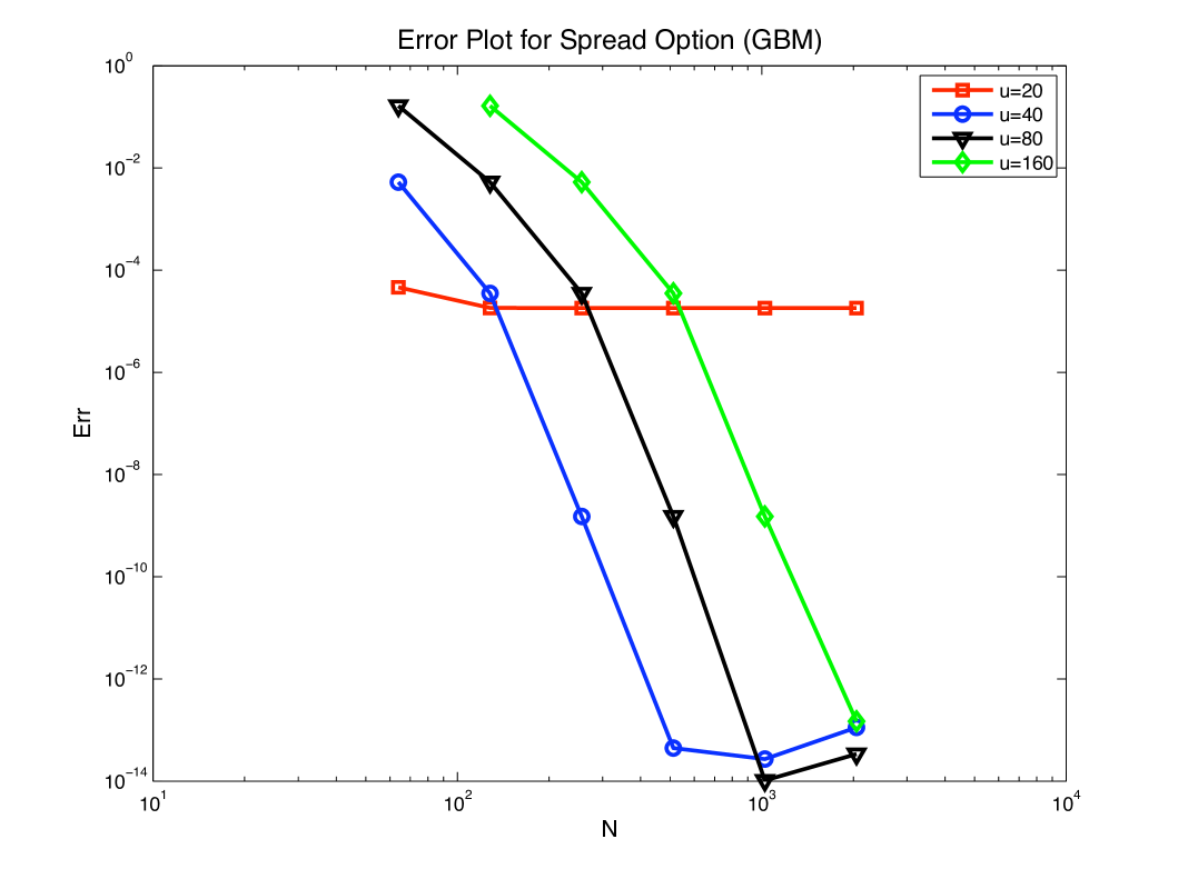
Figure 1 shows how the FFT method performs in the 2-dimensional Geometric Brownian motion model for different choices of and . Since the two factors are bivariate normal, benchmark prices can be calculated to high accuracy by one dimensional integrations. In Figure 1 we can clearly see the effects of both truncation errors and discretization errors. For a fixed , the objective function decreases when increases. The curve flattens out near due to its truncation error of that magnitude. In turn, we can quantify its discretization errors with respect to by subtracting the truncation error from the total error. The flattening of the other three curves near should be attributed to Matlab round-off errors: because of the rapid decrease of the characteristic function , their truncation error is negligible. For a fixed , increasing brings two effects: reducing truncation error and enlarging discretization error. These effects are well demonstrated in figure 1.
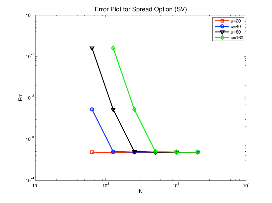
For the stochastic volatility model, no analytical or numerical method we know is consistently more accurate to serve as benchmark. Instead, we used Monte Carlo simulation to achieve a moderate degree of accuracy. Each benchmark price was created by simulations, each consisting of 2000 time steps. No variance reduction was employed. The resulting objective function is shown in Figure 2. The objective function only decreases to near , reflecting the inaccuracy of the benchmark. A comparable graph (not shown), using benchmark prices computed with the FFT method with and , showed similar behaviour to Figure 1, and is consistent with accuracies at the level of round-off. The computational cost to reduce the Monte Carlo simulation error to a comparable level would be prohibitive.
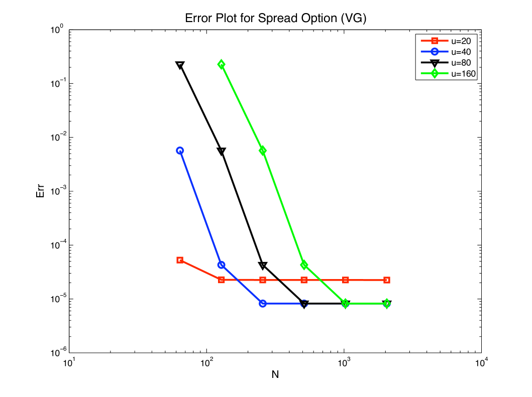
The VG model also lacks a reliable benchmark, so again we used Monte Carlo simulation. Since the VG process can be simulated as a Brownian motion time-changed by a gamma process, MC is here much more efficient than for the SV model, and we were able to run simulations with antithetic variates for each price. The objective function is shown in Figure 3. The truncation error for is about . The other three curves flatten out near , which is presumably the accuracy of the benchmark. A comparable graph (not shown), using benchmark prices computed with the FFT method with and , showed similar behaviour to Figure 1, and is consistent with the FFT method being capable of producing accuracies at the level of round-off.
The strength of the FFT method is further illustrated by the computation of individual prices shown in Tables 1 to 3. The columns labeled “Analytic” and “Simulation” refer to the type of benchmark used. One can observe that an FFT with is capable of producing very high accuracy in all three models. In the GBM model, the errors are simply due to round-off. The discrepancies in the VG model are small too, less than 1 basis point. The apparent discrepancies in the SV model we attribute to the inaccurate benchmark, rather than the FFT method itself.
| Strike K | Analytic | 64 | 128 | 256 | 512 |
|---|---|---|---|---|---|
| 0.4 | 8.312461 | 8.206666 | 8.312331 | 8.312461 | 8.312461 |
| 0.8 | 8.114994 | 8.009643 | 8.114864 | 8.114994 | 8.114994 |
| 1.2 | 7.920820 | 7.815913 | 7.920691 | 7.920820 | 7.920820 |
| 1.6 | 7.729932 | 7.625469 | 7.729804 | 7.729932 | 7.729932 |
| 2.0 | 7.542324 | 7.438304 | 7.542196 | 7.542324 | 7.542324 |
| 2.4 | 7.357984 | 7.254408 | 7.357857 | 7.357984 | 7.357984 |
| 2.8 | 7.176902 | 7.073770 | 7.176775 | 7.176902 | 7.176902 |
| 3.2 | 6.999065 | 6.896377 | 6.998939 | 6.999065 | 6.999065 |
| 3.6 | 6.824458 | 6.722213 | 6.824332 | 6.824458 | 6.824458 |
| 4.0 | 6.653065 | 6.551264 | 6.652940 | 6.653065 | 6.653065 |
| Strike K | 64 | 128 | 256 | 512 | Interpolation | Simulation |
|---|---|---|---|---|---|---|
| 2.0 | 6.996467 | 7.544853 | 7.548502 | 7.548502 | 7.548502 | 7.545784 |
| 2.2 | 6.902676 | 7.449895 | 7.453536 | 7.453536 | 7.453536 | 7.435475 |
| 2.4 | 6.809696 | 7.355748 | 7.359381 | 7.359381 | 7.359381 | 7.360184 |
| 2.6 | 6.717527 | 7.262411 | 7.266036 | 7.266037 | 7.266036 | 7.276051 |
| 2.8 | 6.626167 | 7.169883 | 7.173501 | 7.173501 | 7.173501 | 7.193546 |
| 3.0 | 6.535616 | 7.078165 | 7.081775 | 7.081775 | 7.081775 | 7.077421 |
| 3.2 | 6.445873 | 6.987254 | 6.990856 | 6.990857 | 6.990856 | 6.983995 |
| 3.4 | 6.356936 | 6.897150 | 6.900745 | 6.900745 | 6.900745 | 6.913994 |
| 3.6 | 6.268806 | 6.807853 | 6.811439 | 6.811440 | 6.811439 | 6.818526 |
| 3.8 | 6.181481 | 6.719360 | 6.722939 | 6.722939 | 6.722939 | 6.735112 |
| 4.0 | 6.094959 | 6.631670 | 6.635241 | 6.635242 | 6.635241 | 6.621617 |
| Strike K | 64 | 128 | 256 | 512 | Interpolation | Simulation |
|---|---|---|---|---|---|---|
| 2.0 | 9.157674 | 9.723691 | 9.727458 | 9.727458 | 9.727458 | 9.727546 |
| 2.2 | 9.061487 | 9.626247 | 9.630006 | 9.630006 | 9.630006 | 9.629444 |
| 2.4 | 8.965876 | 9.529448 | 9.533200 | 9.533200 | 9.533200 | 9.533137 |
| 2.6 | 8.870896 | 9.433296 | 9.437040 | 9.437040 | 9.437040 | 9.437323 |
| 2.8 | 8.776560 | 9.337792 | 9.341527 | 9.341528 | 9.341527 | 9.341547 |
| 3.0 | 8.682870 | 9.242934 | 9.246662 | 9.246662 | 9.246662 | 9.246273 |
| 3.2 | 8.589828 | 9.148725 | 9.152445 | 9.152445 | 9.152445 | 9.152956 |
| 3.4 | 8.497433 | 9.055163 | 9.058875 | 9.058875 | 9.058875 | 9.058997 |
| 3.6 | 8.405687 | 8.962250 | 8.965954 | 8.965954 | 8.965954 | 8.966410 |
| 3.8 | 8.314590 | 8.869984 | 8.873681 | 8.873681 | 8.873681 | 8.874129 |
| 4.0 | 8.224140 | 8.778368 | 8.782057 | 8.782057 | 8.782057 | 8.781863 |
The FFT computes in a single iteration an panel of prices corresponding to initial values , , , (. If the desired selection of fits into this panel of prices, or its scaling, a single FFT suffices. If not, then one has to match () with each combination, and run several FFTs, with a consequent increase in computation time. However, we have found that an interpolation technique is very accurate for practical purposes. For instance, prices for multiple strikes with the same and are approximated by a polynomial fit along the diagonal of the price panel: , , . The results of this technique are recorded in Table 2 and Table 3 in the column “Interpolation”. We can see this technique generates very competitive results and moreover, saves computational resource.
Finally, we computed first order Greeks using the method described at the beginning of Section 3 and compared them with finite differences. As seen in Table 4, the two methods come up with very consistent results. The Greeks of our at-the-money spread option exhibit some resemblance to the at-the-money European put/call option. The delta of is close to the delta of the call option, which is about 0.5. And the delta of is close to the delta of the put option, which is also about 0.5. The time premium of the spread option is positive. The option price is much more sensitive to volatility than to volatility. It is an important feature that the option price is negatively correlated with the underlying correlation: Intuitively speaking, if the two underlyings are strongly correlated, their co-movements diminish the probability that develops a wide spread over . This result is consistent with observations made by [6].
| Delta(S1) | Delta(S2) | Theta | Vega() | Vega() | ||
|---|---|---|---|---|---|---|
| FD | 0.512648 | -0.447127 | 3.023823 | 33.114315 | -0.798959 | -4.193749 |
| FFT | 0.512705 | -0.447079 | 3.023777 | 33.114834 | -0.798972 | -4.193728 |
Since the FFT method naturally generates a panel of prices, and interpolation can be implemented accurately with negligible additional computational cost, it is appropriate to measure the efficiency of the method by timing the computation of a panel of prices. Such computing times are shown in Table 5. For the FFT method, the main computational cost comes from the calculation of the matrix in (11) and the subsequent FFT of . We see that the GBM model is noticeably faster than the SV and VG models: This is due to a recursive method used to calculate the matrix entries of the GBM model, which is not applicable for the SV and VG models. The number of calculations for is of order which for large exceeds the of the FFT of , and thus the advantage of this efficient algorithm for GBM is magnified as increases. However, our FFT method is still very fast for the SV and VG models and is able to generate a large panel of prices within a couple of seconds.
| Discretization | GBM | SV | VG |
|---|---|---|---|
| 64 | 0.091647 | 0.083326 | 0.109537 |
| 128 | 0.099994 | 0.120412 | 0.139276 |
| 256 | 0.126687 | 0.234024 | 0.220364 |
| 512 | 0.240938 | 0.711395 | 0.621074 |
| 1024 | 0.609860 | 2.628901 | 2.208770 |
| 2048 | 2.261325 | 10.243228 | 8.695122 |
5 High Dimensional Spread Options
The ideas of section 2 turn out to extend naturally to basket options with payoffs for . The analysis is based on a simple result proved in the Appendix:
Proposition 2.
Let and with for all . Then
| (13) |
As before we write and seek to compute for ,
We introduce the factor and interchange the integral with the integrals. Then using Proposition 2 one finds
When we can apply Proposition 1, we obtain the result:
Proposition 3.
For any real numbers with for all and
| (14) |
where
| (15) |
6 Conclusion
This paper presents a fundamentally new approach to the valuation of spread options, an important class of financial contracts. The method is based on a newly discovered explicit formula for the Fourier transform of the spread option payoff in terms of the gamma function.
This mathematical result leads to simple and transparent algorithms for computing spread options in all dimensions. The powerful tool of the Fast Fourier Transform provides an accurate and efficient implementation of the fundamental result. The difficulties and pitfalls of the FFT, of which there are admittedly several, are by now well understood, and thus the reliability and stability properties of our method are rather clear.
Many important processes in finance, particularly affine models and Lévy jump models, have well known explicit characteristic functions, and can be included in the method with little difficulty. Thus the method can be easily applied to important problems arising in energy and commodity markets.
Finally, the Greeks can be systematically evaluated for such models, with similar performance and little extra work.
Appendix A Proof of Theorem 1 and Proposition 2
Proof of Theorem 1: Suppose . One can then verify either directly or from the argument that follows that is in . Therefore, application of the Fourier inversion theorem to implies that
| (16) |
where
By restricting to the domain we have
The change of variables then leads to
The beta function
is defined for any complex with by
From this, and the property follow the formulas
| (17) |
The above derivation also leads to the following bound on .
Corollary 4.
Fix for some . Then
| (18) |
where .
Proof: First note that for , . Then (17) and a symmetric formula with leads to the upper bound
But since is monotonic and for all , the required result follows.
Proof of Proposition 2: To simplify the proof, we make the change of variables and . It becomes to prove that
| (19) |
We prove the proposition by induction. The above equation trivially holds when . Now suppose it holds for . Then for
| (20) | |||||
The above step makes use of the result when . The proof is then complete when one notices that the integral is simply multiplied by a beta function with parameters and .
References
- [1] R. Carmona and V. Durrleman, Pricing and hedging spread options, SIAM Review, 45 (2003), pp. 627–685.
-
[2]
, Pricing and hedging
spread options in a log-normal model, tech. report, Princeton University,
2003.
Available at
orfe.princeton.edu/~rcarmona/download/fe/spread.pdf. - [3] P. Carr and D. Madan, Option valuation using the fast Fourier transform, Journal of Computational Finance, 2 (2000).
-
[4]
M. A. H. Dempster and S. S. G. Hong, Spread option valuation and the
fast Fourier transform. manuscript, tech. report, Cambridge University,
2000.
Available at
www.jbs.cam.ac.uk/research/working_papers/2000/wp0026.pdf. - [5] E. Kirk, Correlations in the energy markets, in In Managing Energy Price Risk, Risk Publications and Enron, London, 1995, pp. 71–78.
- [6] M. Li, S. Deng, and J. Zhou, Closed-form approximations for spread option prices and greeks. Available at SSRN: http://ssrn.com/abstract=952747, 2006.
- [7] D. Madan and E. Seneta, The VG model for share market returns, Journal of Business, 63 (1990), pp. 511–524.
- [8] William Margrabe, The value of an option to exchange one asset for another, Journal of Finance, 33 (1978), pp. 177–86.
- [9] W. H. Press, S. A. Teukolsky, W. T. Vetterling, and B. P. Flannery, Numerical Recipes 3rd Edition: The Art of Scientific Computing, Cambridge University Press, 2007.