A free boundary problem for semi-linear elliptic equation and its applications^∗

Jianfeng Cheng^1,2, Lili Du²

Abstract.

In this paper, we consider a free boundary problem of a semilinear nonhomogeneous elliptic equation with Bernoulli’s type free boundary. The existence and regularity of the solution to the free boundary problem are established by use of the variational approach. In particular, we establish the Lipschitz continuity and non-degeneracy of a minimum, and regularity of the free boundary. As a direct and important application, the well-posedness results on the steady, incompressible inviscid jet and cavitational flow with general vorticity are also obtained in this paper.

^∗This work is supported in part by NSFC grant 11971331.

E-Mail: jianfengcheng@126.com (J. Cheng), E-mail: dulili@scu.edu.cn (L. Du).

¹ The Institute of Mathematical Sciences,

The Chinese University of Hong Kong, Hong Kong.

² Department of Mathematics, Sichuan University,

Chengdu 610064, P. R. China.

2010 Mathematics Subject Classification: 76B10; 76B03; 35Q31; 35J25.

Key words: Semilinear elliptic equation; Free boundary; Regularity; Incompressible flow; General vorticity.

1. Introduction

In this paper, we investigate the free boundary problem of a semilinear nonhomogeneous elliptic equation

\left\{\begin{array}[]{ll}-\Delta\psi=f(\psi)&\text{in}\ \ \Omega\cap\{\psi>0\},\\ |\nabla\psi|=\lambda(X)&\text{on}\ \ \Omega\cap\partial\{\psi>0\},\\ \psi=\Psi_{0}&\text{on}\ \ \partial\Omega,\end{array}\right.

(1.1)

where $\displaystyle\Omega$ is a connected open and bounded domain in $\displaystyle\mathbb{R}^{2}$ , $\displaystyle\partial\Omega$ is a local Lipschitz graph. The given functions $\displaystyle\Psi_{0}\in C^{0,1}(\bar{\Omega})$ with $\displaystyle\Psi_{0}\geq 0$ and $\displaystyle\lambda(X)\in C^{0,\beta}(\bar{\Omega})$ with $\displaystyle 0<\lambda_{1}\leq\lambda(X)\leq\lambda_{2}<+\infty$ , $\displaystyle f(\psi)$ is so-called vorticity strength function and $\displaystyle f\in C^{1,\beta}(\mathbb{R})$ , $\displaystyle 0<\beta<1$ .

The semilinear nonhomogeneous equation $\displaystyle-\Delta\psi=f(\psi)$ characterizes the steady, incompressible flow of an ideal fluid in $\displaystyle\mathbb{R}^{2}$ with non-zero variable vorticity. A wide class of vorticity distributions is considered. We are interesting in the existence, regularity and geometric properties of the solution $\displaystyle\psi$ and the free boundary $\displaystyle\Omega\cap\partial\{\psi>0\}$ .

On the other hand, physical motivation for our study lies in the proof of minimizing the functional

J(\psi)=\int_{\Omega}|\nabla\psi|^{2}+F(\psi)+\lambda^{2}(X)I_{\{\psi>0\}}dX,

which is related closely to the jet flow problem with variable vorticity. Here, $\displaystyle F(t)=-2\int_{0}^{t}f(s)ds$ , $\displaystyle I_{E}$ is the characteristic function of the set $\displaystyle E$ . Here and after, denote $\displaystyle dX=dxdy$ for simplicity.

In the remarkable paper [2] by H. Alt and L. Caffarelli, some results on Lipschitz continuity, non-degeneracy lemma of a minimizer $\displaystyle\psi$ , and the analyticity of the free boundary were obtained for the special case $\displaystyle f(\psi)=0$ . The mathematical results of [2] were used immediately in the study of jet flows [3, 4, 5, 15] and impinging jet flows [12, 14] of inviscid, irrotational and incompressible fluid. For the nonhomogeneous problem ( $\displaystyle f(\psi)\neq 0$ ), A. Friedman [24] established the first result on the regularity of the solution and the free boundary for the linear nonhomogeneous case $\displaystyle\Delta\psi=P(x,y)$ . Based on this result in [24], the well-posedness result of cavitational flow [16, 24] and impinging jet flows [13] of inviscid and incompressible fluid with constant vorticity $\displaystyle(P(x,y)=P_{0})$ were obtained. The similar results were extended to the quasilinear homogeneous case

J(\psi)=\int_{\Omega}F(|\nabla\psi|^{2})+\lambda^{2}(X)I_{\{\psi>0\}}dX

in [6] and nonlinear homogeneous case

J(\psi)=\int_{\Omega}a_{ij}(\psi)D_{i}\psi D_{j}\psi+\lambda^{2}(X)I_{\{\psi>0\}}dX

in [29].

The first purpose of this paper is to establish the existence, regularity of the solution to the free boundary problem (1.1), and extend the classical results in [2] to the semilinear nonhomogeneous elliptic equation. In particular, the Lipschitz continuity, non-degeneracy lemma of the solution and regularity of the free boundary are obtained (please see Theorem 2.4 for Lipschitz continuity and Theorem 3.15 for the regularity of the free boundary).

On the other hand, there is a large number of literatures on the regularity criteria of the free boundary for linear elliptic problem,

\left\{\begin{array}[]{ll}\sum_{i,j=1}^{n}a_{ij}(x)\partial^{2}_{x_{i}x_{j}}\psi=f(x)&\text{in}\ \ \Omega\cap\{\psi>0\},\\ |\nabla\psi|=\lambda(x)&\text{on}\ \ \Omega\cap\partial\{\psi>0\}.\end{array}\right.

(1.2)

For the Laplace operator and $\displaystyle f\equiv 0$ , L. Caffarelli showed in his pioneer work [9] that Lipschitz free boundary is $\displaystyle C^{1,\alpha}$ -smooth, furthermore, he also showed in [10] that ”flat” free boundary is Lipschitz. And higher regularity, such as $\displaystyle C^{\infty}$ -smoothness and analyticity of the free boundary follow from the elegant work of D. Kinderlehrer and L. Nirenberg [27]. In the case of the homogeneous case $\displaystyle f\equiv 0$ , the regularity criteria results in spirit of works [9, 10] have been subsequently obtained for more general operators, such as concave fully nonlinear uniform elliptic operators of the form $\displaystyle F(D^{2}\psi)$ in [32, 33] and nonconcave fully nonlinear uniform elliptic operators of the form $\displaystyle F(D^{2}\psi,D\psi)$ , and references [11, 21, 22]. Moreover, Silva showed that the Lipschitz free boundary of the problem (1.2) in non-homogenous case $\displaystyle(f\neq 0)$ is $\displaystyle C^{1,\alpha}$ in [30]. Recently, Weiss and Zhang [34] investigated the regularity of the free boundary problem of semilinear elliptic equation $\displaystyle-\Delta\psi=f(\psi)$ , and showed the regularity criteria that the $\displaystyle W_{loc}^{1,1}$ free boundary is a graph implies the $\displaystyle C^{2,\alpha}$ -regularity of the free boundary. However, we would like to emphasize that the results in this paper are not the conditional regularity of the free boundary and we do not give any apriori assumptions and topological property on the free boundary and the solution.

An other related interesting problem is the semilinear Dirichlet problem with degenerate gradient on the free boundaries,

\left\{\begin{array}[]{ll}\Delta\psi=f(x,\psi)&\text{in}\ \ \Omega\cap\{\psi>0\},\\ \psi=|\nabla\psi|=0&\text{on}\ \ \Omega\cap\partial\{\psi>0\}.\end{array}\right.

(1.3)

The problem is used for modeling the distribution of a gas with density, $\displaystyle\psi(x)$ , in reaction with a porous catalyst pellet $\displaystyle\Omega$ . Alt and Phillips [8] investigated the regularity and the geometry properties of the solution and the free boundaries with some special structural conditions on the force term $\displaystyle f(x,\psi)$ . The degenerate gradient condition on the free boundaries implies that desired optimal regularity of the solution is $\displaystyle C^{1,\alpha}$ in $\displaystyle\Omega$ . However, in this paper, the gradient of the solution is non-zero on the free boundaries, thus the optimal regularity desired here is only Lipschitz in $\displaystyle\Omega$ . This is the main difference between the free boundary problem (1.1) and the one (1.3).

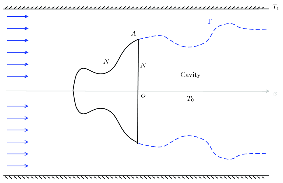
The second purpose of this paper is to establish the well-posedness theory of the jet flows of inviscid, incompressible fluid with general vorticity issuing from a semi-infinitely long nozzle for symmetric case (see Figure 1). It’s a direct and important application of the mathematical theory of the free boundary problem (1.1).

Refer to caption — Figure 1. Incompressible jet flow

Before we proceed with the bulk of this paper, we would like to mention the previous results on the well-posedness of the free boundary problem for incompressible inviscid jet flows.

For the irrotational inviscid incompressible flow without surface tension, the existence of an axisymmetric jet flow [5], an asymmetric jet flow [3] and impinging jet flow [12, 14] has been established based on the fundamental work [2]. The main advantage for two-dimensional irrotational flow is that the stream function $\displaystyle\psi$ solves the linear elliptic equation with Bernoulli’s type free boundary. And then the conformal mapping and Green function approach for the linear elliptic equation work for the irrotational flow. Furthermore, for the simplified setting of constant vorticity, which corresponds to a constant vorticity strength $\displaystyle f(\psi)\equiv P_{0}$ in (1.1), the well-posedness of axially symmetric cavitational flow in [24], symmetric impinging jet flow in [13] and symmetric cavitational flow in an infinitely long nozzle in [16] were established, based on the regularity of the free boundary problem with Poisson equation $\displaystyle\Delta\psi=P_{0}$ . The assumption of an inviscid incompressible jet with non-zero constant vorticity provides us with the simplest case of a flow that is not irrotational and is attractive for its analytical tractability. However, the simplicity setting is not a mere mathematical convenience, as it is also physical relevant. Indeed, the vorticity remains invariant along the each streamline for inviscid fluid, therefore the fluid possesses constant vorticity as long as we impose the constant vorticity in the upstream.

Generations of scientists working in fluid dynamics has recognized the importance of the vorticity. It has provided a powerful qualitative description for many of the important phenomena of fluid mechanics. From the mathematical point of view, the strong nonlinearity of the equations of vortex motion has made the analysis difficult.

In the present paper, to establish the well-posedness of the incompressible jet issuing from a semi-infinitely long nozzle with general vorticity, we will impose the vorticity in the inlet of the nozzle, and then the vorticity strength function $\displaystyle f(\psi)$ is determined uniquely along the streamlines. To realize this idea, one of the key points is to show the well-posedness of the streamlines. A free boundary problem with semilinear nonhomogeneous elliptic equation as (1.1) is formulated. An associated variational problem is shown to possess a minimizer, which yields a solution of semilinear free boundary problem.

2. Regularity and non-degeneracy of the solutions

To investigate the free boundary of the semilinear elliptic equation (1.1), based on the works [2, 6, 24] by Alt, Caffarelli and Friedman, we study the variational problem in this section, and establish the non-degeneracy lemma and the regularity of the solution.

2.1. The variational problem

Let $\displaystyle\Omega\subset\mathbb{R}^{2}$ be a bounded and connected open domain and $\displaystyle\partial\Omega$ is a locally Lipschitz graph, $\displaystyle I_{E}$ is the characteristic function of a set $\displaystyle E\subset\mathbb{R}^{2}$ and $\displaystyle f(t)\in C^{1,\beta}((-\infty,+\infty))$ , which satisfies that

\text{$\displaystyle 0\leq f(t)\leq\Lambda$ for any $\displaystyle t\leq 0$ and $\displaystyle-\Lambda\leq f^{\prime}(t)\leq 0$ for any $\displaystyle t\in\mathbb{R}$},

(2.1)

where $\displaystyle\Lambda\geq 0$ is a constant. Denote

F(t)=-2\int_{0}^{t}f(s)ds.

It is easy to check that

F(0)=0,\ -2\Lambda\leq F^{\prime}(t)\leq 0\ \text{for any $\displaystyle t\leq 0$ and}\ 0\leq F^{\prime\prime}(t)\leq 2\Lambda\ \text{for any $\displaystyle t\in\mathbb{R}$}.

(2.2)

Define a function $\displaystyle\Psi\in C^{0}(\bar{\Omega})\cap C^{2,\alpha}(\Omega)$ and $\displaystyle\Psi$ satisfies

\Delta\Psi+f(\Psi)\leq 0\ \ \text{in $\displaystyle\Omega$ and $\displaystyle\Psi>0$ in $\displaystyle\Omega$}.

(2.3)

Consider an energy functional

J(\psi)=\int_{\Omega}\left(|\nabla\psi|^{2}+F(\psi)+\lambda^{2}(X)I_{\{\psi>0\}}\right)dX,

and an admissible set

K=\{\phi\in H^{1}(\Omega)\mid~\phi\leq\Psi\ \text{a.e. in $\displaystyle\Omega$},~~\phi=\Psi_{0}\ \text{on}~S\},

where $\displaystyle S$ is a given subset of $\displaystyle\partial\Omega$ with $\displaystyle\mathcal{H}^{1}(S)>0$ , $\displaystyle\Psi_{0}\in H^{1}(\Omega)$ and $\displaystyle 0\leq\Psi_{0}\leq\Psi$ a.e. on $\displaystyle S$ , $\displaystyle\lambda(X)\in C^{0,\beta}(\bar{\Omega})$ and satisfies

0<\lambda_{1}\leq\lambda(X)\leq\lambda_{2}<+\infty\ \ \text{for any $\displaystyle X\in\bar{\Omega}$}.

(2.4)

The variational problem $\displaystyle(P)$ : Find a $\displaystyle\psi\in K$ , such that

J(\psi)=\min_{\phi\in K}J(\phi).

Remark 2.1.

For the special case $\displaystyle F(t)\equiv 0$ , the variational problem have been studied by Alt and Caffarelli in [2]. They established the Lipschitz continuity and non-degeneracy of the minimizer $\displaystyle\psi$ , and obtained the regularity of the free boundary. Moreover, Friedman in [24] investigated the variational problem for $\displaystyle F(t)=-2P(x,y)t$ with $\displaystyle P(x,y)\geq 0$ and $\displaystyle P(x,y)\in C^{0,1}(\bar{\Omega})$ , and established the regularity of the free boundary.

As the first step, the existence of the minimizer $\displaystyle\psi$ to the variational problem $\displaystyle(P)$ can be obtained by using the similar arguments in Lemma 1.3 in [2], we omit it here.

2.2. Lipschitz continuity of the minimizer

In this subsection, we will obtain the Lipschitz continuity of the minimizer $\displaystyle\psi$ .

We first focus on the Hölder continuity of the minimizer $\displaystyle\psi$ in $\displaystyle\Omega$ , and show that the minimizer $\displaystyle\psi$ satisfies the semilinear elliptic equation in $\displaystyle\Omega\cap\{\psi>0\}$ .

Lemma 2.1.

(1) $\displaystyle\psi\in C^{\alpha}(\Omega)$ for some $\displaystyle\alpha\in(0,1)$ and $\displaystyle\psi\geq 0$ in $\displaystyle\Omega$ .
(2) $\displaystyle\psi$ satisfies that

\displaystyle\Delta\psi+f(\psi)\geq 0

\displaystyle\Omega

(2.5)

in the weak sense and

\displaystyle\Delta\psi+f(\psi)=0

\displaystyle\Omega\cap\{\psi>0\}

(2.6)

Furthermore, $\displaystyle\psi\in C^{2,\alpha}(D)$ for any compact subset $\displaystyle D$ of $\displaystyle\Omega\cap\{\psi>0\}$ .

Proof.

(1) Let $\displaystyle B_{r}\subset\Omega$ and define a function $\displaystyle\phi$ as follows

\Delta\phi+f(\phi)=0\ \ \ \text{in}~~B_{r},\ \ \text{and}\ \ \ \phi=\psi\ \ \text{outside}\ \ B_{r}.

The maximum principle gives that $\displaystyle\phi\leq\Psi$ in $\displaystyle\Omega$ , and thus $\displaystyle\phi\in K$ . Then we have

\begin{array}[]{rl}0\leq&J(\phi)-J(\psi)\\ =&\int_{B_{r}}-|\nabla(\phi-\psi)|^{2}+2\nabla(\phi-\psi)\cdot\nabla\phi+F(\phi)-F(\psi)dX\\ &+\int_{B_{r}}\lambda^{2}(X)(I_{\{\phi>0\}}-I_{\{\psi>0\}})dX\\ \leq&\int_{B_{r}}-|\nabla(\phi-\psi)|^{2}dX+\lambda_{2}^{2}\int_{B_{r}}I_{\{\phi>0\}}dX,\end{array}

(2.7)

which implies that

\begin{array}[]{rl}\int_{B_{r}}|\nabla(\phi-\psi)|^{2}dX\leq\lambda_{2}^{2}\int_{B_{r}}I_{\{\phi>0\}}dX\leq\lambda_{2}^{2}\pi r^{2}.\end{array}

(2.8)

With the aid of gradient $\displaystyle L^{2}$ -estimate in (2.8), we can now use the method of Morrey in Theorem 5.3.6 in [28] to deduce the Hölder continuity of the minimizer.

Set $\displaystyle\psi^{\varepsilon}=\psi-\varepsilon\min\{\psi,0\}$ for any $\displaystyle\varepsilon\in(0,1)$ . It is clear that $\displaystyle\psi^{\varepsilon}\in K$ and $\displaystyle\psi^{\varepsilon}\geq\psi$ in $\displaystyle\Omega$ . Furthermore, $\displaystyle\psi>0$ if and only if $\displaystyle\psi^{\varepsilon}>0$ in $\displaystyle\Omega$ , and one has

\begin{array}[]{rl}0\leq&J(\psi^{\varepsilon})-J(\psi)\\ \leq&\int_{\Omega}((1-\varepsilon)^{2}-1)|\nabla\min\{\psi,0\}|^{2}-\varepsilon F^{\prime}((1-\varepsilon)\min\{\psi,0\})\min\{\psi,0\}dX.\end{array}

(2.9)

Since $\displaystyle F^{\prime}(t)\leq 0$ for any $\displaystyle t\leq 0$ in (2.2), it follows from (2.9) that

\int_{\Omega}|\nabla\min\{\psi,0\}|^{2}dX\leq 0,

which implies that

\text{$\displaystyle\psi(x,y)\geq 0$ in $\displaystyle\Omega$}.

(2) For any $\displaystyle\xi\in C_{0}^{\infty}(\Omega)$ with $\displaystyle\xi\geq 0$ in $\displaystyle\Omega$ , it follows from the statement (1) that $\displaystyle\psi-\varepsilon\xi\in K$ and $\displaystyle\{\psi-\varepsilon\xi>0\}\subset\{\psi>0\}$ for any $\displaystyle\varepsilon>0$ , then we have

\begin{array}[]{rl}0\leq&\lim_{\varepsilon\rightarrow 0}\left(\frac{1}{\varepsilon}\int_{\Omega}|\nabla\psi-\varepsilon\nabla\xi|^{2}-|\nabla\psi|^{2}+F(\psi-\varepsilon\xi)-F(\psi)dX\right)\\ =&-\int_{\Omega}2\nabla\psi\cdot\nabla\xi+F^{\prime}(\psi)\xi dX,\end{array}

which gives (2.5).

By virtue of the continuity of $\displaystyle\psi$ , we have that $\displaystyle\Omega\cap\{\psi>0\}$ is open. For any $\displaystyle\xi\in C_{0}^{\infty}(\Omega\cap\{\psi>0\})$ , it is easy to check that $\displaystyle\psi(x,y)-\varepsilon\xi(x,y)\leq\Psi(x,y)$ in $\displaystyle\Omega$ and $\displaystyle\{\psi-\varepsilon\xi>0\}\subset\{\psi>0\}$ for small $\displaystyle|\varepsilon|>0$ . Obviously, $\displaystyle\psi-\varepsilon\xi\in K$ and we have

\begin{array}[]{rl}0\leq-\varepsilon\int_{\Omega}2\nabla\psi\cdot\nabla\xi+F^{\prime}(\psi-\varepsilon\xi)\xi dX+o(\varepsilon),\end{array}

which implies that

0=\int_{\Omega}2\nabla\psi\cdot\nabla\xi+F^{\prime}(\psi-\varepsilon\xi)\xi dX\ \ \ \text{for any $\displaystyle\varepsilon$}.

(2.10)

Taking $\displaystyle\varepsilon\rightarrow 0$ in (2.10) yields (2.6).

It follows from the Schauder interior estimate in [26] that $\displaystyle\psi\in C^{2,\alpha}(D)$ for any compact subset $\displaystyle D$ of $\displaystyle\Omega\cap\{\psi>0\}$ .

∎

Denote

\Gamma=\Omega\cap\partial\{\psi>0\}\ \ \text{ the free boundary of $\displaystyle\psi$}.

The dynamic boundary condition on the free boundary $\displaystyle\Gamma$ can be verified in the following.

Proposition 2.2.

If $\displaystyle\lambda(X)\in C^{1,\beta}(\bar{\Omega})$ , for any minimizer $\displaystyle\psi$ , we have

\lim_{\varepsilon\downarrow 0}\int_{\Omega\cap\partial\{\psi>\varepsilon\}}\left(|\nabla\psi|^{2}-\lambda^{2}(X)-F(\psi)\right)\eta\cdot\nu_{\varepsilon}dS=0,

(2.11)

for any 2-vector $\displaystyle\eta\in\left(C_{0}^{1}(\Omega)\right)^{2}$ , where $\displaystyle\nu_{\varepsilon}$ is the outer normal vector to $\displaystyle\Omega\cap\partial\{\psi>\varepsilon\}$ with $\displaystyle\varepsilon>0$ . Similarly, if a segment $\displaystyle l\subset\partial\Omega\cap\partial\{\psi>0\}$ is $\displaystyle C^{1,\alpha}$ and $\displaystyle\psi=0$ on $\displaystyle l$ , we have

|\nabla\psi|\geq\lambda(X)\ \ \text{on $\displaystyle l$}.

(2.12)

Proof.

We define a diffeomorphism

Y=\xi_{\delta}(X):\Omega\rightarrow\Omega

by $\displaystyle\xi_{\delta}(X)=X+\delta\eta(X)$ for any $\displaystyle\eta(X)\in\left(C_{0}^{1}(\Omega)\right)^{2}$ , where $\displaystyle\delta$ is a real number and $\displaystyle|\delta|>0$ is suitable small.

Denote

\text{$\displaystyle\psi_{\delta}(\xi_{\delta}(X))=\psi(X)$}.

It’s easy to verify that $\displaystyle\psi_{\delta}\in K$ and

(D\xi_{\delta}(X))^{-1}=(E+\delta\nabla\cdot\eta E-\delta D\eta)(\text{det}D\xi_{\delta})^{-1}\quad\text{and}\quad\text{det}D\xi_{\delta}=1+\delta\nabla\cdot\eta+o(\delta),

where $\displaystyle E$ is the identity matrix. Then we have

\begin{array}[]{rl}0\leq&\int_{\Omega}\left(|\nabla\psi_{\delta}|^{2}+F(\psi_{\delta})+\lambda^{2}I_{\{\psi_{\delta}>0\}}\right)dY-\int_{\Omega}\left(|\nabla\psi|^{2}+F(\psi)+\lambda^{2}I_{\{\psi>0\}}\right)dX\\ =&\int_{\Omega}\left(|\nabla\psi(D\xi_{\delta})^{-1}|^{2}+F(\psi)+\lambda^{2}(\xi_{\delta}(X))I_{\{\psi>0\}}\right)\text{det}D\xi_{\delta}dX\\ &-\int_{\Omega}\left(|\nabla\psi|^{2}+F(\psi)+\lambda^{2}I_{\{\psi>0\}}\right)dX\\ =&\delta\int_{\Omega\cap\{\psi>0\}}\left((|\nabla\psi|^{2}+F(\psi)+\lambda^{2})\nabla\cdot\eta-2\nabla\psi\cdot D\eta\cdot\nabla\psi+\nabla\lambda^{2}\cdot\eta\right)dX+o(\delta).\end{array}

(2.13)

Due to the arbitrariness of $\displaystyle\delta$ , the linear term of (2.13) in $\displaystyle\delta$ has to vanish, and this gives that

\begin{array}[]{rl}0=&\int_{\Omega\cap\{\psi>0\}}\left((|\nabla\psi|^{2}+F(\psi)+\lambda^{2})\nabla\cdot\eta-2\nabla\psi\cdot D\eta\cdot\nabla\psi+\nabla\lambda^{2}\cdot\eta\right)dX\\ =&\int_{\Omega\cap\{\psi>0\}}\nabla\cdot\left((|\nabla\psi|^{2}+\lambda^{2}+F(\psi))\eta-2(\eta\cdot\nabla\psi)\nabla\psi\right)dX\\ =&\lim_{\varepsilon\downarrow 0}\int_{\Omega\cap\partial\{\psi>\varepsilon\}}\left((|\nabla\psi|^{2}+\lambda^{2}+F(\psi))\eta-2(\eta\cdot\nabla\psi)\nabla\psi\right)\cdot\nu_{\varepsilon}dS\\ =&\lim_{\varepsilon\downarrow 0}\int_{\Omega\cap\partial\{\psi>\varepsilon\}}\left(\lambda^{2}(X)-|\nabla\psi|^{2}+F(\psi)\right)\eta\cdot\nu_{\varepsilon}dS.\end{array}

(2.14)

Hence, we obtain the conclusion (2.11). To prove (2.12), define $\displaystyle\xi_{\delta}(X)=X+\delta\eta(X)$ for any $\displaystyle\eta(X)\in\left(C^{1}(\Omega\cap\partial\{\psi>0\})\right)^{2}$ with $\displaystyle\eta=0$ on $\displaystyle(\Omega\cap\partial\{\psi>0\})\setminus l$ and $\displaystyle\eta\cdot\nu\leq 0$ on $\displaystyle l$ , where $\displaystyle\delta>0$ is suitable small and $\displaystyle\nu$ is the outer normal vector of $\displaystyle l$ .

Along the similar arguments in (2.13) and (2.14), we have

\begin{array}[]{rl}0\leq&\int_{\Omega\cap\{\psi>0\}}\left((|\nabla\psi|^{2}+F(\psi)+\lambda^{2})\nabla\cdot\eta-2\nabla\psi\cdot D\eta\cdot\nabla\psi+\nabla\lambda^{2}(X)\cdot\eta\right)dX\\ =&\int_{\Omega\cap\{\psi>0\}}\nabla\cdot\left((|\nabla\psi|^{2}+\lambda^{2}+F(\psi))\eta-2(\eta\cdot\nabla\psi)\nabla\psi\right)dX\\ =&\int_{l}\left(\lambda^{2}(X)-|\nabla\psi|^{2}+F(\psi)\right)\eta\cdot\nu dS.\end{array}

(2.15)

Since $\displaystyle l\in C^{1,\alpha}$ , $\displaystyle\psi$ is also $\displaystyle C^{1}$ up to $\displaystyle l$ . Therefore, we complete the proof of (2.12) by using (2.15).

∎

Remark 2.2.

Proposition 2.2 implies that if the free boundary $\displaystyle\Gamma$ is $\displaystyle C^{1}$ and $\displaystyle\psi$ is $\displaystyle C^{1}$ in $\displaystyle\{\psi>0\}$ uniformly up to the free boundary, then

|\nabla\psi(X)|=\lambda(X)\ \ \text{on the free boundary $\displaystyle\Gamma$}.

Next, we will give the estimate for the Lipschitz norm for $\displaystyle\psi$ near the free boundary, this is the principal part in establishing the Lipschitz continuity of the minimizer $\displaystyle\psi$ . Denote

\Omega_{+}=\Omega\cap\{\psi>0\}\ \ \text{and}\ \ \Omega_{0}=\Omega\cap\{\psi=0\}.

Lemma 2.3.

Suppose $\displaystyle X_{0}=(x_{0},y_{0})\in\Omega$ with $\displaystyle d(X_{0})<\frac{1}{2}\min\{\text{dist}(X_{0},\partial\Omega),1\}$ , where $\displaystyle d(X_{0})=\text{dist}(X_{0},\Omega_{0})$ . Then there exists a positive constant $\displaystyle C=C(\Lambda)$ depending only on $\displaystyle\Lambda$ , such that

\psi(X_{0})\leq C(\lambda_{2}+\Lambda)d(X_{0}),

where $\displaystyle\Lambda$ is defined in (2.1).

Proof.

We assume that

\psi(X_{0})>Md(X_{0})>0,

(2.16)

and derive an upper bound on $\displaystyle M$ . Denote $\displaystyle d=d(X_{0})$ for simplicity. By scaling $\displaystyle\psi_{d}(X)=\frac{\psi(X_{0}+d(X-X_{0}))}{d}$ and $\displaystyle\lambda_{d}(X)=\lambda(X_{0}+d(X-X_{0}))$ with $\displaystyle X\in B_{1}(X_{0})$ , we have

\displaystyle\Delta\psi_{d}+df(d\psi_{d})=0\

\displaystyle B_{1}(X_{0})

On the other hand, it is easy to check that

|df(d\psi_{d})|\leq d|f(0)|+d^{2}\max_{\xi\geq 0}|f^{\prime}(\xi)|\psi_{d}\leq d\Lambda+d^{2}\Lambda\psi_{d}.

Thanks to Harnack’s inequality in [31] and (2.16), we have

\inf_{B_{\frac{3}{4}}(X_{0})}\psi_{d}\geq cM-Cd\Lambda\geq cM-C\Lambda,

(2.17)

where the constants $\displaystyle c$ and $\displaystyle C$ depend on $\displaystyle\Lambda$ .

Let $\displaystyle Y$ be a point in $\displaystyle\partial B_{1}(X_{0})\cap\{\psi_{d}=0\}$ . Define a function $\displaystyle\phi$ as follows

\Delta\phi+df(d\phi)=0\ \ \ \text{in}~~B_{1}(Y),\ \ \text{and}\ \ \ \phi=\psi_{d}\ \ \text{on}\ \ \partial B_{1}(Y).

Since $\displaystyle\psi_{d}$ is a minimizer, by virtue of the convexity of $\displaystyle F(t)$ , one has

\begin{array}[]{rl}0\leq&\int_{B_{1}(Y)}|\nabla\phi|^{2}-|\nabla\psi_{d}|^{2}+F(d\phi)-F(d\psi_{d})+\lambda_{d}^{2}(I_{\{\phi>0\}}-I_{\{\psi_{d}>0\}})dX\\ \leq&\int_{B_{1}(Y)}-|\nabla(\phi-\psi_{d})|^{2}+2\nabla(\phi-\psi_{d})\cdot\nabla\phi dX\\ &+\int_{B_{1}(Y)}dF^{\prime}(d\phi)(\phi-\psi_{d})+\lambda_{d}^{2}I_{\{\psi_{d}=0\}}dX\\ \leq&-\int_{B_{1}(Y)}|\nabla(\phi-\psi_{d})|^{2}dX+\lambda_{2}^{2}\int_{B_{1}(Y)}I_{\{\psi_{d}=0\}}dX,\end{array}

and thus

\begin{array}[]{rl}\int_{B_{1}(Y)}|\nabla(\phi-\psi_{d})|^{2}dX\leq\lambda_{2}^{2}\int_{B_{1}(Y)}I_{\{\psi_{d}=0\}}dX.\end{array}

(2.18)

It follows from the statement (2) in Lemma 2.1 that $\displaystyle\Delta\psi_{d}+df(d\psi_{d})\geq 0$ in $\displaystyle B_{1}(Y)$ , and the maximum principle gives that

\phi\geq\psi_{d}\ \ \text{in}\ \ B_{1}(Y).

(2.19)

Then it follows from (2.17) and (2.19) that

\phi(X)\geq\psi_{d}(X)\geq cM-C\Lambda>0\ \ \text{in}\ \ B_{\frac{3}{4}}(X_{0})\cap B_{1}(Y).

Using Harnack’s inequality in [31] again, we have

\phi(X)\geq cM-C\Lambda=C_{0}>0\ \ \text{in}\ \ B_{\frac{1}{2}}(Y).

(2.20)

We take $\displaystyle Y=0$ for simplicity and introduce a function

\varphi(X)=C_{0}\left(e^{-\beta|X|^{2}}-e^{-\beta}\right).

Then a direct computation gives that

\Delta\varphi+df(d\varphi)\geq C_{0}e^{-\beta|X|^{2}}(4\beta(\beta|X|^{2}-1)-d^{2}\Lambda)+C_{0}d^{2}\Lambda e^{-\beta}+df(0)>0,

for $\displaystyle\frac{1}{2}<|X|<1$ , and sufficiently large $\displaystyle\beta>0$ . This gives that

\Delta(\varphi-\phi)+df(d\varphi)-df(d\phi)>0\ \ \text{in}\ \ B_{1}(0)\setminus B_{\frac{1}{2}}(0),

provided that $\displaystyle\beta$ is sufficiently large. It follows from the maximum principle that

\phi(X)>\varphi(X)=C_{0}\left(e^{-\beta|X|^{2}}-e^{-\beta}\right)\geq cC_{0}(1-|X|)\ \ \text{in}\ \ B_{1}(0)\setminus B_{\frac{1}{2}}(0),

which implies that

\phi(X)>(cM-C\Lambda)(1-|X|)\ \ \text{in}\ \ B_{1}(0)\setminus B_{\frac{1}{2}}(0).

This together with (2.20) gives that

\phi(X)\geq(cM-C\Lambda)(1-|X|)\ \ \text{in}\ \ B_{1}(0).

(2.21)

With the aid of (2.18) and (2.21), it follows from the similar arguments in Lemma 3.2 in [2] and Lemma 2.2 in [6] that

(cM-C\Lambda)^{2}\leq C\max_{X\in\Omega}\lambda^{2}(X)=C\lambda_{2}^{2},

that is

M\leq C(\lambda_{2}+\Lambda),

where the constant $\displaystyle C=C(\Lambda)$ depends only on $\displaystyle\Lambda$ .

∎

With the aid of Lemma 2.3, we will obtain the Lipschitz continuity of $\displaystyle\psi$ , which plays an essential part for constructing a Radon measure. To obtain the Lipschitz continuity, we should use the method of Harnack’s inequality in [31].

Theorem 2.4.

(1). The minimizer $\displaystyle\psi$ is Lipschitz continuous in $\displaystyle\Omega$ , namely, $\displaystyle\psi\in C^{0,1}(\Omega)$ .
(2). For any compact subset $\displaystyle D$ of $\displaystyle\Omega$ which containing a free boundary point, the Lipschitz coefficient of $\displaystyle\psi$ in $\displaystyle D$ is estimated by $\displaystyle C(\lambda_{2}+\Lambda)$ , and the constant $\displaystyle C$ depends only on $\displaystyle\Lambda$ , $\displaystyle D$ and $\displaystyle\Omega$ .

Proof.

(1). Suppose that $\displaystyle d(X_{0})<\frac{1}{3}\min\{\text{dist}(X_{0},\partial\Omega),1\}$ , where $\displaystyle d(X_{0})=\text{dist}(X_{0},\Omega_{0})$ . Set

\tilde{\psi}(\tilde{X})=\frac{\psi(X_{0}+d(X_{0})\tilde{X})}{d(X_{0})}.

By virtue of Lemma 2.3, one has

\tilde{\psi}(\tilde{X})\leq C(\lambda_{2}+\Lambda)\ \ \text{in}\ \ B_{1}(0),

where the constant $\displaystyle C=C(\Lambda)$ depends only on $\displaystyle\Lambda$ .

Since $\displaystyle\Delta\tilde{\psi}+d(X_{0})f(d(X_{0})\tilde{\psi})=0$ in $\displaystyle B_{1}(0)$ , it follows from the elliptic estimate for $\displaystyle\tilde{\psi}$ that

\begin{array}[]{rl}|\nabla\tilde{\psi}(0)|\leq&C(\|\tilde{\psi}\|_{C^{0}(B_{1}(0))}+\|f(d(X_{0})\tilde{\psi})\|_{L^{\infty}(B_{1}(0))}d(X_{0}))\\ \leq&C(1+d^{2}(X_{0})|f(0)|+d^{2}(X_{0})\Lambda)\|\tilde{\psi}\|_{C^{0}(B_{1}(0))}\\ \leq&C(\lambda_{2}+\Lambda),\end{array}

which implies that

|\nabla\psi(X_{0})|=|\nabla\tilde{\psi}(0)|\leq C(\lambda_{2}+\Lambda).

Thus, for any compact subset $\displaystyle D$ of $\displaystyle\Omega$ , $\displaystyle|\nabla\psi(X)|$ is bounded in $\displaystyle D\cap\{\psi>0\}\cap U$ , where $\displaystyle U$ is a small neighborhood of the free boundary. It follows from Lemma 2.1 that $\displaystyle\psi\in C^{2,\alpha}$ in $\displaystyle\Omega\cap\{\psi>0\}$ , this together with $\displaystyle\nabla\psi=0$ a.e. in $\displaystyle\Omega\cap\{\psi=0\}$ gives that $\displaystyle\psi\in C^{0,1}(\Omega)$ .

(2). Consider any connected domains $\displaystyle D\subset\subset G\subset\subset\Omega$ and $\displaystyle D$ contains at least one free boundary point. Let $\displaystyle r_{0}=\frac{1}{5}\min\{\text{dist}(G,\partial\Omega),1\}$ and $\displaystyle X\in G\cap\Omega_{+}$ . Since $\displaystyle D$ contains some free boundary points, and we have that $\displaystyle G$ is not contained in $\displaystyle\Omega_{+}$ , then we can find some finite points $\displaystyle X_{1},X_{2},...,X_{m}$ in $\displaystyle G$ ( $\displaystyle m$ depends only on $\displaystyle G$ and $\displaystyle\Omega$ ), such that

X_{0}=X,\ \ X_{k}\in B_{r_{0}}(X_{k-1})\ \text{for}\ \ k=1,...,m,

and

B_{2r_{0}}(X_{k})\subset\Omega_{+}\ \text{for}\ \ k=1,...,m-1,\text{and $\displaystyle B_{2r_{0}}(X_{m})$ is not contained in $\displaystyle\Omega_{+}$}.

It follows from Lemma 2.1 and Lemma 2.3 that

\psi(X_{m})\leq C(\lambda_{2}+\Lambda)r_{0}\ \ \text{and}\ \ \Delta\psi+f(\psi)=0\ \ \text{in}\ \ B_{2r_{0}}(X_{k})\ \text{for}\ \ k=1,...,m-1.

By virtue of Harnack’s inequality in [31], we have

\psi(X_{k-1})\leq C\psi(X_{k})+C\Lambda r_{0}\ \text{for}\ \ k=1,...,m-1,

and

\psi(X_{m-1})\leq C\inf_{X\in B_{2r_{0}}(X_{m-1})}\psi(X)+C\Lambda r_{0}\leq C\psi(X_{m})+C\Lambda r_{0}.

Inductively, we have

\psi(X)=\psi(X_{0})\leq C(\lambda_{2}+\Lambda)\ \ \text{for all $\displaystyle X\in G$}.

(2.22)

For any $\displaystyle X\in D\cap\Omega_{+}$ and $\displaystyle d(X)=\text{dist}(X,\Omega_{0})$ . We consider the following two cases.

Case 1. $\displaystyle d(X)\geq\frac{1}{2}\min\{dist(D,\partial G),1\}$ , by using elliptic estimate and (2.22), one has

|\nabla\psi(X)|\leq C\left(\sup_{G}\psi+\sup_{G}|f(\psi)|\right)\leq C(\lambda_{2}+\Lambda),

where $\displaystyle C$ is a constant depending only on $\displaystyle\Lambda$ , $\displaystyle D,G$ and $\displaystyle\Omega$ .

Case 2. $\displaystyle d(X)<\frac{1}{2}\min\{dist(D,\partial G),1\}$ , it follows from Lemma 2.3 that

|\nabla\psi(X)|\leq C(\lambda_{2}+\Lambda),

where $\displaystyle C$ is a constant depending only on $\displaystyle\Lambda$ .

Hence, we complete the proof of Theorem 2.4.

∎

2.3. Non-degeneracy of the minimizer

As a consequence of Theorem 2.4, we will obtain the non-degeneracy lemma of the minimizer $\displaystyle\psi$ in this subsection.

Lemma 2.5.

Let $\displaystyle\psi$ be a minimizer, for any compact subset $\displaystyle D$ of $\displaystyle\Omega$ , there exists a positive constant $\displaystyle C^{*}$ (depending only on $\displaystyle\Lambda,D$ and $\displaystyle\Omega$ ), such that for any disc $\displaystyle B_{r}(X_{0})\subset D$ ,

\frac{1}{r}\fint_{\partial B_{r}(X_{0})}\psi dS\geq C^{*}(\lambda_{2}+\Lambda)

(2.23)

implies that

\psi(x,y)>0\ \ ~~~~\text{in}\ ~~B_{r}(X_{0}).

Proof.

Suppose that there exists a free boundary point $\displaystyle X^{\prime}\in B_{r}(X_{0})\cap\Omega_{0}$ . It follows from Theorem 2.4 that $\displaystyle|\nabla\psi|\leq C(\lambda_{2}+\Lambda)$ , where $\displaystyle C$ is a constant depending only on $\displaystyle\Lambda,D$ and $\displaystyle\Omega$ . Then we have

\psi(X)=\psi(X)-\psi(X^{\prime})\leq C(\lambda_{2}+\Lambda)r\ \ \text{in}\ \ \overline{B}_{r},

which contradicts to (2.23), provided that $\displaystyle C^{*}$ is sufficiently large. ∎

The non-degeneracy lemma will be stated in the following.

Lemma 2.6.

For any $\displaystyle\kappa\in(0,1)$ , there exists a positive constant $\displaystyle c^{*}_{\kappa}=c^{*}(\kappa)$ , such that for any disc $\displaystyle B_{r}(X_{0})\subset\Omega$ with $\displaystyle r<\frac{1}{\Lambda}\min\{c_{\kappa}^{*}\lambda_{1},1\}$ ,

\frac{1}{r}\fint_{\partial B_{r}(X_{0})}\psi dS\leq c_{\kappa}^{*}\lambda_{1}

(2.24)

implies that

\psi(x,y)\equiv 0~~~~\text{in}~~B_{\kappa r}(X_{0}).

Proof.

Without loss of generality, we assume that $\displaystyle X_{0}=0$ . Set $\displaystyle\psi_{r}(X)=\frac{\psi(rX)}{r}$ and $\displaystyle\lambda_{r}(X)=\lambda(rX)$ , we have

\Delta\psi_{r}+rf(r\psi_{r})=0\ \ \ \text{in}~~\Omega_{r}\cap\{\psi_{r}>0\},

where $\displaystyle\Omega_{r}=\{X\mid rX\in\Omega\}$ . Denote

\varepsilon=\sup_{X\in B_{\sqrt{\kappa}}(0)}\psi_{r}(X).

Since $\displaystyle\Delta\psi_{r}\geq-rf(r\psi_{r})\geq-rf(0)\geq-\Lambda r$ in $\displaystyle\Omega$ , it follows from the maximum principle that

\psi_{r}(X)\leq\Lambda r\frac{1-|X|^{2}}{4}+\frac{1-|X|^{2}}{2\pi}\int_{\partial B_{1}(0)}\frac{\psi_{r}(Y)}{|X-Y|^{2}}dS_{Y}

for any $\displaystyle X\in B_{\sqrt{\kappa}}(0)$ , which implies that

\varepsilon=\sup_{X\in B_{\sqrt{\kappa}}(0)}\psi_{r}(X)\leq\Lambda r+C(\kappa)\fint_{\partial B_{1}(0)}\psi_{r}(Y)dS_{Y}.

(2.25)

Define a function $\displaystyle\phi$ solving the following problem

\left\{\begin{array}[]{ll}&\Delta\phi+rf(r\phi)=0~~~~\text{in}\ \ \ B_{\sqrt{\kappa}}(0)\setminus B_{\kappa}(0),\\ &\phi=0~~~~\text{in}\ \ \ B_{\kappa}(0),\ \ \ \ \ \phi=\varepsilon~~~~\text{outside}\ \ \ B_{\sqrt{\kappa}}(0).\end{array}\right.

It is easy to check that

\begin{array}[]{rl}0\leq&\int_{B_{\sqrt{\kappa}}(0)}|\nabla\min\{\psi_{r},\phi\}|^{2}+F(r\min\{\psi_{r},\phi\})+\lambda_{r}^{2}I_{\{\min\{\psi_{r},\phi\}>0\}}dX\\ &-\int_{B_{\sqrt{\kappa}}(0)}|\nabla\psi_{r}|^{2}+F(r\psi_{r})+\lambda_{r}^{2}I_{\{\psi_{r}>0\}}dX,\end{array}

which yields that

\begin{array}[]{rl}&\int_{B_{\kappa}(0)}|\nabla\psi_{r}|^{2}+F(r\psi_{r})+\lambda_{r}^{2}I_{\{\psi_{r}>0\}}dX\\ \leq&\int_{B_{\sqrt{\kappa}}(0)\setminus B_{\kappa}(0)}|\nabla\min\{\psi_{r},\phi\}|^{2}+F(r\min\{\psi_{r},\phi\})-|\nabla\psi_{r}|^{2}-F(r\psi_{r})dX\\ \leq&\int_{B_{\sqrt{\kappa}}(0)\setminus B_{\kappa}(0)}-|\nabla\min\{\phi-\psi_{r},0\}|^{2}+2\nabla\phi\cdot\nabla\min\{\phi-\psi_{r},0\}\\ &+rF^{\prime}(r\phi)\min\{\phi-\psi_{r},0\}dX\\ \leq&2\int_{\partial B_{\kappa}(0)}\min\{\phi-\psi_{r},0\}\frac{\partial\phi}{\partial\nu}dS,\end{array}

(2.26)

where $\displaystyle\nu$ is the outer normal vector, we have used the fact

\int_{B_{\sqrt{\kappa}}(0)\setminus B_{\kappa}(0)}I_{\{\min\{\psi_{r},\phi\}>0\}}-I_{\{\psi_{r}>0\}}dX\leq 0,

due to the fact $\displaystyle\{\min\{\psi_{r},\phi\}>0\}\subset\{\psi_{r}>0\}$ .

On the other hand, by virtue of the convexity of $\displaystyle F(t)$ , we have that

F(r\psi_{r})\geq F^{\prime}(0)r\psi_{r}\geq-2\Lambda r\psi_{r},

which gives that

\begin{array}[]{rl}&\int_{B_{\kappa}(0)}|\nabla\psi_{r}|^{2}-2\Lambda r\psi_{r}+\lambda_{r}^{2}I_{\{\psi_{r}>0\}}dX\leq\int_{B_{\kappa}(0)}|\nabla\psi_{r}|^{2}+F(r\psi_{r})+\lambda_{r}^{2}I_{\{\psi_{r}>0\}}dX.\end{array}

(2.27)

The standard elliptic estimates give that

\sup_{X\in\partial B_{\kappa}(0)}|\nabla\phi(X)|\leq C\left(\sup_{X\in B_{\sqrt{\kappa}}(0)}\phi(X)+r\|f(r\phi)\|_{L^{\infty}(B_{\sqrt{\kappa}}(0))}\right)\leq C(\Lambda,\kappa)(\varepsilon+\Lambda r).

(2.28)

Furthermore, with the aid of the trace theorem, it follows from (2.26) - (2.28) that

\begin{array}[]{rl}&\int_{B_{\kappa}(0)}|\nabla\psi_{r}|^{2}+\lambda_{r}^{2}I_{\{\psi_{r}>0\}}dX\\ \leq&2\int_{\partial B_{\kappa}(0)}\min\{\phi-\psi_{r},0\}\frac{\partial\phi}{\partial\nu}dS+2\int_{B_{\kappa}(0)}\Lambda r\psi_{r}dX\\ \leq&C(\Lambda,\kappa)\varepsilon_{0}\left(\int_{\partial B_{\kappa}(0)}\psi_{r}dS+\int_{B_{\kappa}(0)}\psi_{r}dX\right)\\ \leq&C(\Lambda,\kappa)\varepsilon_{0}\left(\int_{B_{\kappa}(0)}\psi_{r}I_{\{\psi_{r}>0\}}dX+C\int_{B_{\kappa}(0)}|\nabla\psi_{r}|I_{\{\psi_{r}>0\}}dX\right)\\ \leq&C(\Lambda,\kappa)\varepsilon_{0}\left(\frac{\varepsilon_{0}}{\lambda_{1}^{2}}\int_{B_{\kappa}(0)}I_{\{\psi_{r}>0\}}dX+\frac{C}{\lambda_{1}}\int_{B_{\kappa}(0)}|\nabla\psi_{r}|^{2}+\lambda_{r}^{2}I_{\{\psi_{r}>0\}}dX\right)\\ \leq&C(\Lambda,\kappa)\left(\frac{\varepsilon^{2}_{0}}{\lambda_{1}^{2}}+\frac{\varepsilon_{0}}{\lambda_{1}}\right)\int_{B_{\kappa}(0)}|\nabla\psi_{r}|^{2}+\lambda_{r}^{2}I_{\{\psi_{r}>0\}}dX,\end{array}

(2.29)

where $\displaystyle\varepsilon_{0}=\varepsilon+\Lambda r$ . By virtue of (2.24) and (2.25), one has

\frac{\varepsilon_{0}}{\lambda_{1}}=\frac{\varepsilon+\Lambda r}{\lambda_{1}}\leq C(\Lambda,\kappa)\left(\frac{1}{\lambda_{1}}\fint_{\partial B_{1}(0)}\psi_{r}dS+\frac{\Lambda r}{\lambda_{1}}\right)<C(\Lambda,\kappa)c_{\kappa}^{*}.

This implies that $\displaystyle\frac{\varepsilon_{0}}{\lambda_{1}}$ is small enough, provided that $\displaystyle c_{\kappa}^{*}$ is small enough. This together with (2.29) implies that

\int_{B_{\kappa}(0)}|\nabla\psi_{r}|^{2}+\lambda_{r}^{2}I_{\{\psi_{r}>0\}}dX=0,\ \

for sufficiently small $\displaystyle c_{\kappa}^{*}$ . This implies that $\displaystyle\psi=0$ in $\displaystyle B_{\kappa}(0)$ , if $\displaystyle c_{\kappa}^{*}$ is small enough.

∎

Remark 2.3.

It should be noted that Lemma 2.5 remains valid, provided that $\displaystyle B_{r}(X_{0})$ is not contained in $\displaystyle\Omega$ and $\displaystyle\psi=0$ on $\displaystyle B_{r}(X_{0})\cap\partial\Omega$ .

Finally, we give the density estimate of the free boundary point, which gives that $\displaystyle\mathcal{L}^{2}(D\cap\partial\{\psi>0\})=0$ for any compact subset $\displaystyle D$ of $\displaystyle\Omega$ .

Lemma 2.7.

Let $\displaystyle G$ be a compact subset of $\displaystyle\Omega$ , there exists a positive constant $\displaystyle c\in(0,1)$ , such that for any disc $\displaystyle B_{r}=B_{r}(X_{0})\subset G$ with $\displaystyle X_{0}\in\Gamma$ and small $\displaystyle r$ ,

c<\frac{\mathcal{L}^{2}(B_{r}\cap\{\psi>0\})}{\mathcal{L}^{2}(B_{r})}<1-c,

(2.30)

where $\displaystyle\mathcal{L}^{2}$ is the two-dimensional Lebesgue measure.

Proof.

Step 1. Without loss of generality, we assume that $\displaystyle X_{0}=0$ . It follows from Lemma 2.6 that there exists a point $\displaystyle Y\in\partial B_{r}$ , such that $\displaystyle\psi(Y)>cr$ . Set $\displaystyle\varphi(X)=\psi(X)+\frac{\Lambda|X|^{2}}{4}$ , one has

\Delta\varphi=\Delta\psi+\Lambda\geq f(0)-f(\psi)\geq 0\ \ \ \text{in $\displaystyle B_{r}$},

which implies that

\frac{\Lambda r}{2\kappa}+\frac{1}{\kappa r}\fint_{\partial B_{\kappa r}(Y)}\psi(Z)dS_{Z}\geq\frac{1}{\kappa r}\fint_{\partial B_{\kappa r}(Y)}\varphi(Z)dS_{Z}\geq\frac{\varphi(Y)}{\kappa r}\geq\frac{c}{\kappa},

for small $\displaystyle\kappa>0$ , that is

\frac{1}{\kappa r}\fint_{\partial B_{\kappa r}(Y)}\psi(Z)dS_{Z}\geq\frac{c-\Lambda r}{2\kappa}>\frac{c}{4\kappa}\ \ \text{if $\displaystyle r$ is small enough}.

By virtue of non-degeneracy Lemma 2.6, one has

\displaystyle\psi>0

\displaystyle B_{\kappa r}(Y)

this gives the left-hand side of (2.30).

Step 2. Define a function $\displaystyle\phi$ solving the following problem

\Delta\phi+f(\phi)=0~~~~\text{in}~~B_{r},\ \ \phi=\psi~~~~~~\text{outside}~~B_{r}.

The maximum principle gives that $\displaystyle\psi\leq\phi\leq\Psi$ in $\displaystyle B_{r}$ , and thus $\displaystyle\phi\in K$ , where $\displaystyle\Psi$ is defined in (2.3).

Then we have

\begin{array}[]{rl}0\leq J(\phi)-J(\psi)\leq\int_{B_{r}}-|\nabla(\phi-\psi)|^{2}dX+\lambda_{2}^{2}\int_{B_{r}}I_{\{\psi=0\}}dX,\end{array}

which together with Poincaré’s inequality and Hölder inequality implies that

\begin{array}[]{rl}\lambda_{2}^{2}\int_{B_{r}}I_{\{\psi=0\}}dX\geq&\int_{B_{r}}|\nabla(\phi-\psi)|^{2}dX\geq\frac{c}{r^{2}}\int_{B_{r}}|\phi-\psi|^{2}dX.\end{array}

(2.31)

For any point $\displaystyle Y\in B_{\kappa r}$ , since $\displaystyle\Delta\phi\leq M_{0}\Lambda-f(0)$ with $\displaystyle M_{0}=\sup_{X\in\Omega}\Psi(X)$ , one has

\begin{array}[]{rl}\phi(Y)\geq&\frac{r^{2}-|Y|^{2}}{2\pi r}\int_{\partial B_{r}}\frac{\psi}{|X-Y|^{2}}dS_{X}+(M_{0}\Lambda-f(0))\frac{|Y|^{2}-r^{2}}{4}\\ \geq&(1-C\kappa)\fint_{\partial B_{r}}\psi dS_{X}-Cr^{2}.\end{array}

(2.32)

It follows from (2.32), Lemma 2.3 and Lemma 2.6 that

\begin{array}[]{rl}\phi(Y)-\psi(Y)\geq&\phi(Y)-C\kappa r\\ \geq&(1-C\kappa)\fint_{\partial B_{r}}\psi dS_{X}-C\kappa r-Cr^{2}\\ \geq&c\lambda_{1}r,\end{array}

(2.33)

provided that $\displaystyle\kappa$ and $\displaystyle r$ are small.

Combining (2.31) and (2.33), we have

\begin{array}[]{rl}\lambda_{2}^{2}\int_{B_{r}}I_{\{\psi=0\}}dX\geq\frac{c}{r^{2}}\int_{B_{r}}|\phi-\psi|^{2}dX\geq\frac{c}{r^{2}}\int_{B_{\kappa r}}|\phi-\psi|^{2}dX\geq&c_{\kappa}\lambda_{1}^{2}r^{2},\end{array}

(2.34)

for small $\displaystyle r>0$ and small $\displaystyle\kappa>0$ . This gives the right-hand side of (2.30).

∎

3. Regularity of the free boundary

Based on the Lipschitz continuity and non-degeneracy lemma of the minimizer $\displaystyle\psi$ in Section 2, we will establish the regularity of the free boundary in this section.

3.1. Measure estimate of the free boundary

In this subsection, the main objective is to show that the set $\displaystyle\Omega\cap\{\psi>0\}$ is finite perimeter locally in $\displaystyle\Omega$ .

Set $\displaystyle\mu=\Delta\psi+f(\psi)$ and $\displaystyle\mu_{0}=\Delta\psi+f(\psi)I_{\{\psi>0\}}$ . First, we will show that $\displaystyle\mu_{0}$ is a Radon measure supported on the free boundary $\displaystyle\Gamma$ .

Lemma 3.1.

$\displaystyle\mu_{0}=\Delta\psi+f(\psi)I_{\{\psi>0\}}$ is a positive Radon measure with support in $\displaystyle\Omega\cap\partial\{\psi>0\}$ . Moreover, $\displaystyle\mu=\Delta\psi+f(\psi)$ is a Radon measure supported on $\displaystyle\Omega\cap\{\psi=0\}$ and its singular point is contained in the free boundary.

Proof.

For any $\displaystyle\xi\in C_{0}^{\infty}(\Omega)$ with $\displaystyle\xi\geq 0$ , denote $\displaystyle k(t)=\max\{\min\{2-t,1\},0\}$ for any $\displaystyle t>0$ . Then we have

\begin{array}[]{rl}\int_{\Omega}\nabla\psi\cdot\nabla(\xi k(t\psi))dX=&\int_{\Omega}\nabla\psi\cdot\nabla\xi dX+\int_{\Omega\cap\{\psi\geq\frac{1}{t}\}}\nabla\psi\cdot\nabla(\xi k(t\psi)-\xi)dX\\ =&\int_{\Omega}\nabla\psi\cdot\nabla\xi dX-\int_{\Omega\cap\{\psi>0\}}f(\psi)\xi dX\\ &+\int_{\Omega\cap\{\frac{1}{t}\leq\psi\leq\frac{2}{t}\}}(2-\psi t)f(\psi)\xi dX+\int_{\Omega\cap\{\psi\leq\frac{2}{t}\}}f(\psi)\xi dX\\ \geq&\int_{\Omega}\nabla\psi\cdot\nabla\xi dX-\int_{\Omega\cap\{\psi>0\}}f(\psi)\xi dX,\end{array}

(3.1)

for sufficiently large $\displaystyle t>0$ , where we have used the fact that $\displaystyle f(\psi)\geq\frac{f(0)}{2}\geq 0$ in $\displaystyle\Omega\cap\left\{\psi\leq\frac{2}{t}\right\}$ for large $\displaystyle t>0$ .

On the other hand, one has

\begin{array}[]{rl}\int_{\Omega}\nabla\psi\cdot\nabla(\xi k(t\psi))dX=&\int_{\Omega\cap\{\frac{1}{t}\leq\psi\leq\frac{2}{t}\}}(2-\psi t)\nabla\psi\cdot\nabla\xi-\xi t|\nabla\psi|^{2}dX\\ &+\int_{\Omega\cap\{0<\psi\leq\frac{1}{t}\}}\nabla\psi\cdot\nabla\xi dX\\ \leq&\int_{\Omega\cap\{0<\psi\leq\frac{2}{t}\}}|\nabla\psi||\nabla\xi|dX.\end{array}

(3.2)

It follows from (3.1) and (3.2) that

\begin{array}[]{rl}\int_{\Omega}\nabla\psi\cdot\nabla\xi dX-\int_{\Omega\cap\{\psi>0\}}f(\psi)\xi dX\leq\int_{\Omega\cap\{0<\psi\leq\frac{2}{t}\}}|\nabla\psi||\nabla\xi|dX.\end{array}

(3.3)

Taking $\displaystyle t\rightarrow+\infty$ in (3.3), we conclude that $\displaystyle\Delta\psi+f(\psi)I_{\{\psi>0\}}\geq 0$ in the sense of distributions. Consequently, there exists a positive Radon measure $\displaystyle\mu_{0}$ supported on $\displaystyle\Omega\cap\partial\{\psi>0\}$ , such that $\displaystyle\mu_{0}=\Delta\psi+f(\psi)I_{\{\psi>0\}}$ .

Recalling $\displaystyle f(0)\geq 0$ , there exists a positive Radon measure $\displaystyle\mu$ supported on $\displaystyle\Omega\cap\{\psi=0\}$ , such that $\displaystyle\mu=\mu_{0}+f(0)I_{\{\psi=0\}}=\Delta\psi+f(\psi)$ .

∎

Next, we will give the estimate of the Radon measure $\displaystyle\mu$ .

Lemma 3.2.

Let $\displaystyle G$ be a compact subset of $\displaystyle\Omega$ . There exist some positive constants $\displaystyle r_{0},c$ and $\displaystyle C$ , such that for any disc $\displaystyle B_{r}=B_{r}(X_{0})\subset G$ with $\displaystyle X_{0}\in\Gamma$ and $\displaystyle r<r_{0}$ ,

cr\leq\int_{B_{r}}d\mu\leq Cr.

(3.4)

Furthermore,

cr\leq\int_{B_{r}\cap\partial\{\psi>0\}}d\mu=\int_{B_{r}}d\mu_{0}\leq Cr.

(3.5)

Proof.

For any $\displaystyle\varepsilon>0$ , taking a test function $\displaystyle d_{\varepsilon,B_{r}}(X)=\min\left\{\frac{\text{dist}(X,\mathbb{R}^{2}\setminus B_{r})}{\varepsilon},1\right\}$ for a set $\displaystyle B_{r}\subset G$ , it is easy to check that $\displaystyle d_{\varepsilon,B_{r}}(X)$ converges to $\displaystyle I_{B_{r}}$ as $\displaystyle\varepsilon\rightarrow 0$ and

\begin{array}[]{rl}\int_{\Omega}d_{\varepsilon,B_{r}}d\mu=&\int_{\Omega}\nabla\psi\cdot\nabla d_{\varepsilon,B_{r}}+f(\psi)d_{\varepsilon,B_{r}}dX.\end{array}

(3.6)

Taking $\displaystyle\varepsilon\rightarrow 0$ in (3.6), it follows from Lemma 2.4 that

\int_{B_{r}}d\mu=\int_{\partial B_{r}}\nabla\psi\cdot\nu d\mathcal{H}^{1}+\int_{B_{r}}f(\psi)dX\leq Cr+\Lambda\pi r^{2}\leq Cr,

(3.7)

where $\displaystyle\mathcal{H}^{1}$ is the one-dimensional Hausdorff measure on $\displaystyle\mathbb{R}^{2}$ and $\displaystyle\nu$ is the outer normal vector.

Let $\displaystyle Y\in B_{r}$ and $\displaystyle G_{Y}(X)>0$ be the Green function for Laplacian in $\displaystyle B_{r}$ with pole $\displaystyle Y$ . If $\displaystyle\psi(Y)>0$ , then the pole $\displaystyle Y$ is outside the support of the Radon measure $\displaystyle\mu$ , and thus

\int_{B_{r}}G_{Y}(X)d\mu=-\psi(Y)-\int_{B_{r}}f(\psi)G_{Y}(X)dX+\int_{\partial B_{r}}\psi\partial_{-\nu}G_{Y}(X)d\mathcal{H}^{1}.

(3.8)

Thanks to the non-degeneracy Lemma 2.6, there exists a point $\displaystyle Y\in\partial B_{\kappa r}$ , such that $\displaystyle\psi(Y)\geq c^{*}_{\kappa}\lambda r>0$ for all small $\displaystyle\kappa>0$ . Recalling that $\displaystyle\psi$ is Lipschitz continuous, we have

\psi(Y)=\psi(Y)-\psi(X_{0})\leq C|Y-X_{0}|=C\kappa r\ \ \text{and}\ \ \psi>0\ \ \text{in}\ \ B_{\mathfrak{c}(\kappa)r}(Y),

(3.9)

for some small constant $\displaystyle\mathfrak{c}(\kappa)$ . Then it follows from (3.8) and (3.9) that

\int_{B_{r}}G_{Y}(X)d\mu\geq-C\kappa r-C\Lambda r^{2}+c(1-\kappa)\fint_{\partial B_{r}}\psi d\mathcal{H}^{1}\geq c_{0}r,\ \ (c_{0}>0),

(3.10)

provided that $\displaystyle\kappa$ and $\displaystyle r$ are small enough.

On the other hand, we have

\int_{B_{r}}G_{Y}(X)d\mu=\int_{B_{r}\cap\{\psi=0\}}G_{Y}(X)d\mu\leq\left(\sup_{B_{r}\cap\{\psi=0\}}G_{Y}(X)\right)\int_{B_{r}}d\mu\leq C_{k}\int_{B_{r}}d\mu,

(3.11)

where we have used the fact that $\displaystyle\text{dist}(Y,B_{r}\cap\{\psi=0\})\geq\mathfrak{c}(\kappa)r$ . Combining (3.10) and (3.11), one has

\int_{B_{r}}d\mu\geq cr,

which together with (3.7) gives (3.4).

It is clear that

\int_{B_{r}\cap\partial\{\psi>0\}}d\mu\leq\int_{B_{r}}d\mu\leq Cr,

this gives the right-hand side of (3.5). On the other hand, we have

\begin{array}[]{rl}\int_{B_{r}}d\mu=&\int_{B_{r}\cap\partial\{\psi>0\}}d\mu+\int_{B_{r}\cap\{\psi=0\}}d\mu\\ \leq&\int_{B_{r}\cap\partial\{\psi>0\}}d\mu+\int_{B_{r}\cap\{\psi=0\}}f(0)dX\\ \leq&\int_{B_{r}\cap\partial\{\psi>0\}}d\mu+\Lambda\pi r^{2},\end{array}

which implies that

\int_{B_{r}\cap\partial\{\psi>0\}}d\mu\geq\int_{B_{r}}d\mu-\Lambda\pi r^{2}\geq cr-\Lambda\pi r^{2}\geq cr\ \ \text{for small $\displaystyle r$},

this gives the left-hand side of (3.5).

∎

We next introduce the representation theorem as follows, which implies that $\displaystyle\Omega_{+}=\Omega\cap\{\psi>0\}$ has finite perimeter.

Proposition 3.3.

(Representation Theorem) Let $\displaystyle\psi$ be a minimizer, there holds that:

(1). $\displaystyle\mathcal{H}^{1}(D\cap\partial\{\psi>0\})<+\infty$ for any compact subset $\displaystyle D$ of $\displaystyle\Omega$ .

(2). There exists a Borel function $\displaystyle\mathcal{B}_{\psi}$ , such that

\Delta\psi+f(\psi)I_{\{\psi>0\}}=\mathcal{B}_{\psi}\mathcal{H}^{1}\lfloor_{\partial\{\psi>0\}},

that is, for any $\displaystyle\xi\in C_{0}^{\infty}(\Omega)$ ,

-\int_{\Omega}\nabla\psi\cdot\nabla\xi dX+\int_{\Omega\cap\{\psi>0\}}f(\psi)\xi dX=\int_{\Omega\cap\partial\{\psi>0\}}\mathcal{B}_{\psi}\xi d\mathcal{H}^{1}.

(3). For any compact subset $\displaystyle D$ of $\displaystyle\Omega$ , $\displaystyle B_{r}(X_{0})\subset D$ with $\displaystyle X_{0}\in\Gamma$ and small $\displaystyle r>0$ ,

0<c\leq\mathcal{B}_{\psi}(X)\leq C<+\infty\ \ \text{and}\ \ cr\leq\mathcal{H}^{1}(B_{r}(X_{0})\cap\partial\{\psi>0\})\leq Cr,

for some positive constants $\displaystyle c,C$ independent of $\displaystyle r$ and $\displaystyle X_{0}$ .

Proof.

Thanks to the fact (3.5), and along the similar arguments in the proof of Theorem 4.5 in [2], we can obtain that

\frac{1}{C}\mu_{0}(G)\leq\mathcal{H}^{1}(G)\leq C\mu_{0}(G)\ \ \text{for any compact subset $\displaystyle G$ of $\displaystyle D\cap\partial\{\psi>0\}$},

Denote $\displaystyle\mu_{0}=\Delta\psi+f(\psi)I_{\{\psi>0\}}$ , this gives the assertion (1).

Therefore, $\displaystyle\mu_{0}$ is absolutely continuous with respect to $\displaystyle\mathcal{H}^{1}\lfloor_{\partial\{\psi>0\}}$ . It follows from Theorem 2.5.8 in [20] that there exists a Radon-Nikodym derivative $\displaystyle\mathcal{B}_{\psi}=\frac{d\mu_{0}}{d(\mathcal{H}^{1}\lfloor_{\partial\{\psi>0\}})}$ , namely,

\mu_{0}(G)=\int_{G}\mathcal{B}_{\psi}d(\mathcal{H}^{1}\lfloor_{\partial\{\psi>0\}})\ \ \text{for any $\displaystyle G\subset\Omega$},

which together with (3.5) gives the assertion (3).

Then we have

\int_{\Omega\cap\{\psi=0\}}\xi d\mu+\int_{\Omega}\xi d\mu_{0}=\int_{\Omega}\xi d\mu=-\int_{\Omega}\nabla\psi\cdot\nabla\xi dX+\int_{\Omega}f(\psi)\xi dX,

for any $\displaystyle\xi\in C_{0}^{\infty}(\Omega)$ , which gives that

-\int_{\Omega}\nabla\psi\cdot\nabla\xi dX+\int_{\Omega\cap\{\psi>0\}}f(\psi)\xi dX=\int_{\Omega\cap\partial\{\psi>0\}}B_{\psi}\xi d\mathcal{H}^{1},

due to $\displaystyle\int_{\Omega\cap\{\psi=0\}}\xi d\mu=\int_{\Omega\cap\{\psi=0\}}f(0)\xi dX$ . This yields the assertion (2).

∎

By virtue of (1) in Proposition 3.3, it follows from Theorem 1 in $\displaystyle\S 5.11$ in [19] that the set $\displaystyle\Omega_{+}=\Omega\cap\{\psi>0\}$ has finite perimeter, that is, $\displaystyle\mathcal{V}_{\psi}=-\nabla I_{\Omega_{+}}$ is Borel measure and the total variation $\displaystyle|\mathcal{V}_{\psi}|$ is a Radon measure. Denote the reduced boundary of the set $\displaystyle\Omega\cap\{\psi>0\}$ as

\partial_{red}\{\psi>0\}=\{X\in\Omega\cap\partial\{\psi>0\}\mid|\nu_{\psi}|=1\},

where $\displaystyle\nu_{\psi}$ is the unique unit vector with

\int_{B_{r}(X)}|I_{\{\psi>0\}}-I_{\{Y\mid(Y-X)\cdot\nu_{\psi}<0\}}|dY=o(r^{2})\ \ \text{as $\displaystyle r\rightarrow 0$, }

if such a vector exists, and $\displaystyle\nu_{\psi}=0$ otherwise. Furthermore, it follows from Theorem 4.5.6 in [20] that

\mathcal{V}_{\psi}=\nu_{\psi}\mathcal{H}^{1}\lfloor\ \partial_{red}\{\psi>0\}.

3.2. Blow-up limits

In this subsection, we study some properties of the so-called blow-up limits.

For any $\displaystyle X_{0}\in\Omega$ , take two sequences $\displaystyle\{X_{n}\}$ and $\displaystyle\{\rho_{n}\}$ with $\displaystyle X_{n}\in\Omega$ and $\displaystyle\rho_{n}>0$ , such that $\displaystyle\psi(X_{n})=0$ , $\displaystyle X_{n}\rightarrow X_{0}$ and $\displaystyle\rho_{n}\rightarrow 0$ as $\displaystyle n\rightarrow 0$ . We call the sequence of functions defined by

\psi_{n}(X)=\frac{\psi(X_{n}+\rho_{n}X)}{\rho_{n}}\ \ \text{and}\ \ \lambda_{n}(X)=\lambda(X_{n}+\rho_{n}X),

as the blow-up sequence with respect to $\displaystyle B_{\rho_{n}}(X_{n})$ , $\displaystyle X\in\mathbb{R}^{2}$ . It follows from Lemma 2.4 that $\displaystyle|\nabla\psi_{n}(X)|\leq C$ in any compact set of $\displaystyle\mathbb{R}^{2}$ , provided that $\displaystyle n$ is large enough. Since $\displaystyle\psi_{n}(0)=0$ , there exists a blow-up limit $\displaystyle\psi_{0}:\mathbb{R}^{2}\rightarrow\mathbb{R}$ , such that for a subsequence $\displaystyle\{\psi_{n}\}$ ,

\psi_{n}\rightarrow\psi_{0}\ \ \text{in $\displaystyle C_{loc}^{0,\alpha}(\mathbb{R}^{2})$ for any $\displaystyle\alpha\in(0,1)$},

(3.12)

and

\nabla\psi_{n}\rightarrow\nabla\psi_{0}\ \ \text{weakly star in $\displaystyle L_{loc}^{\infty}(\mathbb{R}^{2})$.}

Recalling the definition of the Hausdorff distance $\displaystyle d(E,F)$ between two sets $\displaystyle E$ and $\displaystyle F$ as the infimum of the numbers $\displaystyle\varepsilon$ , such that

F\subset\bigcup_{X\in E}B_{\varepsilon}(X)\ \ \text{and}\ \ E\subset\bigcup_{X\in F}B_{\varepsilon}(X).

Next, we will give the several convergences of the blow-up sequence, the idea borrows from the similar arguments for Laplace equation in Lemma 3.6 in Chapter 3 in [23].

Lemma 3.4.

The following properties hold:

(1) $\displaystyle\partial{\{\psi_{n}>0\}}\rightarrow\partial{\{\psi_{0}>0\}}\ \ \text{locally in Hausdorff distance.}$

(2) $\displaystyle I_{\{\psi_{n}>0\}}\rightarrow I_{\{\psi_{0}>0\}}\ \ \text{ in $\displaystyle L_{loc}^{1}(\mathbb{R}^{2})$.}$

(3) If $\displaystyle X_{n}\in\partial\{\psi>0\}$ , then $\displaystyle 0\in\partial\{\psi_{0}>0\}$ .

(4) $\displaystyle\nabla\psi_{n}\rightarrow\nabla\psi_{0}\ \ \text{a.e. in $\displaystyle\mathbb{R}^{2}$}.$

(5) If $\displaystyle\psi(X_{n})=0$ and $\displaystyle X_{n}\rightarrow X_{0}\in\Omega$ , then every blow-up limit $\displaystyle\psi_{0}$ with respect to $\displaystyle B_{\rho_{n}}(X_{n})$ is an absolute minimum for the functional $\displaystyle J_{0}(\phi)$ in $\displaystyle B_{r}=B_{r}(0)$ for any $\displaystyle r>0$ , namely,

J_{0}(\psi_{0})=\min J_{0}(\phi)\ \ \text{for any $\displaystyle\phi\in H^{1}(B_{r})$ and $\displaystyle\phi=\psi_{0}$ on $\displaystyle\partial B_{r}$},

(3.13)

where $\displaystyle J_{0}(\phi)=\int_{B_{r}}|\nabla\phi|^{2}+\lambda^{2}(X_{0})I_{\{\phi>0\}}dX$ .

Proof.

(1). For any $\displaystyle X_{0}\in\Omega$ , if $\displaystyle X_{0}\notin\partial\{\psi_{0}>0\}$ , then there exists a small $\displaystyle r>0$ such that $\displaystyle B_{r}(X_{0})\cap\partial\{\psi_{0}>0\}=\varnothing$ with $\displaystyle B_{r}(X_{0})\subset\Omega$ . We next claim that

\displaystyle B_{\frac{r}{4}}(X_{0})\cap\partial\{\psi_{n}>0\}=\varnothing

for sufficiently large

\displaystyle n

(3.14)

In fact, it follows from (3.12) that the claim (3.14) is true, if $\displaystyle\psi_{0}>0$ in $\displaystyle B_{r}(X_{0})$ .

If $\displaystyle\psi_{0}\equiv 0$ in $\displaystyle B_{r}(X_{0})$ , for any fixed small $\displaystyle\varepsilon>0$ , there exists a $\displaystyle N=N(\varepsilon)$ , such that $\displaystyle\psi_{n}<\varepsilon$ in $\displaystyle B_{\frac{r}{2}}(X_{0})$ for any $\displaystyle n>N$ , and one has

\frac{2}{r}\fint_{\partial B_{\frac{r}{2}}(X_{0})}\psi_{n}dS<\frac{2\varepsilon}{r}\leq c_{\frac{1}{2}}^{*}\lambda_{1}\ \text{for sufficiently large $\displaystyle n$},

which together with the non-degeneracy Lemma 2.6 implies that $\displaystyle\psi_{n}\equiv 0\ \text{in}\ B_{\frac{r}{4}}(X_{0})$ for $\displaystyle n>N$ , this gives the claim (3.14).

Reversely, for any $\displaystyle X_{0}\in\Omega$ , if $\displaystyle X_{0}\notin\partial\{\psi_{n}>0\}$ for a subsequence $\displaystyle\{\psi_{n}\}$ , then $\displaystyle B_{r}(X_{0})\cap\partial\{\psi_{n}>0\}=\varnothing$ for small $\displaystyle r>0$ . Next, we claim that

\text{$\displaystyle B_{\frac{r}{4}}(X_{0})\cap\partial\{\psi_{0}>0\}=\varnothing$}.

(3.15)

If $\displaystyle\psi_{n}>0$ in $\displaystyle B_{r}(X_{0})$ , we have

\Delta\psi_{n}+\rho_{n}f(\rho_{n}\psi_{n})=0\ \ \text{in}\ \ B_{r}(X_{0}),

which implies that

\Delta\psi_{0}=0\ \text{in}\ B_{\frac{r}{2}}(X_{0}),\ \psi_{0}\geq 0\ \text{in}\ B_{\frac{r}{2}}(X_{0}).

The strong maximum principle yields that

\text{either}\ \ \psi_{0}\equiv 0\ \ \text{or}\ \ \psi_{0}>0\ \text{ in}\ B_{\frac{r}{2}}(X_{0}),

which gives the claim (3.15).

It is easy to check that the claim (3.15) holds, in the case of $\displaystyle\psi_{n}\equiv 0$ in $\displaystyle B_{r}(X_{0})$ .

Hence, we obtain the convergence of the free boundary in the Hausdorff distance.

(2). For any $\displaystyle Y_{0}\in\partial\{\psi_{0}>0\}$ , it follows from the results in Step 1 that there exists a sequence $\displaystyle\{Y_{n}\}$ with $\displaystyle Y_{n}\in\partial\{\psi_{n}>0\}$ , such that $\displaystyle Y_{n}\rightarrow Y_{0}$ . Since $\displaystyle\rho_{n}Y_{n}+X_{n}\in\partial\{\psi>0\}$ , by using Lemma 2.5 and Lemma 2.6 for $\displaystyle\psi_{n}$ , we have

c_{\frac{1}{2}}^{*}\lambda_{1}\leq\frac{1}{r}\fint_{\partial B_{r}(Y_{n})}\psi_{n}(X)dS_{X}=\frac{1}{r\rho_{n}}\fint_{\partial B_{r\rho_{n}}(\rho_{n}Y_{n}+X_{n})}\psi(Z)dS_{Z}\leq C^{*}(\lambda_{2}+\Lambda),

(3.16)

for any $\displaystyle r>0$ , provided that $\displaystyle n$ is sufficiently large. Then taking $\displaystyle n\rightarrow+\infty$ in (3.16) gives that

c_{\frac{1}{2}}^{*}\lambda_{1}\leq\frac{1}{r}\fint_{\partial B_{r}(Y_{0})}\psi_{0}dS\leq C^{*}(\lambda_{2}+\Lambda)\ \ \text{for}\ \ Y_{0}\in\partial\{\psi_{0}>0\},

(3.17)

which together with Theorem 4.5 in [2] imply that

\mathcal{H}^{1}(\partial\{\psi_{0}>0\}\cap D)<+\infty\ \ \text{for any compact subset $\displaystyle D$ of $\displaystyle\mathbb{R}^{2}$}.

(3.18)

Here, $\displaystyle\mathcal{H}^{1}$ is the one-dimensional Hausdorff measure on $\displaystyle\mathbb{R}^{2}$ . Consequently,

\mathcal{L}^{2}(\partial\{\psi_{0}>0\}\cap D)=0,

where $\displaystyle\mathcal{L}^{2}$ is the two-dimensional Lebesgue measure on $\displaystyle\mathbb{R}^{2}$ .

Let $\displaystyle O_{\varepsilon_{n}}$ be an $\displaystyle\varepsilon_{n}$ -neighborhood of $\displaystyle\partial\{\psi_{0}>0\}$ , such that

\partial\{\psi_{n}>0\}\subset O_{\varepsilon_{n}}\ \ \text{and}\ \ \mathcal{L}^{2}(D\cap O_{\varepsilon_{n}})\rightarrow 0\ \quad\text{as}\ \varepsilon_{n}\rightarrow 0.

(3.19)

Hence, it follows from the results in Step 1 that

\int_{D}\left|I_{\{\psi_{n}>0\}}-I_{\{\psi_{0}>0\}}\right|dX\leq\int_{D\cap O_{\varepsilon_{n}}}1dX=\mathcal{L}^{2}(D\cap O_{\varepsilon_{n}}),

for sufficiently large $\displaystyle n$ , which together with (3.19) gives that

\displaystyle I_{\{\psi_{n}>0\}}\rightarrow I_{\{\psi_{0}>0\}}\

\displaystyle\ L^{1}(D)

(3). If $\displaystyle X_{n}$ is a free boundary point of the minimizer $\displaystyle\psi$ , it follows from Lemma 2.5 and Lemma 2.6 that

c_{\frac{1}{2}}^{*}\lambda_{1}\leq\frac{1}{r}\fint_{\partial B_{r}(0)}\psi_{n}(X)dS_{X}=\frac{1}{r\rho_{n}}\fint_{\partial B_{r\rho_{n}}(X_{n})}\psi(Z)dS_{Z}\leq C^{*}(\lambda_{2}+\Lambda),

(3.20)

for any $\displaystyle r>0$ , provided that $\displaystyle n$ is sufficiently large. Then taking $\displaystyle n\rightarrow+\infty$ in (3.20), one has

c_{\frac{1}{2}}^{*}\lambda_{1}\leq\frac{1}{r}\fint_{\partial B_{r}(0)}\psi_{0}dS\leq C^{*}(\lambda_{2}+\Lambda)\ \ \text{for any $\displaystyle r>0$},

which gives that $\displaystyle 0\in\partial\{\psi_{0}>0\}$ .

(4). Let $\displaystyle D$ be any compact subset of $\displaystyle\{\psi_{0}>0\}$ , thanks to the standard elliptic estimates for $\displaystyle\psi_{n}$ , one has

\nabla\psi_{n}\rightarrow\nabla\psi_{0}\ \ \text{uniformly in $\displaystyle D$}.

(3.21)

Next, we claim that

\nabla\psi_{n}\rightarrow\nabla\psi_{0}\ \ \text{a.e. in $\displaystyle\{\psi_{0}=0\}$}.

(3.22)

Since $\displaystyle\{\psi_{0}=0\}$ is $\displaystyle\mathcal{L}^{2}$ -measurable, it follows from Corollary 3 of Section 1.7 in [19] that

\lim_{r\rightarrow 0}\frac{\mathcal{L}^{2}(B_{r}(X)\cap\{\psi_{0}=0\})}{\mathcal{L}^{2}(B_{r}(X))}=1\ \ \text{for $\displaystyle\mathcal{L}^{2}$ a.e. $\displaystyle X\in\{\psi_{0}=0\}$}.

Denote

\mathcal{S}=\left\{X\in\{\psi_{0}=0\}\mid\lim_{r\rightarrow 0}\frac{\mathcal{L}^{2}(B_{r}(X)\cap\{\psi_{0}=0\})}{\mathcal{L}^{2}(B_{r}(X))}=1\right\}.

We next show that

\text{$\displaystyle\psi_{0}(X_{0}+X)=o(|X|)\ $ for any $\displaystyle X_{0}\in\mathcal{S}$}.

(3.23)

In fact, suppose not, we assume that $\displaystyle\psi_{0}(Y)>kr$ for some $\displaystyle Y\in B_{r}(X_{0})$ with $\displaystyle r\rightarrow 0$ and $\displaystyle k>0$ . With the aid of (3.17), it follows from Theorem 4.3 and Remark 4.4 in [2] that $\displaystyle\psi_{0}$ is Lipschitz continuous, which implies that

\psi_{0}(X)>\frac{k}{2}r\ \ \text{in $\displaystyle B_{\varepsilon kr}(Y)$ for some small $\displaystyle\varepsilon>0$}.

This gives that $\displaystyle\{\psi_{0}>0\}$ has positive density at $\displaystyle X_{0}$ , which contradicts to $\displaystyle X_{0}\in\mathcal{S}$ . Thus, we obtain the fact (3.23).

With the aid of (3.12) and (3.23), for any $\displaystyle\varepsilon>0$ , we have

\frac{\psi_{n}}{r}<\varepsilon\ \ \text{in $\displaystyle B_{r}(X_{0})$ for small $\displaystyle r$},

provided that $\displaystyle n$ is sufficiently large, that is $\displaystyle n>N(\varepsilon,r)$ . It follows from the non-degeneracy Lemma 2.6 that $\displaystyle\psi_{n}\equiv 0$ in $\displaystyle B_{\frac{r}{2}}(X_{0})$ , which implies that $\displaystyle\psi_{0}\equiv 0$ in $\displaystyle B_{\frac{r}{2}}(X_{0})$ , and thus $\displaystyle\mathcal{S}$ is open. Furthermore, one has

\displaystyle\psi_{n}\equiv\psi_{0}

in any compact subset of

\displaystyle\mathcal{S}

, provided that

\displaystyle n

is sufficiently large.

This completes the proof of the claim (3.22).

Since $\displaystyle\mathcal{L}^{2}(\partial\{\psi_{0}>0\})=0$ , it follows from (3.21) and (3.22) that $\displaystyle\nabla\psi_{n}\rightarrow\nabla\psi_{0}$ a.e. in $\displaystyle\mathbb{R}^{2}$ .

(5). For any $\displaystyle\phi\in H^{1}(B_{r})$ and $\displaystyle\phi=\psi_{0}$ on $\displaystyle\partial B_{r}$ with $\displaystyle B_{r}=B_{r}(0)$ , it suffices to show that

J_{0}(\psi_{0})\leq J_{0}(\phi).

(3.24)

Taking $\displaystyle\eta_{\varepsilon}(X)=\min\left\{\frac{1}{\varepsilon}dist(X,\mathbb{R}^{2}\setminus B_{r}),1\right\}$ , it is easy to see that $\displaystyle\eta_{\varepsilon}\in C_{0}^{0,1}(B_{r})$ and $\displaystyle 0\leq\eta_{\varepsilon}\leq 1$ . Set

\phi_{n}=\phi+(1-\eta_{\varepsilon})(\psi_{n}-\psi_{0}).

It is easy to check that

\phi_{n}=\psi_{n}\ \text{outside}\ \ B_{r},\ \ \text{and}\ \ \{\phi_{n}>0\}\subset\{\phi>0\}\cup\{\eta_{\varepsilon}<1\}.

Then we have

\begin{array}[]{rl}&\int_{B_{r}}|\nabla\psi_{n}|^{2}+F(\rho_{n}\psi_{n})+\lambda_{n}^{2}I_{\{\psi_{n}>0\}}dX\\ \leq&\int_{B_{r}}|\nabla\phi_{n}|^{2}+F(\rho_{n}\phi_{n})+\lambda_{n}^{2}I_{\{\phi_{n}>0\}}dX\\ \leq&\int_{B_{r}}|\nabla\phi_{n}|^{2}+F(\rho_{n}\phi_{n})+\lambda_{n}^{2}I_{\{\phi_{n}>0\}}dX+\int_{B_{r}}\lambda_{n}^{2}I_{\{\eta_{\varepsilon}<1\}}dX.\end{array}

(3.25)

By virtue of the results in the statements (2) and (4), taking $\displaystyle n\rightarrow+\infty$ in (3.25) gives that

\begin{array}[]{rl}&\int_{B_{r}}|\nabla\psi_{0}|^{2}+\lambda^{2}(X_{0})I_{\{\psi_{0}>0\}}dX\\ \leq&\int_{B_{r}}|\nabla\phi|^{2}+\lambda^{2}(X_{0})I_{\{\phi>0\}}dX+\lambda^{2}(X_{0})\int_{B_{r}}I_{\{\eta_{\varepsilon}<1\}}dX.\end{array}

(3.26)

Taking $\displaystyle\varepsilon\rightarrow 0$ in (3.26), we complete the proof of the claim (3.24).

∎

3.3. Linear growth near the free boundary

In this subsection, we will obtain the gradient estimate of $\displaystyle\psi$ near the free boundary, and show that $\displaystyle\psi(X)$ should grow linearly away from the free boundary. Namely,

\psi(X+X_{0})=\lambda(X_{0})\max\{-X\cdot\nu(X_{0}),0\}+o(|X|),

(3.27)

for $\displaystyle X\rightarrow 0$ , where $\displaystyle X_{0}\in\Omega\cap\partial\{\psi>0\}$ and $\displaystyle\nu(X_{0})$ is the unit vector.

Lemma 3.5.

For any compact subset $\displaystyle D$ of $\displaystyle\Omega$ , there exist some positive constants $\displaystyle C$ and $\displaystyle 0<\gamma<1$ depending only on $\displaystyle\Lambda$ , $\displaystyle D$ and $\displaystyle\Omega$ , such that for any disc $\displaystyle B_{r}(X_{0})\subset B_{R}(X_{0})\subset D$ with $\displaystyle X_{0}\in\Omega\cap\partial\{\psi>0\}$ , then

\sup_{X\in B_{r}(X_{0})}|\nabla\psi(X)|\leq\sup_{X\in B_{R}(X_{0})}\lambda(X)+C\left(\frac{r}{R}\right)^{\gamma},

(3.28)

Furthermore, there exists a $\displaystyle\alpha_{0}\in(0,1)$ , such that

|\nabla\psi(X)|\leq\lambda(X)+Cr^{\alpha_{0}},\ \ \alpha_{0}\in(0,1),

(3.29)

for any disc $\displaystyle B_{r}(X)\subset D$ touching the free boundary with small $\displaystyle r>0$ .

Proof.

Denote $\displaystyle B_{r}=B_{r}(X_{0})$ for simplicity, and one has

\Delta\psi+f(\psi)=0\ \ \text{in}\ \ \Omega\cap\{\psi>0\}.

Step 1. In this step, we will show that

\limsup_{X\rightarrow X_{0},\psi(X)>0}|\nabla\psi(X)|=\lambda(X_{0}),\ \ \ X_{0}\in\Omega\cap\partial\{\psi>0\}.

(3.30)

Denote $\displaystyle\kappa=\limsup_{X\rightarrow X_{0},\psi(X)>0}|\nabla\psi(X)|$ , it suffices to prove that $\displaystyle\kappa=\lambda(X_{0})$ . In view of definition of $\displaystyle\kappa$ , there exists a sequence $\displaystyle\{Z_{n}\}$ with $\displaystyle\psi(Z_{n})>0$ and $\displaystyle|\nabla\psi(Z_{n})|\rightarrow\kappa$ . Let $\displaystyle Y_{n}\in\Gamma$ be the nearest point to $\displaystyle Z_{n}$ and denote $\displaystyle\rho_{n}=|Y_{n}-Z_{n}|$ . Let $\displaystyle\psi_{0}$ be a blow-up limit of a sequence $\displaystyle\frac{\psi(Y_{n}+\rho_{n}X)}{\rho_{n}}$ with respect to $\displaystyle B_{\rho_{n}}(Y_{n})$ , without loss of generality, we assume that

\frac{Z_{n}-Y_{n}}{\rho_{n}}\rightarrow-e_{2},\ \ \ e_{2}=(0,1).

By virtue of the statement (5) in Lemma 3.4, we have that $\displaystyle\psi_{0}$ is a minimizer. It follows from the similar arguments in Lemma 2.2 and Lemma 2.4 in [2] that $\displaystyle\psi_{0}$ is subharmonic in $\displaystyle\mathbb{R}^{2}$ and $\displaystyle\Delta\psi_{0}=0$ in $\displaystyle\{\psi_{0}>0\}$ . Furthermore, $\displaystyle\psi_{0}(0)=0$ and

|\nabla\psi_{0}|\leq\kappa\ \ \text{in $\displaystyle\{\psi_{0}>0\}$, $\displaystyle|\nabla\psi_{0}(-e_{2})|=\kappa$ and $\displaystyle B_{1}(-e_{2})\subset\{\psi_{0}>0\}$},

(3.31)

this gives that $\displaystyle\kappa>0$ . Define $\displaystyle\phi_{0}=\frac{\partial\psi_{0}}{\partial\nu_{0}}$ , where $\displaystyle\nu_{0}=-\frac{\nabla\psi_{0}(-e_{2})}{|\nabla\psi_{0}(-e_{2})|}$ . It is easy to check that $\displaystyle\phi_{0}$ is harmonic in $\displaystyle\{\psi_{0}>0\}$ . Moreover, it follows from (3.31) that

\phi_{0}=-\frac{\nabla\psi_{0}\cdot\nabla\psi_{0}(-e_{2})}{|\nabla\psi_{0}(-e_{2})|}\geq-\kappa\ \text{in $\displaystyle B_{1}(-e_{2})$ and $\displaystyle\phi_{0}(-e_{2})=-\kappa$}.

The strong maximum principle gives that

\phi_{0}\equiv-\kappa\ \ \text{in}\ \ B_{1}(-e_{2}),

which together with $\displaystyle\psi_{0}(0)=0$ implies that

\psi_{0}(X)=-\kappa X\cdot\nu_{0}\ \ \text{in}\ \ B_{1}(-e_{2}).

Since $\displaystyle\psi_{0}>0$ in $\displaystyle B_{1}(-e_{2})$ , we have that $\displaystyle\nu_{0}=e_{2}$ . Due to the uniqueness of the Cauchy problem for the Laplace equation, one has

\psi_{0}=-\kappa y\ \ \text{in}\ \ \{y\leq 0\}.

Next, we claim that

\psi_{0}=0\ \ \text{in some strip}\ \ \{0<y<\varepsilon_{0}\}.

(3.32)

Suppose that the claim (3.32) is not true. Define

l=\limsup_{y\downarrow 0,\psi_{0}(x,y)>0}\frac{\partial\psi_{0}(x,y)}{\partial y}.

Since $\displaystyle\psi_{0}$ is a local minimizer, it follows from Corollary 3.3 in [2] that $\displaystyle\psi_{0}$ is Lipschitz continuous, and thus $\displaystyle l<\infty$ . Suppose $\displaystyle l>0$ , and let

\frac{\partial\psi_{0}(x_{n},y_{n})}{\partial y}\rightarrow l\ \ \text{as}\ \ y_{n}\downarrow 0.

Choose a blow-up sequence $\displaystyle\frac{\psi_{0}(x_{n}+y_{n}x,y_{n}y)}{y_{n}}$ with respect to $\displaystyle B_{y_{n}}(x_{n},0)$ , let $\displaystyle\psi_{00}$ be the blow-up limit. Using above arguments again, we have

\psi_{00}(x,y)=ly\ \ \text{in}\ \ \{y>0\},\ \ \text{and}\ \ \psi_{00}(x,y)=-\kappa y\ \ \text{in}\ \ \{y<0\}.

Since $\displaystyle\psi_{00}$ is a minimizer for (3.13) and $\displaystyle(x,0)$ is a free boundary point of $\displaystyle\psi_{00}$ , we can show that the set $\displaystyle\{\psi_{00}=0\}$ has density zero at any point $\displaystyle(x,0)$ , which contradicts to Lemma 3.7 in [2].

Therefore, we obtain that $\displaystyle l=0$ and $\displaystyle\psi_{0}(x,y)=o(y)$ as $\displaystyle y\downarrow 0$ . For any $\displaystyle\varepsilon>0$ , one has

\frac{1}{r}\fint_{\partial B_{r}(X_{0})}\psi_{0}dS<\varepsilon,\ \ \text{where $\displaystyle X_{0}=(x_{0},y_{0})$ and $\displaystyle r=y_{0}$},

provided that $\displaystyle y_{0}>0$ is small enough. It follows from the non-degeneracy Lemma 3.4 in [2] that $\displaystyle\psi_{0}=0$ in some strip $\displaystyle\{0<y<\varepsilon_{0}\}$ . Thus, the proof of the claim (3.32) is done.

Finally, noting that $\displaystyle\psi_{0}$ is a minimizer to the variational problem (3.13), by means of Theorem 2.5 in [2], we can conclude that $\displaystyle|\nabla\psi_{0}|=\lambda(X_{0})$ on the free boundary of $\displaystyle\psi_{0}$ , and thus $\displaystyle\lambda(X_{0})=\kappa$ .

Step 2. In this step, we will show that there exists a constant $\displaystyle C>0$ , such that

\sup_{X\in B_{r}(X_{0})}|\nabla\psi(X)|\leq\sup_{X\in B_{R}(X_{0})}\lambda(X)+C\left(\frac{r}{R}\right)^{\gamma},

(3.33)

for any disc $\displaystyle B_{r}(X_{0})\subset B_{R}(X_{0})\subset D$ . Denote $\displaystyle B_{r}=B_{r}(X_{0})$ and $\displaystyle B_{R}=B_{R}(X_{0})$ for simplicity.

Define $\displaystyle\mathcal{Q}_{\varepsilon}(Y)=\max\{|\nabla\psi(Y)|^{2}-\lambda_{0}^{2}-\varepsilon,0\}$ for any $\displaystyle\varepsilon>0$ , where $\displaystyle\lambda_{0}=\sup_{X\in B_{R}}\lambda(X)$ . It is easy to check that

\Delta\mathcal{Q}_{\varepsilon}=2|D^{2}\psi|^{2}-2f^{\prime}(\psi)|\nabla\psi|^{2}\geq 0\ \ \text{in $\displaystyle\Omega\cap\{\psi>0\}$}.

And thus $\displaystyle\mathcal{Q}_{\varepsilon}$ is subharmonic function in $\displaystyle\Omega\cap\{\psi>0\}$ . It follows from (3.30) that $\displaystyle\mathcal{Q}_{\varepsilon}=0$ in a small neighborhood of the free boundary $\displaystyle\Gamma$ . We extend $\displaystyle\mathcal{Q}_{\varepsilon}$ by $\displaystyle 0$ and set

P_{\varepsilon}(r)=\sup_{Y\in B_{r}}\mathcal{Q}_{\varepsilon}(Y)\ \ \text{for any $\displaystyle r>0$}.

Then $\displaystyle P_{\varepsilon}(r)-\mathcal{Q}_{\varepsilon}$ is superharmonic in $\displaystyle B_{r}$ . Furthermore, $\displaystyle P_{\varepsilon}(r)-\mathcal{Q}_{\varepsilon}\geq 0$ in $\displaystyle B_{r}$ and $\displaystyle P_{\varepsilon}(r)-\mathcal{Q}_{\varepsilon}=P_{\varepsilon}(r)$ in $\displaystyle B_{r}\cap\{\psi=0\}$ . It follows from Theorem 8.26 in [26] that

\begin{array}[]{rl}\inf_{Y\in B_{\frac{r}{2}}}(P_{\varepsilon}(r)-\mathcal{Q}_{\varepsilon}(Y))\geq&cr^{-2}\|P_{\varepsilon}(r)-\mathcal{Q}_{\varepsilon}\|_{L^{1}(B_{r})}\\ \geq&cr^{-2}\|P_{\varepsilon}(r)-\mathcal{Q}_{\varepsilon}\|_{L^{1}(B_{r}\cap\{\psi=0\})}\\ \geq&cP_{\varepsilon}(r),\end{array}

(3.34)

where we have used the fact $\displaystyle\mathcal{L}^{2}(B_{r}\cap\{\psi=0\})\geq cr^{2}$ in Lemma 2.7. Taking $\displaystyle\varepsilon\rightarrow 0$ in (3.34), we have

\inf_{Y\in B_{\frac{r}{2}}}(P_{0}(r)-\mathcal{Q}_{0}(Y))\geq cP_{0}(r),\ \ \ 0<c<1,

which implies that

\sup_{Y\in B_{\frac{r}{2}}}\mathcal{Q}_{0}(Y)\leq(1-c)P_{0}(r).

Thus we have

P_{0}\left(\frac{r}{2}\right)\leq(1-c)P_{0}(r).

It follows from Lemma 8.23 in [26] that

P_{0}(r)\leq C\left(\frac{r}{R}\right)^{\gamma}P_{0}(R),

which gives that

\sup_{X\in B_{r}}|\nabla\psi(X)|\leq\lambda_{0}+C\left(\frac{r}{R}\right)^{\gamma},\ \ \gamma\in(0,1),

for small $\displaystyle r>0$ .

Step 3. For any disc $\displaystyle B_{r}(X)$ touching the free boundary, there exists a free boundary point $\displaystyle X_{0}\in B_{r}(X)$ , such that $\displaystyle B_{r}(X)\subset B_{2r}(X_{0})$ . Since $\displaystyle\lambda(X)\in C^{0,\beta}(\Omega)$ , the gradient estimate (3.28) gives that

|\nabla\psi(X)|\leq\sup_{Y\in B_{2r}(X_{0})}|\nabla\psi(Y)|\leq\sup_{Y\in B_{2\sqrt{r}}(X_{0})}\lambda(Y)+Cr^{\frac{\beta}{2}}\leq\lambda(X)+Cr^{\alpha_{0}},

(3.35)

where $\displaystyle\alpha_{0}=\frac{1}{2}\min\{\gamma,\beta\}$ , provided that $\displaystyle r$ is small.

∎

To obtain the linear growth (3.27) of $\displaystyle\psi$ near the free boundary, we next show that

Lemma 3.6.

For any compact subset $\displaystyle D$ of $\displaystyle\Omega$ and disc $\displaystyle B_{r}(X_{0})\subset D$ with $\displaystyle X_{0}\in\Omega\cap\partial\{\psi>0\}$ , then

\fint_{B_{r}(X_{0})\cap\{\psi>0\}}\max\{\lambda^{2}(Y)-|\nabla\psi(Y)|^{2},0\}dY\rightarrow 0\ \ \text{as $\displaystyle r\rightarrow 0$}.

(3.36)

Proof.

Without loss of generality, we assume that $\displaystyle X_{0}=0$ , and denote $\displaystyle B_{r}=B_{r}(0)$ for simplicity. For any $\displaystyle\xi\in C_{0}^{\infty}(\Omega)$ with $\displaystyle\xi\geq 0$ , define a function

\psi_{\varepsilon}=\max\{\psi-\varepsilon\xi,0\}\ \ \text{for any $\displaystyle\varepsilon>0$}.

Since $\displaystyle\psi_{\varepsilon}\in K$ , we have that $\displaystyle J(\psi)\leq J(\psi_{\varepsilon})$ , namely,

\begin{array}[]{rl}0\geq&\int_{\Omega}|\nabla\psi|^{2}-|\nabla\psi_{\varepsilon}|^{2}+F(\psi)-F(\psi_{\varepsilon})dX+\int_{\Omega}\lambda^{2}(I_{\{\psi>0\}}-I_{\{\psi_{\varepsilon}>0\}})dX\\ \geq&\int_{\Omega}-|\nabla\min\{\psi,\varepsilon\xi\}|^{2}+2\nabla\psi\cdot\nabla\min\{\psi,\varepsilon\xi\}-F^{\prime}(\psi)\min\{\psi,\varepsilon\xi\}\\ &-\Lambda|\min\{\psi,\varepsilon\xi\}|^{2}dX+\int_{\Omega\cap\{0<\psi\leq\varepsilon\xi\}}\lambda^{2}dX\\ =&-\int_{\Omega}|\nabla\min\{\psi,\varepsilon\xi\}|^{2}+\Lambda|\min\{\psi,\varepsilon\xi\}|^{2}dX+\int_{\Omega\cap\{0<\psi\leq\varepsilon\xi\}}\lambda^{2}dX.\end{array}

This gives that

\int_{\Omega\cap\{0<\psi\leq\varepsilon\xi\}}\lambda^{2}-|\nabla\psi|^{2}dX\leq\varepsilon^{2}\int_{\Omega\cap\{\psi>\varepsilon\xi\}}|\nabla\xi|^{2}dX+\Lambda\int_{\Omega}|\min\{\psi,\varepsilon\xi\}|^{2}dX.

(3.37)

Taking $\displaystyle B_{r}\subset B_{\rho}=B_{\rho}(0)\subset B_{R}$ , the Lipschitz continuity of $\displaystyle\psi$ gives that

\displaystyle\psi(X)=\psi(X)-\psi(0)\leq Cr

\displaystyle B_{r}

Taking $\displaystyle\varepsilon=Cr$ and

\xi(X)=\left\{\begin{array}[]{ll}0&\text{for}\ \ X\in\Omega\setminus B_{\rho},\\ \frac{\ln\rho-\ln|X|}{\ln\rho-\ln r}&\text{for}~~X\in B_{\rho}\setminus B_{r},\\ 1&\text{for}~B_{r}.\end{array}\right.

It follows from (3.37) that

\begin{array}[]{rl}\int_{B_{\rho}\cap\{0<\psi\leq\varepsilon\xi\}}\lambda^{2}-|\nabla\psi|^{2}dX\leq&\varepsilon^{2}\int_{B_{\rho}\cap\{\psi>\varepsilon\xi\}}|\nabla\xi|^{2}dX+\Lambda\int_{B_{\rho}}|\min\{\psi,\varepsilon\xi\}|^{2}dX\\ \leq&Cr^{2}\int_{B_{\rho}\cap\{\psi>\varepsilon\xi\}}|\nabla\xi|^{2}dX+C\rho^{2}r^{2}\\ \leq&\frac{Cr^{2}}{\ln\rho-\ln r}+C\rho^{2}r^{2}.\end{array}

(3.38)

Since $\displaystyle\psi\leq Cr=\varepsilon\xi$ in $\displaystyle B_{r}$ , it is easy to check that

\begin{array}[]{rl}\int_{B_{\rho}\cap\{0<\psi\leq\varepsilon\xi\}}\max\{\lambda^{2}-|\nabla\psi|^{2},0\}dX\geq&\int_{B_{r}\cap\{0<\psi\leq\varepsilon\xi\}}\max\{\lambda^{2}-|\nabla\psi|^{2},0\}dX\\ =&\int_{B_{r}\cap\{\psi>0\}}\max\{\lambda^{2}-|\nabla\psi|^{2},0\}dX.\end{array}

(3.39)

By virtue of (3.28), (3.38) and (3.39), we have

\begin{array}[]{rl}&\int_{B_{\rho}\cap\{0<\psi\leq\varepsilon\xi\}}\max\{\lambda^{2}-|\nabla\psi|^{2},0\}dX\\ =&\int_{B_{\rho}\cap\{0<\psi\leq\varepsilon\xi\}}\max\{|\nabla\psi|^{2}-\lambda^{2},0\}dX+\int_{B_{\rho}\cap\{0<\psi\leq\varepsilon\xi\}}\lambda^{2}-|\nabla\psi|^{2}dX\\ \leq&\int_{B_{\rho}\cap\{0<\psi\leq\varepsilon\xi\}}\max\{|\nabla\psi|^{2}-\lambda^{2},0\}dX+\frac{Cr^{2}}{\ln\rho-\ln r}+C\rho^{2}r^{2}\\ \leq&\int_{B_{\rho}\cap\{\psi>0\}}\max\{|\nabla\psi|^{2}-\lambda^{2},0\}dX+\frac{Cr^{2}}{\ln\rho-\ln r}+C\rho^{2}r^{2}\\ \leq&C\rho^{2}\left(\left(\frac{\rho}{R}\right)^{\alpha}+\lambda_{R}\right)+\frac{Cr^{2}}{\ln\rho-\ln r}+C\rho^{2}r^{2},\end{array}

where $\displaystyle\lambda_{R}=\sup_{X,Y\in B_{R}(X_{0})}|\lambda(X)-\lambda(Y)|$ , which gives that

\begin{array}[]{rl}\fint_{B_{r}\cap\{\psi>0\}}\max\{\lambda^{2}-|\nabla\psi|^{2},0\}dX\leq C\left(\frac{\rho}{r}\right)^{2}\left(\left(\frac{\rho}{R}\right)^{\gamma}+\lambda_{R}\right)+\frac{C}{\ln\frac{\rho}{r}}+C\rho^{2},\end{array}

(3.40)

Taking $\displaystyle\rho=R^{2}$ and $\displaystyle r=R^{2}\left(\lambda_{R}+R^{\gamma}\right)^{\frac{1}{4}}$ , it follows from (3.40) that we have

\begin{array}[]{rl}\fint_{B_{r}\cap\{\psi>0\}}\max\{\lambda^{2}-|\nabla\psi|^{2},0\}dX\leq C\left(\lambda_{R}+R^{\gamma}\right)^{\frac{1}{2}}+\frac{C}{\ln{\frac{1}{\lambda_{R}+R^{\gamma}}}}+CR^{4},\end{array}

for sufficiently small $\displaystyle r>0$ , which gives (3.36).

∎

With the aid of Lemma 3.6, we have

Lemma 3.7.

For any blow-up limit $\displaystyle\psi_{0}$ of $\displaystyle\psi$ at $\displaystyle X_{0}\in\Gamma$ , $\displaystyle\psi_{0}$ is a half plane solution with slope $\displaystyle\lambda(X_{0})$ . Furthermore, the linear growth (3.27) holds.

Proof.

Let $\displaystyle\psi_{n}(X)=\frac{\psi(X_{0}+\rho_{n}X)}{\rho_{n}}$ be a blow-up sequence with respect to $\displaystyle B_{\rho_{n}R}(X_{0})$ for any $\displaystyle R>0$ , and $\displaystyle\lambda_{n}(X)=\lambda(X_{0}+\rho_{n}X)$ with $\displaystyle X\in B_{R}(0)$ , it follows from Lemma 3.5 and Lemma 3.6 that

\sup_{X\in B_{R}(0)}|\nabla\psi_{n}(X)|=\sup_{Y\in B_{\rho_{n}R}(X_{0})}|\nabla\psi(Y)|\leq\sup_{Y\in B_{\sqrt{\rho_{n}}R}(X_{0})}\lambda(Y)+C\rho_{n}^{\frac{\gamma}{2}}\rightarrow\lambda(X_{0}),

and

\fint_{B_{R}(0)\cap\{\psi_{n}>0\}}\max\{\lambda_{n}^{2}-|\nabla\psi_{n}|^{2},0\}dX=\fint_{B_{\rho_{n}R}(X_{0})\cap\{\psi>0\}}\max\{\lambda^{2}-|\nabla\psi|^{2},0\}dY\rightarrow 0,

as $\displaystyle\rho_{n}\rightarrow 0$ . Those imply that for any blow-up limit $\displaystyle\psi_{0}$ , we have

|\nabla\psi_{0}|=\lambda(X_{0})\ \ \text{in}\ \ \{\psi_{0}>0\}.

On the other hand, $\displaystyle\psi_{0}$ is harmonic in $\displaystyle\{\psi_{0}>0\}$ , thus $\displaystyle\nabla\psi_{0}$ must be invariant in each connected component of $\displaystyle\{\phi_{0}>0\}$ . In fact, applying the operator $\displaystyle\partial_{x}$ and $\displaystyle\partial_{y}$ to $\displaystyle\frac{1}{2}|\nabla\psi_{0}|^{2}=\frac{\lambda^{2}(X_{0})}{2}$ , respectively, we have

\left\{\begin{array}[]{rl}\partial_{x}\psi_{0}\partial_{xx}\psi_{0}+\partial_{y}\psi_{0}\partial_{xy}\psi_{0}=0,\\ \partial_{x}\psi_{0}\partial_{xy}\psi_{0}+\partial_{y}\psi_{0}\partial_{yy}\psi_{0}=0.\end{array}\right.

This together with the fact $\displaystyle\Delta\psi_{0}=0$ gives that

\mathbb{T}\mathbf{X}=(0,0,0)^{tr},

where the vector $\displaystyle\mathbf{X}=(\partial_{xx}\psi_{0},\partial_{xy}\psi_{0},\partial_{yy}\psi_{0})^{tr}$ and matrix $\displaystyle\mathbb{T}$ as

\mathbb{T}=\left(\begin{matrix}1&0&1\\ \partial_{x}\psi_{0}&\partial_{y}\psi_{0}&0\\ 0&\partial_{x}\psi_{0}&\partial_{y}\psi_{0}\end{matrix}\right).

Furthermore, one has

\det\mathbb{T}=|\nabla\psi_{0}|^{2}=\lambda^{2}(X_{0})>0,

which implies

\mathbf{X}=(\partial_{xx}\psi_{0},\partial_{xy}\psi_{0},\partial_{yy}\psi_{0})=(0,0,0).

Thus, $\displaystyle\psi_{0}(X)$ is a linear function, there exist a unit vector $\displaystyle\nu_{0}$ , and two numbers $\displaystyle\gamma_{1}\geq 0$ and $\displaystyle\gamma_{2}\geq 0$ , such that one has

\psi_{0}(X)=\gamma_{1}\max\{-X\cdot\nu_{0},0\}+\gamma_{2}\max\{X\cdot\nu_{0},0\}.

(3.41)

Since $\displaystyle\psi_{0}$ is a local minimizer, it follows from Lemma 3.7 in [2] that the set $\displaystyle\{\psi_{0}=0\}$ has a positive measure, this gives that $\displaystyle\gamma_{1}=\lambda(X_{0})$ and $\displaystyle\gamma_{2}=0$ . In view of (3.41), one has

\psi_{0}(X)=\lambda(X_{0})\max\{-X\cdot\nu_{0},0\},

which implies the linear growth (3.27). ∎

3.4. Flatness of the free boundary

In this subsection, we will study the regularity of the free boundary $\displaystyle\Omega\cap\partial\{\psi>0\}$ , and obtain some flatness property of the free boundary point.

First, we introduce the relevant flatness class of the free boundary point (See the definition 5.1 in [2]).

Definition 3.1.

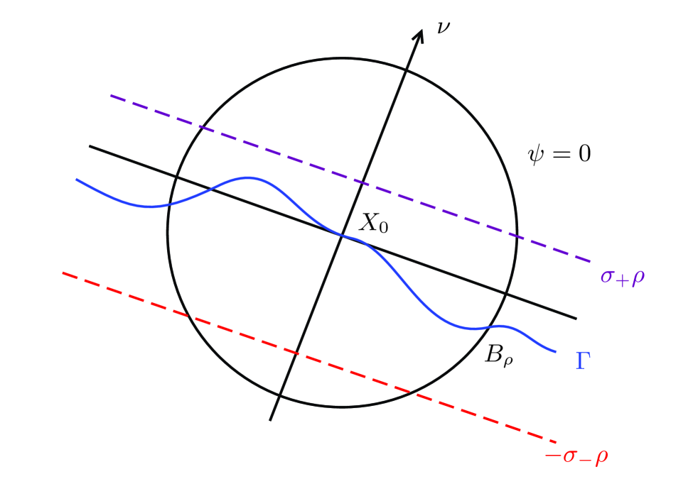
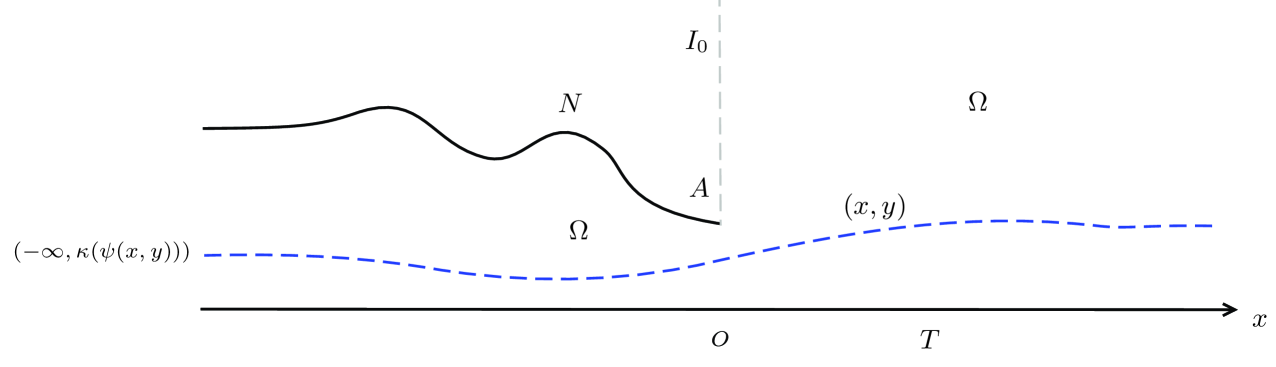
(Flat free boundary points) Let $\displaystyle 0<\sigma_{+},\sigma_{-}\leq 1$ and $\displaystyle\delta>0$ . We say that $\displaystyle\psi$ is of the flatness class $\displaystyle\mathcal{F}(\sigma_{+},\sigma_{-};\delta)$ in $\displaystyle B_{\rho}=B_{\rho}(X_{0})$ with a unit vector $\displaystyle\nu$ (see Figure 2) if

(i) $\displaystyle\psi$ is a minimizer to the variational problem $\displaystyle(P)$ .

(ii) $\displaystyle X_{0}\in\Gamma$ and

\psi(X)=0\ \ \text{for}\ \ (X-X_{0})\cdot\nu\geq\sigma_{+}\rho,

and

\psi(X)\geq-\lambda(X_{0})((X-X_{0})\cdot\nu+\sigma_{-}\rho)\ \ \text{for}\ \ (X-X_{0})\cdot\nu\leq-\sigma_{-}\rho.

(iii) $\displaystyle|\nabla\psi|\leq\lambda(X_{0})(1+\delta)$ in $\displaystyle B_{\rho}$ and $\displaystyle\sup_{X,Y\in B_{\rho}}|\lambda(X)-\lambda(Y)|\leq\lambda(X_{0})\delta$ .

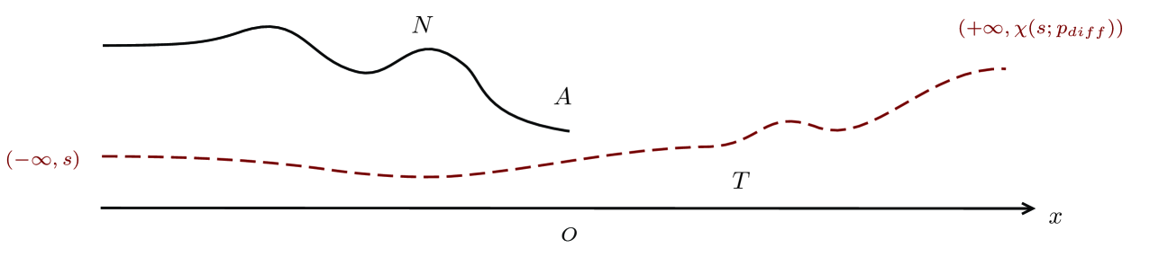
We next show that the flatness from above implies the flatness from below.

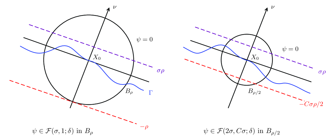
Lemma 3.8.

There exists a positive constant $\displaystyle C=C(\Lambda,c_{0})$ , such that for any small $\displaystyle\sigma>0$ , if $\displaystyle\psi\in\mathcal{F}(\sigma,1;\delta)$ in $\displaystyle B_{\rho}(X_{0})$ and $\displaystyle\delta\leq c_{0}\sigma,\rho\leq c_{0}\sigma$ , then $\displaystyle\psi\in\mathcal{F}(2\sigma,C\sigma;\delta)$ in $\displaystyle B_{\frac{\rho}{2}}(X_{0})$ (see Figure 3).

Proof.

We divide two steps to show this lemma.

Step 1. In this step, we will show that

\limsup_{X\rightarrow X_{0}}\frac{\psi(X)}{\text{dist}(X,B)}=\lambda(X_{0}),\ \text{if $\displaystyle B$ is a disc in $\displaystyle\{\psi=0\}$ touching $\displaystyle\partial\{\psi>0\}$ at $\displaystyle X_{0}$}.

(3.42)

Denote $\displaystyle\limsup_{X\rightarrow X_{0}}\frac{\psi(X)}{\text{dist}(X,B)}=\kappa$ , it suffices to show that $\displaystyle\kappa=\lambda(X_{0})$ . Taking a sequence $\displaystyle\{Y_{n}\}$ with $\displaystyle Y_{n}\rightarrow X_{0}$ , such that $\displaystyle\psi(Y_{n})>0$ , $\displaystyle d_{n}=\text{dist}(Y_{n},B)$ and

\frac{\psi(Y_{n})}{d_{n}}\rightarrow\kappa.

It follows from the non-degeneracy Lemma 2.6 that $\displaystyle\kappa>0$ . Consider a blow-up sequence $\displaystyle\psi_{n}(X)=\frac{\psi(X_{n}+d_{n}X)}{d_{n}}$ with respect to $\displaystyle B_{d_{n}}(X_{n})$ , where $\displaystyle X_{n}\in\partial B$ and $\displaystyle|X_{n}-Y_{n}|=d_{n}$ . Taking a subsequence $\displaystyle\{\psi_{n}\}$ with a blow-up limit $\displaystyle\psi_{0}\in C^{0,1}(\mathbb{R}^{2})$ , such that

\frac{X_{n}-Y_{n}}{d_{n}}\rightarrow\nu\ \ \text{and}\ \ \psi_{n}\rightarrow\psi_{0}\ \ \text{uniformly in any compact subset of $\displaystyle\mathbb{R}^{2}$}.

It is easy to check that $\displaystyle\psi_{0}(-\nu)=\kappa$ . We next claim that

\psi_{0}(X)=\kappa\max\{-X\cdot\nu,0\}.

(3.43)

In fact, the definition of $\displaystyle\psi_{0}$ gives that

\psi_{0}(X)\leq-\kappa X\cdot\nu\ \ \text{for}\ \ X\cdot\nu\leq 0,\ \ \text{and}\ \ \psi_{0}(X)=0\ \ \text{for}\ \ X\cdot\nu\geq 0.

Since $\displaystyle\psi_{0}$ is harmonic in $\displaystyle\{\psi_{0}>0\}$ and $\displaystyle\psi_{0}(-\nu)=\kappa$ , the strong maximum principle gives the claim (3.43).

With the aid of the claim (3.43), it follows from Lemma 3.7 that $\displaystyle\lambda(X_{0})=\kappa$ .

Step 2. Without loss of generality, we assume that $\displaystyle X_{0}=0$ and $\displaystyle\nu=e_{2}=(0,1)$ . Set $\displaystyle\psi_{\rho}(X)=\frac{\psi(\rho X)}{\rho}$ , $\displaystyle\lambda_{\rho}(X)=\lambda(\rho X)$ and $\displaystyle\lambda_{0}=\lambda(0)$ , one has

\Delta\psi_{\rho}+\rho f(\rho\psi_{\rho})=0\ \ \text{in}\ \ \{\psi_{\rho}>0\},\ \text{and $\displaystyle\psi_{\rho}\in F(\sigma,1;\delta)$ in $\displaystyle B_{1}$.}

(3.44)

Let

\eta(x)=\left\{\begin{array}[]{ll}0&\text{for}\ \ |x|\geq\frac{1}{3},\\ e^{-\frac{9x^{2}}{1-9x^{2}}}&\text{for}\ \ |x|<\frac{1}{3},\end{array}\right.

and choose $\displaystyle s\geq 0$ be the maximum with the property

B_{1}\cap\{\psi_{\rho}>0\}\subset D_{\sigma}=\{X\in B_{1}\mid y<\sigma-s\eta(x)\}.

Thus there exists a point $\displaystyle Z\in B_{\frac{1}{2}}\cap\partial D_{\sigma}\cap\partial\{\psi_{\rho}>0\}$ . It is easy to check that $\displaystyle s\leq\sigma$ , due to $\displaystyle 0\in\Gamma$ . Define a function $\displaystyle\phi(x,y)$ solving the problem

\left\{\begin{array}[]{ll}&\Delta\phi+\rho f(0)=0~~~~\text{in}~~D_{\sigma},\\ &\phi=0~~~~\text{on}~~\partial D_{\sigma}\cap B_{1},\ \ \ \ \ \phi=\lambda_{0}(1+2\sigma)(\sigma-y)~~~~\text{on}~~\partial D_{\sigma}\setminus B_{1}.\end{array}\right.

Noticing that $\displaystyle\lambda_{0}(1+2\sigma)(\sigma-y)+\lambda_{0}(1+\sigma)y\geq 0$ on $\displaystyle\partial D_{\sigma}$ , the maximum principle gives that

\phi(X)\geq-\lambda_{0}(1+\sigma)y\ \ \text{in}\ \ D_{\sigma}.

(3.45)

Next, we will show that

\partial_{-\nu}\phi(Z)\leq\lambda_{0}(1+C\sigma).

(3.46)

To see this, define a function $\displaystyle\phi_{1}$ as follows

\phi_{1}(x,y)=\frac{\mu_{2}}{\mu_{1}}\left(1-e^{-\mu_{1}g(x,y)}\right)\ \ \text{in}\ \ D_{\sigma},

where $\displaystyle g(x,y)=-y+\sigma-s\eta(x)$ and the constants $\displaystyle\mu_{1}$ and $\displaystyle\mu_{2}\geq\lambda_{0}$ depending on $\displaystyle\sigma$ will be determined later. It is easy to check that

1\leq|\nabla g(x,y)|\leq 1+C\sigma\ \ \text{and}\ \ |D^{2}g(x,y)|\leq C\sigma.

(3.47)

Therefore, it follows from (3.47) and $\displaystyle\rho\leq\sigma_{0}\sigma$ that

\Delta\phi_{1}+\rho f(0)=\mu_{2}e^{-\mu_{1}g}(\Delta g-\mu_{1}|\nabla g|^{2})+\rho f(0)\leq\mu_{2}e^{-\mu_{1}g}(C\sigma-\mu_{1})+\rho f(0)<0,

provided that

\mu_{1}=C_{1}\sigma,\ \ \text{$\displaystyle C_{1}$ is sufficiently large and $\displaystyle\sigma$ is small}.

On the other hand, take $\displaystyle\mu_{2}=\lambda_{0}(1+C_{2}\sigma)$ , $\displaystyle C_{2}$ is sufficiently large and $\displaystyle\sigma$ is small, one has

\phi_{1}(x,y)\geq\mu_{2}g(x,y)(1-C\mu_{1})\geq\lambda_{0}(1+2\sigma)g(x,y)\ \ \text{for any $\displaystyle(x,y)\in\partial D_{\sigma}$},

which together with the maximum principle gives that

\phi_{1}(X)\geq\phi(X)\ \ \text{in $\displaystyle D_{\sigma}$}.

Recalling that $\displaystyle\phi_{1}(Z)=\phi(Z)=0$ , we have

\partial_{-\nu}\phi(Z)\leq\partial_{-\nu}\phi_{1}(Z)\leq|\nabla\phi_{1}(Z)|=\mu_{2}|\nabla g(Z)|\leq\lambda_{0}(1+C\sigma),\ \ \text{$\displaystyle\sigma$ is small}.

In view of $\displaystyle\psi_{\rho}\in F(\sigma,1;\delta)$ , one has that $\displaystyle\psi_{\rho}\leq\phi$ on $\displaystyle\partial D_{\sigma}$ . The maximum principle gives that $\displaystyle\psi_{\rho}\leq\phi$ in $\displaystyle D_{\sigma}$ .

Consider the points $\displaystyle\xi\in\partial B_{\frac{3}{4}}$ with $\displaystyle\xi=(\xi_{1},\xi_{2})$ and $\displaystyle\xi_{2}<-\frac{1}{2}$ , and define a function $\displaystyle\varphi_{\xi}$ solving the following problem

\left\{\begin{array}[]{ll}&\Delta\varphi_{\xi}=0~~~~\text{in}~~D_{\sigma}\setminus B_{\frac{1}{10}}(\xi),\\ &\varphi_{\xi}=0~~~~\text{on}~~\partial D_{\sigma},\ \ \ \ \ \varphi_{\xi}=-\lambda_{0}y~~~~\text{on}~~\partial B_{\frac{1}{10}}(\xi).\end{array}\right.

Hopf’s Lemma gives that

\partial_{-\nu}\varphi_{\xi}(Z)\geq c\lambda_{0}>0.

(3.48)

Suppose that

\psi_{\rho}(X)\leq\phi(X)+\gamma\sigma\lambda_{0}y\ \ \text{for any $\displaystyle X\in B_{\frac{1}{10}}(\xi)$},

for a positive constant $\displaystyle\gamma>0$ . It should be noted that $\displaystyle\Delta(\psi_{\rho}-\phi+\gamma\sigma\varphi_{\xi})=-\rho f(\rho\psi_{\rho})+\rho f(0)\geq 0$ in $\displaystyle D_{\sigma}\setminus B_{\frac{1}{10}}(\xi)$ , and the maximum principle gives that

\psi_{\rho}\leq\phi-\gamma\sigma\varphi_{\xi}\ \ \ \ \text{in}\ \ D_{\sigma}\setminus B_{\frac{1}{10}}(\xi).

Therefore, we have

\lambda_{0}=\limsup_{X\rightarrow Z}\frac{\psi_{\rho}(X)}{\text{dist}(X,\partial D_{\sigma})}\leq\partial_{-\nu}\phi(Z)-\gamma\sigma\partial_{-\nu}\varphi_{\xi}(Z)\leq\lambda_{0}(1+C\sigma-c\gamma\sigma),

where $\displaystyle\nu$ is the outer normal vector and we have used (3.48). This leads a contradiction, provided that $\displaystyle\gamma$ is sufficiently large.

Hence, there exists some point $\displaystyle X_{\xi}=(x_{\xi},y_{\xi})\in B_{\frac{1}{10}}(\xi)$ , such that

\psi_{\rho}(X_{\xi})\geq\phi(X_{\xi})+C\sigma\lambda_{0}y_{\xi}.

(3.49)

For any $\displaystyle X\in B_{\frac{1}{5}}(\xi)$ , it follows from (3.45), (3.49) and (iii) in Definition 3.1 that

\psi_{\rho}(X)\geq\psi_{\rho}(X_{\xi})-\frac{3\lambda_{0}(1+\delta)}{10}\geq-\lambda_{0}(1+\sigma)y_{\xi}+C\sigma\lambda_{0}y_{\xi}-\frac{3\lambda_{0}(1+\delta)}{10}\geq\lambda_{0}\left(\frac{1}{10}-C\sigma\right)>0,

provided that $\displaystyle\sigma$ is small. Therefore, we have

\Delta(\phi-\psi_{\rho})=-\rho f(0)+\rho f(\rho\psi_{\rho})\ \ \text{and}\ \ \phi-\psi_{\rho}\geq 0\ \ \text{in}\ \ B_{\frac{1}{5}}(\xi).

Thanks to Harnack’s inequality in [31], one has

(\phi-\psi_{\rho})(\xi)\leq(\phi-\psi_{\rho})(X_{\xi})+C\rho\|f(0)-f(\rho\psi_{\rho})\|_{L^{\infty}(B_{1})}\leq C\lambda_{0}\sigma+C\sigma^{2}\leq C\lambda_{0}\sigma,

if $\displaystyle\sigma$ is small, which implies that

\psi_{\rho}(\xi)\geq\phi(\xi)-C\lambda_{0}\sigma\geq\lambda_{0}(-(1+\sigma)\xi_{2}-C\sigma\geq-\xi_{2}-C\sigma.

(3.50)

It follows from (3.50) and $\displaystyle(iii)$ in Definition 3.1 that

\psi_{\rho}(\xi+te_{2})\geq\psi_{\rho}(\xi)-\lambda_{0}(1+\delta)t\geq\lambda_{0}(-(\xi_{2}+t)-C\sigma),

for $\displaystyle t>0$ and $\displaystyle\xi+te_{2}\in B_{\frac{1}{2}}$ , which implies that $\displaystyle\psi_{\rho}$ is of $\displaystyle\mathcal{F}(2\sigma,C\sigma;\delta)$ in $\displaystyle B_{\frac{1}{2}}$ . This completes the proof of this lemma. ∎

In the following, denote $\displaystyle B_{r}=B_{r}(0)$ , we will investigate the blow-up limit. Thanks to Lemma 7.3 and Corollary 7.4 in [2], we have the following non-homogeneous blow-up limit and we omit the proof here.

Lemma 3.9.

(Non-homogenous blow up)Let $\displaystyle\psi_{n}\in\mathcal{F}(\sigma_{n},\sigma_{n};\delta_{n})$ in $\displaystyle B_{\rho_{n}}$ with $\displaystyle v=e_{2}$ , $\displaystyle\sigma_{n}\rightarrow 0$ , $\displaystyle\delta_{n}\sigma^{-2}_{n}\rightarrow 0$ and $\displaystyle\rho_{n}\sigma_{n}^{-1}\rightarrow 0$ . For any $\displaystyle x\in(-1,1)$ , set

b^{+}_{n}(x)=\sup\{h\mid(\rho_{n}x,\sigma_{n}\rho_{n}h)\in\partial\{\psi_{n}>0\}\},

and

b^{-}_{n}(x)=\inf\{h\mid(\rho_{n}x,\sigma_{n}\rho_{n}h)\in\partial\{\psi_{n}>0\}\},

then for a subsequence,

b(x)=\limsup_{z\rightarrow x,n\rightarrow\infty}b_{n}^{+}(z)=\liminf_{z\rightarrow x,n\rightarrow\infty}b_{n}^{-}(z)\ \ \text{for any $\displaystyle x\in(-1,1)$}.

Furthermore, $\displaystyle b_{n}^{+}(x)\rightarrow b(x)$ and $\displaystyle b_{n}^{-}(x)\rightarrow b(x)$ uniformly in $\displaystyle(-1,1)$ , $\displaystyle b(0)=0$ and $\displaystyle b(x)$ is a continuous function.

Furthermore, we can show that the limit function $\displaystyle b(x)$ is a convex function.

Lemma 3.10.

$\displaystyle b(x)$ is convex with respect to $\displaystyle x$ .

Proof.

Set $\displaystyle\psi_{n}(X)=\frac{\psi(\rho_{n}X)}{\rho_{n}}$ , $\displaystyle\lambda_{n}(X)=\lambda(\rho_{n}X)$ and $\displaystyle\lambda_{0}=\lambda(0)$ , one has

\Delta\psi_{n}+\rho_{n}f(\rho_{n}\psi_{n})=0\ \ \text{in}\ \ \{\psi_{n}>0\}\ \ \text{and $\displaystyle\psi_{n}\in\mathcal{F}(\sigma_{n},\sigma_{n};\delta_{n})$ in $\displaystyle B_{1}$}.

If the assertion is not true, there exists a $\displaystyle x_{0}\in(-1,1)$ and a linear function $\displaystyle g(x)$ in $\displaystyle I_{\rho}=(-\rho+x_{0},\rho+x_{0})\subset(-1,1)$ , such that

g(x_{0}\pm\rho)>b(x_{0}\pm\rho)\ \ \text{ and}\ b(x_{0})>g(x_{0}).

Denote

\mathcal{D}=I_{\rho}\times\mathbb{R}\ \text{and}\ \mathcal{D}^{+}(k)=\{(x,y)\in\mathcal{D}\mid k(x)<y<g_{0}+2\},

and

\mathcal{D}^{0}(k)=\{(x,y)\in\mathcal{D}\mid y=k(x)\}\ \text{and}\ \mathcal{D}^{-}(k)=\{(x,y)\in\mathcal{D}\mid y<k(x)\},

for continuous function $\displaystyle k(x)$ , where $\displaystyle g_{0}=\max\{g(x_{0}-\rho),g_{0}(x_{0}+\rho)\}$ . Define a test function $\displaystyle d_{\varepsilon,E}(X)=\min\left\{\frac{\text{dist}(X,\mathbb{R}^{2}\setminus E)}{\varepsilon},1\right\}$ for a set $\displaystyle E$ , it is easy to check that $\displaystyle d_{\varepsilon,E}(X)$ converges to the characteristic function $\displaystyle I_{E}(X)$ as $\displaystyle\varepsilon\rightarrow 0$ .

It follows from Proposition 3.3 that

\begin{array}[]{rl}&-\int_{\Omega_{n}}\nabla\psi_{n}\cdot\nabla d_{\varepsilon,E}(\mathcal{D}^{+}(\sigma_{n}g))dX+\int_{\Omega_{n}\cap\{\psi_{n}>0\}}\rho_{n}f(\rho_{n}\psi_{n})d_{\varepsilon,E}(\mathcal{D}^{+}(\sigma_{n}g))dX\\ =&\int_{\Omega_{n}\cap\partial_{red}\{\psi_{n}>0\}}d_{\varepsilon,E}(\mathcal{D}^{+}(\sigma_{n}g))\lambda_{n}d\mathcal{H}^{1},\end{array}

(3.51)

where $\displaystyle\Omega_{n}=\{X\mid\rho_{n}X\in\Omega\}$ .

Taking $\displaystyle\varepsilon\rightarrow 0$ in (3.51), one has

\begin{array}[]{rl}&-\int_{\partial\mathcal{D}^{+}(\sigma_{n}g)\cap\{\psi_{n}>0\}}\nabla\psi_{n}\cdot\nu d\mathcal{H}^{1}+\int_{\mathcal{D}^{+}(\sigma_{n}g)\cap\{\psi_{n}>0\}}\rho_{n}f(\rho_{n}\psi_{n})dX\\ =&\int_{\mathcal{D}^{+}(\sigma_{n}g)\cap\partial_{red}\{\psi_{n}>0\}}\lambda_{n}d\mathcal{H}^{1},\end{array}

which gives that

\begin{array}[]{rl}&\mathcal{H}^{1}(\mathcal{D}^{+}(\sigma_{n}g)\cap\partial_{red}\{\psi_{n}>0\})\\ \leq&\frac{1}{\lambda_{0}(1-\delta_{n})}\int_{\mathcal{D}^{+}(\sigma_{n}g)\cap\partial_{red}\{\psi_{n}>0\}}\lambda_{n}d\mathcal{H}^{1}\\ \leq&\frac{1}{\lambda_{0}(1-\delta_{n})}\left(\int_{\partial\mathcal{D}^{+}(\sigma_{n}g)\cap\{\psi_{n}>0\}}|\nabla\psi_{n}|d\mathcal{H}^{1}+C\rho_{n}\int_{\mathcal{D}^{+}(\sigma_{n}g)\cap\{\psi_{n}>0\}}dX\right)\\ \leq&\frac{1+\delta_{n}}{1-\delta_{n}}\mathcal{H}^{1}(\mathcal{D}^{0}(\sigma_{n}g)\cap\{\psi_{n}>0\})+\frac{C\rho_{n}\sigma_{n}}{\lambda_{0}(1-\delta_{n})}.\end{array}

(3.52)

Denote

E_{n}=\{\psi_{n}>0\}\cup\mathcal{D}^{-}(\sigma_{n}g).

It is easy to check that $\displaystyle E_{n}$ has finite perimeter in $\displaystyle\mathcal{D}$ and

\begin{array}[]{rl}\mathcal{H}^{1}(\mathcal{D}\cap\partial_{red}E_{n})\leq\mathcal{H}^{1}(\mathcal{D}^{+}(\sigma_{n}g)\cap\partial_{red}\{\psi_{n}>0\})+\mathcal{H}^{1}(\mathcal{D}^{0}(\sigma_{n}g)\cap\{\psi_{n}=0\}).\end{array}

(3.53)

By using the similar estimate in Page 136-Page 137 in [2], one has

\begin{array}[]{rl}\mathcal{H}^{1}(\mathcal{D}\cap\partial_{red}E_{n})\geq\mathcal{H}^{1}(\mathcal{D}^{0}(\sigma_{n}g))+c\sigma_{n}^{2}.\end{array}

(3.54)

It follows from (3.52)-(3.54) that

\begin{array}[]{rl}&\mathcal{H}^{1}(\mathcal{D}^{0}(\sigma_{n}g))+c\sigma_{n}^{2}\leq\frac{1+\delta_{n}}{1-\delta_{n}}\mathcal{H}^{1}(\mathcal{D}^{0}(\sigma_{n}g))+\frac{C\rho_{n}\sigma_{n}}{\lambda_{0}(1-\delta_{n})},\end{array}

(3.55)

that is

0<c\leq\frac{2\delta_{n}\sigma_{n}^{-2}}{1-\delta_{n}}\mathcal{H}^{1}(\mathcal{D}^{0}(\sigma_{n}g))+\frac{C\rho_{n}\sigma_{n}^{-1}}{\lambda_{0}(1-\delta_{n})},

which contradicts to the facts $\displaystyle\rho_{n}\sigma_{n}^{-1}\rightarrow 0$ and $\displaystyle\delta_{n}\sigma^{-2}_{n}\rightarrow 0$ .

∎

With the aid of Lemma 3.10, based on Lemma 7.6 in [2] and Lemma 5.6 in [6], we will show that

Lemma 3.11.

There exists a constant $\displaystyle C$ , such that for any $\displaystyle x\in\left(-\frac{1}{2},\frac{1}{2}\right)$ ,

\int_{0}^{\frac{1}{4}}\frac{1}{r^{2}}(\text{Av}_{r}(b(x))-b(x))dr\leq C,

where $\displaystyle\text{Av}_{r}(b(x))=\frac{b(x+r)+b(x-r)}{2}$ .

Proof.

Set $\displaystyle\psi_{n}(X)=\frac{\psi(\rho_{n}X)}{\rho_{n}}$ , $\displaystyle\lambda_{n}(X)=\lambda(\rho_{n}X)$ and $\displaystyle\lambda_{0}=\lambda(0)$ , one has

\Delta\psi_{n}+\rho_{n}f(\rho_{n}\psi_{n})=0\ \ \text{in}\ \ \{\psi_{n}>0\},\ \ \text{and $\displaystyle\psi_{n}\in\mathcal{F}(\sigma_{n},\sigma_{n};\delta_{n})$ in $\displaystyle B_{1}$}.

(3.56)

It is easy to check that $\displaystyle\psi_{n}$ be the class of $\displaystyle\mathcal{F}(8\sigma_{n},8\sigma_{n};\delta_{n})$ in $\displaystyle B_{\frac{1}{4}}(x,\sigma_{n}b_{n}^{+}(x))$ , provided that $\displaystyle n$ is sufficiently large. Therefore, it suffices to show the lemma for $\displaystyle x=0$ , that is

\int_{0}^{\frac{1}{4}}\frac{1}{r^{2}}(\text{Av}_{r}(b(0)))dr\leq C.

(3.57)

Set

\phi_{n}(x,y)=\frac{\psi_{n}(x,y)+\lambda_{0}y}{\sigma_{n}}.

Recalling the flatness condition for $\displaystyle\psi_{n}$ , the free boundary of $\displaystyle\psi_{n}$ lies in the strip $\displaystyle|y|\leq c\sigma_{n}$ . Since $\displaystyle|\nabla\psi_{n}|\leq\lambda_{0}(1+\delta_{n})$ and $\displaystyle\delta_{n}\leq\sigma_{n}$ , we have

\displaystyle\phi_{n}\leq C

\displaystyle B_{1}^{-}=B_{1}\cap\{y<0\}

The flatness condition implies that $\displaystyle\phi_{n}\geq-C$ in $\displaystyle B_{1}^{-}$ . Therefore, one has

|\phi_{n}|\leq C\ \ \text{in}\ \ B_{1}^{-}.

(3.58)

It is easy to check that

\Delta\phi_{n}=\frac{\rho_{n}}{\sigma_{n}}f(\rho_{n}(\sigma_{n}\phi_{n}-\lambda_{0}y))\ \ \text{in}\ \ B_{1}^{-}\cap\{y<-\sigma_{n}\}.

(3.59)

Thanks to the flatness conditions on $\displaystyle\psi_{n}$ and Lemma 3.7, there exists a subsequence still labeled by $\displaystyle\{\psi_{n}\}$ , such that

\psi_{n}(x,y)\rightarrow-\lambda_{0}y\ \ \text{in $\displaystyle C^{2}$ in any compact subset of $\displaystyle B_{1}^{-}$}.

In view of (3.58), we can conclude that

\phi_{n}\rightarrow\phi\ \ \text{in $\displaystyle C^{2}$ in compact subsets of $\displaystyle B_{1}^{-}$}.

(3.60)

Since $\displaystyle\rho_{n}\sigma_{n}^{-1}\rightarrow 0$ , it follows from (3.59) and (3.60) that

\Delta\phi=0\ \ \text{in}\ \ B_{1}^{-},\ \ \text{and}\ \ |\phi|\leq C.

(3.61)

By virtue of $\displaystyle\phi_{n}(0,0)=0$ , we have that for any $\displaystyle y\leq 0$ , there exists a $\displaystyle\xi\in(y,0)$ , such that

\phi_{n}(0,y)\leq\frac{\partial\phi_{n}(0,\xi)}{\partial y}y=\frac{1}{\sigma_{n}}\left(\frac{\partial\psi_{n}(0,\xi)}{\partial y}+\lambda_{0}\right)y\leq\frac{|\nabla\psi_{n}|-\lambda_{0}}{\sigma_{n}}|y|\leq\frac{\lambda_{0}\delta_{n}}{\sigma_{n}}|y|\rightarrow 0.

(3.62)

Then it gives that

\phi(0,y)\leq 0\ \ \text{for any $\displaystyle y\leq 0$}.

(3.63)

Next, we will show that

\phi(x,0)=\lambda_{0}b(x)\ \ \text{in the sense that $\displaystyle\lim_{y\uparrow 0}\phi(x,y)=\lambda_{0}b(x)$}.

(3.64)

To obtain the fact (3.64), we first show that for any small $\displaystyle\eta>0$ and any large constant $\displaystyle M$ , we have

\phi_{n}(x,y\sigma_{n})\rightarrow\lambda_{0}b(x)\ \ \text{uniformly for $\displaystyle x\in I_{\eta}=(-1+\eta,1-\eta)$ and $\displaystyle-M\leq y\leq-1$},

(3.65)

as $\displaystyle n\rightarrow\infty$ .

On another hand, to see this, thanks to the non-homogeneous blow-up Lemma 3.9, it suffices to show that

\phi_{n}(x,h\sigma_{n})-\lambda_{0}b_{n}^{+}(x)\rightarrow 0.

(3.66)

It follows from (3.62) that for any $\displaystyle x\in I_{\eta}$ , one has

\begin{array}[]{rl}\phi_{n}(x,y\sigma_{n})-\lambda_{0}b_{n}^{+}(x)=&\phi_{n}(x,\sigma_{n}b_{n}^{+}(x))-\lambda_{0}b_{n}^{+}(x)+\frac{\partial\phi_{n}(0,\xi)}{\partial y}\sigma_{n}(y-b_{n}^{+}(x))\\ \leq&\delta_{n}(b_{n}^{+}(x)-y)\leq(1+M)\delta_{n}\rightarrow 0,\end{array}

(3.67)

as $\displaystyle n\rightarrow\infty$ , where we have used the fact

\phi_{n}(x,\sigma_{n}b_{n}^{+}(x))-\lambda_{0}b_{n}^{+}(x)=\frac{\psi_{n}(x,\sigma_{n}b_{n}^{+}(x))+\lambda_{0}\sigma_{n}b_{n}^{+}(x)}{\sigma_{n}}-\lambda_{0}b_{n}^{+}(x)=\frac{\psi_{n}(x,\sigma_{n}b_{n}^{+}(x))}{\sigma_{n}}=0.

Taking any sequence $\displaystyle\{x_{n}\}$ with $\displaystyle x_{n}\in I_{\eta}$ and $\displaystyle-M\leq h_{n}\leq-1$ , and consider $\displaystyle\psi_{n}$ in $\displaystyle B_{R\sigma_{n}}(X_{n})$ , where $\displaystyle X_{n}=(x_{n},\sigma_{n}b_{n}^{+}(x_{n}))$ is the free boundary point and $\displaystyle R$ is an arbitrary large constant. Denote $\displaystyle\tilde{\sigma}_{n}=\frac{1}{R}\sup_{x\in I_{R\sigma_{n}}}(b_{n}^{+}(x)-b_{n}^{+}(x_{n}))$ with $\displaystyle I_{R\sigma_{n}}=(x_{n}-R\sigma_{n},x_{n}+R\sigma_{n})$ . It follows from Lemma 3.9 that $\displaystyle\tilde{\sigma}_{n}\rightarrow 0$ . Next, we claim that

\psi_{n}\in\mathcal{F}(\tilde{\sigma}_{n},1;C_{1}\delta_{n})\ \ \text{in}\ \ B_{R\sigma_{n}}(X_{n}),

(3.68)

where $\displaystyle C_{1}$ is a constant depending on $\displaystyle\lambda_{1}$ and $\displaystyle\lambda_{2}$ , provided that $\displaystyle n$ is sufficiently large. In fact, the definition of $\displaystyle b^{+}_{n}(x)$ gives that

\text{ $\displaystyle\psi_{n}(x,y)=0\ $ for $\displaystyle\ y\geq\sigma_{n}b_{n}^{+}(x_{n})+\tilde{\sigma}_{n}R\sigma_{n}$}.

Since $\displaystyle|\nabla\psi_{n}(X)|\leq\lambda_{0}(1+\delta_{n})$ in $\displaystyle B_{1}(0)$ and $\displaystyle\sup_{X,Y\in B_{1}(0)}|\lambda_{n}(X)-\lambda_{n}(Y)|\leq\lambda_{0}\delta_{n},$ we have that

|\nabla\psi_{n}(X)|\leq(\lambda_{n}(X_{n})+\lambda_{0}\delta_{n})(1+\delta_{n})\leq\lambda_{n}(X_{n})\left(1+C_{1}\delta_{n}\right)\ \ \text{in $\displaystyle B_{R\sigma_{n}}(X_{n})$,}

and

\sup_{X,Y\in B_{R\sigma_{n}}(X_{n})}|\lambda_{n}(X)-\lambda_{n}(Y)|\leq\lambda_{0}\delta_{n}\leq(\lambda_{n}(X_{n})+\lambda_{0}\delta_{n})\delta_{n}\leq\lambda_{n}(X_{n})C_{1}\delta_{n},

where $\displaystyle C_{1}$ is a constant depending on $\displaystyle\lambda_{1}$ and $\displaystyle\lambda_{2}$ . Therefore, we obtain the claim (3.68).

In view of the claim (3.68), by virtue of the flatness Lemma 3.8, we have

\psi_{n}\in\mathcal{F}(2\bar{\sigma}_{n},C\bar{\sigma}_{n};C_{1}\delta_{n})\ \ \text{in}\ \ B_{\frac{R\sigma_{n}}{2}}(X_{n}),

(3.69)

provided that $\displaystyle\bar{\sigma}_{n}=\max\{\tilde{\sigma}_{n},\delta_{n}\}$ .

Hence, for any $\displaystyle h$ with $\displaystyle|h|<\frac{R}{2}$ , it follows from (3.69) that

\psi_{n}(X_{n}+h\sigma_{n}e_{2})\geq-\lambda_{n}(X_{n})\left(h\sigma_{n}+\frac{C\bar{\sigma}_{n}R\sigma_{n}}{2}\right),

that is

\begin{array}[]{rl}\phi_{n}(X_{n}+h\sigma_{n}e_{2})-\lambda_{0}b_{n}^{+}(x_{n})=&\frac{\psi_{n}(X_{n}+h\sigma_{n}e_{2})+\lambda_{0}h\sigma_{n}}{\sigma_{n}}\\ \geq&(\lambda(0)-\lambda(\rho_{n}X_{n}))h-\frac{C\lambda(\rho_{n}X_{n})\bar{\sigma}_{n}R}{2}\rightarrow 0.\end{array}

This together with (3.67) gives (3.66).

For any $\displaystyle\varepsilon>0$ , let $\displaystyle\varphi_{\varepsilon}$ be the solution of the Dirichlet problem

\left\{\begin{array}[]{ll}&\Delta\varphi_{\varepsilon}=1~~~~\text{in}~~B_{1-\eta}^{-},\\ &\varphi_{\varepsilon}=\lambda_{0}b(x)-\varepsilon~~~~\text{on}~~\partial B_{1-\eta}^{-}\cap\{y=0\},\ \ \ \ \ \varphi_{\varepsilon}=\inf_{B_{1}^{-}}\phi~~~~\text{on}~~\partial B_{1-\eta}^{-}\cap\{y<0\}.\end{array}\right.

It follows from (3.65) that

\phi_{n}>\varphi_{\varepsilon}\ \ \text{on}\ \ \partial(B_{1-\eta}^{-}\cap\{y<-M\sigma_{n}\}),

(3.70)

for any large constant $\displaystyle M$ (independent of $\displaystyle\eta$ and $\displaystyle\varepsilon$ ), provided that $\displaystyle n$ is sufficiently large (depending on $\displaystyle\varepsilon$ and $\displaystyle M$ ). Moreover,

\Delta(\varphi_{\varepsilon}-\phi_{n})=1+\frac{\rho_{n}}{\sigma_{n}}f(\rho_{n}(\sigma_{n}\phi_{n}-\lambda_{0}y))>0\ \text{ in $\displaystyle B_{1-\eta}^{-}\cap\{y<-M\sigma_{n}\}$},

provided that $\displaystyle n$ is sufficiently large. In view of (3.70), the maximum principe gives that

\varphi_{\varepsilon}\leq\phi_{n}\ \ \text{ in $\displaystyle B_{1-\eta}^{-}\cap\{y<-M\sigma_{n}\}$, if $\displaystyle n$ is large enough}.

(3.71)

Taking $\displaystyle n\rightarrow\infty$ in (3.71), we have

\varphi_{\varepsilon}(x,y)\leq\phi(x,y)\ \ \text{ in $\displaystyle B_{1-\eta}^{-}$}.

Consequently,

\lambda_{0}b(x)-2\varepsilon\leq\lim_{y\uparrow 0}\varphi_{\varepsilon}(x,y)\leq\liminf_{y\uparrow 0}\phi(x,y)\ \ \text{ for $\displaystyle x\in(-1+2\eta,1-2\eta)$ and $\displaystyle\eta>0$}.

(3.72)

Similarly, by working with a solution $\displaystyle\tilde{\varphi}_{\varepsilon}(x,y)$ to the Dirichlet problem

\left\{\begin{array}[]{ll}&\Delta\tilde{\varphi}_{\varepsilon}=-1~~~~\text{in}~~B_{1-\eta}^{-},\\ &\tilde{\varphi}_{\varepsilon}=\lambda_{0}b(x)+\varepsilon~~~~\text{on}~~\partial B_{1-\eta}^{-}\cap\{y=0\},\ \ \ \ \ \tilde{\varphi}_{\varepsilon}=\sup_{B_{1}^{-}}\phi~~~~\text{on}~~\partial B_{1-\eta}^{-}\cap\{y<0\},\end{array}\right.

for any $\displaystyle\varepsilon>0$ , we can obtain that

\lambda_{0}b(x)+2\varepsilon\geq\limsup_{y\uparrow 0}\phi(x,y)\ \ \text{ for $\displaystyle x\in(-1+2\eta,1-2\eta)$}.

(3.73)

By virtue of the arbitrariness of $\displaystyle\varepsilon$ , it follows from (3.72) and (3.73) that we obtain the claim (3.64).

In view of Lemma 3.10, (3.58), (3.61),(3.63) and (3.64), we can apply Lemma 5.5 in [6] to obtain (3.57). ∎

With the aid of Lemma 3.11, it follows from Lemma 7.7 - Lemma 7.9 in [2] that the flatness from below implies the flatness from above (see Figure 4).

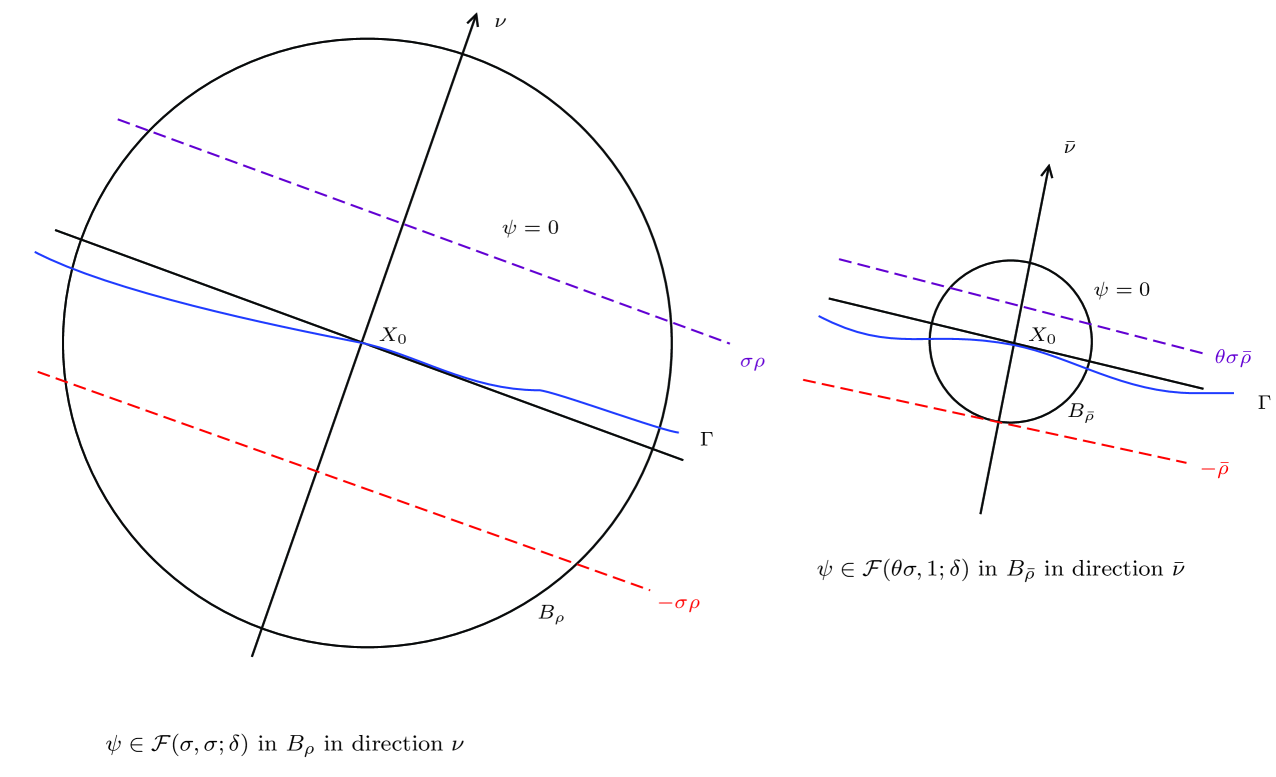
Lemma 3.12.

For any $\displaystyle\theta>0$ , there exist a large constant $\displaystyle C$ , $\displaystyle c_{\theta}=c(\theta)$ and a small $\displaystyle\sigma_{\theta}=\sigma(\theta)$ , such that if

\psi\in\mathcal{F}(\sigma,\sigma;\delta)\ \ \text{in $\displaystyle B_{\rho}$ in direction $\displaystyle\nu$ with $\displaystyle\sigma\leq\sigma_{\theta},\delta\leq\sigma_{\theta}\sigma^{2},\rho\leq\sigma_{\theta}\sigma$},

then

\psi\in\mathcal{F}(\theta\sigma,1;\delta)\ \ \text{in $\displaystyle B_{\bar{\rho}}$ in direction $\displaystyle\bar{\nu}$ for some $\displaystyle\bar{\rho}$ and $\displaystyle\bar{\nu}$ with $\displaystyle c_{\theta}\rho\leq\bar{\rho}\leq\theta\rho$ and $\displaystyle|\nu-\bar{\nu}|\leq C\sigma$}.

By virtue of Lemma 3.8 and Lemma 3.12, we will show that

Lemma 3.13.

Let $\displaystyle\omega(s)$ be a monotone increasing and continuous function with $\displaystyle\omega(0)=0$ . For any $\displaystyle\theta\in(0,1)$ , there exists a small $\displaystyle\sigma_{0}>0$ , such that if

\psi\in\mathcal{F}(\sigma,1;\delta)\ \ \text{in $\displaystyle B_{\rho}$ in direction $\displaystyle\nu$ with $\displaystyle\sigma\leq\sigma_{0},\ \delta\leq\sigma_{0}\sigma^{2},\ \rho\leq\sigma_{0}\sigma$},

and $\displaystyle\sup_{X,Y\in B_{s\rho}}|\lambda(X)-\lambda(Y)|\leq\omega(s)\lambda(0)\delta$ for $\displaystyle s\in[0,1]$ , then there exist a large constant $\displaystyle C$ and $\displaystyle c_{\theta}=c(\theta,\omega)$ , such that

\psi\in\mathcal{F}(\theta\sigma,\theta\sigma;\theta^{2}\delta)\ \ \text{in $\displaystyle B_{\bar{\rho}}$ in direction $\displaystyle\bar{\nu}$}

for some $\displaystyle\bar{\rho}$ and $\displaystyle\bar{\nu}$ , where $\displaystyle c_{\theta}\rho\leq\bar{\rho}\leq\frac{1}{4}\rho$ and $\displaystyle|\nu-\bar{\nu}|\leq C\sigma$ .

Proof.

Step 1. By virtue of Lemma 3.8, one has

\psi\in\mathcal{F}(C_{0}\sigma,C_{0}\sigma;\delta)\ \ \text{in $\displaystyle B_{\frac{\rho}{2}}$ in direction $\displaystyle\nu$, where $\displaystyle C_{0}>2$.}

Then for some small $\displaystyle\theta_{1}\in\left(0,1/2\right]$ to be determined later, it follows from Lemma 3.12 that

\psi\in\mathcal{F}(C_{0}\theta_{1}\sigma,1;\delta)\ \ \text{in $\displaystyle B_{\rho_{1}}$ in direction $\displaystyle\nu_{1}$ for some $\displaystyle\rho_{1}$ and $\displaystyle\nu_{1}$},

where

\text{$\displaystyle c_{\theta_{1}}\frac{\rho}{2}\leq\rho_{1}\leq\theta_{1}\frac{\rho}{2}$ and $\displaystyle|\nu-\nu_{1}|\leq C\sigma$}.

To improve the value of $\displaystyle\delta$ , we define

U(X)=\max\left\{|\nabla\psi(X)|-\sup_{X\in B_{3\rho_{1}}}\lambda(X),0\right\}\ \ \text{in}\ \ B_{2\rho_{1}}\cap\{\psi>0\}.

It is easy to check that

\Delta U=\frac{|D^{2}\psi||\nabla\psi|^{2}-\partial_{k}\psi\partial_{j}\psi\partial_{ij}\psi\partial_{ik}\psi}{|\nabla\psi|^{3}}-f^{\prime}(\psi)|\nabla\psi|\geq 0\ \ \text{in}\ \ B_{2\rho_{1}}\cap\{\psi>0\}.

For subharmonic function $\displaystyle U$ , we can use the similar arguments in P141 in [2] and obtain that there exists a $\displaystyle c\in(0,1)$ , such that

U(X)=\max\left\{|\nabla\psi(X)|-\sup_{X\in B_{3\rho_{1}}}\lambda(X),0\right\}\leq(1-c)\lambda(0)\delta\ \ \text{in}\ \ B_{\rho_{1}},

which implies that

|\nabla\psi(X)|\leq\sup_{X\in B_{3\rho_{1}}}\lambda(X)+\lambda(0)(1-c)\delta\leq\lambda(0)+\lambda(0)(1-c+w(2\theta_{1}))\delta\ \ \text{in}\ \ B_{\rho_{1}}.

Denote

\theta_{0}=\sqrt{1-\frac{c}{2}}.

Taking $\displaystyle\theta_{1}$ be sufficiently small, such that $\displaystyle\frac{\theta_{1}}{2\theta_{0}}<1$ and $\displaystyle C_{0}\theta_{1}<\theta_{0}$ , then the continuity of $\displaystyle\omega(s)$ gives that

\omega(2\theta_{1})\leq\frac{c}{2}\ \ \text{and}\ \ \omega\left(\frac{\theta_{1}}{2}\right)<\theta_{0}^{2}.

Furthermore,

|\nabla\psi(X)|\leq\lambda(0)+\lambda(0)\left(1-\frac{c}{2}\right)\delta\leq\lambda(0)(1+\theta_{0}^{2}\delta)\ \ \text{in}\ \ B_{\rho_{1}},

and

\sup_{X,Y\in B_{\rho_{1}}}|\lambda(X)-\lambda(Y)|\leq\sup_{X,Y\in B_{\frac{\theta_{1}}{2}\rho}}|\lambda(X)-\lambda(Y)|\leq\omega\left(\frac{\theta_{1}}{2}\right)\lambda(0)\delta\leq\theta_{0}^{2}\lambda(0)\delta.

Thus we have

\psi\in\mathcal{F}(\theta_{0}\sigma,1;\theta_{0}^{2}\delta)\ \ \text{in $\displaystyle B_{\rho_{1}}$ in direction $\displaystyle\nu_{1}$}.

On the other hand, we have

\sup_{X,Y\in B_{s\rho_{1}}}|\lambda(X)-\lambda(Y)|\leq\omega_{1}(s)\theta_{0}^{2}\lambda(0)\delta\ \ \text{and}\ \ \omega_{1}(s)=\theta_{0}^{-2}\omega\left(\frac{\theta_{1}}{2}s\right)\leq\theta_{0}^{-2}\omega\left(\frac{\theta_{1}}{2}\right)<1.

Notice that

\rho_{1}\leq\theta_{1}\frac{\rho}{2}\leq\left(\frac{\theta_{1}}{2\theta_{0}}\sigma_{0}\right)\theta_{0}\sigma<\sigma_{0}(\theta_{0}\sigma)\ \ \text{and}\ \ \theta^{2}_{0}\delta\leq\sigma_{0}(\theta_{0}\sigma)^{2},

due to $\displaystyle\frac{\theta_{1}}{2\theta_{0}}<1$ and $\displaystyle\rho\leq\sigma_{0}\sigma$ .

Step 2. Repeating the arguments in Step 1, and choosing sufficiently small $\displaystyle\sigma_{0}>0$ , we obtain

\psi\in\mathcal{F}(\theta^{2}_{0}\sigma,1;\theta_{0}^{4}\delta)\ \ \text{in $\displaystyle B_{\rho_{2}}$ in direction $\displaystyle\nu_{2}$},

for some $\displaystyle\rho_{2}$ and $\displaystyle\nu_{2}$ , where

\text{$\displaystyle c_{\theta_{1}}\frac{\rho_{1}}{2}\leq\rho_{2}\leq\theta_{1}\frac{\rho_{1}}{2}$ and $\displaystyle|\nu_{2}-\nu_{1}|\leq C\theta_{0}\sigma$}.

Similarly, we can repeat the arguments in Step 1 for a finite number $\displaystyle n$ , and we choose the constant $\displaystyle\sigma_{0}$ being small enough in the statement for each step, thus

\psi\in\mathcal{F}(\theta^{n}_{0}\sigma,1;\theta_{0}^{2n}\delta)\ \ \text{in $\displaystyle B_{\rho_{n}}$ in direction $\displaystyle\nu_{n}$},

(3.74)

for some $\displaystyle\rho_{n}$ and $\displaystyle\nu_{n}$ , where

\text{$\displaystyle c_{\theta_{1}}\frac{\rho_{n-1}}{2}\leq\rho_{n}\leq\theta_{1}\frac{\rho_{n-1}}{2}$ and $\displaystyle|\nu_{n}-\nu_{n-1}|\leq C\theta^{n-1}_{0}\sigma$}.

(3.75)

Applying Lemma 3.8 again, we have

\psi\in\mathcal{F}(2\theta_{0}^{n}\sigma,C\theta_{0}^{n}\sigma;\theta_{0}^{2n}\delta)\ \ \text{in $\displaystyle B_{\frac{\rho_{n}}{2}}$ in direction $\displaystyle\nu_{n}$.}

Choosing $\displaystyle N=N(\theta)$ as the smallest positive integer such that

\max\left\{2\theta_{0}^{N},C\theta_{0}^{N}\right\}\leq\theta,

where the constant $\displaystyle C$ is obtained in Lemma 3.8. It follows from (3.75) that

\text{$\displaystyle\frac{c^{N}_{\theta_{1}}}{2^{N}}\rho\leq\rho_{N}\leq\frac{\theta_{1}^{N}}{2^{N}}\rho$ and $\displaystyle|\nu_{N}-\nu|\leq\frac{C\sigma}{1-\theta_{0}}$}.

(3.76)

Then we have

\psi\in\mathcal{F}(\theta\sigma,\theta\sigma;\theta^{2}\delta)\ \ \text{in $\displaystyle B_{\bar{\rho}}$ in direction $\displaystyle\bar{\nu}$,}

where $\displaystyle\bar{\rho}=\frac{\rho_{N}}{2}$ and $\displaystyle\bar{\nu}=\nu_{N}$ . Denote $\displaystyle c_{\theta}=\frac{c^{N}_{\theta_{1}}}{2^{N(\theta)+1}}$ , it follows from (3.76) that

\text{$\displaystyle c_{\theta}\rho\leq\bar{\rho}\leq\frac{\theta_{1}^{N}}{2^{N+1}}\rho\leq\frac{\rho}{4}$ and $\displaystyle|\nu-\bar{\nu}|\leq\frac{C\sigma}{1-\theta_{0}}\leq C\sigma$}.

∎

3.5. The regularity of the free boundary

In Lemma 3.13, we show that the flatness in $\displaystyle B_{\rho}$ is improved in a smaller disc $\displaystyle B_{\bar{\rho}}$ . Based on the results in the previous subsection, we will investigate the regularity of the free boundary in this subsection.

By virtue of Theorem 8.1 in [2], the flatness of free boundary implies immediately the $\displaystyle C^{1,\alpha}$ -smoothness of the free boundary, which is the main result in this paper. We omit the proof and present the result as follows.

Theorem 3.14.

For any compact subset $\displaystyle D$ of $\displaystyle\Omega$ , there exists $\displaystyle\beta>0,\ \sigma_{0}>0,\ \gamma_{0}>0$ and $\displaystyle C>0$ , such that if

\psi\in\mathcal{F}(\sigma,1;\infty)\ \ \text{in $\displaystyle B_{\rho}(X_{0})$ in direction $\displaystyle\nu$}

(3.77)

where $\displaystyle X_{0}\in\partial\{\psi>0\}$ , $\displaystyle B_{\rho}(X_{0})\subset D$ and

\text{ $\displaystyle\sigma\leq\sigma_{0}\ \ \text{and}\ \ \rho\leq\gamma_{0}\sigma^{\frac{2}{\beta}}$},

then

B_{\frac{\rho}{4}}(X_{0})\cap\partial\{\psi>0\}\ \ \text{is a $\displaystyle C^{1,\alpha}$ curve}\ \ \text{for some}\ \alpha>0.

Namely, a graph in direction $\displaystyle\nu$ of a $\displaystyle C^{1,\alpha}$ function, for any $\displaystyle X_{1}$ and $\displaystyle X_{2}$ on this curve,

|\nu(X_{1})-\nu(X_{2})|\leq C\sigma\left|\frac{X_{1}-X_{2}}{\rho}\right|^{\alpha}.

In particular, if $\displaystyle\nu=e_{2}$ , then $\displaystyle B_{\frac{\rho}{4}}(X_{0})\cap\partial\{\psi>0\}$ can be written in the form $\displaystyle y=g(x)\in C^{1,\alpha}$ ; Furthermore,

|g^{\prime}(x_{1})-g^{\prime}(x_{2})|\leq C\sigma\left|\frac{X_{1}-X_{2}}{\rho}\right|^{\alpha}.

Moreover, the free boundary possesses higher regularity, provided that the functions $\displaystyle\lambda(X)$ and the vorticity strength function $\displaystyle f(t)$ possess higher regularity. With the aid of Lemma 3.7 and Theorem 3.14, by using the similar arguments in Theorem 3.12 and Corollary 3.13 in [24], we have

Theorem 3.15.

(1) If $\displaystyle\lambda(X)$ is $\displaystyle C^{k,\beta}$ and $\displaystyle f(t)$ is $\displaystyle C^{1,\beta}$ , for $\displaystyle k=0,1,2$ , then the free boundary $\displaystyle\Omega\cap\partial\{\psi>0\}$ is $\displaystyle C^{k+1,\alpha}$ locally in $\displaystyle\Omega$ with $\displaystyle\alpha\in(0,\beta)$ .
(2) If $\displaystyle\lambda(X)$ is $\displaystyle C^{k,\beta}$ and $\displaystyle f(t)$ is $\displaystyle C^{k-1,\beta}$ , for $\displaystyle k=3,4,\mathellipsis$ , then the free boundary $\displaystyle\Omega\cap\partial\{\psi>0\}$ is $\displaystyle C^{k+1,\alpha}$ locally in $\displaystyle\Omega$ with $\displaystyle\alpha\in(0,\beta)$ .
(3) If $\displaystyle\lambda(X)$ and $\displaystyle f(t)$ are analytic, then the free boundary $\displaystyle\Omega\cap\partial\{\psi>0\}$ is locally analytic in $\displaystyle\Omega$ .

Proof.

For any $\displaystyle X_{0}\in\Omega\cap\partial\{\psi>0\}$ , let $\displaystyle\psi_{n}(X)=\frac{\psi(X_{0}+\rho_{n}X)}{\rho_{n}}$ be a blow up sequence with respect to the discs $\displaystyle B_{\rho_{n}}(X_{0})$ , it follows from Lemma 3.7 that there exists a unit vector $\displaystyle\nu_{0}$ , such that

\psi_{n}(X)\rightarrow\psi_{0}(X)=\lambda(X_{0})\max\{-X\cdot\nu_{0},0\}\ \ \text{in any compact subset of $\displaystyle\mathbb{R}^{2}$}.

With the aid of Lemma 3.4, we have

\psi(X_{0}+\rho_{n}X)=\lambda(X_{0})\rho_{n}\max\{-X\cdot\nu_{0},0\}+o(\rho_{n})\ \ \text{in}\ \ B_{1}(0),

which implies that there exists a sequence $\displaystyle\{\sigma_{n}\}$ with $\displaystyle\sigma_{n}\rightarrow 0$ , such that

\psi\in F(\sigma_{n},1,\infty)\ \ \text{in $\displaystyle B_{\rho_{n}}(X_{0})$ in direction $\displaystyle\nu_{0}$, $\displaystyle\sigma_{n}\leq\sigma_{0}$ and $\displaystyle\rho_{n}\leq\gamma_{0}\sigma_{n}^{\frac{2}{\beta}}$},

provided that $\displaystyle n$ is sufficiently large. Applying Theorem 3.14, we have that $\displaystyle B_{\frac{\rho_{n}}{4}}(X_{0})\cap\partial\{\psi>0\}$ is $\displaystyle C^{1,\alpha}$ .

Next, we can take a $\displaystyle C^{1,\alpha}$ transformation to flatten the free boundary. Then reflect $\displaystyle\psi$ to the full neighborhood of the free boundary, applying the Schauder estimates for the elliptic equations in divergence form in Section 9 in [1], we can obtain the $\displaystyle C^{1,\alpha}$ regularity of $\displaystyle\psi$ up to the free boundary.

It follows from Proposition 2.2 that

\lim_{\varepsilon\rightarrow 0^{+}}\int_{\Omega\cap\partial\{\psi>\varepsilon\}}(|\nabla\psi|^{2}-\lambda^{2}(X)-F(\psi))\eta\cdot\nu_{\varepsilon}dS=0.

Since $\displaystyle\psi$ is $\displaystyle C^{1,\alpha}$ up to the free boundary and $\displaystyle F(\psi)=0$ on the free boundary, we have

|\nabla\psi(X)|=\lambda(X)\ \ \text{on the free boundary}.

Without loss of generality, we assume that the outward normal direction to $\displaystyle\partial\{\psi>0\}$ is in the direction of the positive $\displaystyle y$ -axis. Extend $\displaystyle\psi$ and $\displaystyle f$ as $\displaystyle C^{1,\alpha}$ functions into a full neighborhood of $\displaystyle 0\in\partial\{\psi>0\}$ . In view of $\displaystyle|\nabla\psi(0)|=\lambda(0)\geq\lambda_{1}>0$ , we have that

\psi_{y}(0)<0.

(3.78)

Define a mapping as follows,

S=TX=(s,t)\triangleq(x,\psi(x,y)),\ \ X=(x,y).

In view of (3.78), it is easy to check that

\text{det}\left(\frac{\partial S}{\partial X}\right)=\psi_{y}(x,y)<0\ \ \text{in a neighborhood of $\displaystyle 0$}.

And thus the mapping $\displaystyle T$ is a local diffeomorphism near $\displaystyle 0$ .

Construct a function $\displaystyle\phi(S)$ as follows,

\phi(S)=y.

Therefore, the free boundary $\displaystyle\Gamma$ is transformed into $\displaystyle t=0$ , and we have

\left(\frac{\partial X}{\partial S}\right)=\left(\frac{\partial S}{\partial X}\right)^{-1}=\left(\begin{matrix}1&0\\ -\frac{\psi_{x}}{\psi_{y}}&\frac{1}{\psi_{y}}\end{matrix}\right).

Consequently, one has

\phi_{s}=\frac{\partial y}{\partial s}=-\frac{\psi_{x}}{\psi_{y}},\ \ \phi_{t}=\frac{\partial y}{\partial t}=\frac{1}{\psi_{y}},\ \ \frac{\partial t}{\partial x}=\psi_{x}=-\frac{\phi_{s}}{\phi_{t}}\ \ \text{and}\ \ \frac{\partial t}{\partial y}=\psi_{y}=\frac{1}{\phi_{t}}.

(3.79)

It follows from (3.79) that

\mathcal{Q}\phi=\partial_{s}\left(-\frac{\phi_{s}}{\phi_{t}}\right)+\partial_{t}\left(\frac{1+\phi^{2}_{s}}{2\phi^{2}_{t}}\right)+f(t)=0\ \ \text{in the neighborhood of $\displaystyle 0$}.

It is easy to check that $\displaystyle\mathcal{Q}\phi=0$ is a quasilinear elliptic equation in a neighborhood $\displaystyle E$ of $\displaystyle 0$ . Furthermore, $\displaystyle\phi$ satisfies the Neumann type boundary condition as follows,

\left\{\begin{array}[]{ll}\mathcal{Q}\phi=0&\text{in}\ \ \ D,\\ \frac{\phi_{t}}{\sqrt{1+\phi_{s}^{2}}}=\frac{1}{\lambda(s)}&\text{on}\ \ \bar{D}\cap\{t=0\},\end{array}\right.

(3.80)

where $\displaystyle D=E\cap\{t>0\}$ .

Noting that $\displaystyle\psi$ is in $\displaystyle C^{1,\alpha}$ near $\displaystyle 0$ , which implies that the coefficients of the operator $\displaystyle\mathcal{Q}$ are in $\displaystyle C^{\alpha}$ . By using the elliptic regularity in Section 9 in [1], we obtain that $\displaystyle\phi(S)$ is in $\displaystyle C^{2,\alpha}$ near $\displaystyle 0$ . Furthermore, the free boundary $\displaystyle\Gamma$ can be denoted by $\displaystyle y=\phi(s,0)=\phi(x,0)$ , and thus the free boundary $\displaystyle\Gamma$ is $\displaystyle C^{2,\alpha}$ near $\displaystyle 0$ .

Applying the Schauder estimates for elliptic equations in [1], we can obtain the $\displaystyle C^{2,\alpha}$ regularity of $\displaystyle\psi$ up to the free boundary $\displaystyle\Gamma$ . Using the above arguments again, we can conclude that the free boundary $\displaystyle\Gamma$ is $\displaystyle C^{3,\alpha}$ near $\displaystyle 0$ , provided that $\displaystyle\lambda(X)\in C^{1,\beta}$ and $\displaystyle f\in C^{1,\beta}$ .

By bootstrap argument, we can obtain the higher regularity of the free boundary $\displaystyle\Gamma$ .

Finally, if $\displaystyle f(s)$ is analytic and $\displaystyle\lambda(X)$ is analytic, by virtue of the results of Section 6.7 in [28], we can conclude that $\displaystyle\phi$ is analytic. Hence, we obtain the analyticity of the free boundary $\displaystyle\Gamma$ .

∎

Remark 3.1.

The results in this paper can be extended for the $\displaystyle n$ -dimensional case ( $\displaystyle n\geq 3$ ), and Theorem 3.14 replaced by Corollary 3.11 in [24].

4. Applications: steady ideal jet flow and cavitational flow with general vorticity

As an important application of the mathematical theory of the free boundary problem (1.1), we will investigate the well-posedness of the steady incompressible inviscid fluid with free streamline. There are at least two classical hydrodynamical problems of two-dimensional steady flows with non-trivial vorticity can be described mathematically as a free boundary problem (1.1) for a semilinear elliptic equation, the one is the two-dimensional incompressible inviscid jet flow problem and another one is the two-dimensional incompressible inviscid cavitational flow problem. For a classical example, we will investigate briefly the existence and uniqueness of the two-dimensional incompressible inviscid jet flow issuing from a given semi-infinitely long nozzle in this section, and state the similar results on the incompressible cavitational flow problem.

In the previous sections, the technique of variational method has provided some solutions to the free boundary problem (1.1). The regularity of the free boundary and the regularity of the derivative to the solution $\displaystyle\psi$ up to it, follows from Theorem 3.15. However, the common topological properties of the free boundary between $\displaystyle\Omega\cap\{\psi>0\}$ and $\displaystyle\Omega\cap\{\psi=0\}$ are still unknown. Of course, it is an important and natural question to ask if the free boundary is smooth enough to provide a classical solution of the steady incompressible jet flow problem under consideration. The main aim of this section is to establish the existence and uniqueness of the steady incompressible jet flow issuing from symmetric semi-infinitely long nozzle via the mathematical theory on the free boundary problem established before.

4.1. Statement of the physical problem and main results

The problem we address is that the flow of an incompressible, inviscid fluid issues from a given symmetric semi-infinitely long nozzle and emerges as a jet with two symmetric free boundaries (see Figure 5). The flow is assumed to be both steady and irrotational. The free boundary $\displaystyle\Gamma$ initiates smoothly at the end point of the nozzle wall and extends to infinity in downstream, where the jet flow tends to some uniform flow.

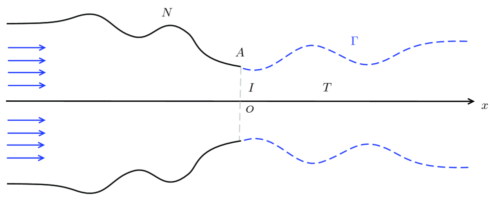
Denote $\displaystyle N=\{y=g(x),x\in(-\infty,0]\}$ the upper nozzle wall of the semi-infinitely long plane symmetric nozzle, which satisfies that

\displaystyle g(x)\in C^{2,\alpha}((-\infty,0])

\displaystyle\lim_{x\rightarrow-\infty}g(x)=H

and

\displaystyle g(0)=a=\min_{x\leq 0}g(x)

(4.1)

Let $\displaystyle T=\{y=0\}$ be the symmetric axis, and $\displaystyle A=(0,a)$ be the end point of the nozzle wall.

The problem of incompressible jet flow with general vorticity can be formulated as the free boundary problem of finding a domain $\displaystyle\Omega_{0}$ in $\displaystyle(x,y)$ -plane, whose boundary consists of the upper nozzle wall $\displaystyle N$ , the symmetric axis $\displaystyle T$ , and a priori unknown curve $\displaystyle\Gamma$ expressed by $\displaystyle y=k(x)$ for $\displaystyle x\geq 0$ with

k(0)=g(0)=a\ \ \ \text{and}\ \ \ k^{\prime}(0)=g^{\prime}(0).

(4.2)

The condition (4.2) is the so-called continuous fit condition and smooth fit condition, respectively.

A vector $\displaystyle(u,v,p)$ representing the horizontal velocity, the vertical velocity and the pressure of the flow in $\displaystyle\Omega_{0}$ , which belongs to $\displaystyle\left(C^{1,\alpha}(\Omega_{0})\cap C^{0}(\bar{\Omega}_{0})\right)^{3}$ and satisfies the steady incompressible Euler equations

\left\{\begin{array}[]{ll}&\partial_{x}u+\partial_{y}v=0,\\ &u\partial_{x}u+v\partial_{y}u+\partial_{x}p=0,\\ &u\partial_{x}v+v\partial_{y}v+\partial_{y}p=0,\end{array}\right.

(4.3)

and the slip boundary condition

(u,v)\cdot\vec{n}=0\ \ \ \text{on}\ \ \ N\cup T,

(4.4)

where $\displaystyle\vec{n}$ is the normal direction of the boundary.

The free boundary $\displaystyle\Gamma$ is assumed to be a material surface of the incompressible fluid, and then the velocity still satisfies the slip boundary condition (4.4) on $\displaystyle\Gamma$ . Moreover, the classical assumption (neglecting the effects of surface tension) is constant pressure condition, namely,

p=p_{atm}\ \ \ \text{on}\ \ \ \Gamma.

Here, we denote $\displaystyle p_{atm}$ the constant atmosphere pressure.

In the upstream, we assume that

u(x,y)\rightarrow u_{0}(y)\ \ \text{and}\ \ v(x,y)\rightarrow 0\ \ \text{as}\ \ x\rightarrow-\infty,

(4.5)

and denote $\displaystyle p_{in}$ the constant champer pressure in the inlet of the nozzle. Here, the variation and amplitude of the horizontal velocity $\displaystyle u_{0}(y)$ are arbitrary, and it implies that the vorticity of the jet flow is arbitrary in the upstream.

Remark 4.1.

Once we impose the horizontal velocity $\displaystyle u_{0}(y)$ in the inlet of the nozzle, the mass flux of incoming flow is determined by

Q=\int_{0}^{H}u_{0}(y)dy.

Before we state the well-posedness results on the incompressible jet problem, it should be noted that there are two invariant quantities for the steady incompressible inviscid fluid, i.e.,

(u,v)\cdot\nabla\omega=0,

(4.6)

and

(u,v)\cdot\nabla\left(\frac{1}{2}(u^{2}+v^{2})+p\right)=0,

(4.7)

where $\displaystyle\omega=v_{x}-u_{y}$ denotes the vorticity of the fluid in two dimensions. In particular, the relation (4.7) gives that quantity $\displaystyle\frac{1}{2}(u^{2}+v^{2})+p$ called Bernoulli’s function remains invariant along the each streamline, which tells us two facts,
(1) the speed remains a constant denoted as $\displaystyle\lambda$ along the free boundary $\displaystyle\Gamma$ .
(2) along the upper nozzle wall and the free boundary $\displaystyle\Gamma$ ,

\lambda=\sqrt{u^{2}_{0}(H)+2(p_{in}-p_{atm})}

as long as the continuous fit condition of the free boundary holds, where $\displaystyle p_{in}$ denotes the uniform pressure in the upstream. Here, the quantity $\displaystyle p_{diff}=p_{in}-p_{atm}$ is nothing but the pressure difference between the upstream and the downstream. It should be noted that the quantity $\displaystyle p_{diff}$ is an undermined parameter here, and we will show that the appropriate choice $\displaystyle p_{diff}$ is guaranteed by the continuous fit condition.

The incompressible jet problem is stated as follows.

The incompressible jet flow problem. Given a symmetric semi-infinitely long nozzle $\displaystyle N$ , a horizontal velocity $\displaystyle u_{0}(y)$ in the inlet and a constant atmosphere pressure $\displaystyle p_{atm}$ on the free surface, does there exist a unique symmetric incompressible inviscid jet flow issuing from the nozzle $\displaystyle N$ , and the free boundary $\displaystyle\Gamma$ initiates smoothly at the endpoint $\displaystyle A$ .

Moreover, we introduce the definition of a solution to the incompressible jet flow problem in the following.

Definition 4.1.

(A solution to the incompressible jet flow problem).
Given an atmosphere pressure $\displaystyle p_{atm}$ and an incoming velocity $\displaystyle u_{0}(y)$ , a vector $\displaystyle(u,v,p,\Gamma)$ is called a solution to the incompressible jet flow problem, provided that
(1) The free boundary $\displaystyle\Gamma$ can be expressed by a $\displaystyle C^{1}$ -smooth function $\displaystyle y=k(x)>0$ for any $\displaystyle x\in[0,+\infty)$ , and there exists an appropriate pressure difference $\displaystyle p_{diff}$ , such that $\displaystyle\Gamma$ satisfies the continuous and smooth fit condition (4.2).
(2) $\displaystyle(u,v,p)\in\left(C^{1,\alpha}(\Omega_{0})\cap C(\bar{\Omega}_{0})\right)^{3}$ solves the Euler system (4.3), and satisfies the boundary condition (4.4).
(3) There exists a unique positive constant $\displaystyle h\in(0,a]$ such that

k(x)\rightarrow h\ \ \text{and}\ \ k^{\prime}(x)\rightarrow 0\ \ \text{as $\displaystyle x\rightarrow+\infty$}.

where $\displaystyle h$ is the asymptotic height of the free boundary in downstream.
(4) $\displaystyle p=p_{atm}$ on $\displaystyle\Gamma$ .
(5) $\displaystyle(u,v)\rightarrow(u_{0}(y),0)$ uniformly for $\displaystyle y\in(0,H)$ , as $\displaystyle x\rightarrow-\infty$ .

The main results on the existence and uniqueness of the incompressible jet flow problem read as follows.

Theorem 4.1.

Suppose that the nozzle wall $\displaystyle N$ satisfies the assumption condition (4.1). Assume that the horizontal velocity in upstream $\displaystyle u_{0}(y)\in C^{2,\beta}([0,H])$ satisfies that

u_{0}(y)>0,\ u_{0}^{\prime}(0)=0,\ \ \text{and}\ \ u_{0}^{\prime\prime}(y)\geq 0\ \ \text{for any $\displaystyle y\in[0,H]$}.

(4.8)

Then, there exist a unique difference pressure $\displaystyle p_{diff}\geq 0$ and a unique solution $\displaystyle(u,v,p,\Gamma)$ to the incompressible jet flow problem, such that
(1) The jet flow satisfies the following asymptotic behavior in the far fields,

(u,v,p)\rightarrow(u_{0}(y),0,p_{in}),\ \nabla u\rightarrow(0,u_{0}^{\prime}(y)),~~\nabla v\rightarrow 0,~~\nabla p\rightarrow 0,

uniformly in any compact subset of $\displaystyle(0,H)$ , as $\displaystyle x\rightarrow-\infty$ , and

(u,v,p)\rightarrow(u_{1}(y),0,p_{atm}),\ \nabla u\rightarrow(0,u_{1}^{\prime}(y)),~~\nabla v\rightarrow 0,~~\nabla p\rightarrow 0,

uniformly in any compact subset of $\displaystyle(0,h)$ , as $\displaystyle x\rightarrow+\infty,$ where $\displaystyle p_{in}=p_{diff}+p_{atm}$ , and $\displaystyle u_{1}(y)$ and $\displaystyle h$ are uniquely determined by $\displaystyle u_{0}(y)$ , $\displaystyle p_{in}$ and $\displaystyle p_{atm}$ .
(2) $\displaystyle u>0$ in $\displaystyle\bar{\Omega}_{0}$ .
(3) $\displaystyle h\leq k(x)\leq\bar{H}=\max_{x\leq 0}g(x)$ for any $\displaystyle x\in[0,\infty)$ .

Remark 4.2.

The assumption $\displaystyle u^{\prime}_{0}(0)=0$ in (4.8) follows from the symmetry of the incompressible jet flow. However, if we consider an asymmetric incompressible jet flow, the condition $\displaystyle u^{\prime}_{0}(0)=0$ can be instead of $\displaystyle u^{\prime}_{0}(H)\geq 0$ .

Remark 4.3.

To obtain the continuous fit condition, we choose the difference pressure $\displaystyle p_{diff}$ as a parameter, and then show that there exists a unique $\displaystyle p_{diff}$ , such that the free boundary $\displaystyle\Gamma$ satisfies the continuous fit condition in (4.2).

Similarly, we can obtain the well-posedness results on the incompressible cavitational flow problem. We will give the statement of the physical problem and the well-posedness results as follows.

Given a two-dimensional obstacle as

N:y=g(x)\in C^{2,\alpha}((-b,0]),\ g(-b)=0\ \text{and $\displaystyle g(0)=a=\max_{-b\leq x\leq 0}g(x)$}.

(4.9)

and denote $\displaystyle T_{0}=\{(x,0)\mid-\infty<x<+\infty\}$ the asymmetric axis and $\displaystyle T_{1}=\{(x,H)\mid-\infty<x<+\infty\}$ (see Figure 6).

The incompressible cavitational flow problem. Given a two-dimensional symmetric obstacle $\displaystyle N$ , atmosphere pressure $\displaystyle p_{atm}$ and the horizontal velocity $\displaystyle u_{0}(y)$ in the upstream, does there exist a unique incompressible symmetric inviscid cavitational flow past the given obstacle, and the free boundary $\displaystyle\Gamma$ initiates smoothly at the corner $\displaystyle A$ of the obstacle?

Definition 4.2.

(A solution to the incompressible cavitational flow problem).
A vector $\displaystyle(u,v,p,\Gamma)$ is called a solution to the incompressible cavitational flow problem, provided that
(1) The free boundary $\displaystyle\Gamma$ can be expressed by a $\displaystyle C^{1}$ -smooth function $\displaystyle y=k(x)>0$ for any $\displaystyle x\in[0,+\infty)$ , such that $\displaystyle N\cup\Gamma$ is $\displaystyle C^{1}$ , namely,

g(0)=k(0)=a~~\text{and}~~g^{\prime}(0)=k^{\prime}(0).

(4.10)

(2) $\displaystyle(u,v,p)\in\left(C^{1,\alpha}(\Omega_{0})\cap C(\bar{\Omega}_{0})\right)^{3}$ solves the Euler system (4.3), and satisfies the boundary condition (4.6), where $\displaystyle\Omega_{0}$ is the flow field bounded by $\displaystyle N,T_{0},T_{1}$ and $\displaystyle\Gamma$ .
(3) There exists a positive constant $\displaystyle h\in(a,H)$ such that

k(x)\rightarrow h\ \ \text{and}\ \ k^{\prime}(x)\rightarrow 0\ \ \text{as}\ \ x\rightarrow+\infty.

We give the results as follows.

Theorem 4.2.

Suppose that the solid wall $\displaystyle N$ satisfies the assumption (4.9). Given an atmosphere pressure $\displaystyle p_{atm}$ and $\displaystyle u_{0}(y)\in C^{2,\beta}([0,H])$ , which satisfies that

u_{0}(y)>0,\ \ u_{0}^{\prime}(0)=0\ \ \text{and}\ \ u_{0}^{\prime\prime}(y)\geq 0\ \ \text{for any $\displaystyle y\in[0,H]$}.

(4.11)

Then, there exist a unique difference pressure $\displaystyle p_{diff}=p_{up}-p_{atm}$ and a unique solution $\displaystyle(u,v,p,\Gamma)$ to the cavitational flow problem, where $\displaystyle p_{in}$ denotes the pressure in the inlet of the channel. Furthermore,
(1) The cavitational flow satisfies the following asymptotic behavior in the far fields,

(u,v,p)\rightarrow(u_{0}(y),0,p_{in}),\ \nabla u\rightarrow(0,u_{0}^{\prime}(y)),~~\nabla v\rightarrow 0,~~\nabla p\rightarrow 0,

uniformly in any compact subset of $\displaystyle(0,H)$ , as $\displaystyle x\rightarrow-\infty$ , and

(u,v,p)\rightarrow(u_{1}(y),0,p_{atm}),\ \nabla u\rightarrow(0,u_{1}^{\prime}(y)),~~\nabla v\rightarrow 0,~~\nabla p\rightarrow 0,

uniformly in any compact subset of $\displaystyle(h,H)$ , as $\displaystyle x\rightarrow+\infty,$ where $\displaystyle u_{1}(y)$ and $\displaystyle h$ are uniquely determined by $\displaystyle u_{0}(y)$ , $\displaystyle p_{in}$ and $\displaystyle p_{atm}$ .
(2) $\displaystyle u>0$ in $\displaystyle\bar{\Omega}_{0}$ .
(3) $\displaystyle k(x)>0$ for any $\displaystyle x>0$ .

4.2. Reformulation of the free boundary problem

In the following, we will reformulate the original physical problem into a free boundary problem of a semilinear elliptic equation. The similar idea has been adapted in the compressible subsonic flows with general vorticity in an infinitely long nozzle in [17, 18, 35].

First, it follows from the continuity equation in the incompressible Euler system (4.3) that there exists a stream function $\displaystyle\psi$ , such that

u=\psi_{y}\ \ ~~\text{and}~~\ \ v=-\psi_{x}.

(4.12)

Second, suppose that the streamlines are well-defined in the whole flow fluid, and thus the incompressible jet flow problem can be solved along the each streamline as follows. On another hand, the positivity of the horizontal velocity of the jet will be verified later, which gives the well-definedness of the streamlines in the whole flow fluid.

Denote $\displaystyle\Omega=\{-\infty<x\leq 0,0<y<g(x)\}\cup\{x>0,y>0\}$ the possible flow field (see Figure 7) and $\displaystyle\Omega_{0}=\Omega\cap\{0<\psi<Q\}$ the flow field. For any point $\displaystyle(x,y)\in\Omega_{0}$ , it can be pulled back along one streamline to the point $\displaystyle(-\infty,\kappa(\psi(x,y)))$ in the inlet. Thus

\psi(x,y)=\int_{0}^{\kappa(\psi(x,y))}u_{0}(s)ds,

which implies that

\left\{\begin{array}[]{ll}&1=u_{0}(\kappa(\psi))\kappa^{\prime}(\psi),\\ &\kappa(0)=0.\end{array}\right.

(4.13)

It’s easy to see that the function $\displaystyle\kappa(t)$ can be solved uniquely by (4.13) provided that $\displaystyle u_{0}(y)$ is $\displaystyle C^{2,\beta}$ -smooth. Meanwhile, it’s clear that $\displaystyle\kappa(Q)=H$ . Due to the fact that the vorticity $\displaystyle\omega$ is invariable on each streamline, we obtain the governing equation to the stream function,

\begin{array}[]{rl}-\Delta\psi=\omega=-u^{\prime}_{0}(\kappa(\psi))\triangleq f_{0}(\psi)\ \ \ \ \text{in the fluid field $\displaystyle\Omega_{0}$}.\end{array}

Furthermore, it is not difficult to check the following facts

\begin{array}[]{rl}&\text{(1) $\displaystyle f_{0}(t)$ is $\displaystyle C^{1,\beta}$,}\\ &\text{(2) $\displaystyle f_{0}(0)=0,f_{0}(Q)=-u_{0}^{\prime}(H)\leq 0$},\\ &\text{(3) $\displaystyle f_{0}^{\prime}(t)=-\frac{u_{0}^{\prime\prime}(\kappa(t))}{u_{0}(\kappa(t))}\leq 0$},\end{array}

(4.14)

provided that $\displaystyle u_{0}(y)$ satisfies the assumption (4.8).

On another hand, we can impose the Dirichlet boundary conditions,

\psi=Q~~\text{on}~~N\cup I_{0},~~\text{and}~\psi=0~\text{on}~T,

where $\displaystyle I_{0}=\{(0,y)\mid y\geq a\}$ . Moreover, the free boundary can be defined as

\Gamma=\Omega\cap\{x>0\}\cap\partial{\{\psi<Q\}}.

(4.15)

The constant pressure condition on the free boundary together with the Bernoulli’s law gives that the speed remains a constant on $\displaystyle\Gamma$ , denote $\displaystyle\lambda$ the constant speed, i.e.,

|\nabla\psi|=\lambda=\sqrt{u^{2}_{0}(H)+2p_{diff}}\ \ \text{on $\displaystyle\Gamma$}.

Clearly, the constant $\displaystyle\lambda$ is determined uniquely by $\displaystyle p_{diff}\geq 0$ .

Therefore, we formulate the following free boundary problem of the stream function that

\left\{\begin{array}[]{ll}&-\Delta\psi=f_{0}(\psi)~~~~\ \ \ \text{in}~~\Omega\cap\{\psi<Q\},\\ &\psi=Q~~~~\ \ \ \text{on}~~N\cup\Gamma,\ \ \ \ \ \psi=0~~~~\text{on}~~T,\\ &|\nabla\psi|=\lambda~~~~\ \ \ \text{on}~~\Gamma.\end{array}\right.

(4.16)

4.3. Uniqueness of asymptotic behavior in downstream

Next, we will show that the asymptotic behavior of the jet flow in downstream can be determined by the state $\displaystyle(u_{0}(y),0)$ of the incoming flow and the difference pressure $\displaystyle p_{diff}$ .

For any initiate point $\displaystyle(-\infty,s)$ in the inlet, the well-definedness of the streamlines implies that there exists a unique point denoted $\displaystyle(0,\chi(s;p_{diff}))$ in the downstream for any $\displaystyle s\in[0,H]$ (see Figure 8), which can be pulled back to the imposed initiate point $\displaystyle(-\infty,s)$ along a streamline.

Denote $\displaystyle u_{1}(y)$ the horizontal velocity in the downstream, the conservation of mass and Bernoulli’s law gives that

\int_{0}^{s}u_{0}(t)dt=\int_{0}^{\chi(s;p_{diff})}u_{1}(t)dt,

and

\frac{u^{2}_{0}(s)}{2}+p_{diff}=\frac{u^{2}_{1}(\chi(s;p_{diff}))}{2}\ \ \text{in the fluid field}.

Here, the difference pressure $\displaystyle p_{diff}\geq 0$ between the inlet and the downstream is regarded as a parameter. These also give the initial value problem to the function $\displaystyle\chi(s;p_{diff})$ as follows,

\left\{\begin{array}[]{ll}&\frac{d\chi(s;p_{diff})}{ds}=\frac{u_{0}(s)}{\sqrt{u_{0}^{2}(s)+2p_{diff}}}>0,\\ &\chi(0;p_{diff})=0,\end{array}\right.

(4.17)

for any $\displaystyle s\in[0,H]$ and $\displaystyle p_{diff}\geq 0$ . Thus,

\chi(s;p_{diff})=\int_{0}^{s}\frac{u_{0}(t)}{\sqrt{u_{0}^{2}(t)+2p_{diff}}}dt\leq s.

(4.18)

It is easy to check that $\displaystyle\chi(s;p_{diff})$ is strictly decreasing with respect to the parameter $\displaystyle p_{diff}$ . In particular, the asymptotic height of the jet in downstream is in fact $\displaystyle h=\chi(H;p_{diff})$ .

Noting that $\displaystyle\frac{d\chi(s;p_{diff})}{ds}>0$ for any $\displaystyle s\in[0,H]$ and $\displaystyle p_{diff}\geq 0$ , thus there exists an inverse function $\displaystyle\chi^{-1}(t;p_{diff})$ , such that $\displaystyle s=\chi^{-1}(t;p_{diff})$ for any $\displaystyle t\in[0,h]$ . Then the horizontal velocity $\displaystyle u_{1}(y)$ in downstream can be solved uniquely by

u_{1}(t)=\sqrt{u_{0}^{2}(\chi^{-1}(t;p_{diff}))+2p_{diff}}\ \ \text{for any $\displaystyle t\in[0,h]$},

(4.19)

once $\displaystyle\chi(s;p_{diff})$ is solved by the initiate value problem (4.17) for any $\displaystyle p_{diff}\geq 0$ .

Remark 4.4.

For any $\displaystyle p_{diff}\geq 0$ , it is easy to check that

\text{$\displaystyle\frac{d\chi(H;p_{diff})}{dp_{diff}}<0$ and}\ \ \lambda=\sqrt{u^{2}_{0}(H)+2p_{diff}}\geq u_{0}(H)\triangleq\lambda_{0}\geq 0.

Moreover, the asymptotic height $\displaystyle h=\chi(H;p_{diff})=\chi\left(H;\frac{\lambda^{2}-u^{2}_{0}(H)}{2}\right)=h(\lambda)\triangleq h_{\lambda}$ is strictly increasing with respect to $\displaystyle\lambda$ , and $\displaystyle h_{\lambda_{0}}=H$ .

4.4. The variational approach

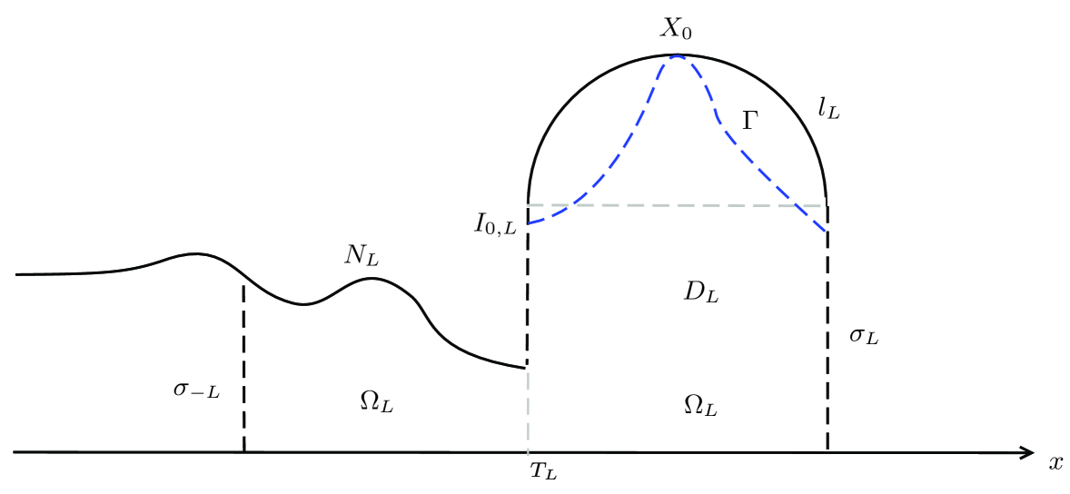
To solve the free boundary problem (4.16), we introduce a variational problem with a parameter $\displaystyle\lambda\geq\lambda_{0}$ . For any $\displaystyle L>\bar{H}=\max_{x\leq 0}g(x)$ , denote $\displaystyle\Omega_{L}$ the truncated domain (see Figure 9),

\Omega_{L}=\Omega\cap\{(x,y)\mid-L<x<L,y<L\},\ \ \ \ D_{L}=\Omega_{L}\cap\{x>0\},\ \ \ N_{L}=N\cap\{x>-L\},

and

\sigma_{-L}=\{(-L,y)|~0\leq y\leq g(-L)\}\ \ \ \text{and}\ \ \ \ \sigma_{L}=\{(L,y)|~0\leq y\leq L\},

and

T_{L}=T\cap\{-L\leq x\leq L\},\ I_{0,L}=\{(0,y)\mid a\leq y\leq L\}\ \ \text{and}\ \ l_{L}=\partial B_{L/2}\left(\left(L/2,L\right)\right)\cap\{y\geq L\}.

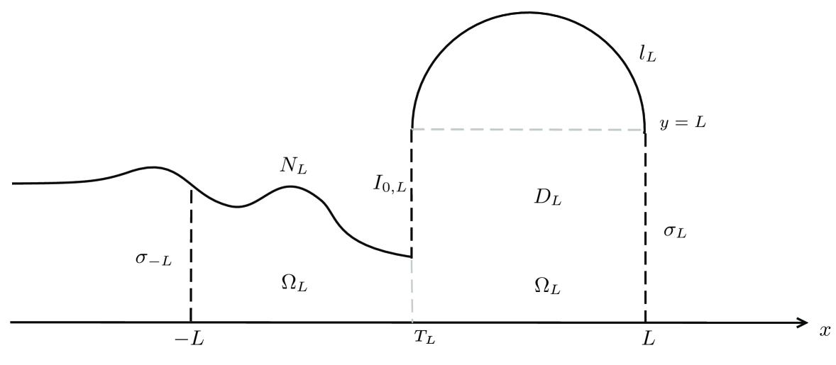
Since, a priorily, one does not know whether the stream function $\displaystyle\psi$ satisfies that $\displaystyle 0\leq\psi\leq Q$ . Hence, we need extend the function $\displaystyle f_{0}(t)$ as follows

\tilde{f}_{0}(t)=\left\{\begin{array}[]{ll}f_{0}(Q)+\frac{f_{0}^{\prime}(Q)}{2}&\text{if}~~t\geq Q+1,\\ f_{0}(Q)+f_{0}^{\prime}(Q)\left(t-Q-\frac{(t-Q)^{2}}{2}\right)&\text{if}~~Q\leq t\leq Q+1,\\ f_{0}(t)&\text{if}~~0\leq t\leq Q,\\ f_{0}^{\prime}(0)\left(t+\frac{t^{2}}{2}\right)&\text{if}~~-1\leq t\leq 0,\\ -\frac{f_{0}^{\prime}(0)}{2}&\text{if}~~t\leq-1.\end{array}\right.

(4.20)

Set

\text{$\displaystyle F_{0}(t)=2\int_{t}^{Q}\tilde{f}_{0}(t)ds$\ \ \ and \ \ \ $\displaystyle f(t)=-\tilde{f}_{0}(Q-t)$}.

(4.21)

For $\displaystyle y\in[0,g(-L)]$ , define a function $\displaystyle\Psi_{-L}(y)$ , which satisfies that

\Psi_{-L}^{\prime\prime}(y)=-\tilde{f}_{0}(\Psi_{-L}(y)),\ \Psi_{-L}(0)=0,\ \Psi_{-L}(g(-L))=Q.

By virtue of (4.14), it is easy to check that

0<\Psi_{-L}(y)<Q\ \ \text{and}\ \ \Psi^{\prime}_{-L}(y)\geq 0\ \ \text{for any $\displaystyle y\in(0,g(-L))$.}

Firstly, we give the following functional that

J_{\lambda,L}(\psi)=\int_{\Omega_{L}}\left(|\nabla\psi|^{2}+F_{0}(\psi)+\lambda^{2}I_{\{\psi<Q\}\cap D_{L}}\right)dX,

where the admissible set is defined as follows

\begin{array}[]{rl}K_{\lambda,L}=\{\psi\in H^{1}_{loc}(\mathbb{R}^{2})\mid&\psi=0~~\text{lies below}~T,\psi=Q~~\text{lies above}~N\cup I_{0,L}\cup l_{L},\\ &\psi=\Psi_{-L}~~~\text{on}~~\sigma_{-L},~~~\psi=\min\{\Psi_{\lambda},Q\}~~~\text{on}~~\sigma_{L}\},\end{array}

and

\Psi_{\lambda}(y)=\int_{0}^{y}u_{1}(s)ds.

(4.22)

Truncated variational problem $\displaystyle(P_{\lambda,L})$ : For any $\displaystyle L>\bar{H}$ and $\displaystyle\lambda\geq\lambda_{0}$ , find a $\displaystyle\psi_{\lambda,L}\in K_{\lambda,L}$ such that

J_{\lambda,L}(\psi_{\lambda,L})=\min_{\psi\in K_{\lambda,L}}J_{\lambda,L}(\psi).

Remark 4.5.

Set $\displaystyle\phi=Q-\psi$ , by virtue of (4.14) and (4.21), the variational problem $\displaystyle(P_{\lambda,L})$ can be transformed into the variational problem in Section 2, and $\displaystyle f(t)$ satisfies the condition (2.1). Thus, we can use the results in Section 2 and Section 3 in the following.

Proposition 4.3.

For any $\displaystyle\lambda\geq\lambda_{0}$ and $\displaystyle L>\bar{H}$ , there exists a minimizer $\displaystyle\psi_{\lambda,L}$ to the variational problem $\displaystyle(P_{\lambda,L})$ with $\displaystyle 0\leq\psi_{\lambda,L}(x,y)\leq Q$ in $\displaystyle\Omega_{L}$ .

Proof.

The existence of the minimizer to the variational problem $\displaystyle P_{\lambda,L}$ follows from Lemma 2.1, and denote $\displaystyle\psi_{\lambda,L}$ the minimizer to the variational problem $\displaystyle(P_{\lambda,L})$ .

Denote $\displaystyle\psi=\psi_{\lambda,L}$ and $\displaystyle\psi^{\varepsilon}=\psi-\varepsilon\min\{\psi,0\}$ for any $\displaystyle\varepsilon\in(0,1)$ . Thus, $\displaystyle\psi^{\varepsilon}\in K_{\lambda,L}$ and $\displaystyle\psi^{\varepsilon}\geq\psi$ . Moreover, $\displaystyle\psi<Q$ if and only if $\displaystyle\psi^{\varepsilon}<Q$ in $\displaystyle\Omega_{L}$ , and we have

\begin{array}[]{rl}0\leq&J_{\lambda,L}(\psi^{\varepsilon})-J_{\lambda,L}(\psi)\\ \leq&\int_{\Omega_{L}\cap\{\psi<0\}}((1-\varepsilon)^{2}-1)|\nabla\psi|^{2}-\varepsilon F^{\prime}_{0}((1-\varepsilon)\psi)\psi dX\\ \leq&0,\end{array}

due to $\displaystyle F^{\prime}(t)\leq 0$ for $\displaystyle t\leq 0$ , which implies that

\text{$\displaystyle\psi(x,y)\geq 0$ in $\displaystyle\Omega_{L}$}.

Similarly, we can show that

\text{$\displaystyle\psi(x,y)\leq Q$ in $\displaystyle\Omega_{L}$}.

∎

Since $\displaystyle 0\leq\psi_{\lambda,L}\leq Q$ in $\displaystyle\Omega_{L}$ , we can remove the truncation of the function $\displaystyle\tilde{f}_{0}(t)$ in (4.20). Denote the free boundary of $\displaystyle\psi_{\lambda,L}$ as

\Gamma_{\lambda,L}=D_{L}\cap\partial\{\psi_{\lambda,L}<Q\}.

With the aid of Lemma 2.1 and Theorem 3.15, we have

Proposition 4.4.

The minimizer $\displaystyle\psi_{\lambda,L}$ satisfies that
(1) $\displaystyle\psi_{\lambda,L}\in C^{0,1}(\Omega_{L})$ .
(2) $\displaystyle\Delta\psi_{\lambda,L}+f_{0}(\psi_{\lambda,L})=0$ in $\displaystyle\Omega_{L}\cap\{\psi_{\lambda,L}<Q\}$ and $\displaystyle\Delta\psi_{\lambda,L}+f_{0}(\psi_{\lambda,L})\leq 0$ in $\displaystyle\Omega_{L}$ in the weak sense. Furthermore, $\displaystyle\psi_{\lambda,L}>0$ in $\displaystyle\Omega_{L}$ and $\displaystyle\psi_{\lambda,L}\in C^{2,\alpha}(G)$ for any compact subset $\displaystyle G$ of $\displaystyle\Omega_{L}\cap\{\psi_{\lambda,L}<Q\}$ , $\displaystyle\alpha\in(0,1)$ .
(3) The free boundary of the minimizer $\displaystyle\psi_{\lambda,L}$ is $\displaystyle C^{3,\alpha}$ .
(4) $\displaystyle|\nabla\psi_{\lambda,L}|=\lambda$ on the free boundary $\displaystyle\Gamma_{\lambda,L}$ . Moreover, $\displaystyle|\nabla\psi_{\lambda,L}|\geq\lambda$ on the segment $\displaystyle l\in I_{0,L}\cap\partial\{\psi_{\lambda,L}<Q\}$ and $\displaystyle|\nabla\psi_{\lambda,L}|\leq\lambda$ on the segment $\displaystyle l\in\{x=0,0<y<a\}\cap\partial\{\psi_{\lambda,L}<Q\}$ .

The Statement (1) in Proposition 4.4 gives the Lipschitz continuity of the minimizer in the interior of $\displaystyle\Omega_{L}$ . Next, we will show that the minimizer $\displaystyle\psi_{\lambda,L}(x,y)$ is also Lipschitz continuous near the boundary of $\displaystyle\Omega_{L}$ .

Lemma 4.5.

$\displaystyle\psi_{\lambda,L}(x,y)$ is Lipschitz continuous in every compact subsect of $\displaystyle\bar{\Omega}_{L}$ that does not contain the point $\displaystyle A$ .

Proof.

We first consider the Lipschitz continuity of $\displaystyle\psi_{\lambda,L}$ near the boundary $\displaystyle\partial D_{L}$ . Denote $\displaystyle\phi(X)=Q-\psi_{\lambda,L}(X)$ and $\displaystyle d(X)=\text{dist}(X,\Gamma_{\lambda,L})$ and $\displaystyle d_{1}(X)=\text{dist}(X,\partial D_{L})$ for any $\displaystyle X\in D_{L}$ . We consider the following two cases.

Case 1. $\displaystyle d(X)\leq d_{1}(X)$ , we can obtain the Lipschitz continuity of $\displaystyle\phi$ at $\displaystyle X$ by using the similar arguments in the proof Theorem 2.4.

Case 2. $\displaystyle d(X)>d_{1}(X)$ . Without loss of generality, we assume that $\displaystyle d_{1}(X)=|X-X_{0}|$ for $\displaystyle X_{0}=(0,y)\in I_{0,L}$ and $\displaystyle X=(x,y)\in D_{L}$ . Set $\displaystyle s_{0}=\min\left\{\frac{1}{2},y-a\right\}$ and $\displaystyle B_{s_{0}}=B_{s_{0}}(X_{0})$ . Let $\displaystyle\varphi$ be a solution to the following boundary problem,

\left\{\begin{array}[]{ll}&\Delta\varphi+f(\varphi)=0\ \ \text{in}\ B_{s_{0}}\cap\{x>0\},\\ &\varphi=0\ \text{on}\ B_{s_{0}}\cap\{x=0\},\ \ \varphi=Q\ \text{on}\ \partial B_{s_{0}}\cap\{x>0\}.\end{array}\right.

Since $\displaystyle\phi\leq\varphi$ on $\displaystyle\partial(B_{s_{0}}\cap\{x>0\})$ , the maximum principle gives that

\phi\leq\varphi\ \ \text{in $\displaystyle B_{s_{0}}\cap\{x>0\}$}.

Denote $\displaystyle\tilde{\varphi}(\tilde{X})=\varphi(X_{0}+s_{0}\tilde{X})$ for $\displaystyle\tilde{X}=(\tilde{x},\tilde{y})$ , and $\displaystyle\Delta\tilde{\varphi}+s_{0}^{2}f(\tilde{\varphi})=0$ in $\displaystyle B_{1}(0)\cap\{\tilde{x}>0\}$ . By using the elliptic estimates in [26], we have

\tilde{\varphi}(\tilde{X})\leq C\tilde{x}\ \ \text{in $\displaystyle B_{\frac{1}{2}}(0)\cap\{\tilde{x}>0\}$},

which implies that

\phi(X)\leq\varphi(X)\leq C\frac{x}{s_{0}}\ \ \text{in $\displaystyle B_{\frac{s_{0}}{2}}(X_{0})\cap\{x>0\}$}.

(4.23)

If $\displaystyle r=x<\frac{s_{0}}{4}$ , we have

\phi>0\ \ \text{and}\ \ \Delta\phi+f(\phi)=0\ \ \text{ in $\displaystyle B_{r}(X)\subset B_{\frac{s_{0}}{2}}\cap\{x>0\}$}.

Denote $\displaystyle\tilde{\phi}(\tilde{X})=\frac{\phi(X+r\tilde{X})}{r}$ for $\displaystyle\tilde{X}=(\tilde{x},\tilde{y})$ , it follows from (4.23) that

0<\tilde{\phi}<\frac{C}{s_{0}}\ \ \text{and}\ \ \Delta\tilde{\phi}+rf(r\tilde{\phi})=0\ \ \text{ in $\displaystyle B_{1}(0)$}.

By using the elliptic estimates in [26], we have

|\nabla\phi(X)|=|\nabla\tilde{\phi}(0)|\leq C(\|\tilde{\phi}\|_{L^{\infty}(B_{1}(0))}+r\|f(r\tilde{\phi})\|_{L^{\infty}(B_{1}(0))})\leq\frac{C}{s_{0}}+Cs_{0}.

If $\displaystyle r=x\geq\frac{s_{0}}{4}$ , the elliptic estimate in [26] gives that $\displaystyle|\nabla\phi(X)|\leq C$ .

Since $\displaystyle\Delta\psi_{\lambda,L}+f_{0}(\psi_{\lambda,L})=0$ in $\displaystyle\Omega_{L}\setminus D_{L}$ , the Lipschitz continuity of $\displaystyle\psi_{\lambda,L}$ near $\displaystyle\partial(\Omega_{L}\setminus D_{L})$ can be obtained by using elliptic regularity.

∎

4.5. The uniqueness, monotonicity and free boundary of the minimizer

We first give the uniqueness of the minimizer $\displaystyle\psi_{\lambda,L}(x,y)$ for any given $\displaystyle\lambda\geq\lambda_{0}$ and $\displaystyle L>\bar{H}$ , and show that $\displaystyle\psi_{\lambda,L}(x,y)$ is monotone increasing with respect to $\displaystyle y$ .

Once we have the regularity of the free boundary $\displaystyle\Gamma_{\lambda,L}$ at hand, we will establish some topological properties of the free boundary, provided that some special geometric conditions on the solid boundaries are assumed. For example, it’s desired that the free boundary is $\displaystyle x$ -graph, as long as we assume that the nozzle wall $\displaystyle N$ is a $\displaystyle x$ -graph and the horizontal velocity of the incoming flow is positive.

To obtain this topological property of the free boundary, we will establish the monotonicity of the minimizer $\displaystyle\psi_{\lambda,L}(x,y)$ with respect to $\displaystyle y$ first.

Lemma 4.6.

The minimizer of the truncated variational problem $\displaystyle(P_{\lambda,L})$ is unique and $\displaystyle\psi_{\lambda,L}(x,y)$ is monotone increasing with respect to $\displaystyle y$ .

Proof.

Assume that $\displaystyle\psi_{\lambda,L}$ and $\displaystyle\tilde{\psi}_{\lambda,L}$ are two minimizers to the truncated variational problem $\displaystyle(P_{\lambda,L})$ . Set $\displaystyle\psi_{\lambda,L}^{\varepsilon}(x,y)=\psi_{\lambda,L}(x,y-\varepsilon)$ in $\displaystyle\Omega_{L}^{\varepsilon}=\{(x,y)\mid(x,y-\varepsilon)\in\Omega_{L}\}$ for any $\displaystyle\varepsilon>0$ .

Noticing that $\displaystyle\psi_{\lambda,L}^{\varepsilon}$ is a minimizer to the functional

J_{\lambda,L}^{\varepsilon}(\psi)=\int_{\Omega^{\varepsilon}_{L}}\left(|\nabla\psi|^{2}+F_{0}(\psi)+\lambda^{2}I_{\{\psi<Q\}\cap D^{\varepsilon}_{L}}\right)dX

and the admissible set $\displaystyle K^{\varepsilon}_{\lambda,L}=\{\psi\mid\psi(x,y-\varepsilon)\in K_{\lambda,L}\}$ , where $\displaystyle D_{L}^{\varepsilon}=\Omega_{L}^{\varepsilon}\cap\{x>0\}$ . Extend $\displaystyle\psi_{\lambda,L}^{\varepsilon}=0$ in $\displaystyle\Omega_{L}\setminus\Omega^{\varepsilon}_{L}$ and $\displaystyle\tilde{\psi}_{\lambda,L}=Q$ in $\displaystyle\Omega^{\varepsilon}_{L}\setminus\Omega_{L}$ .

Denote $\displaystyle\tilde{\psi}=\tilde{\psi}_{\lambda,L}$ and $\displaystyle\psi^{\varepsilon}=\psi_{\lambda,L}^{\varepsilon}$ for simplicity, it follows from Proposition 4.3 that

\phi_{1}=\min\{\psi^{\varepsilon},\tilde{\psi}\}\in K^{\varepsilon}_{\lambda,L}\ \ \text{and}\ \ \phi_{2}=\max\{\psi^{\varepsilon},\tilde{\psi}\}\in K_{\lambda,L},

and

\Omega_{L}\cap\{\psi^{\varepsilon}>\tilde{\psi}\}=\Omega_{L}^{\varepsilon}\cap\{\psi^{\varepsilon}>\tilde{\psi}\}.

(4.24)

Next, we will show that

J_{\lambda,L}^{\varepsilon}(\phi_{1})=J_{\lambda,L}^{\varepsilon}(\psi^{\varepsilon})\ \ \text{and}\ \ J_{\lambda,L}(\phi_{2})=J_{\lambda,L}(\tilde{\psi}).

(4.25)

Since $\displaystyle\tilde{\psi}$ and $\displaystyle\psi^{\varepsilon}$ are minimizers, it suffices to show that

J_{\lambda,L}^{\varepsilon}(\phi_{1})+J_{\lambda,L}(\phi_{2})=J_{\lambda,L}(\tilde{\psi})+J_{\lambda,L}^{\varepsilon}(\psi^{\varepsilon}).

(4.26)

It follows from (4.24) that

\begin{array}[]{rl}&\int_{\Omega_{L}^{\varepsilon}}|\nabla\phi_{1}|^{2}dX+\int_{\Omega_{L}}|\nabla\phi_{2}|^{2}dX\\ =&\int_{\Omega_{L}^{\varepsilon}\cap\{\psi^{\varepsilon}\leq\tilde{\psi}\}}|\nabla\psi^{\varepsilon}|^{2}dX+\int_{\Omega_{L}^{\varepsilon}\cap\{\psi^{\varepsilon}>\tilde{\psi}\}}|\nabla\tilde{\psi}|^{2}dX\\ &+\int_{\Omega_{L}\cap\{\psi^{\varepsilon}\leq\tilde{\psi}\}}|\nabla\tilde{\psi}|^{2}dX+\int_{\Omega_{L}\cap\{\psi^{\varepsilon}>\tilde{\psi}\}}|\nabla\psi^{\varepsilon}|^{2}dX\\ =&\int_{\Omega_{L}^{\varepsilon}\cap\{\psi^{\varepsilon}\leq\tilde{\psi}\}}|\nabla\psi^{\varepsilon}|^{2}dX+\int_{\Omega_{L}\cap\{\psi^{\varepsilon}>\tilde{\psi}\}}|\nabla\tilde{\psi}|^{2}dX\\ &+\int_{\Omega_{L}\cap\{\psi^{\varepsilon}\leq\tilde{\psi}\}}|\nabla\tilde{\psi}|^{2}dX+\int_{\Omega_{L}^{\varepsilon}\cap\{\psi^{\varepsilon}>\tilde{\psi}\}}|\nabla\psi^{\varepsilon}|^{2}dX\\ =&\int_{\Omega_{L}}|\nabla\tilde{\psi}|^{2}dX+\int_{\Omega_{L}^{\varepsilon}}|\nabla\psi^{\varepsilon}|^{2}dX.\end{array}

(4.27)

Similarly, we can verify that

\int_{\Omega_{L}^{\varepsilon}}F_{0}(\phi_{1})dX+\int_{\Omega_{L}}F_{0}(\phi_{2})dX=\int_{\Omega_{L}^{\varepsilon}}F_{0}(\psi^{\varepsilon})dX+\int_{\Omega_{L}}F_{0}(\tilde{\psi})dX,

and

\begin{array}[]{rl}\int_{D_{L}^{\varepsilon}}I_{\{\phi_{1}<Q\}}dX+\int_{D_{L}}I_{\{\phi_{2}<Q\}}dX=\int_{D_{L}^{\varepsilon}}I_{\{\psi^{\varepsilon}<Q\}}dX+\int_{D_{L}}I_{\{\tilde{\psi}<Q\}}dX,\end{array}

which together with (4.27) yield (4.26).

Next, we claim that

\text{if $\displaystyle\psi^{\varepsilon}(X_{0})=\tilde{\psi}(X_{0})<Q$ for $\displaystyle X_{0}\in\Omega_{L}$, then either $\displaystyle\psi^{\varepsilon}\geq\tilde{\psi}$ or $\displaystyle\psi^{\varepsilon}\leq\tilde{\psi}$ in $\displaystyle B_{r}(X_{0})$},

(4.28)

for small $\displaystyle r>0$ . Suppose that the claim (4.28) is not true, the continuity of $\displaystyle\tilde{\psi}$ and $\displaystyle\psi^{\varepsilon}$ give that $\displaystyle 0<\tilde{\psi}<Q$ and $\displaystyle 0<\psi^{\varepsilon}<Q$ in $\displaystyle B_{r}(X_{0})$ for small $\displaystyle r>0$ , then we have that $\displaystyle\phi_{2}$ is not a solution of $\displaystyle\Delta\phi_{2}+f_{0}(\phi_{2})=0$ in $\displaystyle B_{r}(X_{0})$ . In fact, if not, the maximum principle gives that $\displaystyle\max\{\tilde{\psi},\psi^{\varepsilon}\}=\phi_{2}=\tilde{\psi}$ in $\displaystyle B_{r}(X_{0})$ , due to $\displaystyle\phi_{2}(X_{0})=\tilde{\psi}(X_{0})$ . This contradicts to our assumptions.

Let $\displaystyle\phi$ be the solution of the following boundary value problem

\left\{\begin{array}[]{ll}\Delta\phi+f_{0}(\phi)=0&\text{in}\ B_{r}(X_{0}),\\ \phi=\phi_{2}&\text{on}\ \partial B_{r}(X_{0}).\end{array}\right.

Thus $\displaystyle\phi\neq\phi_{2}$ in $\displaystyle B_{r}(X_{0})$ , it is easy to check that

\begin{array}[]{rl}&\int_{B_{r}(X_{0})}|\nabla\phi|^{2}+F_{0}(\phi)dX-\int_{B_{r}(X_{0})}|\nabla\phi_{2}|^{2}+F_{0}(\phi_{2})dX\\ \leq&-\int_{B_{r}(X_{0})}|\nabla(\phi-\phi_{2})|^{2}dX<0.\end{array}

(4.29)

Extend $\displaystyle\phi=\phi_{2}$ in $\displaystyle\Omega_{L}\setminus B_{r}(X_{0})$ , it follows from (4.25) and (4.29) that

J_{\lambda,L}(\phi)<J_{\lambda,L}(\phi_{2})=J_{\lambda,L}(\tilde{\psi}),

which contradicts to the minimality of $\displaystyle\tilde{\psi}$ .

Since $\displaystyle\tilde{\psi}>\psi^{\varepsilon}$ near $\displaystyle T_{L}$ , it follows from (4.28) that $\displaystyle\tilde{\psi}\geq\psi^{\varepsilon}$ in the connected component $\displaystyle\Omega_{0}$ of $\displaystyle\{\tilde{\psi}<Q\}$ which contains an $\displaystyle\Omega_{L}$ -neighborhood of $\displaystyle T_{L}$ . In view of the boundary value of $\displaystyle\tilde{\psi}$ , we have that $\displaystyle\{\tilde{\psi}<Q\}\cap\partial\Omega_{L}$ is a connected arc. The maximum principle gives that any component of $\displaystyle\{\tilde{\psi}<Q\}$ must touch the boundary $\displaystyle\{\tilde{\psi}<Q\}\cap\partial\Omega_{L}$ . Therefore, the domain $\displaystyle\Omega_{L}\cap\{\tilde{\psi}<Q\}$ is connected and

\psi(x,y-\varepsilon)=\psi^{\varepsilon}(x,y)\leq\tilde{\psi}(x,y)\ \text{in}~~\Omega_{L}.

(4.30)

Similarly, we can show that

\psi(x,y+\varepsilon)\geq\tilde{\psi}(x,y)~~\text{in}~~\Omega_{L}.

(4.31)

Taking $\displaystyle\varepsilon\rightarrow 0$ in (4.30) and (4.31), which yields that

\psi(x,y)=\tilde{\psi}(x,y)~~\text{in}~~\Omega_{L}.

In particular, taking $\displaystyle\psi=\tilde{\psi}$ in (4.30), we have that the minimizer $\displaystyle\psi=\psi_{\lambda,L}(x,y)$ is monotone increasing with respect to $\displaystyle y$ .

∎

The monotonicity of $\displaystyle\psi_{\lambda,L}(x,y)$ with respect to $\displaystyle y$ implies that the free boundary $\displaystyle\Gamma_{\lambda}$ is a $\displaystyle x$ -graph, and then there exists a function $\displaystyle y=k_{\lambda,L}(x)$ for $\displaystyle x\in(0,L)$ , such that

\{\psi_{\lambda,L}<Q\}\cap D_{L}=\{(x,y)\in D_{L}\mid 0<y<k_{\lambda,L}(x),0<x<L\}.

To obtain the continuity of $\displaystyle k_{\lambda,L}(x)$ , we first give the following non-oscillation lemma.

Lemma 4.7.

(Non-oscillation Lemma) Suppose that there exist some constants $\displaystyle\alpha_{1},\alpha_{2}$ with $\displaystyle\alpha_{1}<\alpha_{2}$ and a domain $\displaystyle D\subset D_{L}\cap\{\psi_{\lambda,L}<Q\}$ with dist $\displaystyle(A,D)>c_{0}$ for some $\displaystyle c_{0}>0$ , which is bounded by two disjointed arcs $\displaystyle\gamma_{1},\gamma_{2}$ ( $\displaystyle\gamma_{1},\gamma_{2}\subset\Gamma_{\lambda,L})$ , the lines $\displaystyle\{y=\alpha_{1}\}$ and $\displaystyle\{y=\alpha_{2}\}$ . Denote $\displaystyle(\beta_{i},\alpha_{1})$ and $\displaystyle(\eta_{i},\alpha_{2})$ the endpoints of $\displaystyle\gamma_{i}$ for $\displaystyle i=1,2$ . Then there exists a constant $\displaystyle C>0$ , such that

\alpha_{2}-\alpha_{1}\leq C\max\{|\beta_{1}-\beta_{2}|,|\eta_{1}-\eta_{2}|\}.

Proof.

Denote $\displaystyle h=\max\left\{|\beta_{1}-\beta_{2}|,|\eta_{1}-\eta_{2}|\right\}$ and $\displaystyle\psi=\psi_{\lambda,L}$ . Since $\displaystyle\Delta\psi=-f_{0}(\psi)$ in $\displaystyle D$ , we have

\int_{\partial D}\frac{\partial\psi}{\partial\nu}dS=-\int_{D}f_{0}(\psi)dX\leq\int_{D}-f_{0}(Q)+CQdX\leq Ch(\alpha_{2}-\alpha_{1})\leq Ch,

which implies that

\int_{\gamma_{1}\cup\gamma_{2}}\lambda dS=\int_{\gamma_{1}\cup\gamma_{2}}\frac{\partial\psi}{\partial\nu}dS\leq\int_{\partial D\cap(\{y=\alpha_{1}\}\cup\{y=\alpha_{2}\})}\left|\frac{\partial\psi}{\partial x}\right|dy+Ch\leq Ch,

(4.32)

where we have used the Lipschitz continuity of $\displaystyle\psi$ due to Lemma 4.5.

On the other hand, one gets

\int_{\gamma_{1}\cup\gamma_{2}}\lambda dS\geq 2\lambda(\alpha_{2}-\alpha_{1}),

which together with (4.32) gives that

\alpha_{2}-\alpha_{1}\leq Ch.

∎

With the aid of Lemma 4.7, we have

Lemma 4.8.

$\displaystyle k_{\lambda,L}(x)$ is a continuous function in $\displaystyle[0,L]$ .

Proof.

By using the non-oscillation Lemma 4.7, it follows from the similar arguments in Lemma 5.4 in [5] that $\displaystyle k_{\lambda,L}(x)$ has at most one limit point as $\displaystyle x\downarrow 0$ and $\displaystyle x\uparrow L$ . Moreover, $\displaystyle k_{\lambda,L}(x)$ has most one limit point as $\displaystyle x\uparrow x_{0}$ or as $\displaystyle x\downarrow x_{0}$ for any $\displaystyle x_{0}\in(0,L)$ . It suffices to show that

k_{\lambda,L}(x+0)=k_{\lambda,L}(x-0)=k_{\lambda,L}(x)\ \ \text{for any $\displaystyle x\in(0,L)$}.

If not, without loss of generality, we assume that there exists a point $\displaystyle x_{0}\in(0,L)$ , such that $\displaystyle k_{\lambda,L}(x_{0})<k_{\lambda,L}(x_{0}+0)$ . Denote $\displaystyle I_{\delta}=\{(x_{0},y)\mid k_{\lambda,L}(x_{0})+\delta<y<k_{\lambda,L}(x_{0})+3\delta\}$ with $\displaystyle\delta=\frac{k_{\lambda,L}(x_{0}+0)-k_{\lambda,L}(x_{0})}{4}$ . The monotonicity of $\displaystyle\psi_{\lambda,L}(x,y)$ with respect to $\displaystyle y$ and the Lipschitz continuity of $\displaystyle\psi_{\lambda,L}(x,y)$ give that

\psi_{\lambda,L}=Q\ \ \text{on}\ I_{\delta},\ \ \text{$\displaystyle\Delta\psi_{\lambda,L}+f_{0}(\psi_{\lambda,L})=0$ and $\displaystyle u=\frac{\partial\psi_{\lambda,L}}{\partial y}\geq 0$ in $\displaystyle E_{\delta,\varepsilon}$,}

where $\displaystyle E_{\delta,\varepsilon}=\{(x,y)\mid x_{0}<x<x_{0}+\varepsilon,k_{\lambda,L}(x_{0})+\delta<y<k_{\lambda,L}(x_{0})+3\delta\}$ for small $\displaystyle\varepsilon>0$ . Thus, $\displaystyle I_{\delta}$ is a part of the free boundary $\displaystyle\Gamma_{\lambda,L}$ , it follows from (4) in Proposition 4.4 that

\frac{\partial\psi_{\lambda,L}(x_{0}+0,y)}{\partial x}=|\nabla\psi_{\lambda,L}|=\lambda\ \ \text{on}\ \ I_{\delta}.

(4.33)

It is easy to check that

\Delta u+b(X)u=0\ \ \text{in}\ \ E_{\delta,\varepsilon}\ \ \text{and}\ \ b(X)=f^{\prime}_{0}(\psi_{\lambda,L}(X))\leq 0.

The strong maximum principle gives that $\displaystyle u>0$ in $\displaystyle E_{\delta,\varepsilon}$ . In view of $\displaystyle u=0$ on $\displaystyle I_{\delta}$ , thanks to Hopf’s lemma, we have

\frac{\partial^{2}\psi_{\lambda,L}}{\partial x\partial y}=\frac{\partial u}{\partial x}>0\ \ \text{on}\ \ I_{\delta}.

(4.34)

On the other hand, it follows from (4.33) that

\frac{\partial^{2}\psi_{\lambda,L}}{\partial y\partial x}=0\ \ \text{on}\ \ I_{\delta},

which contradicts to (4.34).

Hence, we obtain the continuity of the function $\displaystyle k_{\lambda,L}(x)$ .

∎

Next, we will introduce the bounded gradient lemma for $\displaystyle\psi_{\lambda,L}$ near the boundary of $\displaystyle D_{L}$ .

Lemma 4.9.

For any $\displaystyle X_{0}\in\partial D_{L}$ , if $\displaystyle B_{R}(X_{0})\cap\Gamma_{\lambda,L}\neq\varnothing$ for any $\displaystyle R>0$ , then for small $\displaystyle r>0$ , there exists a constant $\displaystyle C$ independent of $\displaystyle Q$ and $\displaystyle r$ , such that

|\nabla\psi_{\lambda,L}(X)|\leq C\ \ \text{in $\displaystyle B_{r}(X_{0})\cap\Omega_{L}$}.

(4.35)

Proof.

We first consider the case $\displaystyle X_{0}=A$ . It suffices to show that

|\nabla\psi_{\lambda,L}(X)|\leq C\ \ \text{in $\displaystyle\Omega_{L}\cap\{\rho<|X-A|<2\rho\}$},

for any small $\displaystyle\rho>0$ .

Denote $\displaystyle\psi_{\rho}(\tilde{X})=\frac{1}{\rho}\psi_{\lambda,L}(A+\rho\tilde{X})$ , $\displaystyle D_{1}=\left\{\tilde{X}\mid\frac{1}{2}<|\tilde{X}|<\frac{5}{2},A+\rho\tilde{X}\in\Omega_{L}\right\}$ and $\displaystyle D_{2}=\left\{\tilde{X}\mid 1<|\tilde{X}|<2,A+\rho\tilde{X}\in\Omega_{L}\right\}$ . It follows from Proposition 4.4 that

0\leq\psi_{\rho}\leq\frac{Q}{\rho}\ \ \text{in $\displaystyle D_{1}$, $\displaystyle\psi_{\rho}=\frac{Q}{\rho}$ and $\displaystyle\frac{\partial\psi_{\rho}}{\partial\nu}=\lambda$ on the free boundary}.

Denote $\displaystyle\phi_{\rho}=\frac{Q}{\rho}-\psi_{\rho}$ , it is easy to check that

0\leq\phi_{\rho}\leq\frac{Q}{\rho}\ \ \text{and}\ \ \Delta\phi_{\rho}+\rho f(\rho\phi_{\rho})=0\ \ \text{ in $\displaystyle D_{1}\cap\{\phi_{\rho}>0\}$}.

Obviously, $\displaystyle D_{2}\subset D_{1}$ . Since the boundary $\displaystyle\partial D_{2}\cap\{\tilde{X}\mid A+\rho\tilde{X}\in\partial\Omega_{L}\}$ is $\displaystyle C^{2,\alpha}$ , and $\displaystyle\phi_{\rho}=0$ on $\displaystyle\partial D_{2}\cap\{\tilde{X}\mid A+\rho\tilde{X}\in\partial\Omega_{L}\}$ , then the Harnack’s inequality is still valid up to the boundary $\displaystyle\partial D_{2}\cap\{\tilde{X}\mid A+\rho\tilde{X}\in\partial\Omega_{L}\}$ . By using the similar arguments in Theorem 2.4 and Lemma 4.5, we can obtain that

|\nabla\phi_{\rho}(\tilde{X})|\leq C\ \ \text{in $\displaystyle D_{2}$},

where $\displaystyle C$ is a constant independent of $\displaystyle\frac{Q}{\rho}$ . This implies the estimate (4.35).

For the other case $\displaystyle X_{0}\in\partial D_{L}$ with $\displaystyle B_{R}(X_{0})\cap\Gamma_{\lambda,L}\neq\varnothing$ for any $\displaystyle R>0$ , we can show that the estimate (4.35) is still valid by using the above arguments.

∎

For the point $\displaystyle X_{0}=(x_{0},y_{0})\in(\partial D_{L}\cap\bar{\Gamma}_{\lambda,L})$ , there is a possible case that $\displaystyle B_{r}(X_{0})\cap\Gamma_{\lambda,L}\cap\{x<x_{0}\}\neq\varnothing$ and $\displaystyle B_{r}(X_{0})\cap\Gamma_{\lambda,L}\cap\{x>x_{0}\}\neq\varnothing$ for any $\displaystyle r>0$ , and thus for the $\displaystyle C^{1}$ -regularity of $\displaystyle\psi_{\lambda,L}$ and $\displaystyle\Gamma_{\lambda,L}$ at $\displaystyle X_{0}$ , here we can not use the smooth fit condition in Theorem 6.1 and Lemma 6.4 in [7] directly. (see Figure 10)

Therefore, we will estimate the $\displaystyle C^{1}$ -regularity of $\displaystyle\psi_{\lambda,L}$ and $\displaystyle\Gamma_{\lambda,L}$ near the free boundary $\displaystyle\partial D_{L}\cap\bar{\Gamma}_{\lambda,L}$ as follows.

Proposition 4.10.

For any $\displaystyle X_{0}=(x_{0},y_{0})\in\partial D_{L}$ , if $\displaystyle B_{r}(X_{0})\cap\Gamma_{\lambda,L}\neq\varnothing$ for any $\displaystyle r>0$ , then we have

\nabla\psi_{\lambda,L}(X)\rightarrow\lambda\nu_{0}\ \ \text{as}\ \ \ X\rightarrow X_{0},\ \ X\in\Omega_{L}\cap\{\psi_{\lambda,L}<Q\},

where $\displaystyle\nu_{0}$ is the outer normal vector to $\displaystyle\partial D_{L}\cap\partial\{\psi_{\lambda,L}<Q\}$ at $\displaystyle X_{0}$ . Moreover, $\displaystyle k_{\lambda,L}(x)$ is $\displaystyle C^{1}$ -smooth at $\displaystyle X=X_{0}$ .

Proof.

Without loss of generality, we assume $\displaystyle X_{0}=\left(\frac{L}{2},\frac{3L}{2}\right)$ and $\displaystyle\nu_{0}=(0,1)$ .

Suppose $\displaystyle X_{n}\rightarrow X_{0}\in\partial D_{L}$ with $\displaystyle X_{n}\in\partial D_{L}$ , and $\displaystyle\phi_{0}$ is a blow-up limit of $\displaystyle\phi_{n}(X)=\frac{Q-\psi_{\lambda,L}(X_{n}+r_{n}X)}{r_{n}}$ , where $\displaystyle r_{n}=|X_{n}-X_{0}|$ and $\displaystyle X\in B_{R}(0)$ for any $\displaystyle R>0$ . By virtue of the results of Subsection 3.2, there exists a blow-up limit $\displaystyle\phi_{0}$ , such that

\phi_{0}(x,y)=0\ \ \text{for any $\displaystyle y\geq 0$, and }\ \Delta\phi_{0}=0\ \ \text{in $\displaystyle\{\phi_{0}>0\}$}.

(4.36)

It is easy to check that $\displaystyle B_{2}(0)\cap\partial\{\phi_{n}>0\}\neq\varnothing$ , we next claim that

\phi_{0}(X)=-\lambda\min\{y-y_{1},0\}\ \ \text{in $\displaystyle\mathbb{R}^{2}$ for some $\displaystyle y_{1}\leq 0$}.

(4.37)

Consider the complex $\displaystyle z$ -plane with $\displaystyle z=x+iy$ . Let $\displaystyle l$ be a straight line in $\displaystyle z$ -plane with the direction $\displaystyle(0,1)$ , and passing through the origin. Set

\mathcal{D}_{\lambda}=\{z\mid|z|\leq\lambda\}\ \ \text{and}\ \ \mathcal{C}_{\lambda}=\partial\mathcal{D}_{\lambda}.

Since the blow-up limit $\displaystyle\phi_{0}$ is still a harmonic function, we can use the similar arguments in the proof of Lemma 6.2 in [7] to show that

\limsup_{\phi(X)>0,X\rightarrow X_{0}}\text{dist}(\nabla\psi_{\lambda,L}(X),\mathcal{D}_{\lambda}\cup l)=0.

(4.38)

Next, we will show that

|\nabla\phi_{0}(X)|\leq\lambda.

(4.39)

Suppose not, it follows from (4.38) that

\displaystyle\nabla\phi_{0}(X_{0})\in l

and

\displaystyle|\nabla\phi_{0}(X_{0})|>\lambda

for some

\displaystyle X_{0}\in\{\phi_{0}>0\}

(4.40)

For the harmonic function $\displaystyle\phi_{0}$ , one has

\displaystyle\nabla\phi_{0}\neq

const in

\displaystyle E

, then

\displaystyle X\rightarrow\nabla\phi_{0}(X)

is an open mapping in

\displaystyle E

for any compact subsect $\displaystyle E$ of $\displaystyle\{\phi_{0}>0\}$ . This together with (4.40) implies that

\text{$\displaystyle\nabla\phi_{0}=$const in $\displaystyle\{\phi_{0}>0\}$}.

(4.41)

Since $\displaystyle\phi_{0}(X)=0$ for any $\displaystyle y\geq 0$ , it follows from (4.41) that $\displaystyle\phi_{0}$ is linear in $\displaystyle E$ respect to $\displaystyle y$ , and $\displaystyle\partial E$ is a straight line of the form $\displaystyle\{y=y_{1}\}$ with $\displaystyle y_{1}\leq 0$ . Thus, there exists a constant $\displaystyle\gamma>\lambda$ , such that

\phi_{0}(X)=-\gamma(y-y_{1})\ \ \ \text{in}\ \ \{y<y_{1}\},\ \ \ y_{1}\leq 0.

We next consider the following two cases for $\displaystyle y_{1}$ .

Case 1. $\displaystyle y_{1}<0$ . In view of Lemma 3.4, $\displaystyle\phi_{0}$ is a local minimizer in $\displaystyle\{y<0\}$ and $\displaystyle\partial\{\phi_{0}>0\}\subset\{y<0\}$ , and Theorem 2.5 in [2] gives that $\displaystyle|\nabla\phi_{0}|=\lambda=\gamma$ , which contradicts to $\displaystyle\gamma>\lambda$ .

Case 2. $\displaystyle y_{1}=0$ . Since $\displaystyle\phi_{n}\rightarrow\phi_{0}$ uniformly in any compact subset of $\displaystyle\mathbb{R}^{2}$ , for any $\displaystyle R>0$ and $\displaystyle\varepsilon>0$ , there exists a $\displaystyle N=N(\varepsilon,R)$ , such that

\phi_{n}>0\ \ \text{in}\ \ B_{R}(0)\cap\{y<-\varepsilon\},\ \ \text{for}\ \ n>N.

Noticing that there are free boundary points $\displaystyle Z_{n}=(s_{n},t_{n})$ of $\displaystyle\phi_{n}$ in $\displaystyle B_{2}(0)$ , the assumption $\displaystyle y_{1}=0$ implies that $\displaystyle t_{n}\rightarrow 0$ . Without loss of generality, we assume that $\displaystyle s_{n}\rightarrow 0$ . Therefore,

|s_{n}|<\frac{\varepsilon}{4}\ \ \ \text{and}\ \ \ |t_{n}|<\frac{\varepsilon}{4}\ \ \ \text{for sufficiently large $\displaystyle n$}.

Introduce a function $\displaystyle h_{\delta,n}(x)$ as follows

h_{\delta,n}(x)=-2\varepsilon+\delta\eta_{n}(x),\ \ \ \text{for some}\ \ \delta>0,

where

\eta_{n}(x)=\left\{\begin{array}[]{ll}e^{-\frac{9|x-\tau_{n}|^{2}}{1-9|x-\tau_{n}|^{2}}}&\text{for}\ \ |x-\tau_{n}|<\frac{1}{3},\\ 0&\text{for}\ \ |x-\tau_{n}|\geq\frac{1}{3},\end{array}\right.

for a sequence $\displaystyle\tau_{n}\rightarrow 0$ . Denote the domain $\displaystyle E_{\delta,n}=B_{1}(0)\cap\{y<h_{\delta,n}(x)\}$ , and choose a largest $\displaystyle\delta=\delta_{n}$ , such that $\displaystyle\phi_{n}>0$ in $\displaystyle E_{\delta_{n},n}$ and $\displaystyle B_{1}(0)\cap\partial E_{\delta_{n},n}$ contains a free boundary point $\displaystyle\tilde{Z}_{n}=(\tilde{s}_{n},\tilde{t}_{n})$ of $\displaystyle\phi_{n}$ . The $\displaystyle\tau_{n}\in\left(-\frac{\varepsilon}{n},\frac{\varepsilon}{n}\right)$ can be chosen such that $\displaystyle\delta_{n}<2\varepsilon$ and $\displaystyle\tilde{y}_{n}=h_{\delta_{n},n}(\tilde{x}_{n})$ .

Let $\displaystyle\omega_{n}$ be the solution of the following Dirichlet problem

\left\{\begin{array}[]{ll}&\Delta\omega_{n}+r_{n}f(r_{n}\omega_{n})=0\ \ \ \ \text{in}\ E_{\delta_{n},n},\\ &\omega_{n}=0\ \ \ \text{on}\ \partial E_{\delta_{n},n}\cap B_{\frac{1}{2}}(0),\ \omega_{n}=\zeta\phi_{n}\ \text{on}\ \partial E_{\delta_{n},n}\cap(B_{1}(0)\setminus B_{\frac{1}{2}}(0)),\\ &\omega_{n}=\phi_{n}\ \ \ \text{on}\ \partial E_{\delta_{n},n}\cap\partial B_{1}(0),\end{array}\right.

where $\displaystyle\zeta(X)=\min\left\{\max\left\{2|X|-1,0\right\},1\right\}$ . Obviously, $\displaystyle\phi_{n}\geq\omega_{n}$ on $\displaystyle\partial E_{\delta_{n},n}$ and $\displaystyle\Delta\phi_{n}+r_{n}f(r_{n}\phi_{n})=0$ in $\displaystyle E_{\delta_{n},n}$ , the strong maximum principle gives that $\displaystyle\omega_{n}<\phi_{n}$ in $\displaystyle E_{\delta_{n},n}$ . Thanks to Hopf’s Lemma, one has

\left|\frac{\partial\phi_{n}}{\partial\nu_{n}}\right|>\left|\frac{\partial\omega_{n}}{\partial\nu_{n}}\right|\ \ \ \text{at}\ \ \tilde{Z}_{n},

(4.42)

where $\displaystyle\nu_{n}$ is the inner normal vector to $\displaystyle E_{\delta_{n},n}$ at $\displaystyle\tilde{Z}_{n}$ .

The definition of $\displaystyle h_{\delta_{n},n}$ gives that $\displaystyle\|h_{\delta_{n},n}\|_{C^{2,\alpha}}\leq C\varepsilon$ , where the constant $\displaystyle C$ is independent of $\displaystyle\varepsilon$ and $\displaystyle n$ . Applying the regularity theory for the semilinear elliptic equation yields that

|\nabla\omega_{n}-\nabla\phi_{0}|\leq C_{1}\varepsilon+C_{2}r_{n}\ \ \ \text{at}\ \ \ \tilde{Z}_{n},

where the constants $\displaystyle C_{1},C_{2}$ are independent of $\displaystyle\varepsilon$ and $\displaystyle n$ , which together with (4.42) implies that

\lambda=|\phi_{n}(\tilde{Z}_{n})|>|\nabla\omega_{n}(\tilde{Z}_{n})|\geq|\nabla\phi_{0}(\tilde{Z}_{n})|-C_{1}\varepsilon-C_{2}r_{n}=\gamma-C_{1}\varepsilon-C_{2}r_{n}.

This leads a contradiction to the assumption $\displaystyle\gamma>\lambda$ , provided that $\displaystyle\varepsilon$ is small enough and $\displaystyle n$ is sufficiently large.

Hence, we complete the proof of (4.39).

Next, we will show the claim (4.37). Since $\displaystyle\phi_{0}$ is harmonic in $\displaystyle\{\phi_{0}>0\}$ , it follows from Lemma 7.2 in [7] that

\frac{\partial q}{\partial\nu}+\kappa q=0\ \ \text{on the free boundary of $\displaystyle\phi_{0}$},

(4.43)

where $\displaystyle q=|\nabla\phi_{0}|$ , $\displaystyle\nu$ is the outer normal vector and the curvature $\displaystyle\kappa>0$ if the streamline is concave to the fluid. Due to $\displaystyle|\nabla\phi_{0}|\leq\lambda$ and $\displaystyle|\nabla\phi_{0}|=\lambda$ on the free boundary $\displaystyle\partial\{\phi_{0}>0\}$ , it follows from (4.43) that $\displaystyle\partial\{\phi_{0}>0\}$ is convex to the domain $\displaystyle\{\phi_{0}>0\}$ , and the set $\displaystyle\{\phi_{0}=0\}$ is convex.

If $\displaystyle\phi_{0}>0$ in $\displaystyle\{y<0\}$ . Denote $\displaystyle\omega=\partial_{x}\phi_{0}$ , it is easy to see that $\displaystyle\omega$ is harmonic in $\displaystyle\{\phi_{0}>0\}$ . The fact $\displaystyle\phi_{0}=0$ on $\displaystyle\{y=0\}$ implies that $\displaystyle\omega=0$ . In view of $\displaystyle|\nabla\phi_{0}|\leq\lambda$ , one has

\lim_{r\rightarrow+\infty}\frac{m(r)}{r}=0\ \ \ \text{where $\displaystyle r=|X|$ and $\displaystyle m(r)=\max_{|X|=r}|\omega(X)|$}.

Therefore, thanks to Phragmén-Lindelöf Theorem (see also Theorem 1.1 in [25]), we have

\omega=\partial_{x}\phi_{0}=0\ \ \text{in}\ \ \{y<0\},

which implies that $\displaystyle\phi_{0}(X)$ is a function of $\displaystyle y$ and

\phi_{0}(y)=-\gamma y\ \ \ \text{in}\ \ \{y<0\}.

It follows from Theorem 2.5 in [2] that $\displaystyle\gamma=\lambda$ , and thus the claim (4.37) holds.

If there exists a free boundary point $\displaystyle\tilde{X}=(\tilde{x},\tilde{y})$ of $\displaystyle\phi_{0}$ with $\displaystyle\tilde{y}<0$ , denote $\displaystyle\Gamma_{0}$ the maximal free boundary arc containing $\displaystyle\tilde{X}$ . We next consider the following two cases.

Case 1. The free boundary $\displaystyle\Gamma_{0}$ is a straight line $\displaystyle l$ . The fact $\displaystyle\phi_{0}=0$ in $\displaystyle\{y\geq 0\}$ implies that the straight line $\displaystyle l$ must be parallel to the $\displaystyle x$ -axis. Moreover, $\displaystyle\phi_{0}>0$ below $\displaystyle l$ , due to that $\displaystyle\phi_{0}(X)$ is monotone decreasing with respect to $\displaystyle y$ . Thus one has

l:\{y=y_{1}\}\ \ \ \text{and}\ \ \ \phi_{0}(y)=-\lambda\min\{y-y_{1},0\}.

Case 2. The free boundary $\displaystyle\Gamma_{0}$ is not a straight line. We next consider the following two subcases (see Figure 11).

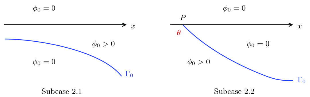
Subcase 2.1. $\displaystyle\phi_{0}>0$ above $\displaystyle\Gamma_{0}$ . Since $\displaystyle\phi_{0}(X)$ is monotone decreasing with respect to $\displaystyle y$ , we can rule out this subcase.

Subcase 2.2. $\displaystyle\phi_{0}>0$ below $\displaystyle\Gamma_{0}$ . The convexity of the free boundary $\displaystyle\Gamma_{0}$ implies that $\displaystyle\Gamma_{0}$ must intersect the $\displaystyle x$ -axis, denote $\displaystyle P$ the intersection point. Moreover, the convexity of $\displaystyle\Gamma_{0}$ and monotonicity of $\displaystyle\phi_{0}$ with respect to $\displaystyle y$ imply that the angle $\displaystyle\theta$ between $\displaystyle\Gamma$ and $\displaystyle x$ -axis at point $\displaystyle P$ lies in $\displaystyle\left[\frac{\pi}{2},\pi\right)$ . Applying the similar arguments in the proof of (2.30) in [17], one has

\phi_{0}(X)\leq C|X-P|^{\frac{2\pi}{\theta+\pi+\varepsilon}}\ \ \ \text{near the intersection point $\displaystyle P$},

(4.44)

for small $\displaystyle\varepsilon\in\left(0,\frac{\pi-\theta}{4}\right)$ . Denote $\displaystyle r=|X-P|$ , using the non-degeneracy Lemma 3.4 and Remark 3.5 in [3], we have

\frac{1}{r}\fint_{\partial B_{r}(P)}\phi_{0}dS\geq c_{*}\lambda.

(4.45)

On the other hand, it follows from (4.44) and (4.45) that

c_{*}\lambda\leq\frac{1}{r}\fint_{\partial B_{r}(P)}\phi_{0}dS\leq C\frac{r^{\frac{2\pi}{\theta+\pi+\varepsilon}}}{r}=Cr^{\frac{\pi-\theta-\varepsilon}{\pi+\theta+\varepsilon}},

which leads a contradiction, provided that $\displaystyle r$ is small enough.

Hence, the proof of the claim (4.37) is done.

With the aid of the claim (4.37), we will show that

\nabla\psi_{\lambda,L}(X)\rightarrow\lambda(0,1)\ \ \text{as}\ \ \ X\rightarrow X_{0},\ \ X\in\Omega_{L}\cap\{\psi_{\lambda,L}<Q\}.

(4.46)

For any sequence of points $\displaystyle X_{n}=(x_{n},y_{n})\in\Omega_{L}\cap\{\psi_{\lambda,L}<Q\}$ with $\displaystyle X_{n}\rightarrow X_{0}$ , let $\displaystyle\tilde{X}_{n}=(\tilde{x}_{n},\tilde{y}_{n})\in\partial D_{L}$ be the nearest point to $\displaystyle X_{n}$ . Denote

r_{n}=|X_{n}-\tilde{X}_{n}|\ \ \ \text{and}\ \ \ d_{n}=\text{dist}(X_{n},\Gamma_{\lambda,L}).

Next, we consider the following two cases.

Case 1. There exists a constant $\displaystyle C_{0}>1$ , such that $\displaystyle r_{n}<C_{0}d_{n}$ . Define a blow-up sequence

\phi_{n}(X)=\frac{Q-\psi_{\lambda,L}(\tilde{X}_{n}+C_{0}d_{n}X)}{C_{0}d_{n}}\ \ \ \text{and}\ \ \ Z_{n}=\frac{X_{n}-\tilde{X}_{n}}{C_{0}d_{n}}.

It is easy to check that $\displaystyle B_{2}(0)$ contains some free boundary points of $\displaystyle\phi_{n}$ and $\displaystyle B_{2c_{0}}(Z_{n})\cap\partial\{\phi_{n}>0\}=\varnothing$ , which does not intersect the free boundary of $\displaystyle\phi_{n}$ , where $\displaystyle c_{0}=\frac{1}{4C_{0}}$ . Moreover,

\Delta\phi_{n}+C_{0}d_{n}f(C_{0}x_{n}\phi_{n})=0\ \text{in $\displaystyle B_{2c_{0}}(Z_{n})\cap\{\phi_{n}>0\}$}.

(4.47)

There exist a blow-up limit $\displaystyle\phi_{0}$ and a point $\displaystyle Z_{0}$ with $\displaystyle|Z_{0}|\leq 1$ , such that

\phi_{n}\rightarrow\phi_{0}\ \ \text{in any compact subsets of $\displaystyle\mathbb{R}^{2}$ and $\displaystyle Z_{n}\rightarrow Z_{0}$.}

Due to the fact that $\displaystyle B_{2c_{0}}(Z_{0})$ does not intersect the free boundary of $\displaystyle\phi_{0}$ and $\displaystyle\partial D_{L}$ is $\displaystyle C^{2}$ -smooth near $\displaystyle X_{0}$ , one has

\text{$\displaystyle\phi_{n}\in C^{1,\alpha}$ in $\displaystyle B_{c_{0}}(Z_{n})\cap\{\phi_{n}>0\}$ uniformly with respect to $\displaystyle n$}.

Then we have

\text{$\displaystyle-\nabla\psi_{\lambda,L}(X_{n})=\nabla\phi_{n}(Z_{n})\rightarrow\nabla\phi_{0}(Z_{0})$, as $\displaystyle n\rightarrow\infty$},

(4.48)

which together with (4.37) gives that (4.46) holds.

Case 2. $\displaystyle\frac{r_{n}}{d_{n}}\rightarrow+\infty$ . Define a blow-up sequence

\phi_{n}(X)=\frac{Q-\psi_{\lambda,L}(\tilde{X}_{n}+r_{n}X)}{r_{n}}\ \ \ \text{and}\ \ \ Y_{n}=\frac{X_{n}-\tilde{X}_{n}}{r_{n}}.

Obviously, $\displaystyle B_{2}(0)$ contains the free boundary points of $\displaystyle\phi_{n}$ for sufficiently large $\displaystyle n$ . Then there exist a blow-up limit $\displaystyle\phi_{0}$ and a point $\displaystyle Y_{0}$ with $\displaystyle|Y_{0}|=1$ , such that

\phi_{n}\rightarrow\phi_{0}=-\lambda\min\{y-y_{1},0\}\ \ \text{in any compact subsets of $\displaystyle\mathbb{R}^{2}$ and $\displaystyle Y_{n}\rightarrow Y_{0}$,}

where $\displaystyle y_{1}\leq 0$ . Since the free boundary $\displaystyle\partial\{\phi_{n}>0\}\rightarrow\partial\{\phi_{0}>0\}$ locally in the Hausdorff distance (see Lemma 3.4) and $\displaystyle\partial\{\phi_{0}>0\}$ is a straight line, we can conclude that the free boundary of $\displaystyle\phi_{n}$ satisfies the flatness condition at $\displaystyle(0,y_{1})$ in the direction $\displaystyle(0,1)$ , for sufficiently large $\displaystyle n$ . By virtue of Theorem 3.15, one has the free boundary of $\displaystyle\phi_{n}$ is $\displaystyle C^{1,\alpha}$ $\displaystyle(0<\alpha<1)$ uniformly in $\displaystyle n$ . The elliptic regularity gives that $\displaystyle\phi_{n}$ is uniformly $\displaystyle C^{1,\alpha}$ in $\displaystyle B_{R}(Y_{n})\cap\{\phi_{n}>0\}$ for some $\displaystyle R>0$ . Thus we have

\text{$\displaystyle-\nabla\psi_{\lambda,L}(X_{n})=\nabla\phi_{n}(Y_{n})\rightarrow\nabla\phi_{0}(Y_{0})=-\lambda(0,1)$, as $\displaystyle n\rightarrow\infty$}.

Since the blow-up limit $\displaystyle\phi_{0}$ is a harmonic function, recalling the fact (4.46), along the similar arguments on the smooth fit condition (see Section 11 in Chapter 3 in [23]), we can show that

k^{\prime}_{\lambda,L}\left(\frac{L}{2}\right)=0.

Hence, we complete the proof of the proposition. ∎

4.6. The continuous fit condition for free boundary

In this subsection, we will check the continuous fit condition of the free boundary $\displaystyle\Gamma_{\lambda,L}$ at $\displaystyle A$ , namely, for any $\displaystyle L>\bar{H}=\max_{x\leq 0}g(x)$ , there exists a $\displaystyle\lambda_{L}\geq\lambda_{0}$ , such that

k_{\lambda_{L},L}(0)=g(0)=a.

(4.49)

To obtain the continuous fit condition (4.49), we first establish the continuous dependence of $\displaystyle\psi_{\lambda,L}$ and $\displaystyle k_{\lambda,L}(0)$ with respect to the parameter $\displaystyle\lambda$ .

Lemma 4.11.

If $\displaystyle\lambda_{n}\rightarrow\lambda$ with $\displaystyle\lambda_{n}\geq\lambda_{0}$ , then

\psi_{\lambda_{n},L}\rightarrow\psi_{\lambda,L}\ \ \text{weakly~~ in}~~H^{1}(\Omega_{L})~~\text{and uniformly in}~\Omega_{L},

and

k_{\lambda_{n},L}(0)\rightarrow k_{\lambda,L}(0)\ \ \text{for}~~k_{\lambda,L}(0)<L.

(4.50)

Proof.

It follows from the similar arguments in the proof of Lemma 3.4, there exists a subsequence $\displaystyle\{\psi_{\lambda_{n},L}\}$ and a $\displaystyle\psi_{0}\in C^{0,1}(\Omega_{L})$ , such that

\psi_{\lambda_{n},L}(X)\rightarrow\psi_{0}(X)\ \text{uniformly in $\displaystyle\Omega_{L}$}.

Furthermore, $\displaystyle\psi_{0}$ is a minimizer to the variational problem $\displaystyle(P_{\lambda,L})$ . The uniqueness of the minimizer to the variational problem $\displaystyle(P_{\lambda,L})$ gives that $\displaystyle\psi_{0}=\psi_{\lambda,L}$ .

Suppose that the assertion (4.50) is not true, then there exists a sequence $\displaystyle\{k_{\lambda_{n},L}(0)\}$ , such that

k_{\lambda_{n},L}(0)\rightarrow k_{\lambda,L}(0)+\delta\ \ \text{as $\displaystyle n\rightarrow+\infty$},\ \ \delta\neq 0.

We consider the following three cases and derive a contradiction.

Case 1. $\displaystyle\delta<0$ . The monotonicity of $\displaystyle\psi_{\lambda,L}(x,y)$ with respect to $\displaystyle y$ gives that $\displaystyle k_{\lambda,L}(0)+\delta\geq a$ .

Next, we claim that

\frac{\partial\psi_{\lambda,L}(0+0,y)}{\partial x}=-\lambda\ \ \ \text{on}\ \ I_{\varepsilon},

(4.51)

where $\displaystyle I_{\varepsilon}=\{(0,y)\mid k_{\lambda,L}(0)-4\varepsilon<y<k_{\lambda,L}(0)-2\varepsilon\}$ with $\displaystyle\varepsilon=-\frac{\delta}{6}$ .

It follows from the statement (4) in Proposition 4.4 that

-\frac{\partial\psi_{\lambda,L}(0+0,y)}{\partial x}=|\nabla\psi_{\lambda,L}|\geq\lambda\ \ \text{on}\ \ I_{\varepsilon}.

(4.52)

To obtain the claim (4.51), it suffices to show that

\frac{\partial\psi_{\lambda,L}(0+0,y)}{\partial x}\geq-\lambda\ \ \ \text{on}\ \ I_{\varepsilon}.

(4.53)

Denote $\displaystyle\phi_{n}=Q-\psi_{\lambda_{n},L}$ , $\displaystyle\phi=Q-\psi_{\lambda,L}$ and

U_{\varepsilon,\tau}=\{(x,y)\mid-\tau<x<\tau,k_{\lambda,L}(0)-5\varepsilon<y<k_{\lambda,L}(0)-\varepsilon\}

for small $\displaystyle\tau>0$ , Proposition 4.4 gives that the free boundary $\displaystyle U_{\varepsilon,\tau}\cap\partial\{\phi_{n}>0\}$ is $\displaystyle C^{3,\alpha}$ , then we have

\displaystyle U_{\varepsilon}\cap\partial\{\phi_{n}>0\}\rightarrow U_{\varepsilon,\tau}\cap\partial\{\phi>0\}

\displaystyle C^{1,\alpha}

for some

\displaystyle\alpha\in(0,1)

For any fixed $\displaystyle X_{1}=(0,y_{1})\in U_{\varepsilon,\tau}\cap\partial\{\phi>0\}$ , then there exists a sequence $\displaystyle X_{n}\in U_{\varepsilon}$ with $\displaystyle\phi_{n}(X_{n})=0$ , such that $\displaystyle X_{n}\rightarrow X_{1}$ as $\displaystyle n\rightarrow+\infty$ . In fact, suppose that there exists a small $\displaystyle r>0$ , such that $\displaystyle\phi_{n}>0$ and $\displaystyle\Delta\phi_{n}+f(\phi_{n})=0$ in $\displaystyle B_{r}(X_{1})$ , which gives that $\displaystyle\Delta\phi+f(\phi)=0$ in $\displaystyle B_{r}(X_{1})$ and $\displaystyle\phi(X_{1})=0$ . The maximum principle implies that $\displaystyle\phi\equiv 0$ in $\displaystyle B_{r}(X_{1})$ , which contradicts to $\displaystyle X_{1}\in U_{\varepsilon,\tau}\cap\partial\{\phi>0\}$ .

Take a small $\displaystyle r>0$ with $\displaystyle E_{n}\subset B_{r}(X_{1})\subset U_{\varepsilon,\tau}$ , such that

E_{n}=B_{r}(X_{1})\cap\{x>\varepsilon_{n}\},\ \phi_{n}>0\ \text{in}\ E_{n}\ \text{and}\ X_{n}\notin E_{n},

(4.54)

where $\displaystyle\varepsilon_{n}\downarrow 0$ as $\displaystyle n\rightarrow+\infty$ . Define a function $\displaystyle h_{s,n}(y)$ as follows

h_{s,n}(y)=\varepsilon_{n}-s\eta\left(\frac{2(y-y_{1})}{r}\right),\ \ s>0,

where

\eta(y)=\left\{\begin{array}[]{ll}e^{-\frac{y^{2}}{1-y^{2}}}&\text{for}\ \ |y|<1\\ 0&\text{for}\ |y|\geq 1.\end{array}\right.

(4.55)

Denote the domain $\displaystyle E_{s,n}=B_{r}(X_{1})\cap\{x>h_{s,n}(y)\}$ . It is easy to check that $\displaystyle E_{0,n}=E_{n}$ . Let $\displaystyle s=s_{n}\leq\varepsilon_{n}$ to be the largest one, such that $\displaystyle\phi_{n}>0$ in $\displaystyle E_{s_{n},n}$ , and $\displaystyle\tilde{X}_{n}=(\tilde{x}_{n},\tilde{y}_{n})\in(B_{r}(X_{1})\cap\partial E_{s_{n},n})\cap\Gamma_{\lambda_{n},L}$ . Furthermore,

\tilde{x}_{n}=h_{s_{n},n}(\tilde{y}_{n})\ \ \text{and}\ \ s_{n}\rightarrow 0\ \ \text{as}\ \ n\rightarrow+\infty.

Let $\displaystyle\varphi_{n}$ be the solution of the following Dirichlet problem

\left\{\begin{array}[]{ll}&\Delta\varphi_{n}+f(\varphi_{n})=0\ \ \text{in}\ E_{s_{n},n},\\ &\varphi_{n}=0\ \text{on}\ \partial E_{s_{n},n}\cap B_{\frac{r}{2}}(X_{1}),\ \varphi_{n}=\zeta\phi_{n}\ \text{on}\ \partial E_{s_{n},n}\cap(B_{r}(X_{1})\setminus B_{\frac{r}{2}}(X_{1})),\\ &\varphi_{n}=\phi_{n}\ \text{on}\ \partial E_{s_{n},n}\cap\partial B_{r}(X_{1}),\end{array}\right.

where $\displaystyle\zeta(X)=\min\left\{\max\left\{\frac{2|X-X_{1}|-r}{r},0\right\},1\right\}$ . It is clear that $\displaystyle\varphi_{n}\leq\phi_{n}$ on $\displaystyle\partial E_{s_{n},n}$ , which gives that

\lambda_{n}=\frac{\partial\phi_{n}(\tilde{X}_{n})}{\partial\nu_{n}}\geq\frac{\partial\varphi_{n}(\tilde{X}_{n})}{\partial\nu_{n}},

(4.56)

where $\displaystyle\nu_{n}$ is the inner normal vector to $\displaystyle\partial E_{s_{n},n}$ at $\displaystyle\tilde{X}_{n}$ .

Taking $\displaystyle\varepsilon_{n}\rightarrow 0$ implies that

h_{s_{n},n}(y)\rightarrow 0\ \ \text{in}\ \ C^{1,\beta}\ \ \text{as}\ \ n\rightarrow+\infty.

Thanks to the standard estimates of the solutions of the semilinear elliptic equation, we conclude that $\displaystyle\varphi_{n}$ in $\displaystyle E_{s_{n},n}\cap B_{\frac{r}{2}}(X_{1})$ converges to $\displaystyle\phi$ in $\displaystyle\{\phi>0\}\cap B_{\frac{r}{2}}(X_{1})$ in $\displaystyle C^{1,\beta}$ -sense. Denote $\displaystyle\tilde{X}_{n}\rightarrow\tilde{X}\in\partial\{\phi>0\}\cap B_{\frac{r}{2}}(X_{1}).$ It follows from (4.56) that

\frac{\partial\varphi_{n}(\tilde{X}_{n})}{\partial\nu}\rightarrow\frac{\partial\phi(\tilde{X})}{\partial\nu}\ \ \text{and}\ \ \frac{\partial\phi(\tilde{X})}{\partial\nu}\leq\lambda.

(4.57)

Taking $\displaystyle r\rightarrow 0$ yields that $\displaystyle\tilde{X}\rightarrow X_{1}$ and

\lambda\geq\frac{\partial\phi(\tilde{X})}{\partial\nu}\rightarrow\frac{\partial\phi(X_{1})}{\partial\nu}=-\frac{\partial\psi_{\lambda,L}(X_{1})}{\partial x},\ \ X_{1}\in U_{\varepsilon,\tau}\cap\partial\{\phi>0\},

which together with (4.53) gives that the claim (4.51) holds.

With the aid of the fact (4.51), we can obtain a contradiction by using the similar arguments in the proof of Lemma 4.8.

Case 2. $\displaystyle\delta>0$ and $\displaystyle k_{\lambda,L}(0)<a$ . Similar to the proof of the claim (4.51) in Case 1, one has

\frac{\partial\psi_{\lambda,L}(0-0,y)}{\partial x}=\lambda\ \ \ \text{on}\ \ I_{\varepsilon},

(4.58)

where $\displaystyle I_{\varepsilon}=\{(0,y)\mid k_{\lambda,L}(0)+\varepsilon<y<k_{\lambda,L}(0)+2\varepsilon\}$ with $\displaystyle\varepsilon=\frac{\min\{\delta,a-k_{\lambda,L}(0)\}}{3}$ , and we can obtain a contradiction.

Case 3. $\displaystyle\delta>0$ and $\displaystyle k_{\lambda,L}(0)\geq a$ . Since $\displaystyle\psi_{\lambda,L}=Q$ on $\displaystyle I_{0,L}$ , it follows from the statement (4) in Proposition 4.4 that

\frac{\partial\psi_{\lambda_{n},L}(0+0,y)}{\partial x}\geq\lambda_{n}\ \ \text{on}\ \ I_{\delta},

for sufficiently large $\displaystyle n$ , where $\displaystyle I_{\delta}=\left\{(0,y)\mid k_{\lambda,L}(0)+\frac{\delta}{4}<y<k_{\lambda,L}(0)+\frac{3\delta}{4}\right\}$ .

Let $\displaystyle E_{n}$ be a domain bounded by $\displaystyle x=0$ , $\displaystyle y=k_{\lambda_{n},L}(x)$ , $\displaystyle y=k_{\lambda,L}(0)+\frac{\delta}{4}$ and $\displaystyle y=k_{\lambda,L}(0)+\frac{3\delta}{4}$ . Moreover,

x_{n}=\max\left\{x\mid k_{\lambda_{n},L}(x)=k_{\lambda,L}(0)+\frac{\delta}{4}\right\}\rightarrow 0\ \ \text{as}\ \ n\rightarrow+\infty.

Thanks to the non-oscillation Lemma 4.7 for $\displaystyle\psi_{\lambda_{n},L}$ in $\displaystyle E_{n}$ , there exists a constant $\displaystyle C$ independent of $\displaystyle n$ , such that

0<\frac{\delta}{2}\leq Cx_{n},

which gives a contradiction for sufficiently large $\displaystyle n$ .

∎

Next, we will study the relation between the initial point $\displaystyle(0,k_{\lambda,L}(0))$ and $\displaystyle\lambda$ for any $\displaystyle L>\bar{H}$ .

Lemma 4.12.

For any $\displaystyle L>\bar{H}$ , the initial point $\displaystyle(0,k_{\lambda,L}(0))$ satisfies that
(1) there exists a constant $\displaystyle C_{0}>0$ (independent of $\displaystyle L$ ), such that $\displaystyle k_{\lambda,L}(0)<a$ for any $\displaystyle\lambda>C_{0}$ .
(2) there exists a $\displaystyle c_{0}\geq\lambda_{0}$ (independent of $\displaystyle L$ ), such that $\displaystyle k_{\lambda,L}(0)\geq a$ for any $\displaystyle\lambda\leq c_{0}$ .

Proof.

(1) Suppose that there exist a free boundary point and a sufficiently large $\displaystyle\lambda$ , such that $\displaystyle k_{\lambda,L}(0)\geq a$ . Then there exist a $\displaystyle X_{0}\in D_{L}$ and a disc $\displaystyle B_{r_{0}}(X_{0})$ with $\displaystyle r_{0}>0$ (independent of $\displaystyle L$ ), such that $\displaystyle\Gamma_{\lambda,L}\cap B_{\frac{r_{0}}{2}}(X_{0})\neq\varnothing$ . It follows from the non-degeneracy Lemma 2.6 and Remark 2.3 that

\frac{Q}{r_{0}}\geq\frac{1}{r_{0}}\fint_{\partial{B_{r_{0}}(X_{0})}}Q-\psi_{\lambda,L}dS\geq c_{\frac{1}{2}}^{*}\lambda,

which leads to a contradiction for sufficiently large $\displaystyle\lambda$ .

Similarly, we can obtain a contradiction if there is no free boundary point, taking $\displaystyle X_{0}=(0,y_{0})$ with $\displaystyle y_{0}\in(a,L)$ and using the non-degeneracy Lemma 2.5 for the boundary point (see Remark 2.3).

(2) Suppose not, then for any $\displaystyle c_{0}\geq\lambda_{0}$ , there exists a $\displaystyle\tilde{\lambda}\in[\lambda_{0},c_{0}]$ , such that $\displaystyle k_{\tilde{\lambda},L}(0)<a$ . In view of Remark 4.4, we have

the asymptotic height

\displaystyle\tilde{h}=h_{\tilde{\lambda}}

in downstream lies in

\displaystyle[a,H]

(4.59)

provided that $\displaystyle c_{0}-\lambda_{0}$ is small. Let $\displaystyle\tilde{\Psi}_{\varepsilon}(y)=\Psi_{\tilde{\lambda}}(y+\varepsilon)$ for $\displaystyle\varepsilon\geq 0$ , choosing $\displaystyle\varepsilon_{0}\geq 0$ to be the smallest one, such that

\psi_{\tilde{\lambda},L}(X)\leq\tilde{\Psi}_{\varepsilon_{0}}(y)\ \text{in $\displaystyle\Omega_{L}\cap\{\tilde{\Psi}_{\varepsilon_{0}}<Q\}$ and $\displaystyle\psi_{\tilde{\lambda},L}(X_{0})=\tilde{\Psi}_{\varepsilon_{0}}(y_{0})$}

for $\displaystyle X_{0}=(x_{0},y_{0})\in\overline{\Omega_{L}\cap\{\tilde{\Psi}_{\varepsilon_{0}}<Q\}}$ . It follows from (4.59) that $\displaystyle\varepsilon_{0}>0$ . We first show that

X_{0}\notin\Omega_{L}\cap\{\tilde{\Psi}_{\varepsilon_{0}}<Q\}.

(4.60)

Suppose not, there exists a point $\displaystyle X_{0}\in\Omega_{L}\cap\{\tilde{\Psi}_{\varepsilon_{0}}<Q\}$ , such that $\displaystyle 0<\tilde{\Psi}_{\varepsilon_{0}}(X_{0})=\psi_{\tilde{\lambda},L}(X_{0})<Q$ . Then there exists a small $\displaystyle r>0$ such that

0<\psi_{\tilde{\lambda},L}<Q\ \text{and}\ \ 0<\tilde{\Psi}_{\varepsilon_{0}}<Q\ \text{in}\ B_{r}(X_{0}).

On the other hand,

\Delta(\psi_{\tilde{\lambda},L}-\tilde{\Psi}_{\varepsilon_{0}})+f_{0}(\psi_{\tilde{\lambda},L})-f_{0}(\tilde{\Psi}_{\varepsilon_{0}})=0\ \ \ \text{in $\displaystyle B_{r}(X_{0})$}.

The strong maximum principle gives that $\displaystyle\psi_{\tilde{\lambda},L}(X_{0})\equiv\tilde{\Psi}_{\varepsilon_{0}}(X_{0})$ in $\displaystyle B_{r}(X_{0})$ , due to $\displaystyle\psi_{\tilde{\lambda},L}(X_{0})=\tilde{\Psi}_{\varepsilon_{0}}(X_{0})$ . Applying the strong maximum principle again, then $\displaystyle\psi_{\tilde{\lambda},L}(X_{0})\equiv\tilde{\Psi}_{\varepsilon_{0}}(X_{0})$ in $\displaystyle\Omega_{L}$ , which leads a contradiction.

The boundary value of $\displaystyle\psi_{\tilde{\lambda},L}$ gives that $\displaystyle X_{0}\notin\partial\Omega_{L}$ . Next, we claim that

X_{0}\neq(0,k_{\tilde{\lambda},L}(0)).

(4.61)

In fact, it follows from Proposition 4.10 that the free boundary $\displaystyle\Gamma_{\tilde{\lambda},L}$ is $\displaystyle C^{1}$ at $\displaystyle X_{0}$ and its tangent is in the direction of the positive $\displaystyle y$ -axis, the definition of $\displaystyle\varepsilon_{0}$ implies the claim (4.61).

Thus, let $\displaystyle X_{0}$ be a free boundary point of $\displaystyle\psi_{\tilde{\lambda},L}$ . Since the free boundary $\displaystyle\Gamma_{\tilde{\lambda},L}$ is $\displaystyle C^{3,\alpha}$ at $\displaystyle X_{0}$ , it follows from Hopf’s lemma that

\tilde{\lambda}=\frac{\partial\tilde{\Psi}_{\varepsilon_{0}}}{\partial\nu}<\frac{\partial\psi_{\tilde{\lambda},L}}{\partial\nu}=\tilde{\lambda}\ \ \text{at}\ \ X_{0},

where $\displaystyle\nu=(0,1)$ is the outer normal vector of $\displaystyle\Gamma_{\tilde{\lambda},L}$ at $\displaystyle X_{0}$ , which leads a contradiction.

∎

With the aid of Lemma 4.12, we can define

\Sigma_{L}=\{\lambda\geq\lambda_{0}\mid k_{\lambda,L}(0)<a\}.

and the set $\displaystyle\Sigma_{L}$ is non-empty for sufficiently large $\displaystyle\lambda$ .

Moreover, set

\lambda_{L}=\inf_{\lambda\in\Sigma_{L}}\lambda.

(4.62)

Furthermore, it follows from Lemma 4.12 that

\lambda_{0}\leq\lambda_{L}\leq C_{0}<\infty,

(4.63)

where $\displaystyle C_{0}$ is a constant independent of $\displaystyle L$ .

By virtue of Lemma 4.11 and Lemma 4.12, we have

Proposition 4.13.

For any $\displaystyle L>\bar{H}=\max_{x\leq 0}g(x)$ , there exists a $\displaystyle\lambda_{L}\geq\lambda_{0}$ as in (4.62), such that the free boundary $\displaystyle\Gamma_{\lambda_{L},L}$ satisfies the continuous fit condition and the smooth fit condition

k_{\lambda_{L},L}(0)=g(0)=a\ \ \ \text{and}\ \ \ k^{\prime}_{\lambda_{L},L}(0)=g^{\prime}(0).

(4.64)

Moreover,

k_{\lambda_{L},L}(x)\leq\bar{H}\ \ \ \text{for any $\displaystyle x\in[0,L]$},

(4.65)

and

\psi_{\lambda_{L},L}(x,y)\leq\min\{\Psi_{\lambda_{L}}(y),Q\}\ \ \text{in $\displaystyle\Omega_{L}$}.

(4.66)

Proof.

Step 1. The definition of $\displaystyle\lambda_{L}$ and the continuous dependence of $\displaystyle k_{\lambda,L}(0)$ with respect to $\displaystyle\lambda$ imply that

k_{\lambda_{L},L}(0)=g(0)=a,

which together with Proposition 4.10 gives that $\displaystyle k^{\prime}_{\lambda_{L},L}(0)=g^{\prime}(0)$ . Thus, the continuous fit condition and the smooth fit condition (4.64) hold.

Step 2. Suppose that the assertion (4.65) is not true, then there exists an $\displaystyle\tilde{x}\in(0,L]$ , such that

k_{\lambda_{L},L}(\tilde{x})>\bar{H}=\max_{x\leq 0}g(x).

(4.67)

On the other hand, the fact $\displaystyle\lambda_{L}\geq\lambda_{0}$ implies that the asymptotic height $\displaystyle h_{\lambda_{L}}\leq H\leq\bar{H}$ . Thus we have

k_{\lambda_{L},L}(\tilde{x})>\bar{H}\geq H\geq h_{\lambda_{L}}.

(4.68)

For $\displaystyle\mu<\lambda_{0}$ and $\displaystyle\lambda_{0}-\mu$ is small, define

\omega_{\mu}(y)=\int_{0}^{y}u_{1,\mu}(t)dt,\ \ u_{1,\mu}=\sqrt{u_{0}^{2}(\chi^{-1}(t;p_{diff}))+2p_{diff}}\ \ \text{with}\ \ p_{diff}=\frac{\mu^{2}-\lambda^{2}_{0}}{2},

where $\displaystyle\chi^{-1}(t;p_{diff})$ is defined as in Subsection 4.3. Denote $\displaystyle\omega_{\mu}^{\varepsilon}(y)=\min\{\omega_{\mu}(y-\varepsilon),Q\}$ for any $\displaystyle\varepsilon\geq 0$ . Let $\displaystyle\varepsilon_{0}\geq 0$ be the smallest one, such that

\omega_{\mu}^{\varepsilon_{0}}(y)\leq\psi_{\lambda_{L},L}(X)\ \ \text{in $\displaystyle\Omega_{L}$, and $\displaystyle\omega_{\mu}^{\varepsilon_{0}}(X_{0})=\psi_{\lambda_{L},L}(X_{0})$}

for some $\displaystyle X_{0}=(x_{0},y_{0})\in\overline{\Omega_{L}\cap\{\psi_{\lambda_{L},L}<Q\}}$ . It follows from (4.68) that $\displaystyle\varepsilon_{0}>0$ . The strong maximum principle implies that $\displaystyle X_{0}\notin\Omega_{L}\cap\{\psi_{\lambda_{L},L}<Q\}$ , and thus $\displaystyle\psi_{\lambda_{L},L}(X_{0})=Q$ . Similar to the proof of Lemma 4.12, we can show that $\displaystyle x_{0}\neq L$ . We next consider the following three cases.

Case 1. $\displaystyle X_{0}\in\Gamma_{\lambda_{L},L}$ . Since the free boundary $\displaystyle\Gamma_{\lambda_{L},L}$ is $\displaystyle C^{3,\alpha}$ at $\displaystyle X_{0}$ , the Hopf’s lemma gives that

\mu=\frac{\partial\omega_{\mu}^{\varepsilon_{0}}}{\partial\nu}>\frac{\partial\psi_{\lambda_{L},L}}{\partial\nu}=\lambda_{L}\ \ \text{at}\ \ X_{0},

where $\displaystyle\nu=(0,1)$ is the outer normal vector of $\displaystyle\Gamma_{\lambda_{L},L}$ at $\displaystyle X_{0}$ , which contradicts to the assumption $\displaystyle\mu<\lambda_{0}\leq\lambda_{L}$ .

Case 2. $\displaystyle X_{0}\in\partial D_{L}$ and $\displaystyle\Gamma_{\lambda_{L},L}\cap B_{r}(X_{0})=\varnothing$ for small $\displaystyle r>0$ . In view of that the boundary $\displaystyle\partial D_{L}$ is $\displaystyle C^{2}$ at $\displaystyle X_{0}$ , it follows from Hopf’s lemma that

\lambda_{L}\geq\lambda_{0}>\mu=\frac{\partial\omega_{\mu}^{\varepsilon_{0}}}{\partial\nu}>\frac{\partial\psi_{\lambda_{L},L}}{\partial\nu}\ \ \text{at}\ \ X_{0}.

(4.69)

On the other hand, the statement (4) in Proposition 4.4 gives that

\frac{\partial\psi_{\lambda_{L},L}}{\partial\nu}\geq\lambda_{L}\ \ \text{at}\ \ X_{0},

which contradicts to (4.69).

Case 3. $\displaystyle X_{0}\in\partial D_{L}$ and $\displaystyle\Gamma_{\lambda_{L},L}\cap B_{r}(X_{0})\neq\varnothing$ for any $\displaystyle r>0$ . In view of Proposition 4.10 and $\displaystyle\omega_{\mu}^{\varepsilon_{0}}(y)\leq\psi_{\lambda_{L},L}(X)$ in $\displaystyle\Omega_{L}$ , one has

\lambda_{0}>\mu=\frac{\partial\omega_{\mu}^{\varepsilon_{0}}}{\partial\nu}\geq\frac{\partial\psi_{\lambda_{L},L}}{\partial\nu}=\lambda_{0}\ \ \text{at}\ \ X_{0},

which leads a contradiction.

Step 3. In this step, we will show the assertion (4.66). Denote $\displaystyle\omega_{\varepsilon}(y)=\min\{\Psi_{\lambda_{L}}(y+\varepsilon),Q\}$ for any $\displaystyle\varepsilon\geq 0$ , and choosing the smallest $\displaystyle\varepsilon_{0}\geq 0$ , such that

\omega_{\varepsilon_{0}}(y)\geq\psi_{\lambda_{L},L}(X)\ \ \text{in $\displaystyle\Omega_{L}\cap\{\psi_{\lambda_{L},L}<Q\}$, and $\displaystyle\omega_{\varepsilon_{0}}(y_{0})=\psi_{\lambda_{L},L}(X_{0})$}

for some $\displaystyle X_{0}=(x_{0},y_{0})\in\overline{\Omega_{L}\cap\{\omega_{\varepsilon_{0}}<Q\}}$ . It suffices to show that

\varepsilon_{0}=0.

If not, suppose that $\displaystyle\varepsilon_{0}>0$ . By virtue of the strong maximum principle and the boundary value of $\displaystyle\psi_{\lambda_{L},L}$ , we can choose $\displaystyle X_{0}$ to be the free boundary point of $\displaystyle\psi_{\lambda_{L},L}$ . Thus, we can derive a contradiction by using Hopf’s lemma.

∎

4.7. The existence of the incompressible jet flow

In previous subsections, we show that there exist a $\displaystyle\lambda_{L}$ and a minimizer $\displaystyle\psi_{\lambda_{L},L}$ for any $\displaystyle L>\bar{H}$ , such that the free boundary $\displaystyle\Gamma_{\lambda_{L},L}$ satisfies the continuous fit condition (4.64). Taking $\displaystyle L\rightarrow+\infty$ , we will obtain the existence of the solution to the jet flow problem in this subsection.

First, we consider the following variational problem.

The variational problem $\displaystyle(P_{\lambda})$ : For any $\displaystyle L_{0}>\bar{H}=\max_{x\leq 0}g(x)$ , find a $\displaystyle\psi_{\lambda}\in K$ such that

J_{\lambda,L_{0}}(\psi_{\lambda})\leq J_{\lambda,L_{0}}(\psi),

for any $\displaystyle\psi\in K$ with $\displaystyle\psi=\psi_{\lambda}$ on $\displaystyle\partial\Omega_{L_{0}}$ , the admissible set

K=\{\psi\in H^{1}_{loc}(\mathbb{R}^{2})\mid\psi=0~~\text{lies below}~T,\psi=Q~~\text{lies above}~N\}.

By using the similar arguments in Lemma 4.11, taking a sequence $\displaystyle\{L_{n}\}$ with $\displaystyle L_{n}\rightarrow\infty$ , such that

\lambda_{L_{n}}\rightarrow\lambda~~\text{and}~~\psi_{\lambda_{L_{n}},L_{n}}\rightarrow\psi_{\lambda}\ \ \text{weakly~~ in}~~H_{loc}^{1}(\mathbb{R}^{2})~\text{and uniformly in any compact subset of $\displaystyle\mathbb{R}^{2}$},

as $\displaystyle n\rightarrow\infty$ , and $\displaystyle\psi_{\lambda}$ is a minimizer to the variational problem $\displaystyle(P_{\lambda})$ . It follows from (4.63) that

\lambda_{0}\leq\lambda<+\infty.

Lemma 4.6 gives that $\displaystyle\psi_{\lambda}(x,y)$ is monotone increasing with respect to $\displaystyle y$ , and the free boundary $\displaystyle\Gamma_{\lambda}$ of $\displaystyle\psi_{\lambda}$ is $\displaystyle x$ -graph. Moreover, $\displaystyle\Gamma_{\lambda}$ can be described by a continuous function $\displaystyle y=k_{\lambda}(x)$ for $\displaystyle x\in(0,+\infty)$ , and

\Gamma_{\lambda}=\Omega\cap\partial\{\psi_{\lambda}<Q\}=\{(x,y)\in\Omega\mid x>0,y=k_{\lambda}(x)\}.

By virtue of Proposition 4.13, one has

k_{\lambda}(0)=g(0)=a,\ \ k^{\prime}_{\lambda}(0)=g^{\prime}(0)\ \ \text{and $\displaystyle k_{\lambda}(x)\leq\bar{H}$ for any $\displaystyle x\in(0,\infty)$},

(4.70)

and

\psi_{\lambda}(x,y)\leq\min\{\Psi_{\lambda}(y),Q\}\ \ \text{in $\displaystyle\Omega$}.

(4.71)

Theorem 3.15 and Proposition 2.2 give that the free boundary $\displaystyle\Gamma_{\lambda}$ is $\displaystyle C^{3,\alpha}$ and $\displaystyle|\nabla\psi_{\lambda}|=\frac{\partial\psi_{\lambda}}{\partial\nu}=\lambda$ on $\displaystyle\Gamma_{\lambda}$ , where $\displaystyle\nu$ is the outer normal vector.

Next, we will obtain the positivity of horizontal velocity.

Lemma 4.14.

$\displaystyle u=\frac{\partial\psi_{\lambda}}{\partial y}>0$ in $\displaystyle\overline{\Omega\cap\{\psi_{\lambda}<Q\}}$ .

Proof.

Denote $\displaystyle u=\frac{\partial\psi_{\lambda}}{\partial y}$ , one has

\Delta u+b(X)u=0\ \ \text{in}~\Omega\cap\{\psi_{\lambda}<Q\},

where $\displaystyle b(X)=f_{0}^{\prime}(\psi(X))\leq 0$ . The monotonicity of $\displaystyle\psi_{\lambda}(x,y)$ with respect to $\displaystyle y$ implies that $\displaystyle u\geq 0$ in $\displaystyle\Omega\cap\{\psi_{\lambda}<Q\}$ , the strong maximum principle gives that

\text{$\displaystyle u>0$ in $\displaystyle\Omega\cap\{\psi_{\lambda}<Q\}$}.

Since $\displaystyle\psi_{\lambda}<Q$ in $\displaystyle\Omega\cap\{x<0\}$ and $\displaystyle\psi_{\lambda}=Q$ on $\displaystyle N$ , it follows from $\displaystyle f^{\prime}_{0}(Q)\leq 0$ and Hopf’s lemma that

u=\frac{1}{\sqrt{1+(g^{\prime}(x))^{2}}}\frac{\partial\psi_{\lambda}}{\partial\nu}>0\ \ \text{on $\displaystyle N\setminus A$}.

Similarly, we have

u>0\ \ \text{on $\displaystyle T$.}

Next, we will show that $\displaystyle u>0$ on $\displaystyle\Gamma_{\lambda}$ . Suppose that there exists $\displaystyle x_{0}>0$ , such that $\displaystyle u=\partial_{y}\psi_{\lambda}=0$ on $\displaystyle(x_{0},k_{\lambda}(x_{0}))$ . Since the free boundary $\displaystyle\Gamma_{\lambda}$ is $\displaystyle C^{3,\alpha}$ -smooth at $\displaystyle(x_{0},k_{\lambda}(x_{0}))$ , the normal outer vector is $\displaystyle(1,0)$ at $\displaystyle(x_{0},k_{\lambda}(x_{0}))$ and $\displaystyle|\partial_{x}\psi_{\lambda}|=\lambda$ on $\displaystyle\Gamma_{\lambda}$ . Thanks to Hopf’s lemma, we have

\left|u_{x}\right|=\left|\frac{\partial u}{\partial\nu}\right|>0\ \ \text{at}\ \ (x_{0},k_{\lambda}(x_{0})).

(4.72)

Since $\displaystyle u^{2}+v^{2}=\lambda^{2}$ on $\displaystyle\Gamma_{\lambda}$ , we have

\begin{array}[]{rl}0=\frac{\partial(u^{2}+v^{2})}{\partial s}=2uu_{y}+2vv_{y}=2vv_{y}=-2\lambda u_{x}\ \ \text{at $\displaystyle(x_{0},k_{\lambda}(x_{0}))$,}\end{array}

which contradicts to (4.72).

By virtue of the boundedness of $\displaystyle g^{\prime}(0)$ , we have $\displaystyle u>0$ at $\displaystyle A$ .

The positivity of horizontal velocity $\displaystyle u$ implies that the function $\displaystyle y=k_{\lambda}(x)$ is $\displaystyle C^{1}$ for any $\displaystyle x\geq 0$ . ∎

Next, we will obtain the asymptotic height of the free boundary $\displaystyle\Gamma_{\lambda}$ .

Lemma 4.15.

$\displaystyle\lim_{x\rightarrow\infty}k_{\lambda}(x)=h_{\lambda}$ , where $\displaystyle h_{\lambda}$ is the asymptotic height of the free boundary $\displaystyle\Gamma_{\lambda}$ and $\displaystyle h_{\lambda}\leq a$ .

Proof.

Suppose that the limit $\displaystyle\lim_{x\rightarrow\infty}k_{\lambda}(x)$ does not exist. It follows from the non-degeneracy 2.6 and (4.70) that

0<c_{0}\leq k_{\lambda}(x)\leq\bar{H}\ \ \ \text{for any $\displaystyle x\in[0,\infty)$},

which implies that there exist two sequence $\displaystyle\{x_{n}\}$ and $\displaystyle\{\tilde{x}_{n}\}$ , such that

\lim_{x_{n}\rightarrow\infty}k_{\lambda}(x_{n})=\limsup_{x\rightarrow\infty}k_{\lambda}(x)=h_{\lambda,1}\ \ \text{and}\ \ \lim_{\tilde{x}_{n}\rightarrow\infty}k_{\lambda}(\tilde{x}_{n})=\liminf_{x\rightarrow\infty}k_{\lambda}(x)=h_{\lambda,2}

(4.73)

with $\displaystyle h_{\lambda,1}>h_{\lambda,2}$ .

By virtue of Remark 4.4, there exist $\displaystyle\lambda_{1},\lambda_{2}$ with $\displaystyle\lambda_{0}\leq\lambda_{1}<\lambda_{2}<\infty$ , such that

0<c_{0}\leq h_{\lambda,2}=h_{\lambda_{2}}<h_{\lambda_{1}}=h_{\lambda,1}\leq\bar{H}.

(4.74)

Set $\displaystyle\psi_{n}(t,s)=\psi_{\lambda}(x_{n}+t,s)$ and the free boundary $\displaystyle\Gamma_{n}:s=k_{\lambda}(x_{n}+t)$ . Define a curve

\gamma_{\delta}:s=\bar{H}-\delta\eta\left(\frac{t}{\sqrt{x_{n}}}\right)

where the function $\displaystyle\eta(x)$ is defined as in (4.55). Let $\displaystyle\delta_{n}$ be the largest one, such that the curve $\displaystyle\gamma_{\delta_{n}}$ touches the free boundary $\displaystyle\Gamma_{n}$ at some points $\displaystyle(t_{n},s_{n})$ , and thus

\displaystyle s_{n}=k_{\lambda}(x_{n}+t_{n})

and

\displaystyle\delta_{n}\leq\bar{H}-k_{\lambda}(x_{n})

(4.75)

Let $\displaystyle\omega_{n}$ be the solution to the Dirichlet problem

\left\{\begin{array}[]{ll}&\Delta\omega+f_{0}(\omega)=0\ \text{in}\ \ \ E_{n},\\ &\omega=Q\ \text{on}\ \gamma_{\delta_{n}},\ \ \omega=\psi_{n}\ \ \text{on}\ \ \partial E_{n}\setminus\gamma_{\delta_{n}},\end{array}\right.

(4.76)

where domain $\displaystyle E_{n}$ is bounded by $\displaystyle t=-\frac{x_{n}}{2}$ , $\displaystyle t=\frac{x_{n}}{2}$ , $\displaystyle s=0$ and $\displaystyle\gamma_{\delta_{n}}$ .

Since $\displaystyle\Delta\psi_{n}+f_{0}(\psi_{n})\leq 0$ in $\displaystyle E_{n}$ and $\displaystyle\psi_{n}(t_{n},s_{n})=\omega_{n}(t_{n},s_{n})=Q$ , the maximum principle implies that $\displaystyle\psi_{n}\geq\omega_{n}$ in $\displaystyle E_{n}$ and

\lambda=\frac{\partial\psi_{n}}{\partial\nu_{n}}\leq\frac{\partial\omega_{n}}{\partial\nu_{n}}\ \ \text{at}\ \ (t_{n},s_{n}),

(4.77)

where $\displaystyle\nu_{n}$ is the outer normal vector of $\displaystyle\Gamma_{n}$ .

By virtue of (4.75), we can choose a subsequence $\displaystyle\{x_{n}\}$ , such that

\frac{t_{n}}{\sqrt{x_{n}}}\rightarrow t_{0}\in[-1,1]\ \ \text{and}\ \ \bar{H}-\delta_{n}\eta\left(\frac{t}{\sqrt{x_{n}}}\right)\rightarrow\bar{h}_{\lambda_{1}}.

(4.78)

After a translation in the $\displaystyle t$ direction, such that the free boundary point $\displaystyle(t_{n},s_{n})$ lies on the $\displaystyle s$ -axis, then we have

E_{n}\rightarrow E_{0}=\{(t,s)\mid-\infty<t<\infty,0<s<h_{\lambda_{1}}\}\ \ \text{and}\ \ (t_{n},s_{n})\rightarrow(0,h_{\lambda_{1}}),

(4.79)

and $\displaystyle\omega_{n}\rightarrow\omega_{0}$ uniformly in any compact subset of $\displaystyle E_{0}$ . Moreover, $\displaystyle\omega_{0}$ satisfies that $\displaystyle 0\leq\omega_{0}(t,s)\leq Q$ and

\left\{\begin{array}[]{ll}&\Delta\omega_{0}+f_{0}(\omega_{0})=0\ \text{in}\ \ \ E_{0},\\ &\omega_{0}(t,0)=0,\ \ \omega_{0}(t,h_{\lambda_{1}})=Q.\end{array}\right.

(4.80)

By using the similar arguments in [35], we can show that the Dirichlet problem (4.80) has a unique solution

\omega_{0}(s)=\int_{0}^{s}u_{1}(x)dx,

where $\displaystyle u_{1}(t)=\sqrt{u_{0}^{2}(\chi^{-1}(t;p_{diff}))+2p_{diff}}$ with $\displaystyle p_{diff}=\frac{\lambda_{1}^{2}-\lambda^{2}_{0}}{2}$ , and $\displaystyle\chi^{-1}(t;p_{diff})$ is defined as in Subsection 4.3.

It follows from (4.77) and (4.79) that

\lambda\leq\lim_{n\rightarrow\infty}\frac{\partial\omega_{n}(t_{n},s_{n})}{\partial\nu_{n}}=\frac{\omega_{0}(0,h_{\lambda_{1}})}{\partial s}=\lambda_{1}.

(4.81)

Next, we will show that

\lambda\geq\lambda_{2}.

(4.82)

Define $\displaystyle\tilde{\psi}_{n}(t,s)=\psi_{\lambda}(\tilde{x}_{n}+t,s)$ , $\displaystyle\tilde{\Gamma}_{n}:s=k_{\lambda}(\tilde{x}_{n}+t)$ as the free boundary of $\displaystyle\tilde{\psi}_{n}$ and a curve

\tilde{\gamma}_{\delta}:s=\frac{h_{2}}{2}+\delta\eta\left(\frac{t}{\sqrt{\tilde{x}_{n}}}\right).

Let $\displaystyle\delta_{n}$ be the largest one, such that the curve $\displaystyle\tilde{\gamma}_{\delta_{n}}$ touches the free boundary $\displaystyle\tilde{\Gamma}_{n}$ at a point $\displaystyle(t_{n},s_{n})$ , and thus

\displaystyle s_{n}=k_{\lambda}(\tilde{x}_{n}+t_{n})

and

\displaystyle\delta_{n}\leq k_{\lambda}(\tilde{x}_{n})-\frac{h_{\lambda,2}}{2}

Denote a domain $\displaystyle\tilde{E}_{n}$ , which is bounded by $\displaystyle t=-\frac{\tilde{x}_{n}}{2}$ , $\displaystyle t=\frac{\tilde{x}_{n}}{2}$ , $\displaystyle s=0$ and $\displaystyle\tilde{\gamma}_{\delta_{n}}$ . Let $\displaystyle\tilde{\omega}_{n}$ be the solutions to the Dirichlet problem (4.76), replacing $\displaystyle E_{n}$ and $\displaystyle\gamma_{\delta_{n}}$ by $\displaystyle\tilde{E}_{n}$ and $\displaystyle\tilde{\gamma}_{\delta_{n}}$ . Obviously, $\displaystyle\Delta\psi_{n}+f_{0}(\psi_{n})=0$ in $\displaystyle\tilde{E}_{n}$ , it follows from the maximum principle that $\displaystyle\tilde{\omega}_{n}\geq\tilde{\psi}_{n}$ in $\displaystyle\tilde{E}_{n}$ and

\lambda=\frac{\partial\tilde{\psi}_{n}}{\partial\nu_{n}}\geq\frac{\partial\tilde{\omega}_{n}}{\partial\nu_{n}}\ \ \text{at}\ \ (t_{n},s_{n}),

(4.83)

where $\displaystyle\nu_{n}$ is the outer normal vector of $\displaystyle\Gamma_{n}$ . By using the previous arguments, we can show that there exists a subsequence $\displaystyle\{\tilde{x}_{n}\}$ , such that

\tilde{E}_{n}\rightarrow\tilde{E}_{0}=\{(t,s)\mid-\infty<t<\infty,0<s<h_{\lambda_{2}}\}\ \ \text{and}\ \ (t_{n},s_{n})\rightarrow(0,h_{\lambda_{2}}),

and $\displaystyle\tilde{\omega}_{n}\rightarrow\tilde{\omega}_{0}$ uniformly in any compact subset of $\displaystyle E_{0}$ and

\lim_{n\rightarrow\infty}\frac{\partial\tilde{\omega}_{n}(t_{n},s_{n})}{\partial\nu_{n}}=\frac{\tilde{\omega}_{0}(0,h_{\lambda_{2}})}{\partial s}=\lambda_{2},

which together with (4.83) give that (4.82) holds.

Hence, it follows from (4.81) and (4.82) that

\lambda_{2}\leq\lambda\leq\lambda_{1},

which contradicts to the fact $\displaystyle\lambda_{1}<\lambda_{2}$ .

Thus, there exists an asymptotic height $\displaystyle\tilde{h}$ of the free boundary $\displaystyle\Gamma_{\lambda}$ , such that

k_{\lambda}(x)\rightarrow\tilde{h}.

Next, we claim that

\text{$\displaystyle\tilde{h}=h_{\lambda}$}.

If not, without loss of generality, we assume that $\displaystyle\tilde{h}>h_{\lambda}$ , and there exists a $\displaystyle\tilde{\lambda}<\lambda$ , such that $\displaystyle\tilde{h}=h_{\tilde{\lambda}}$ . Similar to the proof of (4.81) and (4.82), we can show that

\lambda\leq\tilde{\lambda},

which contradicts to the assumption $\displaystyle\tilde{\lambda}<\lambda$ .

Finally, it follows from (4.71) that

h_{\lambda}\leq a.

∎

Finally, the asymptotic behavior of the jet flow will be obtained in the following.

Proposition 4.16.

The rotational jet flow satisfies the following asymptotic behavior in the far fields,

(u,v,p)\rightarrow(u_{0}(y),0,p_{in}),\ \nabla u\rightarrow(0,u_{0}^{\prime}(y)),~~\nabla v\rightarrow 0,~~\nabla p\rightarrow 0,

uniformly in any compact subset of $\displaystyle(0,H)$ , as $\displaystyle x\rightarrow-\infty$ , and

(u,v,p)\rightarrow(u_{1}(y),0,p_{atm}),\ \nabla u\rightarrow(0,u_{1}^{\prime}(y)),~~\nabla v\rightarrow 0,~~\nabla p\rightarrow 0,

uniformly in any compact subset of $\displaystyle(0,h_{\lambda})$ , as $\displaystyle x\rightarrow+\infty,$ where $\displaystyle u_{1}(y)$ and $\displaystyle h_{\lambda}$ are uniquely determined by $\displaystyle u_{0}(y)$ , $\displaystyle p_{in}$ and $\displaystyle p_{atm}$ as in Remark 4.4.

Proof.

For any sequence $\displaystyle\{\psi_{\lambda}(x-n,y)\}$ , by using the uniform elliptic estimate, there exists a subsequence $\displaystyle\{\psi_{\lambda}(x-n,y)\}$ , such that

\psi_{\lambda}(x-n,y)\rightarrow\psi_{0}(x,y)\ \ \text{in $\displaystyle C^{2,\alpha}(S)$},

where $\displaystyle S$ is any compact subsect of $\displaystyle(0,H)$ , $\displaystyle 0\leq\psi_{0}\leq Q$ and

\left\{\begin{array}[]{ll}&\Delta\psi_{0}+f_{0}(\psi_{0})=0\ \text{in}~~\{-\infty<x<+\infty\}\times\{0<y<H\},\\ &\psi_{0}(x,H)=Q\ \text{and}\ \psi_{0}(x,0)=0\ \ \text{for $\displaystyle-\infty<x<+\infty$}.\end{array}\right.

(4.84)

Then boundary value problem (4.84) possesses a unique solution

\psi_{0}(y)=\int_{0}^{y}u_{0}(s)ds,

which implies that

(u,v)(x,y)\rightarrow\left(u_{0}(y),0\right),\ \nabla u(x,y)\rightarrow\left(0,u_{0}^{\prime}(y))\right)\ \text{and}\ \nabla v(x,y)\rightarrow(0,0)

uniformly in any compact subset of $\displaystyle(0,H)$ , as $\displaystyle x\rightarrow-\infty$ . The Bernoulli’s law gives that

p(x,y)\rightarrow p_{in}=\frac{\lambda^{2}}{2}-\frac{u_{0}^{2}(H)}{2}+p_{atm}\ \text{and}\ \nabla p(x,y)\rightarrow 0,

uniformly in any compact subset of $\displaystyle(0,H)$ , as $\displaystyle x\rightarrow-\infty$ .

For any sequence $\displaystyle\{\psi_{n}\}$ with $\displaystyle\psi_{n}(x,y)=\psi_{\lambda}(x+n,y)$ and $\displaystyle R>0$ , by virtue of Lemma 4.15, one has

\lim_{n\rightarrow\infty}k_{\lambda}(x+n)=h_{\lambda}.

(4.85)

For any large $\displaystyle R$ and small $\displaystyle\varepsilon>0$ , it follows from (4.85) that there exists a $\displaystyle N=N(R,\varepsilon)$ , such that the free boundary of $\displaystyle\psi_{n}(X)$ lies in a $\displaystyle\varepsilon$ -neighborhood of the line $\displaystyle\{y=h_{\lambda}\}$ in $\displaystyle B_{R}(0)$ , and thus the free boundary of $\displaystyle\psi_{n}$ satisfies the flatness condition in $\displaystyle B_{R}(0)$ , provided that $\displaystyle n$ is sufficiently large. It follows from Theorem 3.15 that the free boundary of $\displaystyle\psi_{n}$ convergence to the line $\displaystyle\{y=h_{\lambda}\}$ in $\displaystyle C^{1}$ norm, namely,

k^{\prime}_{\lambda}(x+n)\rightarrow 0\ \ \text{as}\ n\rightarrow\infty,\ \ \text{for any $\displaystyle|x|<R$}.

Applying Theorem 3.15 again, one has

\left|k^{(j)}_{\lambda}(x)\right|\leq C\ \ \text{for sufficiently large $\displaystyle x>0$},\ \ j=2,3.

By using the uniform elliptic estimate, there exists a subsequence $\displaystyle\{\psi_{n}\}$ , such that

\psi_{n}(x,y)\rightarrow\psi_{1}(x,y),

and

\left\{\begin{array}[]{ll}&\Delta\psi_{1}+f_{0}(\psi_{1})=0\ \text{in}~~E,\\ &\psi_{1}(x,h_{\lambda})=Q\ \ \text{and}\ \ \psi_{1}(x,0)=0\ \ \text{for $\displaystyle-\infty<x<+\infty$},\end{array}\right.

(4.86)

where $\displaystyle E=\{-\infty<x<+\infty\}\times\{0<y<h_{\lambda}\}$ .

Recalling Remark 4.4,

\psi_{1}(y)=\int_{0}^{y}u_{1}(y)ds\ \ \ \text{in}\ \ E,

(4.87)

solves uniquely Dirichlet problem (4.86) in $\displaystyle E$ , where $\displaystyle u_{1}(t)=\sqrt{u_{0}^{2}(\chi^{-1}(y;p_{diff}))+2p_{diff}}$ with $\displaystyle p_{diff}=\frac{\lambda^{2}-u_{0}^{2}(H)}{2}$ .

In view of (4.87), we conclude that

(u,v,p)(x,y)\rightarrow\left(u_{1}(y),0,p_{atm}\right),\ \nabla u(x,y)\rightarrow\left(0,u_{1}^{\prime}(y)\right),\ \nabla v(x,y)\rightarrow(0,0)

and $\displaystyle\nabla p(x,y)\rightarrow(0,0)$ uniformly in any compact subset of $\displaystyle(0,h_{\lambda})$ , as $\displaystyle x\rightarrow+\infty$ .

∎

4.8. The uniqueness of the incompressible jet flow

In this subsection, we will obtain the uniqueness of $\displaystyle\lambda$ and the solution to the jet flow problem.

Proposition 4.17.

$\displaystyle\lambda$ and the solution $\displaystyle(u,v,p,\Gamma)$ to the jet flow problem are unique.

Proof.

Suppose that $\displaystyle(\psi_{\lambda_{1}},\lambda_{1},\Gamma_{\lambda_{1}})$ and $\displaystyle(\tilde{\psi}_{\lambda_{2}},\lambda_{2},\tilde{\Gamma}_{\lambda_{2}})$ are two solutions to the jet flow problem, which satisfy the conditions in Definition 4.1.

Step 1. In this step, we will show that $\displaystyle\lambda_{1}=\lambda_{2}$ . Suppose not, without loss of generality, we assume that $\displaystyle\lambda_{1}<\lambda_{2}$ . In view of the asymptotic behaviors of $\displaystyle\psi_{\lambda_{1}}$ and $\displaystyle\tilde{\psi}_{\lambda_{2}}$ in Proposition 4.16, one has

k_{\lambda_{1}}(x)>\tilde{k}_{\lambda_{2}}(x)\ \ \text{for sufficiently large $\displaystyle x>0$.}

(4.88)

Consider a function $\displaystyle\psi_{\lambda_{1}}^{\varepsilon}(x,y)=\psi_{\lambda_{1}}(x,y-\varepsilon)$ for $\displaystyle\varepsilon\geq 0$ and $\displaystyle\Gamma_{\lambda_{1}}^{\varepsilon}$ is the free boundary of $\displaystyle\psi_{\lambda_{1}}^{\varepsilon}$ , choosing the smallest $\displaystyle\varepsilon_{0}\geq 0$ such that

\psi_{\lambda_{1}}^{\varepsilon_{0}}(X)\leq\tilde{\psi}_{\lambda_{2}}(X)\ \text{in $\displaystyle\Omega$, and}\ \psi_{\lambda_{1}}^{\varepsilon_{0}}(X_{0})=\tilde{\psi}_{\lambda_{2}}(X_{0})\ \text{for some $\displaystyle X_{0}\in\overline{\Omega\cap\{\tilde{\psi}_{\lambda_{2}}<Q\}}$}.

(4.89)

Similar to the proof of (4.60), the strong maximum principle implies that $\displaystyle X_{0}\notin\Omega\cap\{\tilde{\psi}_{\lambda_{2}}<Q\}$ . We next consider the following two cases.

Case 1. $\displaystyle\varepsilon_{0}=0$ , we can choose $\displaystyle X_{0}=A$ . Then one has

\frac{\partial\psi_{\lambda_{1}}}{\partial\nu}=|\nabla\psi_{\lambda_{1}}|=\lambda_{1}\ \ \text{and}\ \ \frac{\partial\tilde{\psi}_{\lambda_{2}}}{\partial\nu}=|\nabla\tilde{\psi}_{\lambda_{2}}|=\lambda_{2}\ \ \ \text{at $\displaystyle A$,}

where $\displaystyle\nu$ is the outer normal vector. Since $\displaystyle\psi_{\lambda_{1}}\leq\tilde{\psi}_{\lambda_{2}}$ in $\displaystyle\Omega$ , which yields that

\lambda_{1}=\frac{\partial\psi_{\lambda_{1}}}{\partial\nu}\geq\frac{\partial\tilde{\psi}_{\lambda_{2}}}{\partial\nu}=\lambda_{2}\ \ \ \text{at $\displaystyle A$,}

which leads a contradiction to the assumption $\displaystyle\lambda_{1}<\lambda_{2}$ .

Case 2. $\displaystyle\varepsilon_{0}>0$ , it follows from (4.88) that $\displaystyle|X_{0}|<+\infty$ . Then we can take $\displaystyle X_{0}$ be the free boundary point of $\displaystyle\psi^{\varepsilon_{0}}_{\lambda_{1}}$ and $\displaystyle\tilde{\psi}_{\lambda_{2}}$ , and the strong maximum principle gives that

\psi_{\lambda_{1}}^{\varepsilon_{0}}(X)<\tilde{\psi}_{\lambda_{2}}(X)\ \ \text{in $\displaystyle\Omega\cap\{\tilde{\psi}_{\tilde{\lambda}_{2}}<Q\}$}.

Since the free boundaries $\displaystyle\Gamma^{\varepsilon_{0}}_{\lambda_{1}}$ and $\displaystyle\tilde{\Gamma}_{\lambda_{2}}$ are $\displaystyle C^{3,\alpha}$ at $\displaystyle X_{0}$ , it follows from Hopf’s lemma that

\lambda_{1}=\frac{\partial\psi_{\lambda_{1}}^{\varepsilon_{0}}}{\partial\nu}>\frac{\partial\tilde{\psi}_{\lambda_{2}}}{\partial\nu}=\lambda_{2}\ \ \ \text{at $\displaystyle X_{0}$,}

where $\displaystyle\nu$ is the outer normal vector to $\displaystyle\Gamma_{\lambda_{1}}^{\varepsilon_{0}}\cap\tilde{\Gamma}_{\lambda_{2}}$ at $\displaystyle X_{0}$ . This leads a contradiction to the assumption $\displaystyle\lambda_{1}<\lambda_{2}$ .

Hence, we obtain the uniqueness of $\displaystyle\lambda$ , and denote $\displaystyle\lambda=\lambda_{1}=\lambda_{2}$ .

Step 2. In this step, we will show that $\displaystyle\psi_{\lambda}=\tilde{\psi}_{\lambda}$ . By virtue of the asymptotic behaviors of $\displaystyle\psi_{\lambda_{1}}$ and $\displaystyle\tilde{\psi}_{\lambda_{2}}$ in Proposition 4.16, we have

\lim_{x\rightarrow+\infty}k_{\lambda}(x)=\lim_{x\rightarrow+\infty}\tilde{k}_{\lambda}(x)=h_{\lambda}.

Without loss of generality, we assume that there exists some $\displaystyle x_{0}\in(0,+\infty)$ , such that

k_{\lambda}(x_{0})<\tilde{k}_{\lambda}(x_{0}).

(4.90)

Denote $\displaystyle\psi_{\lambda}^{\varepsilon}(x,y)=\psi_{\lambda}(x,y-\varepsilon)$ for $\displaystyle\varepsilon\geq 0$ , and let $\displaystyle\varepsilon_{0}\geq 0$ to be the smallest one, such that

\psi_{\lambda}^{\varepsilon_{0}}(X)\leq\tilde{\psi}_{\lambda}(X)\ \text{in $\displaystyle\Omega$, and}\ \psi_{\lambda}^{\varepsilon_{0}}(X_{0})=\tilde{\psi}_{\lambda}(X_{0})\ \text{for some $\displaystyle X_{0}\in\overline{\Omega\cap\{\tilde{\psi}_{\lambda}<Q\}}$}.

(4.91)

It follows from assumption (4.90) that $\displaystyle\varepsilon_{0}>0$ and $\displaystyle|X_{0}|<+\infty$ .

Similar to the proof of Case 1 in Step 1, we can take $\displaystyle X_{0}$ be the free boundary point of $\displaystyle\psi_{\lambda}^{\varepsilon_{0}}$ and $\displaystyle\tilde{\psi}_{\lambda}$ , applying Hopf’s lemma yields that

\lambda=\frac{\partial\psi_{\lambda}^{\varepsilon_{0}}}{\partial\nu}>\frac{\partial\tilde{\psi}_{\lambda}}{\partial\nu}=\lambda\ \ \ \text{at $\displaystyle X_{0}$,}

where $\displaystyle\nu$ is the outer normal vector to $\displaystyle\Gamma_{\lambda}^{\varepsilon_{0}}\cap\tilde{\Gamma}_{\lambda}$ at $\displaystyle X_{0}$ . This leads a contradiction. ∎

References

[1] S. Agmon, A. Douglis, L. Nirenberg, Estimates near the boundary for solutions of elliptic partial differential equations satisfying general boundary conditions. I, Comm. Pure Appl. Math., 12, 623-727, (1959).
[2] H. W. Alt, L. A. Caffarelli, Existence and regularity for a minimum problem with free boundary, J. Reine Angew. Math., 325, 105-144, (1981).
[3] H. W. Alt, L. A. Caffarelli, A. Friedman, Asymmetric jet flows, Comm. Pure Appl. Math., 35, 29-68, (1982).
[4] H. W. Alt, L. A. Caffarelli, A. Friedman, Jet flows with gravity, J. Reine Angew. Math., 35, 58-103, (1982).
[5] H. W. Alt, L. A. Caffarelli, A. Friedman, Axially symmetric jet flows, Arch. Ration. Mech. Anal., 81, 97-149, (1983).
[6] H. W. Alt, L. A. Caffarelli, A. Friedman, A free boundary problem for quasilinear elliptic equations, Ann. Scuola Norm. Sup. Pisa Cl. Sci., 11, 1-44, (1984).
[7] H. W. Alt, L. A. Caffarelli, A. Friedman, Compressible flows of jets and cavities, J. Differential Equations, 56, 82-141, (1985).
[8] H. W. Alt, D. Phillips, A free boundary problem for semilinear elliptic equations, J. Reine Angew. Math., 368, 63-107, (1986).
[9] L. A. Caffarelli, A Harnack inequality approach to the regularity of free boundaries, I. Lipschitz free boundaries are $\displaystyle C^{1,\alpha}$ , Rev. Mat. Iberoamericana, 3, 139-162, (1987).
[10] L. A. Caffarelli, A Harnack inequality approach to the regularity of free boundaries. II. Flat free boundaries are Lipschitz, Comm. Pure Appl. Math., 42, 55-78, (1989).
[11] M. C. Cerutti, F. Ferrari, S. Salsa, Two-phase problems for linear elliptic operators with variable coefficients: Lipschitz free boundaries are $\displaystyle C^{1,\gamma}$ , Arch. Ration. Mech. Anal., 171, 329-348, (2004).
[12] J. F. Cheng, L. L. Du, Hydrodynamic jet incident on an uneven wall, Math. Models Methods Appl. Sci., 28, 771-827, (2018).
[13] J. F. Cheng, L. L. Du, Y, F, Wang, Two-dimensional impinging jets in hydrodynamic rotational flows, Ann. Inst. H. Poincaré Anal. Non Linéaire, 34, 1355-1386, (2017).
[14] J. F. Cheng, L. L. Du, Y, F, Wang, On incompressible oblique impinging jet flows, J. Differential Equations, 265, 4687-4748, (2018).
[15] J. F. Cheng, L. L. Du, W, Xiang, Incompressible jet flows in a de Laval nozzle with smooth detachment, Arch. Ration. Mech. Anal., 232, 1031-1072, (2019).
[16] J. F. Cheng, L. L. Du, Q. Zhang, Two-dimensional cavity flow in an infinitely long channel with non-zero vorticity, J. Differential Equations, 263, 4126-4155, (2017).
[17] L. L. Du, C. J. Xie, On subsonic Euler flows with stagnation points in two dimensional nozzles, Indiana Univ. Math. J., 63, 1499-1523, (2014).
[18] L. L. Du, C. J. Xie, Z. P. Xin, Steady subsonic ideal flows through an infinitely long nozzle with large vorticity, Comm. Math. Phys., 328, 327-354, (2014).
[19] L. C. Evans, Measure theory and fine properties of functions, Studies in Advanced Mathematics, American Mathematical Society, Providence, 1992.
[20] H. Federer, Geometric measure theory, Berlin-Heidelberg, New York, 1969.
[21] F. Ferrari, S. Salsa, Regularity of the free boundary in two-phase problems for linear elliptic operators, Adv. Math., 214, 288-322, (2007).
[22] F. Ferrari, S. Salsa, Subsolutions of elliptic operators in divergence form and application to two-phase free boundary problems, Bound. Value Probl., Article 57049, 21 pp., (2007).
[23] A. Friedman, Variational principles and free-boundary problems, Pure and Applied Mathematics, John Wiley Sons, Inc., New York, 1982.
[24] A. Friedman, Axially symmetric cavities in rotational flows, Comm. Partial Differential Equations, 8, 949-997, (1983).
[25] D. Gilbarg, The Phragm $\displaystyle\grave{\text{e}}$ n-Lindelöf theorem for elliptic partical differential equations, J. Rational Mech. Anal., 1, 411-417, (1952).
[26] D. Gilbarg, N. S. Trudinger, Elliptic Partial Differential Equations of Second Order, Classics in Mathematics, Springer-Verlag, Berlin, 2001.
[27] D. Kinderlehrer, L. Nirenberg, The smoothness of the free boundary in the one phase Stefan problem, Comm. Pure Appl. Math., 31, 257-282, (1978).
[28] C. B. Morrey Jr, Multiple integrals in the calculus of variations, Springer-Verlag, Berlin, 1966.
[29] S. Omata, A free boundary problem for nonlinear elliptic equations, Proc. Japan Acad. Ser. A Math. Sci., 66, 281-286, (1990).
[30] D. De Silva, Free boundary regularity for a problem with right hand side, Interfaces Free Bound., 13, 223-238, (2011).
[31] N. S. Trudinger, On Harnack type inequalities and their application to quasilinear elliptic equations, Comm. Pure Appl. Math., 20, 721-747, (1967).
[32] P. Y. Wang, Regularity of free boundaries of two-phase problems for fully nonlinear elliptic equations of second order. I. Lipschitz free boundaries are $\displaystyle C^{1,\alpha}$ , Comm. Pure Appl. Math., 53, 799-810, (2000).
[33] P. Y. Wang, Regularity of free boundaries of two-phase problems for fully nonlinear elliptic equations of second order. II. Flat free boundaries are Lipschitz, Comm. Partial Differential Equations, 27, 1497-1514, (2002).
[34] G. Weiss, G. H. Zhang, A free boundary approach to two-dimensional steady capillary gravity water waves, Arch. Ration. Mech. Anal., 203, 747-768, (2012).
[35] C. J. Xie, Z. P. Xin, Existence of global steady subsonic Euler flows through infinitely long nozzle, SIAM J. Math. Anal., 42, 751-784, (2010).

A free boundary problem for semi-linear elliptic equation and its applications∗

Abstract.

1. Introduction

2. Regularity and non-degeneracy of the solutions

2.1. The variational problem

Remark 2.1.

2.2. Lipschitz continuity of the minimizer

Lemma 2.1.

Proof.

Proposition 2.2.

Proof.

Remark 2.2.

Lemma 2.3.

Proof.

Theorem 2.4.

Proof.

2.3. Non-degeneracy of the minimizer

Lemma 2.5.

Proof.

Lemma 2.6.

Proof.

Remark 2.3.

Lemma 2.7.

Proof.

3. Regularity of the free boundary

3.1. Measure estimate of the free boundary

Lemma 3.1.

Proof.

Lemma 3.2.

Proof.

Proposition 3.3.

Proof.

3.2. Blow-up limits

Lemma 3.4.

Proof.

3.3. Linear growth near the free boundary

Lemma 3.5.

Proof.

Lemma 3.6.

Proof.

Lemma 3.7.

Proof.

3.4. Flatness of the free boundary

Definition 3.1.

Lemma 3.8.

Proof.

Lemma 3.9.

Lemma 3.10.

Proof.

Lemma 3.11.

Proof.

Lemma 3.12.

Lemma 3.13.

Proof.

3.5. The regularity of the free boundary

Theorem 3.14.

Theorem 3.15.

Proof.

Remark 3.1.

4. Applications: steady ideal jet flow and cavitational flow with general vorticity

4.1. Statement of the physical problem and main results

Remark 4.1.

Definition 4.1.

Theorem 4.1.

Remark 4.2.

Remark 4.3.

Definition 4.2.

Theorem 4.2.

4.2. Reformulation of the free boundary problem

4.3. Uniqueness of asymptotic behavior in downstream

Remark 4.4.

4.4. The variational approach

Remark 4.5.

Proposition 4.3.

Proof.

Proposition 4.4.

Lemma 4.5.

Proof.

4.5. The uniqueness, monotonicity and free boundary of the minimizer

Lemma 4.6.

A free boundary problem for semi-linear elliptic equation and its applications^∗