A fully adaptive multilevel stochastic collocation strategy for solving elliptic PDEs with random data

J. Lang, R. Scheichl and D. Silvester Jens Lang¹¹1Corresponding author.
Technische Universität Darmstadt, Department of Mathematics
Dolivostraße 15, 64293 Darmstadt, Germany
Robert Scheichl
Ruprecht-Karls-Universität Heidelberg
Institute for Applied Mathematics and Interdisciplinary Center for Scientific Computing
Im Neuenheimer Feld 205, 69120 Heidelberg, Germany
David Silvester
The University of Manchester, Department of Mathematics
Manchester M13 9PL, United Kingdom

(December 4, 2019)

Abstract

We propose and analyse a fully adaptive strategy for solving elliptic PDEs with random data in this work. A hierarchical sequence of adaptive mesh refinements for the spatial approximation is combined with adaptive anisotropic sparse Smolyak grids in the stochastic space in such a way as to minimize the computational cost. The novel aspect of our strategy is that the hierarchy of spatial approximations is sample dependent so that the computational effort at each collocation point can be optimised individually. We outline a rigorous analysis for the convergence and computational complexity of the adaptive multilevel algorithm and we provide optimal choices for error tolerances at each level. Two numerical examples demonstrate the reliability of the error control and the significant decrease in the complexity that arises when compared to single level algorithms and multilevel algorithms that employ adaptivity solely in the spatial discretisation or in the collocation procedure.

Keywords. multilevel methods, hierarchical methods, adaptivity, stochastic collocation, PDEs with random data, sparse grids, uncertainty quantification, high-dimensional approximation.

AMS subject classifications. 65C20, 65C30, 65N35, 65M75

1 Introduction

A central task in computational science and engineering is the efficient numerical treatment of partial differential equations (PDEs) with uncertain input data (coefficients, source term, geometry, etc). This has been a very active area of research in recent years with a host of competing ideas. Our focus here is on elliptic PDEs with random input data in a standard (pointwise) Hilbert space setting: Find $u(\cdot,y)\in V$ such that

\displaystyle a_{y}(u(\cdot,y),v)

\displaystyle=\ell_{y}(v)\quad\forall v\in V,\,y\in\Gamma

(1)

where $a_{y}(\cdot,\cdot):V\times V\to\mathbb{R}$ is a parameter-dependent inner product in a Hilbert space $V$ and $\ell_{y}(v):V\to\mathbb{R}$ is a parameter-dependent bounded linear functional. In general, the solution will be represented as $u(x,y):D\times\Gamma\rightarrow\mathbb{R}$ where $D\subset\mathbb{R}^{d}$ , $d=1,2,3$ , is the deterministic, bounded (physical) domain and $\Gamma=\Gamma_{1}\times\Gamma_{1}\times\cdots\Gamma_{N}$ is a (stochastic) parameter space of finite dimension $N$ (finite noise assumption). The component parameters $y_{1},\ldots,y_{n}$ will be associated with independent random variables that have a joint probability density function $\rho(y)=\Pi_{n=1}^{N}\hat{\rho}(y_{n})\in L^{\infty}(\Gamma)$ such that $\hat{\rho}_{n}:[-1,1]\rightarrow\mathbb{R}$ .

The most commonly used approach to solve (1) is the Monte Carlo (MC) method based on random samples $y^{(m)}\in\Gamma$ . It has a dimension-independent convergence rate and leads to a natural decoupling of the stochastic and spatial dependency. While MC methods are well suited to adaptive spatial refinement, they are not able to exploit any smoothness or special structure in the parameter dependence. The standard, single-level stochastic collocation method (see, for example, [2, 31, 32, 37]) for (1) is similar to the MC method in that it involves independent, finite-dimensional spatial approximations $u_{h}(y^{(m)})\approx u(y^{(m)})$ at a set $\{y^{(m)}\}_{m=1,\ldots,M}$ of deterministic sampling points in $\Gamma$ , so as to construct an interpolant

u_{M,h}^{(\mathrm{SL})}(x,y)={\cal I}[u_{h}](x,y)=\sum_{m=1}^{M}u_{m}(x)\phi_{m}(y),

(2)

in the polynomial space ${\cal P}_{M}=\mbox{span}\{\phi_{m}\}_{m=1,\ldots,M}\subset L^{2}_{\rho}(\Gamma)$ with basis functions $\{\phi_{m}\}_{m=1,\ldots,M}$ . The coefficients $u_{m}(x)$ are determined by the interpolating condition ${\cal I}[u_{h}](x,y^{(m)})=u_{h}(x,y^{(m)})$ , for $m=1,\ldots,M$ . The quality of the interpolation process depends on the accuracy of the spatial approximations $u_{h}(y^{(m)})$ and on the number of collocation points $M$ , which typically, grows rapidly with increasing stochastic dimension $N$ .

Two concepts in the efficient treatment of (1) that have shown a lot of promise and are (to some extent) complementary are (i) adaptive sparse-grid interpolation methods that are able to exploit smoothness with respect to the uncertain parameters and (ii) multilevel approaches that aim at reducing the computational cost through a hierarchy of spatial approximations. Adaptive sparse-grid methods, where the set of sample points is adaptively generated, can be traced back to Gerstner & Griebel [23] and have been extensively tested in collocation form; see [1, 11, 25, 30, 33]. We note that parametric adaptivity has also been explored in a Galerkin framework; see [7, 9, 13, 16, 17], and that there are a number of recent papers aimed at proving dimension-independent convergence; see [3, 8, 29, 40, 41].

The multilevel Monte Carlo (MLMC) method was originally proposed as an abstract variance reduction technique by Heinrich [26], and independently for stochastic differential equations in mathematical finance by Giles [24]. In the context of uncertainty quantification it was developed by Barth et al. [4] and Cliffe et al. [12] and extended to stochastic collocation sampling methods soon thereafter by Teckentrup et al. [36]. The methodology in this paper can be viewed as an extension of this body of work.

Problems where the PDE solution develops singularities (or at least steep gradients) in random locations in the spatial domain are a challenging feature in many real-world applications. Spatial adaptivity driven by a posteriori error estimates has been investigated within single-level stochastic collocation in [33] and has been considered in a MLMC framework in [18]. To date, however, MC-based methods [14, 19, 27, 39] are the only methods where the spatial approximation is locally refined at each parametric sample point. In what follows, we will combine a pointwise adaptive mesh refinement for the approximation of the spatial approximations $u_{h}(y^{(m)})$ with an adaptive (anisotropic) sparse Smolyak grid, in order to improve the efficiency of the multilevel method to reach a user-prescribed tolerance for the accuracy of the multilevel interpolant, as well as for the computation of associated quantities of interest. By rigorous control of both error components, the fully adaptive algorithm proposed herein is able to exploit smoothness and structure in the parameter dependence while also exploiting fully the computational gains due to the spatially adapted hierarchy of spatial approximations at each collocation point. Under certain assumptions on the efficiency of the two-component adaptive schemes, the complexity of the new multilevel algorithm can be estimated rigorously. Two specifically chosen numerical examples will be looked at in the final section to demonstrate its efficiency.

2 Methodology

Following the paper of Teckentrup et al. [36], we consider steady-state diffusion problems with uncertain parameters. Thus, we will assume that $V:=H^{1}_{0}(D)$ and that the variational formulation (1) admits a unique solution in the weighted Bochner space

L_{\rho}^{2}(\Gamma;H^{1}_{0}(D))=\{v:\Gamma\rightarrow H^{1}_{0}(D)\mbox{ measurable: }\int_{\Gamma}\|v(y,\cdot)\|^{2}_{H^{1}_{0}(D)}\,\rho(y)\,dy<\infty\}

(3)

with corresponding norm

\|v\|^{2}_{L_{\rho}^{2}(\Gamma;H^{1}_{0}(D))}=\int_{\Gamma}\|v(y,\cdot)\|^{2}_{H^{1}_{0}(D)}\,\rho(y)\,dy=:\mathbb{E}\left[\|v(y,\cdot)\|^{2}_{H^{1}_{0}(D)}\right].

(4)

The structure of our adaptive algorithm is identical to that introduced in [36]. The distinctive aspects are discussed in this section.

2.1 Adaptive spatial approximation

We will focus on finite element approximation in the spatial domain $D$ using classical adaptive methodology. That is, we execute the loop

\mathsf{SOLVE}\ \Longrightarrow\ \mathsf{ESTIMATE}\ \Longrightarrow\ \mathsf{MARK}\ \Longrightarrow\ \mathsf{REFINE}

(5)

until the estimate of the error in the second step is less than a prescribed tolerance. Next, we let $\{{\eta_{X_{k}}}\}_{k=0,...,K}$ be a decreasing sequence of tolerances with

1\geq{\eta_{X_{0}}}>{\eta_{X_{1}}}>\cdots>{\eta_{X_{k}}}>\cdots>{\eta_{X_{K}}}>0.

(6)

Then, for each fixed parameter $y\in\Gamma$ , we run our adaptive strategy to compute approximate spatial solutions $u_{k}(y)\in V_{k}(y)$ on a sequence of nested subspaces

V_{0}(y)\subset V_{1}(y)\subset\cdots\subset V_{K}(y)\subset H^{1}_{0}(D).

(7)

This is the point of departure from the previous work [36], wherein the sequence of approximation spaces $V_{0}\subset V_{1}\subset\cdots\subset V_{K}$ could be chosen in a general way, but in a manner that was fixed for all collocation points $y\in\Gamma$ .

Starting from the pointwise error estimate

\|u(\cdot,y)-u_{k}(y)\|_{H^{1}_{0}(D)}\leq C_{k}(y)\cdot{\eta_{X_{k}}},\quad k=0,\ldots,K,

(8)

and supposing measurability of the discrete spaces $V_{k}(y)$ and bounded second moments of $C_{k}(y)$ , we directly get the following error bound

\|u-u_{k}\|_{L^{2}_{\rho}(\Gamma,H^{1}_{0}(D))}\leq C_{X}\cdot{\eta_{X_{k}}},\quad k=0,\ldots,K,

(9)

with a constant

C_{X}:=\max_{k=0,\ldots,K}\left(\int_{\Gamma}C^{2}_{k}(y)\,\rho(y)\,dy\right)^{1/2}

(10)

that does not depend on $y$ and $k$ . Adaptive algorithms proposed by Dörfler [15] and Kreuzer[28] converge for fixed $y\in\Gamma$ and ${\eta_{X_{k}}}\rightarrow 0$ . The constant $C_{X}$ in (10) is related to the effectivity of the a posteriori error estimation strategy. Values close to one can be obtained using hierarchical error estimators (see, for example, Bespalov et al. [10]) or using gradient recovery techniques in the asymptotic regime.

2.2 Adaptive stochastic interpolation

Let us assume $u\in C^{0}(\Gamma;H^{1}_{0}(D))$ and denote by $\{{\cal I}_{M_{k}}\}_{k=0,1,\ldots}$ a sequence of interpolation operators

{\cal I}_{M_{k}}:C^{0}(\Gamma)\rightarrow L^{2}_{\rho}(\Gamma)

(11)

with $M_{k}$ points from the $N$ -dimensional space $\Gamma$ . We construct each of these operators by a hierarchical sequence of one-dimensional Lagrange interpolation operators with the anisotropic Smolyak algorithm, which was introduced by Gerstner & Griebel [23]. The method is dimension adaptive, using the individual surplus spaces in the multi-dimensional hierarchy as natural error indicators.

Let $\{{\eta_{Y_{k}}}\}_{k=0,...,K}$ be a second sequence of tolerances, a priori not necessarily decreasing. Under suitable regularity assumptions for the uncertain data (see e.g. Babuška et al. [2, Lem. 3.1, 3.2]), we can assume that there exist numbers $M_{k}$ , $k=0,1,\ldots,K$ , and a constant $C_{Y}>0$ not depending on $k$ such that

\|(u_{k}-u_{k-1})-{\cal I}_{M_{K-k}}[u_{k}-u_{k-1}]\|_{L^{2}_{\rho}(\Gamma;H^{1}_{0}(D))}\leq C_{Y}\cdot{\eta_{Y_{K-k}}},\quad k=0,\ldots,K,

(12)

where, for simplicity, we set $u_{-1}=0$ .

Since (8) implies $\|u_{k}-u_{k-1}\|_{L^{2}_{\rho}(\Gamma;H^{1}_{0}(D))}\leq C\cdot{\eta_{X_{k-1}}}\,$ , which is decreasing as $k\rightarrow\infty$ , we can expect that for higher $k$ it suffices to use less accurate interpolation operators, i.e., smaller numbers $M_{K-k}$ , to achieve a required accuracy. Indeed this is the main motivation to set up a multilevel interpolation approximation. Note that in this way, the tolerances ${\eta_{Y_{K-k}}}$ are strongly linked to the spatial tolerances ${\eta_{X_{k}}}$ . We will make this connection more precise and give suitable values for the sequence of tolerances $\{{\eta_{Y_{k}}}\}_{k=0,\ldots,K}$ in the next section.

2.3 An adaptive multilevel strategy

Given the sequences $\{u_{k}\}$ and $\{{\cal I}_{M_{k}}\}$ , we define the multilevel interpolation approximation in the usual way by

u_{K}^{(\mathrm{ML})}=\sum_{k=0}^{K}{\cal I}_{M_{K-k}}[u_{k}-u_{k-1}]=\sum_{k=0}^{K}\left(u_{M_{K-k},k}^{(\mathrm{SL})}-u_{M_{K-k},k-1}^{(\mathrm{SL})}\right).

(13)

Observe that the most accurate interpolation operator ${\cal I}_{M_{K}}$ is used on the coarsest spatial approximation $u_{0}$ whereas the least accurate interpolation operator ${\cal I}_{M_{0}}$ is applied to the difference of the finest spatial approximations $u_{K}-u_{K-1}$ . The close relationship between the spatial and stochastic approximations at index $k$ is clearly visible in (13). We note that the use of adaptive interpolation operators is also mentioned in [36]. The key difference is that the hierarchy in [36] is based on the number of collocation points $M_{k}$ rather than the tolerances $\{{\eta_{Y_{k}}}\}$ employed here.

To show the convergence of the multilevel approximation $u_{K}^{(\mathrm{ML})}$ to the true solution $u$ , we split the error into the sum of a spatial discretization error and a stochastic interpolation error using the triangle inequality

\|u-u_{K}^{(\mathrm{ML})}\|_{L^{2}_{\rho}(\Gamma;H^{1}_{0}(D))}\leq\|u-u_{K}\|_{L^{2}_{\rho}(\Gamma;H^{1}_{0}(D))}+\|u_{K}-u_{K}^{(\mathrm{ML})}\|_{L^{2}_{\rho}(\Gamma;H^{1}_{0}(D))}.

(14)

Due to (9) the first term on the right hand side of (14) is bounded by $C_{X}\cdot{\eta_{X_{K}}}$ . The aim is now to choose the tolerances $\{{\eta_{Y_{k}}}\}$ in an appropriate way to reach the same accuracy for the second term. From (12), we estimate the stochastic interpolation error as follows:

\begin{array}[]{rll}\|u_{K}-u_{K}^{(\mathrm{ML})}\|_{L^{2}_{\rho}(\Gamma;H^{1}_{0}(D))}&\!=\!&\displaystyle\left\|\sum_{k=0}^{K}(u_{k}-u_{k-1})-{\cal I}_{M_{K-k}}[u_{k}-u_{k-1}]\right\|_{L^{2}_{\rho}(\Gamma;H^{1}_{0}(D))}\\[14.22636pt] &&\hskip-113.81102pt\leq\displaystyle\sum_{k=0}^{K}\left\|(u_{k}-u_{k-1})-{\cal I}_{M_{K-k}}[u_{k}-u_{k-1}]\right\|_{L^{2}_{\rho}(\Gamma;H^{1}_{0}(D))}\leq\sum_{k=0}^{K}C_{Y}\cdot{\eta_{Y_{K-k}}}.\end{array}

(15)

To obtain an accuracy of the same size as the spatial discretization error, a first choice for the tolerances would be to simply demand ${\eta_{Y_{k}}}\leq C_{X}\cdot{\eta_{X_{K}}}/((K+1)C_{Y})$ , for all $k=0,\ldots,K$ , and conclude that

\|u-u_{K}^{(\mathrm{ML})}\|_{L^{2}_{\rho}(\Gamma;H^{1}_{0}(D))}\leq 2\,C_{X}\cdot{\eta_{X_{K}}},

(16)

so that the adaptive multilevel method converges for ${\eta_{X_{K}}}\rightarrow 0$ . However, the values for ${\eta_{Y_{k}}}$ can be optimized by minimizing the computational costs while keeping the desired accuracy.

At this point it is appropriate to consider the computational cost, $C_{\epsilon}^{(\mathrm{ML})}$ , of the multilevel stochastic collocation estimator $u_{K}^{(\mathrm{ML})}$ required to achieve an accuracy $\epsilon$ . Thus, in order to quantify the contributions from the spatial discretization and the stochastic collocation, we will need to make two assumptions to link the cost with the error bounds in (9) and (12). Let $A_{k}$ denote an upper bound for the cost to solve the deterministic PDE at sample point $y\in\Gamma$ with accuracy ${\eta_{X_{k}}}$ . Then, we assume that for all $k=0,\ldots,K$ ,

\begin{array}[]{lrll}\text{(A1)}&\quad A_{k}&\leq&C_{A}\cdot{\eta_{X_{k}}}\!\!{}^{-s},\\[5.69054pt] \text{(A2)}&\quad C_{Y}\cdot{\eta_{Y_{K-k}}}&=&C_{I}(N)\,M_{K-k}^{-\mu}\,{\eta_{X_{k-1}}}\end{array}

as well as the special case

\|u_{0}\|_{L^{2}_{\rho}(\Gamma;H^{1}_{0}(D))}\ \leq\ {\eta_{X_{-1}}}:=const.

Here, the constants $C_{A}>0$ , $C_{I}(N)>0$ are independent of $y$ , $k$ , and the rates $s,\mu>0$ . Note that we could also consider the exact cost per sample and introduce a sample dependent constant $C_{A}(y)$ in (A1), but that would complicate the subsequent analysis.

Assumption (A1) usually holds for first-order adaptive spatial discretization methods with $s=d$ , when coupled with optimal linear solvers such as multigrid. The factors on the right-hand side in (A2) reflect best the convergence of the sparse grid approximations in (12) with respect to the total number $M_{K-k}$ of collocation points, see Nobile et al. [31, 32] or [36, Theorem 5.5]. To estimate the difference $u_{k}-u_{k-1}$ , we use the fact that $\|u_{k}-u_{k-1}\|_{L^{2}_{\rho}(\Gamma;H^{1}_{0}(D))}\leq C\cdot{\eta_{X_{k-1}}}$ with a constant $C>0$ close to $C_{X}$ . It follows from $\|u-u_{k-1}\|_{H^{1}_{0}(D)}\approx\|u_{k}-u_{k-1}\|_{H^{1}_{0}(D)}$ , which is the basis for the very good performance of hierarchical error estimators. We will absorb $C$ into $C_{I}$ in the sequel.

The rate $\mu$ depends in general on the dimension $N$ . Theoretical results for the anisotropic classical Smolyak algorithm are given in [31, Thm. 3.8]. However, it has recently been shown in [40, 41] that under certain smoothness assumptions $\mu$ can be independent of $N$ .

An upper bound for the total computational cost of the approximation $u_{K}^{(\mathrm{ML})}$ can then be defined as

\displaystyle C^{(\mathrm{ML})}\,\leq\,\sum_{k=0}^{K}M_{K-k}\,(A_{k}+A_{k-1}),

(17)

with $A_{-1}:=0$ . In a first step, we will consider a general sequence $\{{\eta_{X_{k}}}\}_{k=0,\ldots,K}$ without defining a decay rate a priori. Following the argument in [36], with a priori estimates for the spatial error replaced by tolerances, then leads to an estimate of $\epsilon$ -cost $C_{\epsilon}^{(\mathrm{ML})}$ and identifies a set of optimal tolerances ${\eta_{Y_{k}}}$ in (12).

Theorem 2.1.

Let ${\eta_{X_{0}}},{\eta_{X_{1}}},\ldots,$ be a decreasing sequence of spatial tolerances satisfying (6). Suppose assumptions (A1) and (A2) hold. Then, for any $\epsilon$ , there exist an integer $K=K(\epsilon)$ and a sequence of tolerances $\{{\eta_{Y_{k}}}\}_{k=0,\ldots,K}$ in (12) such that

\|u-u_{K}^{(\mathrm{ML})}\|_{L^{2}_{\rho}(\Gamma;H^{1}_{0}(D))}\leq\epsilon

(18)

and

\displaystyle C_{\epsilon}^{(\mathrm{ML})}\leq C\cdot\big{(}G_{K}(\mu)\big{)}^{\frac{\mu+1}{\mu}}\,\epsilon^{-\frac{1}{\mu}}+C_{A}\,\sum_{k=0}^{K}F_{k}(s)\,{\eta_{X_{k-1}}}

(19)

with $C=C_{A}\,(2\,C_{I})^{\frac{1}{\mu}}$ and

	$\displaystyle F_{k}(s)$	$\displaystyle=\left({\eta_{X_{k}}}\!\!{}^{-s}+{\eta_{X_{k-1}}}\!\!\!\!\!\!\!{}^{-s}\right)\,{\eta_{X_{k-1}}}\!\!\!\!\!\!{}^{-1},\quad k=0,\ldots,K,$		(20)
	$\displaystyle G_{K}(\mu)$	$\displaystyle=\sum_{k=0}^{K}\big{(}F_{k}(s)\big{)}^{\frac{\mu}{\mu+1}}\,{\eta_{X_{k-1}}}.$		(21)

where for ease of notation we set ${\eta_{X_{-1}}}=\infty$ . The optimal choice for the tolerances ${\eta_{Y_{k}}}$ is then given by

{\eta_{Y_{K-k}}}=\big{(}2\,C_{Y}\,G_{K}(\mu)\big{)}^{-1}\big{(}F_{k}(s)\big{)}^{\frac{\mu}{\mu+1}}\,{\eta_{X_{k-1}}}\,\epsilon.

(22)

The utility of (22) is that near-optimal tolerances can be readily computed if estimates of the constants and the rates in (A1) and (A2) are available.

Proof: As in the convergence analysis above, we split the error and make sure that both the spatial discretization error and the stochastic interpolation error are bounded by $\epsilon/2$ . First, we choose an appropriate $K\geq 0$ and ${\eta_{X_{k}}}$ such that $C_{X}\cdot{\eta_{X_{k}}}<\epsilon/2$ . This is, of course, always possible and fixes the number $K=K(\epsilon)$ as a function of $\epsilon$ . Next we determine the set $\{M_{k}\}_{k=0,\ldots,K}$ so that the computational cost in (17) is minimized subject to the requirement that the stochastic interpolation error is bounded by $\epsilon/2$ . Using assumptions (A1) and (A2), this reads

\displaystyle\min_{M_{0},\ldots,M_{K}}\;\sum_{k=0}^{K}C_{A}\cdot M_{K-k}\left({\eta_{X_{k}}}\!\!{}^{-s}+{\eta_{X_{k-1}}}\!\!\!\!\!\!\!{}^{-s}\right)\quad s.t.\quad\sum_{k=0}^{K}C_{I}\cdot M_{K-k}^{-\mu}\,{\eta_{X_{k-1}}}=\frac{\epsilon}{2}.

(23)

Application of the Lagrange multiplier method with all $M_{k}$ treated as continuous variables as in Giles [24] gives the optimal choice for the number of samples

M_{K-k}=\big{(}2\,C_{I}\,G_{K}(\mu)\big{)}^{\frac{1}{\mu}}\big{(}F_{k}(s)\big{)}^{-\frac{1}{\mu+1}}\,\epsilon^{-\frac{1}{\mu}}

(24)

with $F_{k}$ and $G_{K}$ defined in (20) and (21). To ensure that $M_{K-k}$ is an integer, we round up to the next integer. The $\epsilon$ –cost of the multilevel approximation can then be estimated as follows

	$\displaystyle C_{\epsilon}^{(\mathrm{ML})}$	$\displaystyle\leq\,\sum_{k=0}^{K}C_{A}\cdot(M_{K-k}+1)\left({\eta_{X_{k}}}\!\!{}^{-s}+{\eta_{X_{k-1}}}\!\!\!\!\!\!\!{}^{-s}\right)$
		$\displaystyle=\,\sum_{k=0}^{K}C_{A}\cdot\left(\big{(}2\,C_{I}\,G_{K}(\mu)\big{)}^{\frac{1}{\mu}}\,\big{(}F_{k}(s)\big{)}^{-\frac{1}{\mu+1}}\,\epsilon^{-\frac{1}{\mu}}+1\right)F_{k}(s)\,{\eta_{X_{k-1}}}$
		$\displaystyle\leq C\cdot\big{(}G_{K}(\mu)\big{)}^{\frac{1}{\mu}}\epsilon^{-\frac{1}{\mu}}\sum_{k=0}^{K}\big{(}F_{k}(s)\big{)}^{\frac{\mu}{\mu+1}}\,{\eta_{X_{k-1}}}+C_{A}\,\sum_{k=0}^{K}F_{k}(s)\,{\eta_{X_{k-1}}}$
		$\displaystyle=C\cdot\big{(}G_{K}(\mu)\big{)}^{\frac{\mu+1}{\mu}}\,\epsilon^{-\frac{1}{\mu}}+C_{A}\,\sum_{k=0}^{K}F_{k}(s)\,{\eta_{X_{k-1}}}$

with $C=C_{A}\,\big{(}2\,C_{I}\big{)}^{\frac{1}{\mu}}$ .

The optimal tolerances ${\eta_{Y_{k}}}$ can be directly determined from assumption (A2). Thus with $M_{k}$ defined above we get

{\eta_{Y_{K-k}}}=\big{(}2\,C_{Y}\,G_{K}(\mu)\big{)}^{-1}\,\big{(}F_{k}(s)\big{)}^{\frac{\mu}{\mu+1}}\,{\eta_{X_{k-1}}}\,\epsilon.

(25)

Note that with these values $\sum_{k=0}^{K}C_{Y}\cdot{\eta_{Y_{k}}}=\epsilon/2$ , which gives the desired accuracy in (15). $\Box$

Observe that the function $G_{K}(\mu)$ as well as the second term in (19) still depend on $\epsilon$ , because $K$ is a function of $\epsilon$ . In this way, the choice of the tolerances ${\eta_{X_{k}}}$ has an influence on the rate $-1/\mu$ , which could be further optimized. However, in the following we will restrict our attention to a typical geometric design with ${\eta_{X_{k}}}=q^{k}\,{\eta_{X_{0}}},\;k=1,2,\ldots,$ with a positive reduction factor $q<1$ . The overall cost can then be estimated using a standard construction, leading to the following result.

Theorem 2.2.

Let the sequence of spatial tolerances $\{{\eta_{X_{k}}}\}_{k=0,1,\ldots,K}$ in (6) be defined by ${\eta_{X_{k}}}=q^{k}\,{\eta_{X_{0}}}$ with a reduction factor $q<1$ . Suppose assumptions (A1) and (A2) hold. Then, for any $\epsilon<1$ , there exists an integer $K=K(\epsilon)$ such that

\|u-u_{K}^{(\mathrm{ML})}\|_{L^{2}_{\rho}(\Gamma;H^{1}_{0}(D))}\leq\epsilon

(26)

and

\displaystyle C_{\epsilon}^{(\mathrm{ML})}\lesssim\left\{\begin{array}[]{ll}\epsilon^{-\frac{1}{\mu}}&\mbox{if }s\mu<1\\[2.84526pt] \epsilon^{-\frac{1}{\mu}}|\log\epsilon|^{1+\frac{1}{\mu}}&\mbox{if }s\mu=1\\[2.84526pt] \epsilon^{-s}&\mbox{if }s\mu>1.\end{array}\right.

(27)

Proof: See [35, 36]. $\Box$

In typical applications, it is usually more natural to consider a functional $\psi$ of the solution $u$ instead of the solution itself. Thus, suppose a (possibly nonlinear) functional $\psi:H^{1}_{0}(D)\rightarrow\mathbb{R}$ with $\psi(0)=0$ is given. In this case, we define the following single-level and multi-level stochastic collocation approximations:

	$\displaystyle\psi_{K}^{(\mathrm{SL})}$	$\displaystyle\!:=\!$	$\displaystyle{\cal I}_{M_{K}}\left[\psi(u_{K})\right],$		(28)
	$\displaystyle\psi_{K}^{(\mathrm{ML})}$	$\displaystyle\!:=\!$	$\displaystyle\sum_{k=0}^{K}{\cal I}_{M_{K-k}}\left[\psi(u_{k})-\psi(u_{k-1})\right]$		(29)

with $u_{-1}:=0$ . As in (9) and (12), we can ensure that for the adaptive error control of the expected values, for all $k=0,\ldots,K,$ we have

	$\displaystyle\left\|\mathbb{E}\left[\psi(u)-\psi(u_{k})\right]\right\|$	$\displaystyle\!\leq\!$	$\displaystyle C_{X}\cdot{\eta_{X_{k}}}\,,$		(30)
	$\displaystyle\left\|\mathbb{E}\left[\psi(u_{k})-\psi(u_{k-1})-{\cal I}_{M_{K-k}}\left[\psi(u_{k})-\psi(u_{k-1})\right]\right]\right\|$	$\displaystyle\!\leq\!$	$\displaystyle C_{Y}\cdot{\eta_{Y_{K-k}}}\,.$		(31)

In practice, the following analogue of Theorem 2.2 holds for the expected value of the error of the multilevel approximation of functionals.

Proposition 2.1.

Let the sequence of spatial tolerances $\{{\eta_{X_{k}}}\}_{k=0,1,\ldots,K}$ in (6) be defined by ${\eta_{X_{k}}}=q^{k}\,{\eta_{X_{0}}}$ with a reduction factor $q<1$ . Suppose assumptions (A1) and (A2) hold with convergence rates $\mu^{*}$ and $s^{*}$ . Then, for any $\epsilon<1$ , there exists an integer $K(\epsilon)$ such that

\left|\mathbb{E}\left[\psi(u)-\psi_{K}^{(\mathrm{ML})}\right]\right|\leq\epsilon

(32)

and

\displaystyle C_{\epsilon}^{(\mathrm{ML})}\lesssim\left\{\begin{array}[]{ll}\epsilon^{-\frac{1}{\mu^{*}}}&\mbox{if }{s^{*}}{\mu^{*}}<1\\[5.69054pt] \epsilon^{-\frac{1}{\mu^{*}}}|\log\epsilon|^{1+\frac{1}{\mu^{*}}}&\mbox{if }{s^{*}}{\mu^{*}}=1\\[5.69054pt] \epsilon^{-{s^{*}}}&\mbox{if }{s^{*}}{\mu^{*}}>1.\end{array}\right.

(33)

Proof: see the discussion of Proposition 4.6 in [36].

Note that in analogy to strong and weak convergence of solutions of stochastic differential equations, one would expect the error in mean associated with approximating a functional $\psi(u)$ to decrease at a faster rate than the error in norm associated with approximating the entire solution $u$ . Thus, we anticipate that $\mu^{*}>\mu$ . Moreover, the convergence rate of the error in the functional $\psi(u_{k})$ is in general larger than the convergence rate of the error in the $H_{1}$ -norm, which leads to a smaller value $s^{*}<s$ in assumption (A1). Specifically, in the case of $H^{2}$ -regularity in space and using an optimal linear solver, such as multigrid, we anticipate that ${s^{*}}=d/2$ .

We conclude this section with a complete algorithmic description of our adaptive multilevel stochastic collocation method. Table 1 illustrates the main steps. The strategy is self-adaptive in nature. Thus, once the tolerances $\{{\eta_{X_{k}}}\}_{k=0,\ldots,K}$ and $\{{\eta_{Y_{k}}}\}_{k=0,\ldots,K}$ are set, the algorithm delivers an approximate functional $\psi_{K}^{(\mathrm{ML})}$ with accuracy close to the user-prescribed tolerance $\epsilon$ . An analogous algorithm can be defined to deliver the numerical solution $u_{K}^{(\mathrm{ML})}$ close to a user-prescribed tolerance $\epsilon$ . A priori, to obtain optimal results, the reliability of the estimation for the adaptive spatial discretization and the adaptive Smolyak algorithm needs to be studied in order to provide values for the constants $C_{X}$ and $C_{Y}$ . More specifically, while the spatial tolerances ${\eta_{X_{k}}}$ can be freely chosen (by fixing the number of levels $K$ and the reduction factor $q$ ), the optimal choice of the tolerances ${\eta_{Y_{k}}}$ in (22) requires estimates of the parameters $s^{*}$ and $\mu^{*}$ . A discussion of how to effect this in a preprocessing step is given in the next section. A crucial point to note is that, even without this information, the adaptive anisotropic Smolyak algorithm will automatically detect the importance of various directions in the parameter space $\Gamma\subset\mathbb{R}^{N}$ .

Algorithm: Adaptive Multilevel Stochastic Collocation Method
1.	Given $\epsilon$ and $q$ , estimate $C_{X}$ , $C_{Y}$ , $s^{}$ , $\mu^{}$ and $K=K(\epsilon)$ .
2.	Set coarsest spatial tolerance: ${\eta_{X_{0}}}:=\epsilon/\big{(}2C_{X}\,q^{K}\big{)}$ .
3.	Set other spatial tolerances: ${\eta_{X_{k}}}:=q^{k}\,{\eta_{X_{0}}}$ , $k=1,\ldots,K$ .
4.	Compute ${\eta_{X_{-1}}}:=\mathbb{E}[{\cal I}_{M_{0}}[\psi(u_{0})]]$ with tolerances ${\eta_{X_{0}}}$ and ${\eta_{Y_{0}}}:={\eta_{X_{0}}}$ .
5.	Set stochastic tolerances:
	${\eta_{Y_{K-k}}}:=\big{(}2C_{Y}G_{K}(\mu^{})\big{)}^{-1}\,\big{(}F_{k}(s^{})\big{)}^{\mu^{}/(\mu^{}+1)}\,{\eta_{X_{k-1}}}\,\epsilon$ , $k=0,\ldots,K$ ,
	with $F_{k}$ and $G_{K}$ defined in (20) and (21), respectively.
6.	Coarsest level $k=0$ (reusing samples from Step 4):
	Compute $E_{0}:=\mathbb{E}[{\cal I}_{M_{K}}[\psi(u_{0})]]$ with tolerances ${\eta_{X_{0}}}$ and ${\eta_{Y_{K}}}$ .
7.	Multilevel differences $k=1,\ldots,K$ (reusing samples from level $k-1$ ):
	Compute $E_{k}:=\mathbb{E}[{\cal I}_{M_{K-k}}[\psi(u_{k})-\psi(u_{k-1})]]$ with tolerances ${\eta_{X_{k}}}$ , ${\eta_{X_{k-1}}}$ and ${\eta_{Y_{K-k}}}$ .
8.	Compute $\mathbb{E}\big{[}\psi^{(\mathrm{ML})}_{K}\big{]}:=\sum_{k=0,\ldots,K}E_{k}$ .

Table 1: Algorithm to approximate solution functionals

\psi(u)

by an adaptive multilevel stochastic collocation method.

An important point already mentioned in [36] is that the optimal rounded values for the number of samples, $M_{k}$ , will not be used by the algorithm, because they do not necessarily correspond to an adaptive sparse grid level. However, for each level $k$ , the tolerance ${\eta_{Y_{k}}}$ can be ensured by choosing $\widetilde{M}_{k}\geq M_{k}$ slightly larger, resulting in a slight inefficiency of the sparse grid approximation. Note that, in practice, the same behaviour is observed for adaptive spatial discretizations. In any case, no restart is needed; cf. [36, Section 6.3].

3 Numerical examples

First, we provide general information on the adaptive components used. Then, numerical results are presented for two isotropic diffusion problems with uncertain source term and uncertain geometry, respectively. All calculations have been done with Matlab version R2017a on a Latitude $7280$ with an i5-7300U Intel processor running at 2.7 GHz.

For the spatial approximation considered in the two examples, we use the adaptive piecewise linear finite element method implemented by Funken, Praetorius and Wissgott in the Matlab package p1afem.²²2The p1afem software package can be downloaded from the author’s webpage [20]. Using Matlab built-in functions and vectorization for an efficient realization, the code performs with almost linear complexity in terms of degrees of freedom with respect to the runtime. A general description of the underlying ideas can be found in [22] and the technical report [21] provides detailed documentation. The code is easy to modify. In order to control the accuracy of solution functionals, the dual weighted residual method (DWRM) introduced by Becker & Rannacher [6] is adopted. In what follows, we will give a short summary of the underlying principles that are relevant for our implementation.

Let $y\in\Gamma$ be fixed. For ease of presentation we write $u=u(\cdot,y)$ and consider the variational problem (1) with $a(u,v)=\int_{D}\nabla u\cdot\nabla v\,dx$ . We also suppose the solution functional $\psi(u)$ takes the specific form

\psi(u)=\int_{D}u^{2}\,dx,

(34)

as discussed in [36, Example 5.13]. Let $u_{k}\in V_{k}$ be the finite element solution computed on the (adaptive) mesh $\mathcal{T}_{k}$ . Then the DWRM provides a representation of the error in the solution functional in the form

\displaystyle\psi(u)-\psi(u_{k})

\displaystyle=\int_{D}2u_{k}(u-u_{k})\,dx+\int_{D}(u-u_{k})^{2}\,dx\approx\int_{D}2u_{k}(u-u_{k})\,dx,

(35)

by simply neglecting the higher-order term. Letting $w$ be the exact solution of the linearised dual problem

\int_{D}\nabla v\cdot\nabla w\,dx=\int_{D}2u_{k}v\,dx\quad\forall v\in H^{1}_{0}(D)

(36)

and letting $w_{k}\in V_{k}$ be the finite element approximation of the dual solution on the same mesh, we have, using Galerkin orthogonality,

	$\displaystyle\psi(u)-\psi(u_{k})$	$\displaystyle\approx\int_{D}2u_{k}(u-u_{k})\,dx=\int_{D}\nabla(u-u_{k})\cdot\nabla(w-w_{k})\,dx$		(37)
		$\displaystyle=\sum_{T\in\mathcal{T}_{k}}\left\{\int_{T}f(x,y)(w-w_{k})-\nabla u_{k}\cdot\nabla(w-w_{k})\,dx\right\}.$		(38)

In practice, when solving the dual problem we compute an approximation $\phi_{k}\approx w-w_{k}$ of its error in the hierarchical surplus space of quadratic finite elements. Hierarchical error estimators using this approach are implemented in p1afem for the primal solution $u_{k}$ .

Putting this all together, we obtain

\psi(u)-\psi(u_{k})\approx\sum_{T\in\mathcal{T}_{k}}\eta_{T}\quad\hbox{with}\quad\eta_{T}=\int_{T}f(x,y)\,\phi_{k}-\nabla u_{k}\cdot\nabla\phi_{k}\,dx.

(39)

We use $|\eta_{T}|$ as refinement indicators and mark elements $T\in\mathcal{T}_{k}$ for refinement using the standard Dörfler criterion from [15], which determines the minimal set $\mathcal{M}\subset\mathcal{T}_{k}$ such that $\theta\sum_{T\in\mathcal{T}_{k}}|\eta_{T}|\leq\sum_{T\in\mathcal{M}}|\eta_{T}|$ . We typically set a value of $\theta=0.6$ in our calculations. Refinement by newest vertex bisection is applied to guarantee nested finite element spaces and the optimal convergence of the adaptive finite element method, see [28]. The adaptive process is terminated when the absolute value of $\sum_{T\in\mathcal{T}_{k}}\eta_{T}$ is less than a prescribed tolerance.

Turning to the adaptive anisotropic Smolyak algorithm, the main idea for the construction of the sparse grid interpolation operators in (11) is to use the hierarchical decomposition

{\cal I}_{M_{k}}[u_{h}](y)=\sum_{{\bf i}\in I}\triangle^{m({\bf i})}[u_{h}](y):=\sum_{{\bf i}\in I}\bigotimes_{n=1}^{N}\left({\cal I}_{n}^{m(i_{n})}[u_{h}](y)-{\cal I}_{n}^{m(i_{n}-1)}[u_{h}](y)\right)

(40)

with multi-indices ${\bf i}=(i_{1},\ldots,i_{N})\in I\subset\mathbb{N}^{N}_{+}$ , $m({\bf i})=(m(i_{1}),\ldots,m(i_{N}))$ , and univariate polynomial interpolation operators ${\cal I}_{n}^{m(i_{n})}:C^{0}(\Gamma_{n})\rightarrow\mathbb{P}_{m(i_{n})-1}$ , which use $m(i_{n})$ collocation points to construct a polynomial interpolant in $y_{n}\in\Gamma_{n}$ of degree at most $m(i_{n})-1$ . The operators $\triangle^{m({\bf i})}$ are often referred to as hierarchical surplus operators. The function $m$ has to satisfy $m(0)=0$ , $m(1)=1$ , and $m(i)<m(i+1)$ . We set ${\cal I}^{0}_{n}=0$ for all $n=1,\ldots,N$ and use the nested sequence of univariate Clenshaw–Curtis nodes with $m(i)=2^{i-1}+1$ if $i>1$ . In (40), $M_{k}$ is then the number of all explored quadrature points in $\Gamma$ determined by $m({\bf i})$ . To get good approximation properties, the index set $I$ should satisfy the downward closed set property, i.e.,

\text{if }{\bf i}\in I,\text{ then }{\bf i}-{\bf e}_{j}\in I\text{ for all }j=1,\ldots,N\text{ such that }i_{j}>1.

(41)

As usual, we ensure that ${\bf 1}\in I$ to also recover constant functions.

The hierarchical structure in (40) allows to interpret updates that are derived by adding further differences $\triangle^{m({\bf i}_{a})}$ , i.e., enhancing the index set $I$ by an admissible index ${\bf i}_{a}$ that satisfies (41), as error indicators for already computed approximations. There are several adaptive strategies available. One could explore the whole margin of $I$ defined by

M_{I}:=\{{\bf i}\in\mathbb{N}^{N}_{+}\backslash I:\,{\bf i}-{\bf e}_{n}\in I\text{ for some }n\in\{1,\ldots,N\}\}.

(42)

Generally, this approach is computationally challenging and yields a fast increase of quadrature points. Instead, as suggested by Gerstner & Griebel [23], the margin is reduced to the set

R_{I}:=\{{\bf i}\in M_{I}:\,{\bf i}-{\bf e}_{n}\in I\text{ for all }n=1,\ldots,N\text{ with }i_{n}>1\}.

(43)

In each step, the adaptive Smolyak algorithm computes the profits $\triangle^{m({\bf i}_{a})}$ for all ${\bf i}_{a}\in R_{I}$ – reusing already computed profits – and replaces the index in $R_{I}$ with the highest profit, say ${\bf i}_{max}$ , by its admissible neighbours taken from the set $\{{\bf i}_{max}+{\bf e}_{j},j=1,\ldots,N\}$ . These neighbours are then explored next. The algorithm stops if the absolute value of the highest profit is less than a prescribed tolerance. This adaptive strategy is implemented in Matlab in the Sparse Grid Kit³³3This package can be downloaded from the CSQI website [34]. and its numerical performance is discussed in the review paper [5].

We adopt this refinement strategy with one minor deviation in our numerical experiments: namely, at the final iteration step, instead of adding the new profits to the interpolant, the previous approximate value is returned. In that way, the last highest profit can be considered as a more realistic error indicator. This adaptation allows a better understanding of the convergence behaviour of the multilevel approach. In practical calculations one would almost certainly use the final value.

3.1 Uncertain source and boundary conditions: $d=2$ , $N=2$

We will refer to this example as the one peak test problem. It was introduced by Kornhuber & Youett [27, Sect. 5.1] in order to assess the efficiency of adaptive multilevel Monte Carlo methods. The challenge is to solve the Poisson equation $-\nabla^{2}u=f$ in a unit square domain $D=(-1,1)\times(-1,1)$ with Dirichlet boundary data $u=g$ on $\partial D$ (points in $D$ are represented by ${{x}}=(x_{1},x_{2})$ ). The source term $f$ and boundary data are uncertain and are parameterised by $y=(y_{1},y_{2})$ , representing the image of a pair of independent random variables with $y_{j}\sim{\cal U}[-1/4,1/4]$ . In the isotropic case studied in [27], the source term $f$ and boundary data $g$ are chosen so that the uncertain PDE problem has a specific pathwise solution given by

u({{x}},y)=\exp(-\beta\{(x_{1}-y_{1})^{2}+(x_{2}-y_{2})^{2}\}),

where the scaling factor $\beta>0$ is chosen to be large—so as to generate a highly localised Gaussian profile centered at the uncertain spatial location $(y_{1},y_{2})$ . The value of $\beta$ that we will take in this study is $\beta=50$ . (The other values discussed in [27] are $\beta=10$ and $\beta=150$ .)

In this work, the test problem is made anisotropic by scaling the solution in the first coordinate direction by a linear function $\alpha(y_{1})=18y_{1}+11/2$ so that the $\alpha$ takes values in the interval $[-1,10]$ . The corresponding pathwise solution is then given by

u({{x}},y)=\exp(-50\{\alpha(y_{1})(x_{1}-y_{1})^{2}+(x_{2}-y_{2})^{2}\}).

The goal is to approximate the following quantity of interest (QoI)

\mathbb{E}[\psi(u)]=\mathbb{E}\left[\int_{D}u^{2}(x,y)\,dx\right].

(44)

Refer to caption — Figure 1: One peak problem: solution for $y=(-0.22,-0.22)^{T}$ (left) and corresponding adaptive mesh generated using the dual weighted residual approach and a tolerance of ${\eta_{X}}=2\times 10^{-3}$ (right).

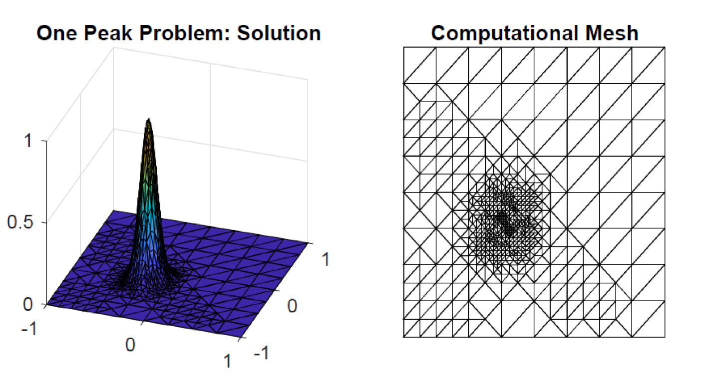
In our experiments we solve the simplified problem with $u=0$ on $\partial D$ . (This has no impact on accuracy for the error tolerances that we will considered; see the discussion in the appendix). The initial mesh with $81$ vertices is generated by taking three uniform refinement steps, starting from two triangles with common edge from $(-1,-1)$ to $(1,1)$ . For the specific parameter choice $y=(-0.22,-0.22)^{T}$ and spatial tolerance ${\eta_{X}}=2\times 10^{-3}$ , the adaptive algorithm terminated after 5 steps giving the numerical solution and corresponding mesh shown in Fig. 1.

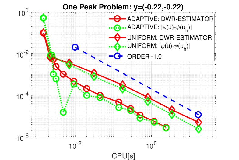
Running the adaptive algorithm with a tighter tolerance of ${\eta_{X}}=5\times 10^{-6}$ generated a concentrated mesh with $158\,734$ points after 13 refinement steps. The left part of Fig. 2 shows the efficiency of the locally adaptive procedure in comparison with a uniform refinement strategy. For smaller tolerances, the gain of efficiency in terms of overall cpu time is a factor $10$ . Comparing with a reference value $\psi(u)=0.025315675\ldots$ , generated by running the adaptive algorithm with a very small tolerance, we see that the effectivity index, i.e., the ratio between estimator and true error, tends asymptotically to $1$ for both uniform and adaptive refinement.

The very good quality of the spatial error estimation process is still maintained if we sample over the whole parameter space using an isotropic sparse grid of $145$ collocation points – generated using Sparse Grid Kit by doubling of points in each stochastic dimension. In this case we have a reference value of $\mathbb{E}[\psi(u)]=0.015095545\ldots$ , generated analytically using an asymptotic argument—details are given in the appendix. The error estimates for adaptive meshes associated with different spatial error tolerances are plotted in the right part of Fig. 2. Observe that the estimators deliver upper bounds for the numerical errors and the tolerances are always satisfied. As expected from the theory, the convergence rates for $\psi(u)$ and $\mathbb{E}[\psi(u)]$ in terms of computing time are both close to $-1$ . So we have $C_{X}\!=\!1$ in (30) and $s^{*}\!=\!1$ in assumption (A1) in Section 2.

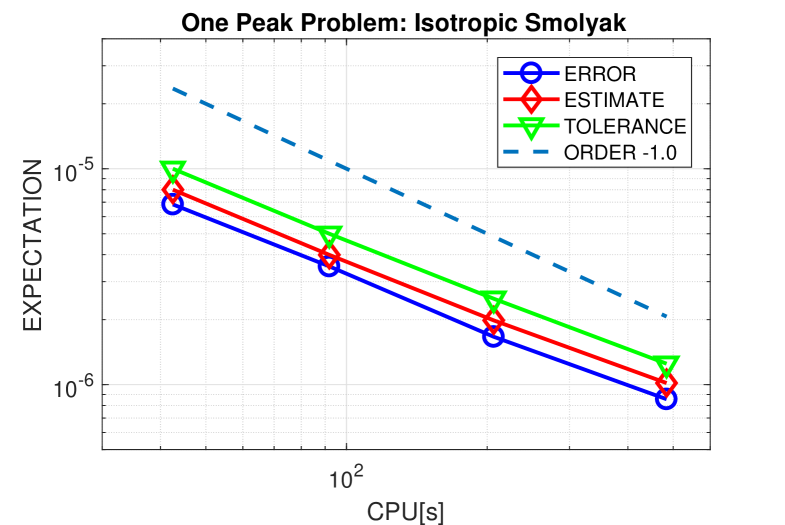
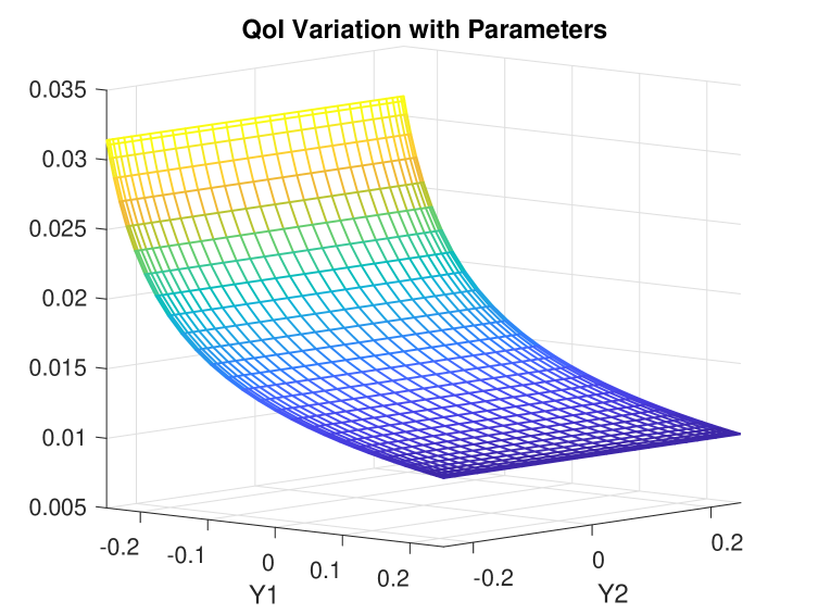
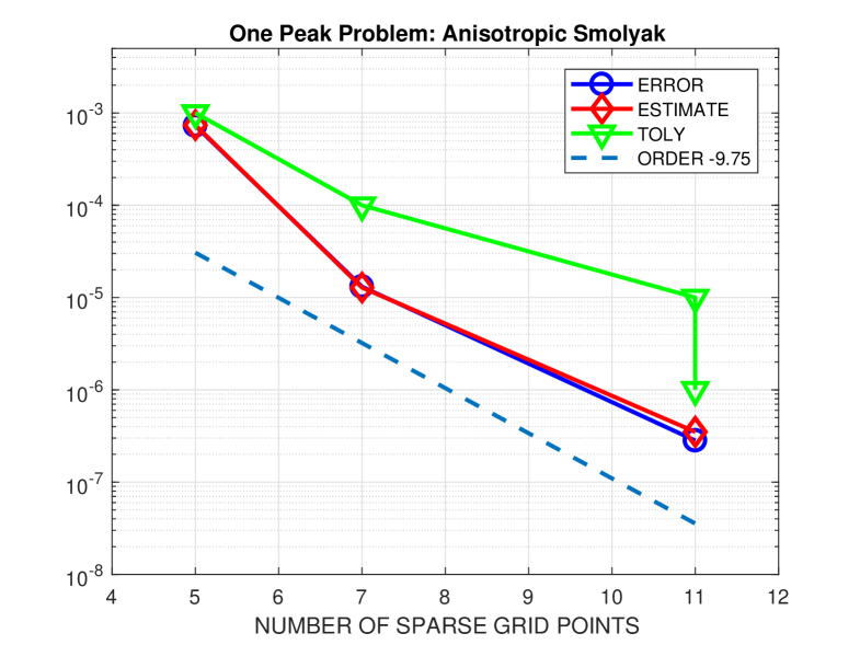
Next we consider the convergence behaviour and the quality of the error estimates for the adaptive anisotropic Smolyak algorithm. A reference solution generated by solving the problem with a small spatial error tolerance on a $33\times 33$ tensor-product grid of Clenshaw–Curtis points is shown in the left part of Fig. 3. Looking at the solution structure, it is evident that the QoI has inherent structure that can be exploited by an adaptive strategy: more specifically, very few sample points are needed to accurately compute it ! The right part of Fig. 3 shows the results for a decreasing sequence of stochastic tolerances ${\eta_{Y}}=10^{-3},\ldots,10^{-6}$ , where we have fixed the spatial tolerance ${\eta_{X}}=10^{-7}$ . The corresponding numbers of collocation points are $5,7,11$ , and $11$ . Looking at these more closely we find that all the quadrature rules generated by the adaptive procedure are one-dimensional rules in the $y_{1}$ direction matching the variation in the reference. Other features of note are that the prescribed tolerances are always satisfied and that the errors (with respect to the reference solution) are nicely estimated by the error indicators. A least-squares fit gives an averaged value of $\mu^{*}=9.75$ for the convergence order so that assumption (A2) in Section 2 is satisfied. An approximate value $\mu^{*}\approx 10.74$ can be computed with a much lower spatial tolerance $\eta_{X}=1.25\times 10^{-4}$ and $19$ collocation points in a few seconds.

Having estimated the parameters in the second step of the algorithm in Table 1, we now run the adaptive multilevel approach with overall accuracy requirements of $\epsilon=10^{-5},5\times 10^{-6},2.5\times 10^{-6}$ and $10^{-6}$ . To illustrate the performance gains, we simply set $K\!=\!2$ (so that three levels are used) and assign a spatial error reduction factor of $q=0.2$ . The spatial tolerances are then given by ${\eta_{X_{k}}}=\epsilon q^{k-2}/2$ with $k=0,1,2$ . To calculate, in a first step, a sufficiently accurate approximation for the tolerance ${\eta_{X_{-1}}}=\mathbb{E}[\psi(u_{0})]$ at reasonable cost, we apply the anisotropic Smolyak algorithm with ${\eta_{X}}={\eta_{Y}}={\eta_{X_{0}}}$ . Note that these samples can be reused later in the first level of the multilevel scheme. Eventually, the stochastic tolerances are derived from (22) with $C_{Y}=0.1$ , $\mu^{*}=9.75$ and $s^{*}=1$ .

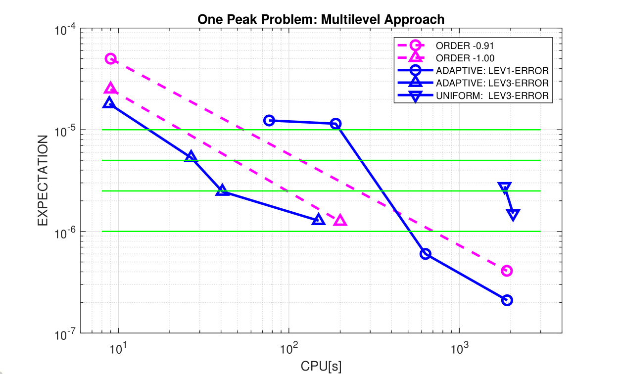
Results for the three-level and single-level approach are summarised in Fig. 4. For adaptive spatial meshes, we observe that the errors of the expected values $\mathbb{E}[\psi_{2}^{(\mathrm{ML})}]$ are very close to the prescribed tolerances. This is not always the case for the values $\mathbb{E}[\psi_{2}^{(\mathrm{SL})}]$ computed by the single-level approach. The three-level approach performs reliably and outperforms the single-level version clearly. The orders of convergence, $p_{\mathrm{ML}}\!=\!-1/s^{*}\!=\!-1$ and $p_{\mathrm{SL}}\!=\!-1/(s^{*}+1/{\mu^{*}})\!\approx\!-0.91$ , predicted by Theorem 2.1 for the accuracy in terms of computational complexity are also visible. Already for coarse tolerances, the three-level approach with uniform spatial meshes shown plotted with inverted blue triangles) is not competitive. For higher tolerances, the calculation exceeded memory requirements (more than $1.6\times 10^{7}$ FE degrees of freedom).

These CPU timings are impressive. We have also solved the one peak test problem using an efficient adaptive stochastic Galerkin (SG) approximation strategy. While the linear algebra associated with the Galerkin formulation is decoupled in this case, the computational overhead of evaluating the right-hand-side vector is a big limiting factor in terms of the relative efficiency. Using SG the quantity

I=\int_{\triangle}\int_{\Gamma}d({{x}},y)\cdot f({{x}},y)\,\psi_{\nu_{k}}(y)\,\phi_{j}({{x}})\,dy\,d{x}

where

f({{x}},y)=d(x_{1},x_{2},y_{1},y_{2})\cdot\exp(-50\{\alpha(y_{1})(x_{1}-y_{1})^{2}+(x_{2}-y_{2})^{2}\}),

and

d(x_{1},x_{2},y_{1},y_{2})=-10000\left\{\alpha^{2}(y_{1})(x_{1}-y_{1})^{2}+(x_{2}-y_{2})^{2}\right\}+100(\alpha(y_{1})+1)

must be computed in every element $\triangle$ in the current subdivision and for every parametric function $\psi_{\nu_{k}}(y)$ in the active index set. This is an extremely demanding quadrature problem!

We have also tested an adaptive multilevel Monte Carlo method (see, [12, 27]) on this problem. For the lowest tolerance, $\epsilon=10^{-5}$ , and an average over $5$ independent realizations, the three-level algorithm achieves an accuracy of $2.77\times 10^{-6}$ in $7.76\times 10^{4}$ sec. The numbers of averaged samples for each level are $M_{0}=519634$ , $M_{1}=6153$ , and $M_{2}=243$ . Obviously, the slow Monte Carlo convergence rate of $\mu=0.5$ is prohibitive for higher tolerances here.

3.2 Uncertain geometry: $d=2$ , $N=16$

In our second example, we again consider a two-dimensional Poisson problem, but now with geometry of the computational domain being uncertain. We will refer to this example as the two hole test problem. The uncertain domain is defined by

D(y)=(0,6)\times(0,6)\backslash(D_{1}(y)\cup D_{2}(y)),

(45)

where the holes $D_{1}(y)=\overline{P_{1}P_{2}P_{3}P_{4}}$ and $D_{2}(y)=\overline{P_{5}P_{6}P_{7}P_{8}}$ are taken as quadrilaterals with the uncertain vertices

\begin{array}[]{ll}P_{1}=(1+y_{1}/a_{1},1+y_{2}/a_{2}),&P_{2}=(2+y_{3}/a_{3},1+y_{4}/a_{4}),\\[2.84526pt] P_{3}=(2+y_{5}/a_{5},3+y_{6}/a_{6}),&P_{4}=(1+y_{7}/a_{7},3+y_{8}/a_{8}),\\[2.84526pt] P_{5}=(4+y_{9}/a_{9},1+y_{10}/a_{10}),&P_{6}=(5+y_{11}/a_{11},1+y_{12}/a_{12}),\\[2.84526pt] P_{7}=(5+y_{13}/a_{13},5+y_{14}/a_{14}),&P_{8}=(4+y_{15}/a_{15},5+y_{16}/a_{16}).\end{array}

(46)

Here, the random vector $y=(y_{1},\ldots,y_{16})^{T}$ consists of sixteen uniformly distributed random variables $y_{i}\sim{\cal U}[-1,1]$ , $i=1,\ldots,16$ . We set

(a_{1},\ldots,a_{16})=(5,5,5,5,5,5,5,5,10,10,10,10,20,20,20,20)

(47)

to represent different strength of uncertainty and hence anisotropy in the stochastic space. We impose a constant volume force $f\!\equiv\!1$ and fix the component by homogeneous Dirichlet boundary conditions on the whole boundary $\partial D(y)$ , including $\partial D_{1}(y)\cup\partial D_{2}(y)$ with stochastically varying positions in space. Our goal is then to study the effect of this uncertainty on the expectation of the overall displacement calculated by

\mathbb{E}[\psi(u,y)]=\mathbb{E}\left[\int_{D(y)}u^{2}(x,y)\,dx\right].

(48)

This allows an assessment of the desired averaged load capacity of the component, which takes into account uncertainties in the manufacturing process.

Applying a parameter-dependent map, each domain $D(y)$ can be mapped to the fixed nominal domain $D_{0}=D(0)$ with $0\in\mathbb{R}^{16}$ . Such a domain mapping approach was introduced by Xiu & Tartakovsky [38] and allows us to reformulate the problem in the form (1) with parameter-dependent coefficients on $D_{0}$ . The well established theory for elliptic partial differential equations with random input data can then be applied without modifications to show the well-posedness of the setting with random domains.

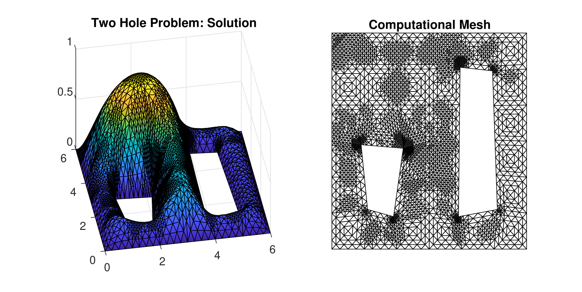
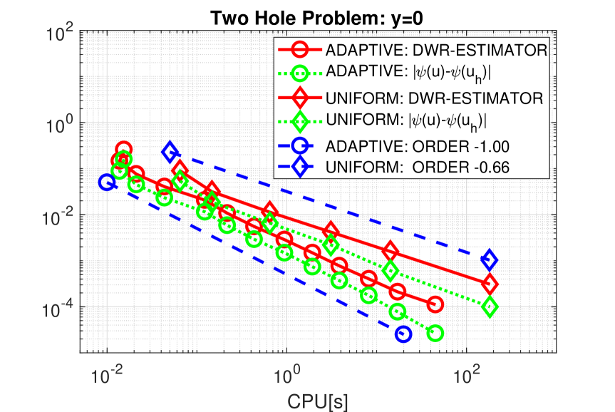
All calculations start with an initial criss-cross structured mesh consisting of $1920$ triangles, which are adjusted to the random holes. In Fig. 5, the numerical solution and its corresponding adaptive mesh for a spatial tolerance ${\eta_{X}}=10^{-1}$ and the random vector $y\!=\!(0.5,0.5,-0.5,-0.5,-0.5,-0.5,1,-1,-1,-1,1,1,-1,1,-1,-1)^{T}$ are shown. The adaptive algorithm refines the mesh at the eight reentrant corners due to the fact that the exact solution contains a loss of regularity there. Exemplarily, we study the convergence rates of adaptive and uniform refinements for the nominal domain $D_{0}$ , where $u(0)$ is contained in $H^{5/3}(D_{0})$ . While the correctly adapted grids still recover the optimal order $-1$ for the approximation of $\psi(u(0))$ in terms of CPU time, the use of a sequence of uniform meshes sees the order drop down to the theoretical value $-0.66$ , as can be seen in the left part of Fig. 6. The DWR-estimators perform quite well and deliver accurate upper bounds of the error. So we again set $C_{X}=1$ in (30) and use $s^{*}\!=\!1$ for adaptive meshes and $s^{*}=1.6$ for uniform meshes in assumption (A1). Note that the latter choice takes into account that due to the larger interior angle at the random holes for some parameter values $y\not=0$ , the regularity of the solution, and thus also the spatial convergence rate, is slightly lower.

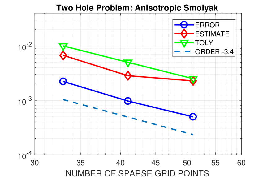
In order to estimate the parameter $\mu^{*}$ , we apply the anisotropic Smolyak algorithm and calculate samples at reasonable costs with tolerances ${\eta_{X}}={\eta_{Y}}=10^{-2}/2^{i},i=0,\ldots,3$ . The value of $\mathbb{E}[\psi(u)]$ for $i=3$ is taken as the reference value, leading to an approximate convergence order of $\mu^{*}=3.4$ . From Fig. 6, we detect that the errors are significantly smaller than the prescribed tolerances, as it was also the case in the first test example. Therefore, we again choose $C_{Y}=0.1$ and set $\mu^{*}=3.4$ in assumption (A2). For later comparison, we compute a reference value $\mathbb{E}[\psi(u)]=4.758057\ldots$ with ${\eta_{X}}=10^{-4}$ and ${\eta_{Y}}=5\times 10^{-4}$ . The required number of collocation points is $233$ and the vector of maximum polynomial degree is $(3\,2\,3\,3\,3\,3\,3\,3\,3\,3\,2\,2\,3\,2\,2\,2)^{T}$ .

For the adaptive multilevel approach, we use again three levels and set the reduction factor to $q=0.2$ . The spatial tolerances are then computed from ${\eta_{X_{k}}}=\epsilon q^{k-2}/2$ , $k=0,1,2$ , with the six overall accuracy requirements $\epsilon=10^{-2},5\times 10^{-3},2.5\times 10^{-3},10^{-3},5\times 10^{-4},2.5\times 10^{-4}$ . Following the algorithm given in Table 1, we first compute ${\eta_{X_{-1}}}=\mathbb{E}[\psi(u_{0})]$ with ${\eta_{X}}={\eta_{Y}}={\eta_{X_{0}}}$ and then derive the stochastic tolerances ${\eta_{Y_{k}}}$ from (22) with $C_{Y}=0.1$ , $\mu^{*}=3.4$ , and $s^{*}=1$ . The corresponding values are given in Table 2. For the multilevel approach with uniform spatial meshes, we use $s^{*}=1.6$ to determine the stochastic tolerances.

$\epsilon$	$10^{-2}$	$5\times 10^{-3}$	$2.5\times 10^{-3}$	$10^{-3}$	$5\times 10^{-4}$	$2.5\times 10^{-4}$
${\eta_{X_{-1}}}$	$4.7125$	$4.7346$	$4.7465$	$4.7525$	$4.7554$	$4.7566$
${\eta_{X_{0}}}$	$1.3\times 10^{-1}$	$6.3\times 10^{-2}$	$3.1\times 10^{-2}$	$1.3\times 10^{-2}$	$6.3\times 10^{-3}$	$3.1\times 10^{-3}$
${\eta_{X_{1}}}$	$2.5\times 10^{-2}$	$1.3\times 10^{-2}$	$6.3\times 10^{-3}$	$2.5\times 10^{-3}$	$1.3\times 10^{-3}$	$6.3\times 10^{-4}$
${\eta_{X_{2}}}$	$5.0\times 10^{-3}$	$2.5\times 10^{-3}$	$1.3\times 10^{-3}$	$5.0\times 10^{-4}$	$2.5\times 10^{-4}$	$1.3\times 10^{-4}$
${\eta_{Y_{2}}}$	$7.2\times 10^{-3}$	$4.1\times 10^{-3}$	$2.3\times 10^{-3}$	$1.1\times 10^{-3}$	$6.2\times 10^{-4}$	$3.5\times 10^{-4}$
${\eta_{Y_{1}}}$	$1.3\times 10^{-2}$	$6.1\times 10^{-3}$	$3.0\times 10^{-3}$	$1.1\times 10^{-3}$	$5.5\times 10^{-4}$	$2.6\times 10^{-4}$
${\eta_{Y_{0}}}$	$3.0\times 10^{-2}$	$1.5\times 10^{-2}$	$7.2\times 10^{-3}$	$2.8\times 10^{-3}$	$1.3\times 10^{-3}$	$6.4\times 10^{-4}$
$M_{0}$	$35$	$51$	$65$	$131$	$161$	$321$
$M_{1}$	$33$	$33$	$33$	$33$	$33$	$33$
$M_{2}$	$33$	$33$	$33$	$33$	$33$	$33$

Table 2: Adaptive multilevel collocation method: Sequences of spatial and stochastic tolerances,

{\eta_{X_{k}}}

and

{\eta_{Y_{k}}}

, for overall tolerances

\epsilon=10^{-2},\ldots,2.5\times 10^{-4}

and certain approximations of

{\eta_{X_{-1}}}

(above). Number of collocation points taken by the anisotropic Smolyak algorithm for

K\!=\!2

(below).

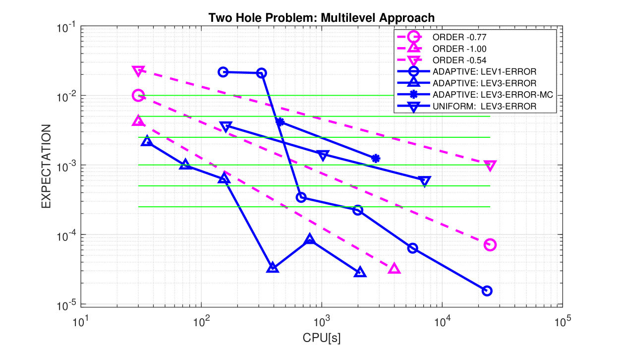
In Fig. 7, errors for the expected value $\mathbb{E}[\psi_{2}^{(\mathrm{ML})}]$ versus computing time are plotted for the three-level approach with adaptive and uniform spatial meshes. For comparison, we also show results for the single-level approach with adaptive spatial meshes, computed with ${\eta_{X}}=\epsilon/2$ and ${\eta_{Y}}=\epsilon/(2C_{Y})$ . In all cases, except the first two for the single-level method, the overall tolerances are satisfied. The schemes work remarkably reliably. However, the achieved accuracy is often significantly better than the prescribed one – never more than a factor $10$ though. One possible reason could be that cancellation effects are typically overlooked if the overall error is split into two parts, which are then individually controlled.

The multilevel method with adaptive spatial meshes outperforms the single-level approach. The number of collocation points taken by the anisotropic Smolyak algorithm are listed in Table 2. We observe that the number of samples for the differences keeps constant, showing that the increasing samples in the zeroth level always catch enough information to eventually reach the tolerance. The corresponding numbers of collocation points for the single-level method are $(1,1,33,41,51,105)$ . Note that the computing time also includes the effort for the estimation process, which is not visible in these numbers; see also the discussion for our realization of the adaptive anisotropic Smolyak algorithm above. It is also clear that the averaged constant $C_{Y}=0.1$ is too optimistic for the first runs with $\epsilon=10^{-2},5\times 10^{-3}$ , which leads to the algorithm taking only one collocation point. The approximate orders of convergence for both methods, $p_{\mathrm{ML}}=-1/s^{*}=-1$ and $p_{\mathrm{SL}}=-1/(s^{*}+1/\mu^{*})\approx-0.77$ , predict the observed asymptotic rates for the computing times quite well. However, the actual estimates can only serve as rough indicators for the achieved accuracy.

The multilevel method with uniform spatial meshes performs better than the single-level one for the first two tolerances, but becomes quickly inefficient for higher tolerances. Due to the larger value $s^{*}=1.6$ , it needs significantly more samples for coarser meshes: $M_{0}=(65,131,567)$ and $M_{1}=(33,33,105)$ , compared to the multilevel approach with adaptive spatial meshes, see Table 2. $M_{2}$ remains the same. The observed convergence order $-0.54$ is close to the predicted value $-1/s^{*}=-0.625$ . Also for this example, it becomes obvious that uniform meshes cannot compete with adaptive meshes for higher tolerances.

This conclusion is also valid for tests with adaptive multilevel Monte Carlo. Results for tolerances $\epsilon=10^{-2},5\times 10^{-3}$ are shown in Fig. 7 for three levels. The numbers of optimized samples are $M_{0}=(4140,17013)$ , $M_{1}=(48,108)$ , $M_{2}=(5,6)$ , respectively. All values are calculated from an average over 5 independent realizations. Although the variance reduction is quite high, leading to surprisingly small numbers $M_{2}$ , the fast increasing numbers for $M_{0}$ are still too challenging, especially for higher tolerances.

4 Concluding remarks

Adaptive methods have the potential to drastically reduce the number of degrees of freedom and to realise optimal complexity in terms of computing time, even in cases where the exact solutions have spatial singularities. As well as providing a posteriori error estimates, adaptive methods usually outperform methods based on uniform mesh refinement. When coupled with multilevel stochastic algorithms, they can increase the computational efficiency in the sampling process when the stochastic dimension increases and hence provide a general tool to further delay the curse of dimensionality.

State-of-the-art adaptive methods implemented in the open-source Matlab packages p1afem and Sparse Grid Kit have been used in off-the-shelf fashion in this study. The numerical results for the adaptive multilevel collocation method demonstrate the reliability of the error control and a significant decrease in complexity compared to uniform spatial refinement methods and single-level stochastic sampling methods. While these advantages are already known for the methods involved, this study shows that the adaptive components can be combined to give an efficient algorithm for solving PDEs with random data to arbitrary levels of accuracy.

Appendix.

The pathwise solution of the one peak problem is given by

u({{x}},y)=\exp(-\beta\{\alpha(y_{1})(x_{1}-y_{1})^{2}+(x_{2}-y_{2})^{2}\}),

(A ​ .1)

with $\alpha(y_{1})=18y_{1}+11/2$ . The quantity of interest is given by

\mathbb{E}\left[\phi(u)\right]=\int_{\Gamma}\int_{D}u^{2}({x},y)\rho(y)\,d{x}\,dy.

(A ​ .2)

The specific choice $\beta=50$ taken in the numerical experiments leads to two simplifications.

(S1)

The Dirichlet boundary condition ( $u$ satisfying (A.1) on $\partial D$ ) may be replaced without significant loss of accuracy by the numerical approximation

$u_{h}=0\hbox{ on }\partial D.$ $(A .3)$

Justification: By direct computation, the maximum value of $u$ on the boundary occurs for $\alpha=1$ , when the standard deviation $\sigma$ of the Gaussian peak is minimised (thus $\sigma_{*}=1/10$ and $y=(-1/4,y_{2})$ for all values $-1/4\leq y_{2}\leq 1/4$ ). For all such values of $y_{2}$ the nearest point on the boundary is ${{x}}=(-1,y_{2})$ , and the shortest distance to the boundary is $d=3/4$ so that the maximum value of $u$ on the boundary is given by $u_{\max}=\exp\big{(}-\frac{9\beta}{16}\big{)}\approx 6\cdot 10^{-13}$ .

(S2)

Thus, we may readily compute a reference value (accurate to more than 10 digits):

\mathbb{E}\left[\phi(u)\right]\approx Q:={1\over 9}\cdot(\sqrt{10}-1)\cdot{\pi\over\beta}=0.015095545\ldots

Justification: the integral in (A.2) is separable, thus

	$\displaystyle I$	$\displaystyle=\int_{\Gamma}\int_{D}u^{2}({x},y)\rho(y)\,d{x}\,dy$
		$\displaystyle=\int_{\Gamma}\int_{D}e^{-2\beta\{\alpha(x_{1}-y_{1})^{2}+(x_{2}-y_{2})^{2}\}}\rho(y)\,d{x}\,dy$
		$\displaystyle=\int_{-{1\over 4}}^{1\over 4}\hat{\rho}(y_{1})\int_{-1}^{1}e^{-2\beta\alpha(x_{1}-y_{1})^{2}}\,dx_{1}\,dy_{1}\cdot\int_{-1/4}^{1/4}\hat{\rho}(y_{2})\int_{-1}^{1}e^{-2\beta(x_{2}-y_{2})^{2}}\,dx_{2}\,dy_{2}.$

The key point is that the inner integrals in the above expression are Gaussians with small variance. In both cases the integrand is close to zero at the end points $-1$ and $1$ . Thus, in both cases the integral can be extended by zero to the range $(-\infty,\infty)$ (this could be made rigorous using probabilistic arguments) to give the following reference value approximation

	$\displaystyle Q$	$\displaystyle=\int_{-{1\over 4}}^{1\over 4}2\int_{-\infty}^{\infty}e^{-2\beta\alpha(x_{1}-y_{1})^{2}}\,dx_{1}\,dy_{1}\cdot\int_{-1/4}^{1/4}2\int_{-\infty}^{\infty}e^{-2\beta(x_{2}-y_{2})^{2}}\,dx_{2}\,dy_{2}$
		$\displaystyle=4\int_{-{1\over 4}}^{1\over 4}\sqrt{\pi\over 2\alpha\beta}\,dy_{1}\cdot\int_{-1/4}^{1/4}\sqrt{\pi\over 2\beta}\,dy_{2}$
		$\displaystyle={2\pi\over\beta}\int_{-1/4}^{1/4}\,dy_{2}\cdot\int_{-{1\over 4}}^{1\over 4}\alpha(y_{1})^{-1/2}\,dy_{1}={\pi\over\beta}\cdot{1\over 18}\,\underbrace{\int_{1}^{10}\alpha^{-1/2}\,d\alpha}_{2(\sqrt{10}-1)}.$

Acknowledgements. The first author is supported by the Deutsche Forschungsgemeinschaft (DFG, German Research Foundation) within the collaborative research center TRR154 “Mathematical modeling, simulation and optimisation using the example of gas networks” (Project-ID 239904186, TRR154/2-2018, TP B01), the Graduate School of Excellence Computational Engineering (DFG GSC233), and the Graduate School of Excellence Energy Science and Engineering (DFG GSC1070). The second author was supported by the UK Engineering and Physical Sciences Research Council (EPSRC) under grant number EP/K031368/1. The third author was funded by a Romberg visiting scholarship at the University of Heidelberg in 2019. The authors would also like to thank the Isaac Newton Institute for Mathematical Sciences, Cambridge, for support and hospitality during the programme “Uncertainty quantification for complex systems: theory and applications” (Jan–Jul 2018), where the work on this paper was initiated.

References

[1] R. C. Almeida and J. T. Oden. Solution verification, goal-oriented adaptive methods for stochastic advection-diffusion problems. Comput. Methods Appl. Mech. Engrg., 199:2472–2486, 2010.
[2] I. Babuška, F. Nobile, and R. Tempone. A stochastic collocation method for elliptic partial differential equations with random input data. SIAM J. Numer. Anal., 45:1005–1034, 2007.
[3] M. Bachmayr, A. Cohen, D. Dũng, and C. Schwab. Fully discrete approximation of parametric and stochastic elliptic PDEs. SIAM J. Numer. Anal., 55:2151–2186, 2017.
[4] A. Barth, C. Schwab, and N. Zollinger. Multi-level Monte Carlo finite element method for elliptic PDEs with stochastic coefficients. Numer. Math., 119:123–161, 2011.
[5] J. Beck, F. Nobile, L. Tamellini, and R. Tempone. Stochastic spectral Galerkin and collocation methods for PDEs with random coefficients: a numerical comparison. In J.S. Hesthaven and E.M. Ronquist, editors, Spectral and High Order Methods for PDEs, volume 76 of Lecture Notes Comput. Sci. Engrg., pages 43–62. Springer, 2011.
[6] R. Becker and R. Rannacher. An optimal control approach to a posteriori error estimation in finite element methods. Acta Numerica, 10:1–102, 2001.
[7] A. Bespalov, C. Powell, and D. Silvester. Energy norm a posteriori error estimation for parametric operator equations. SIAM J. Sci. Comput., 36:A339–A363, 2014.
[8] A. Bespalov, D. Praetorius, L. Rocchi, and M. Ruggeri. Goal-oriented error estimation and adaptivity for elliptic PDEs with parametric or uncertain inputs. Comp. Methods Appl. Mech. Engrg., 345:951–982, 2019.
[9] A. Bespalov and D. Silvester. Efficient adaptive stochastic Galerkin methods for parametric operator equations. SIAM J. Sci. Comput., 38:A2118–A2140, 2016.
[10] Alex Bespalov, Leonardo Rocchi, and David Silvester. T-IFISS: a toolbox for adaptive FEM computation. arXiv Preprint 1908.05618, 2019. https://arxiv.org/abs/1908.05618.
[11] A. Chkifa, A. Cohen, and C. Schwab. High-dimensional adaptive sparse polynomial interpolation and applications to parametric PDEs. Found. Comput. Math., 14:601–633, 2014.
[12] K.A. Cliffe, M.B. Giles, R. Scheichl, and A.L. Teckentrup. Multilevel Monte Carlo methods and applications to elliptic PDEs with random coefficients. Comput. Visual. Sci., 14:3–15, 2011.
[13] A. Cohen, A. Chkifa, C. Schwab, and R. Devore. Sparse adaptive Taylor approximation algorithms for parametric and stochastic PDE’s. ESAIM–Math. Model. Num., 47(1):253–280, 2013.
[14] G. Detommaso, T. Dodwell, and R. Scheichl. Continuous level Monte Carlo and sample-adaptive model hierarchies. SIAM/ASA J. Uncertain., 7:93–116, 2019.
[15] W. Dörfler. A convergent adaptive algorithm for Poisson’s equation. SIAM J. Numer. Anal., 33:1106–1124, 1996.
[16] M. Eigel, C. Gittelsson, C. Schwab, and E. Zander. Adaptive stochastic Galerkin FEM. Comput. Methods Appl. Mech. Engrg., 270:247 – 269, 2014.
[17] M. Eigel, C. Gittelsson, C. Schwab, and E. Zander. A convergent adaptive stochastic Galerkin finite element method with quasi-optimal spatial meshes. ESAIM–Math. Model. Num., 49(5):1367–1398, 2015.
[18] M. Eigel, Ch. Merdon, and J. Neumann. An adaptive Monte Carlo method with stochastic bounds for quantities of interest with uncertain data. SIAM/ASA J. Uncertain., 4:1219–1245, 2016.
[19] D. Elfverson, F. Hellman, and A. Målqvist. A multilevel Monte Carlo method for computing failure probablities. SIAM/ASA J. Uncertain., 4:312–330, 2016.
[20] S. Funken, D. Praetorius, and P. Wissgott. Efficient implementation of adaptive P1-FEM in Matlab, software available at http://www.asc.tuwien.ac.at/~praetorius/matlab.
[21] S. Funken, D. Praetorius, and P. Wissgott. Efficient implementation of adaptive P1-FEM in Matlab (extended preprint). ASC Report 19/2008, Vienna University of Technology, 2008.
[22] S. Funken, D. Praetorius, and P. Wissgott. Efficient implementation of adaptive P1-FEM in Matlab. Comput. Meth. Appl. Math., 11:460–490, 2011.
[23] T. Gerstner and M. Griebel. Dimension-adaptive tensor-product quadrature. Computing, 71:65–87, 2003.
[24] M. Giles. Multilevel Monte Carlo path simulation. Operations Res., 56:607–617, 2008.
[25] D. Guignard and F. Nobile. A posteriori error estimation for the stochastic collocation finite element method. SIAM J. Numer. Anal., 56(5):3121–3143, 2018.
[26] S. Heinrich. Multilevel Monte Carlo methods. In S. Margenov, J. Waniewski, and P. Yalamov, editors, Large-Scale Scientific Computing, volume 2179 of Lecture Notes Comput. Sci., pages 58–67. Springer, 2001.
[27] R. Kornhuber and E. Youett. Adaptive multilevel Monte Carlo methods for stochastic variational inequalities. SIAM J. Numer. Anal., 56:1987–2007, 2018.
[28] C. Kreuzer and K.G. Siebert. Decay rates of adaptive finite elements with Dörfler marking. Numer. Math., 1147:679–716, 2011.
[29] F. Nobile, L. Tamellini, and R. Tempone. Convergence of quasi-optimal sparse-grid approximation of Hilbert-space-valued functions: application to random elliptic PDEs. Numer. Math., 134:343–388, 2016.
[30] F. Nobile, L. Tamellini, F. Tesei, and R. Tempone. An adaptive sparse grid algorithm for elliptic PDEs with lognormal diffusion coefficient. In J. Garcke and D. Pflüger, editors, Sparse Grids and Applications—Stuttgart 2014, pages 191–220. Springer, 2016.
[31] F. Nobile, R. Tempone, and C. Webster. An anisotropic sparse grid stochastic collocation method for partial differential equations with random input data. SIAM J. Numer. Anal., 46:2411–2442, 2008.
[32] F. Nobile, R. Tempone, and C. Webster. A sparse grid stochastic collocation method for partial differential equations with random input data. SIAM J. Numer. Anal., 46:2309–2345, 2008.
[33] B. Schieche and J. Lang. Adjoint error estimation for stochastic collocation methods. In J. Garcke and D. Pflüger, editors, Sparse Grids and Applications—Munich 2012, volume 97 of Lecture Notes Comput. Sci. Engrg., pages 271–294. Springer, 2014.
[34] L. Tamellini, F. Nobile, D. Guignard, F. Tesei, and B. Sprungk. Sparse grid matlab kit, version 17-5, software available at https://csqi.epfl.ch.
[35] A.L. Teckentrup. Multilevel Monte Carlo Methods and Uncertainty Quantication. PhD thesis, University of Bath, 2013.
[36] A.L. Teckentrup, P. Jantsch, C.G. Webster, and M. Gunzburger. A multilevel stochastic collocation method for partial differential equations with random input data. SIAM/ASA J. Uncertain., 3:1046–1074, 2015.
[37] D. Xiu and J. S. Hesthaven. High-order collocation methods for differential equations with random inputs. SIAM J. Sci. Comput., 27:1118–1139, 2005.
[38] D. Xiu and D. Tartakovsky. Numerical methods for differential equations in random domains. SIAM J. Sci. Comput., 28:1167–1185, 2007.
[39] E. Youett. Adaptive Multilevel Monte Carlo Methods for Random Elliptic Problems. PhD thesis, Freie Universität Berlin, 2018.
[40] J. Zech. Sparse-Grid Approximation of High-Dimensional Parametric PDEs. PhD thesis, ETH Zürich, 2018.
[41] J. Zech, D. Dũng, and C. Schwab. Multilevel approximation of parametric and stochastic pdes. SAM Research Report 2018–05, ETH, Zurich, 2018. https://www.sam.math.ethz.ch/sam_reports/reports_final/reports2018/2018-05.pdf.