This paper was converted on www.awesomepapers.org from LaTeX by an anonymous user.
Want to know more? Visit the Converter page.

A General Approach for Parisian Stopping Times under Markov Processes

Gongqiu Zhang School of Science and Engineering, The Chinese University of Hong Kong, Shenzhen, China. Email: zhanggongqiu@cuhk.edu.cn.    Lingfei Li Corresponding author. Department of Systems Engineering and Engineering Management, The Chinese University of Hong Kong, Hong Kong SAR. Email: lfli@se.cuhk.edu.hk.
(July 26, 2025)
Abstract

We propose a method based on continuous time Markov chain approximation to compute the distribution of Parisian stopping times and price Parisian options under general one-dimensional Markov processes. We prove the convergence of the method under a general setting and obtain sharp estimate of the convergence rate for diffusion models. Our theoretical analysis reveals how to design the grid of the CTMC to achieve faster convergence. Numerical experiments are conducted to demonstrate the accuracy and efficiency of our method for both diffusion and jump models. To show the versality of our approach, we develop extensions for multi-sided Parisian stopping times, the joint distribution of Parisian stopping times and first passage times, Parisian bonds and for more sophisticated models like regime-switching and stochastic volatility models.

Keywords: Parisian stopping time, Parisian options, Parisian ruin probability, Markov chain approximation, grid design.

MSC (2020) Classification: 60J28, 60J60, 91G20, 91G30, 91G60.

JEL Classification: G13.

1 Introduction

Consider a stochastic process XX and define

gL,t=sup{st:XsL},gL,t+=sup{st:XsL}.\displaystyle g^{-}_{L,t}=\sup\{s\leq t:X_{s}\geq L\},\ g^{+}_{L,t}=\sup\{s\leq t:X_{s}\leq L\}. (1.1)

for a given level LL. The ages of excursion of XX below and above LL are given by tgL,tt-g^{-}_{L,t} and tgL,t+t-g^{+}_{L,t}, respectively. Consider the following two stopping times:

τL,D+=inf{t0:1{Xt>L}(tgL,t+)D},τL,D=inf{t0:1{Xt<L}(tgL,t)D},\displaystyle\tau_{L,D}^{+}=\inf\{t\geq 0:1_{\{X_{t}>L\}}(t-g^{+}_{L,t})\geq D\},\ \tau_{L,D}^{-}=\inf\{t\geq 0:1_{\{X_{t}<L\}}(t-g^{-}_{L,t})\geq D\}, (1.2)

which are called Parisian stopping times. τL,D+\tau_{L,D}^{+} (τL,D\tau_{L,D}^{-}) is the first time that the age of excursion of XX above (below) LL reaches DD. In these definitions, we use the convention that sup=0\sup\emptyset=0 and inf=\inf\emptyset=\infty.

Parisian stopping times appear in important finance and insurance applications. Parisian options are proposed in Chesney et al. (1997) as an alternative to barrier options and they have the advantage of being less prone to market manipulation (Labart (2010)). These options are activated or cancelled if the process stays long enough below or above a prespecified level. In the insurance literature, the Parisian stopping time for the excursion below the solvency level is used to define the ruin event (e.g., Dassios and Wu (2008), Czarna and Palmowski (2011), Loeffen et al. (2013)).

There is an extensive literature on the study of Parisian stopping times and their applications in finance and insurance with many papers focused on specific models. For the Brownian motion and the geometric Brownian motion model, see Chesney et al. (1997), Bernard et al. (2005), Dassios and Wu (2010), Dassios and Wu (2011), Zhu and Chen (2013), Dassios and Lim (2013), Dassios and Zhang (2016), Le et al. (2016), Dassios and Lim (2017) and Dassios and Lim (2018). For models with jumps, methods for Parisian option pricing were developed in Albrecher et al. (2012) for Kou’s double-exponential jump-diffusion model and in Chesney and Vasiljević (2018) for the hyper-exponential jump-diffusion model. Czarna and Palmowski (2011) and Loeffen et al. (2013) derived the ruin probability for spectrally negative Lévy processes. In addition, Chesney and Gauthier (2006), Le et al. (2016) and Lu et al. (2018) studied American-style Parisian option pricing under the Black-Scholes model while Chesney and Vasiljević (2018) dealt with the hyper-exponential jump-diffusion model. As for the hedging of Parisian options, Kim and Lim (2016) developed a quasi-static strategy and tested it under the double-exponential jump-diffusion model.

Several numerical methods have also been applied to the Parisian option pricing problem. Baldi et al. (2000) developed a Monte Carlo simulation method based on large deviation estimates for general diffusions. For the Black-Scholes model, Avellaneda and Wu (1999) proposed a trinomial tree approach while Haber et al. (1999) developed an explicit finite difference scheme to numerically solve the pricing PDE, which is not unconditionally stable. These two methods can also be applied to general diffusions, but they need to incorporate the current length of excursion as an additional dimension. Furthermore, they may require a very small time step to achieve a target accuracy level, making them inefficient. If the model contains jumps, the lattice method and the finite difference approach will face more challenges for accuracy and efficiency.

In this paper, we aim to develop a computationally efficient approach for Parisian stopping time problems that is applicable to general Markov models. We consider a one-dimensional (1D) Markov process XX living on an interval II\subseteq\mathbb{R} with its infinitesimal generator 𝒢\mathcal{G} given by

𝒢f(x)=12σ2(x)f′′(x)+μ(x)f(x)+(f(x+z)f(x)z1{|z|1}f(x))ν(x,dz)\displaystyle\mathcal{G}f(x)=\frac{1}{2}\sigma^{2}(x)f^{\prime\prime}(x)+\mu(x)f^{\prime}(x)+\int_{\mathbb{R}}\left(f(x+z)-f(x)-z1_{\{|z|\leq 1\}}f^{\prime}(x)\right)\nu(x,dz) (1.3)

for fCc2(I)f\in C_{c}^{2}(I) (the space of twice continuously differentiable functions on II with compact support) with (z21)ν(x,dz)<\int_{\mathbb{R}}(z^{2}\wedge 1)\nu(x,dz)<\infty. The quantities μ(x)\mu(x), σ(x)\sigma(x), ν(x,dz)\nu(x,dz) are known as the drift, volatility and jump measure of XX, respectively. We would like to obtain the distribution of τL,D\tau_{L,D}^{-} and τL,D+\tau_{L,D}^{+}, i.e., x[τL,D±t]\mathbb{P}_{x}[\tau_{L,D}^{\pm}\leq t]. The Laplace transform of the probability as a function of tt is given by

0eqtx[τL,D±t]𝑑t=𝔼x[τL,D±eqt𝑑t]=1q𝔼x[eqτL,D±],(q)>0.\displaystyle\int_{0}^{\infty}e^{-qt}\mathbb{P}_{x}[\tau_{L,D}^{\pm}\leq t]dt=\mathbb{E}_{x}\left[\int_{\tau_{L,D}^{\pm}}^{\infty}e^{-qt}dt\right]=\frac{1}{q}\mathbb{E}_{x}\left[e^{-q\tau_{L,D}^{\pm}}\right],\ \Re(q)>0. (1.4)

For a general Markov process, there is no analytical solution for this transform. Our idea is approximating XX by a continuous time Markov chain (CTMC). We will show later that the Laplace transform of τL,D±\tau_{L,D}^{\pm} under a CTMC model is the solution to a linear system which involves the distribution and the Laplace transform of a first passage time of the CTMC, and this solution can be obtained in closed form. To recover the distribution of τL,D±\tau_{L,D}^{\pm}, we simply invert its Laplace transform numerically using the efficient algorithm of Abate and Whitt (1992). Using the result for τL,D±\tau_{L,D}^{\pm}, we can compute the Laplace transfrom of a Parisian option price as a function of maturity in closed form for a CTMC model. We can further solve a range of Parisian problems under a CTMC model such as the distribution of the multi-sided Parisian stopping time, the joint distribution of a Parisian stopping time and a first passage time and the pricing of Parisian bonds. For more complex models like regime-switching models and stochastic volatility models, we can also approximate them by a CTMC and solve the Parisian stopping time problems. Thus, our approach is very general and versatile. Numerical experiments for various popular models further demonstrate the computational efficiency of our method, which can outpeform traditional numerical methods significantly.

Our paper fits into a burgeoning literature on CTMC approximation for option pricing. Mijatović and Pistorius (2013) used it for pricing European and barrier options under general 1D Markov models. They showed that the barrier option price can be obtained in closed form using matrix exponentials under a CTMC model. Sharp converegnce rate analysis of their algorithm for realistic option payoffs is a challenging problem. Answers are provided for diffusion models first in Li and Zhang (2018) for uniform grids and then in Zhang and Li (2021a)) for general non-uniform grids while the problem still remains open for general Markov models with jumps. For diffusions, Zhang and Li (2021a) also developed principles for designing grids to achieve second order convergence whereas the algorithm only converges at first order in general. The idea of CTMC approximation has also been exploited to develop efficient methods for pricing various types of options for 1D Markov models: Eriksson and Pistorius (2015) for American options, Cai et al. (2015), Song et al. (2018), Cui et al. (2018) for Asian options, and Zhang and Li (2021b) and Zhang et al. (2021) for maximum drawdown options. Furthermore, CTMC approximation can be extended to deal with more complex models where the asset price follows a regime-switching process (Cai et al. (2019)) or exhibits stochastic volatility (Cui et al. (2017, 2018, 2019)).

One can view the present paper as a generalization of Mijatović and Pistorius (2013) and Zhang and Li (2019) from barrier options to Parisian options. However, this generalization is by no means trivial. First, the Parisian problem is much more complex than the first passage problem as it involves the excursion of the process. Second, there is considerable challenge in sharp convergence rate analysis. Even for barrier options, the sharp convergence rate of CTMC approximation is only known for diffusion models, and the difficulty mainly stems from the lack of smoothness in the option payoffs. In this paper, we focus on analyzing the convergence rate of our algorithm for Parisian problems under diffusion models. We use the spectral analysis framework in Zhang and Li (2021a), but there is an important difference which makes the analysis for Parisian problems much harder. Here, we must carefully analyze the dependence of solutions to Sturm-Liouville and elliptic boundary value problems on variable boundary levels whereas in the barrier option problem the boundaries are fixed. Furthermore, we need to establish some new identities that enable us to obtain the sharp rate. Our analysis not only yields the sharp estimate of the convergence rate, but also unveils how the grid of the CTMC should be designed to achieve fast convergence.

For the sake of simplicity, our discussions in the main text will be focused on the algorithms for single-barrier Parisian stopping times and the down-and-in Parisian option as well as their convergence analysis. Extensions for other cases are provided in the appendix. The rest of this paper is organized as follows. In Section 2, we derive the Laplace transforms of Parisian stopping times and Parisian option prices under a general CTMC model with finite number of states. Section 3 reviews how to construct a CTMC to approximate a general jump-diffusion and establishes the convergence of this approximation for the Parisian problems. Section 4 analyzes the convergence rate for diffusion models and proposes grid design principles to ensure second order convergence. Section 5 shows numerical results for various models and Section 6 concludes the paper. In Appendix A, we extend our method to deal with multi-sided Parisian stopping times, the joint distribution of Parisian stopping times and first passage times, Parisian bonds and the Parisian problem for regime-switching and stochastic volatility models. Proofs for the convergence rate analysis are collected in Appendix B.

2 Parisian Stopping Times Under a CTMC

Consider a CTMC denoted by YY which lives in the state space 𝕊n={y0,y1,,yn}\mathbb{S}_{n}=\{y_{0},y_{1},\cdots,y_{n}\}. The transition rate matrix of YY is denoted by 𝑮{\boldsymbol{G}} with 𝑮(x,y){\boldsymbol{G}}(x,y) indicating the transition rate from state xx to yy, xyx\neq y and 𝑮(x,x)=y𝕊n\{x}𝑮(x,y){\boldsymbol{G}}(x,x)=-\sum_{y\in\mathbb{S}_{n}\backslash\{x\}}{\boldsymbol{G}}(x,y). The action of 𝑮\boldsymbol{G} on a function g:𝕊ng:\mathbb{S}_{n}\to\mathbb{R} is defined as

𝑮g(x)=y𝕊n𝑮(x,y)g(y),x𝕊n.\displaystyle{\boldsymbol{G}}g(x)=\sum_{y\in\mathbb{S}_{n}}{\boldsymbol{G}}(x,y)g(y),\ x\in\mathbb{S}_{n}. (2.1)

For any ξ\xi, we also introduce the notations

ξ+=min{z>ξ:z𝕊n},forξ<yn,\displaystyle\xi^{+}=\min\{z>\xi:z\in\mathbb{S}_{n}\},\ \text{for}\ \xi<y_{n}, (2.2)
ξ=max{z<ξ:z𝕊n},forξ>y0,\displaystyle\xi^{-}=\max\{z<\xi:z\in\mathbb{S}_{n}\},\ \text{for}\ \xi>y_{0}, (2.3)

which are the CTMC states that are the right and left neighbor of ξ\xi, respectively. We also define L+=min{zL:z𝕊n}L^{+}=\min\{z\geq L:z\in\mathbb{S}_{n}\}. Note that L+L^{+} is different from ξ+\xi^{+} in that L+=LL^{+}=L if L𝕊nL\in\mathbb{S}_{n}, but we always have ξ+>ξ\xi^{+}>\xi. We slightly abuse the notation here to avoid introducing a new one.

In this section, we first derive the Laplace transform of Parisian stopping times and then the Laplace transform of the price of a down-and-in Parisian option.

2.1 Laplace Transform of Parisian Stopping Times

Define

hn(q,x;y):=𝔼x[eqτL,D1{YτL,D=y}],x,y𝕊n,\displaystyle h_{n}(q,x;y):=\mathbb{E}_{x}\left[e^{-q\tau_{L,D}^{-}}1_{\{Y_{\tau_{L,D}^{-}}=y\}}\right],\ x,y\in\mathbb{S}_{n}, (2.4)

which is the Laplace transform of τL,D\tau_{L,D}^{-} given Y0=xY_{0}=x with an indicator for the process landing on yy at τL,D\tau_{L,D}^{-}. The joint distribution of τL,D\tau_{L,D}^{-} and YτL,DY_{\tau_{L,D}^{-}} is characterized by h(q,x;y)h(q,x;y). We also define

hn(q,x):=y𝕊nhn(q,x;y)=𝔼x[eqτL,D],x𝕊n,\displaystyle h_{n}(q,x):=\sum_{y\in\mathbb{S}_{n}}h_{n}(q,x;y)=\mathbb{E}_{x}\left[e^{-q\tau_{L,D}^{-}}\right],\ x\in\mathbb{S}_{n}, (2.5)

which is the Laplace transform of τL,D\tau_{L,D}^{-} given Y0=xY_{0}=x. To calculate hn(q,x;y)h_{n}(q,x;y) and hn(q,x)h_{n}(q,x), we introduce the following quantities that involve the first passage times of YY:

τL+:=inf{t:YtL},τL:=inf{t:Yt<L},\displaystyle\tau_{L}^{+}:=\inf\{t:Y_{t}\geq L\},\ \tau_{L}^{-}:=\inf\{t:Y_{t}<L\}, (2.6)
vn(D,x;y):=𝔼x[1{τL+D}1{YD=y}],\displaystyle v_{n}(D,x;y):=\mathbb{E}_{x}\left[1_{\{\tau_{L}^{+}\geq D\}}1_{\{Y_{D}=y\}}\right], (2.7)
vn(D,x):=y𝕊vn(D,x;y)=𝔼x[1{τL+D}],\displaystyle v_{n}(D,x):=\sum_{y\in\mathbb{S}}v_{n}(D,x;y)=\mathbb{E}_{x}\left[1_{\{\tau_{L}^{+}\geq D\}}\right], (2.8)
un+(q,D,x;z):=𝔼x[eqτL+1{τL+<D}1{YτL+=z}],\displaystyle u^{+}_{n}(q,D,x;z):=\mathbb{E}_{x}\left[e^{-q\tau_{L}^{+}}1_{\{\tau_{L}^{+}<D\}}1_{\{Y_{\tau_{L}^{+}}=z\}}\right], (2.9)
un(q,x;z):=𝔼x[eqτL1{YτL=z}].\displaystyle u^{-}_{n}(q,x;z):=\mathbb{E}_{x}\left[e^{-q\tau_{L}^{-}}1_{\{Y_{\tau_{L}^{-}}=z\}}\right]. (2.10)
Remark 2.1.

Throughout the paper, the variable before the semicolon indicates the initial state and the variable after it indicates the state at a stopping time or fixed time.

Using the strong Markov property of YY, we can derive the following two equations for hn(q,x;y)h_{n}(q,x;y) and hn(q,x)h_{n}(q,x) using the first passage quantities.

Theorem 2.1.

For x𝕊nx\in\mathbb{S}_{n},

hn(q,x;y)\displaystyle h_{n}(q,x;y) =1{x<L}eqDvn(D,x;y)+1{x<L}zLun+(q,D,x;z)hn(q,z;y)\displaystyle=1_{\{x<L\}}e^{-qD}v_{n}(D,x;y)+1_{\{x<L\}}\sum_{z\geq L}u^{+}_{n}(q,D,x;z)h_{n}(q,z;y) (2.11)
+1{xL}z<Lun(q,x;z)hn(q,z;y),\displaystyle\quad+1_{\{x\geq L\}}\sum_{z<L}u^{-}_{n}(q,x;z)h_{n}(q,z;y), (2.12)
hn(q,x)\displaystyle h_{n}(q,x) =1{x<L}eqDvn(D,x)+1{x<L}zLun+(q,D,x;z)hn(q,z)\displaystyle=1_{\{x<L\}}e^{-qD}v_{n}(D,x)+1_{\{x<L\}}\sum_{z\geq L}u^{+}_{n}(q,D,x;z)h_{n}(q,z) (2.13)
+1{xL}z<Lun(q,x;z)hn(q,z).\displaystyle\quad+1_{\{x\geq L\}}\sum_{z<L}u^{-}_{n}(q,x;z)h_{n}(q,z). (2.14)
Proof.

First, consider the case x<Lx<L. We have

hn(q,x;y)=𝔼x[eqτL,D1{YτL,D=y}1{τL+D}]+𝔼x[eqτL,D1{YτL,D=y}1{τL+<D}].h_{n}(q,x;y)=\mathbb{E}_{x}\left[e^{-q\tau_{L,D}^{-}}1_{\{Y_{\tau_{L,D}^{-}}=y\}}1_{\{\tau^{+}_{L}\geq D\}}\right]+\mathbb{E}_{x}\left[e^{-q\tau_{L,D}^{-}}1_{\{Y_{\tau_{L,D}^{-}}=y\}}1_{\{\tau^{+}_{L}<D\}}\right]. (2.15)

The first term represents the case that YY does not cross LL from below by time DD. In this case, τL,D=D\tau_{L,D}^{-}=D and hence hn(q,x;y)=eqDvn(D,x;y)h_{n}(q,x;y)=e^{-qD}v_{n}(D,x;y), where vn(D,x;y)v_{n}(D,x;y) is the probability that the first time YY greater than or equal to LL exceeds DD and YD=yY_{D}=y.

The second term stands for the case that YY crosses LL from below before time DD. Using the strong Markov property, the process restarts at τL+\tau_{L}^{+} from YτL+Y_{\tau_{L}^{+}} and the clock tgL,tt-g_{L,t}^{-} is reset to zero. Thus, the second term becomes

zL𝔼x[eqτL+1{τL+<D}1{YτL+=z}𝔼[eqτL,D1{YτL,D=y}|τL+<D,YτL+=z]]\displaystyle\sum_{z\geq L}\mathbb{E}_{x}\left[e^{-q\tau_{L}^{+}}1_{\{\tau^{+}_{L}<D\}}1_{\{Y_{\tau_{L}^{+}}=z\}}\mathbb{E}\left[e^{-q\tau_{L,D}^{-}}1_{\{Y_{\tau_{L,D}^{-}}=y\}}\Big{|}\tau^{+}_{L}<D,Y_{\tau_{L}^{+}}=z\right]\right] (2.16)
=zL𝔼x[eqτL+1{τL+<D}1{YτL+=z}hn(q,z;y)]=zLun+(q,D,x;z)hn(q,z;y).\displaystyle=\sum_{z\geq L}\mathbb{E}_{x}\left[e^{-q\tau_{L}^{+}}1_{\{\tau^{+}_{L}<D\}}1_{\{Y_{\tau_{L}^{+}}=z\}}h_{n}(q,z;y)\right]=\sum_{z\geq L}u^{+}_{n}(q,D,x;z)h_{n}(q,z;y). (2.17)

Next, consider the case xLx\geq L. The clock tgL,tt-g_{L,t}^{-} would not tick until YY crosses LL from above, at which time the process restarts at YτLY_{\tau_{L}^{-}} by the strong Markov property and tgL,tt-g_{L,t}^{-} starts ticking. Thus, we have

hn(q,x;y)\displaystyle h_{n}(q,x;y) =z<L𝔼x[eqτL1{YτL=z}𝔼[eqτL,D1{YτL,D=y}|YτL=z]]\displaystyle=\sum_{z<L}\mathbb{E}_{x}\left[e^{-q\tau_{L}^{-}}1_{\{Y_{\tau_{L}^{-}}=z\}}\mathbb{E}\left[e^{-q\tau_{L,D}^{-}}1_{\{Y_{\tau_{L,D}^{-}}=y\}}\Big{|}Y_{\tau_{L}^{-}}=z\right]\right] (2.18)
=z<L𝔼x[eqτL1{YτL=z}hn(q,z;y)]=z<Lun(q,x;z)hn(q,z;y).\displaystyle=\sum_{z<L}\mathbb{E}_{x}\left[e^{-q\tau_{L}^{-}}1_{\{Y_{\tau_{L}^{-}}=z\}}h_{n}(q,z;y)\right]=\sum_{z<L}u^{-}_{n}(q,x;z)h_{n}(q,z;y). (2.19)

Putting these results together yields the equation for hn(q,x;y)h_{n}(q,x;y). The equation for hn(q,x)h_{n}(q,x) is obtained by summing the equation for hn(q,x;y)h_{n}(q,x;y) over yy. ∎

Solving (2.12) and (2.14) requires the quantities for first passage times, which we show are solutions to some equations.

Proposition 2.1.

We have the following equations for vn(D,x;y)v_{n}(D,x;y), un+(q,D,x;z)u^{+}_{n}(q,D,x;z) and un(q,x;z)u^{-}_{n}(q,x;z).

  1. 1.

    vn(D,x;y)v_{n}(D,x;y) satisfies

    {vnD(D,x;y)=𝑮vn(D,x;y),D>0,x𝕊n(,L),vn(D,x;y)=0,D>0,x𝕊n[L,),vn(0,x;y)=1{x=y},x𝕊n.\displaystyle\begin{cases}\frac{\partial v_{n}}{\partial D}(D,x;y)={\boldsymbol{G}}v_{n}(D,x;y),\ D>0,\ x\in\mathbb{S}_{n}\cap(-\infty,L),\\ v_{n}(D,x;y)=0,\ D>0,\ x\in\mathbb{S}_{n}\cap[L,\infty),\\ v_{n}(0,x;y)=1_{\{x=y\}},\ x\in\mathbb{S}_{n}.\end{cases} (2.20)
  2. 2.

    un+(q,D,x;z)u_{n}^{+}(q,D,x;z) satisfies

    {un+D(q,D,x;z)=(𝑮q𝑰)un+(q,D,x;z),D>0,x𝕊n(,L),un+(q,D,x;z)=1{x=z},D>0,x𝕊n[L,),un+(q,0,x;z)=0,x𝕊n.\displaystyle\begin{cases}\frac{\partial u^{+}_{n}}{\partial D}(q,D,x;z)=({\boldsymbol{G}}-q{\boldsymbol{I}})u^{+}_{n}(q,D,x;z),\ D>0,\ x\in\mathbb{S}_{n}\cap(-\infty,L),\\ u^{+}_{n}(q,D,x;z)=1_{\{x=z\}},\ D>0,\ x\in\mathbb{S}_{n}\cap[L,\infty),\\ u^{+}_{n}(q,0,x;z)=0,\ x\in\mathbb{S}_{n}.\end{cases} (2.21)

    Here un+(q,D,x;z)u^{+}_{n}(q,D,x;z) can be written as u1,n+(q,x;z)u2,n+(q,D,x;z)u^{+}_{1,n}(q,x;z)-u^{+}_{2,n}(q,D,x;z) with u1,n+(q,x;z)u^{+}_{1,n}(q,x;z) and u2,n+(q,D,x;z)u^{+}_{2,n}(q,D,x;z) as solutions to the following equations:

    {(𝑮q𝑰)u1,n+(q,x;z)=0,x𝕊n(,L),u1,n+(q,x;z)=1{x=z},x𝕊n[L,).\displaystyle\begin{cases}({\boldsymbol{G}}-q{\boldsymbol{I}})u_{1,n}^{+}(q,x;z)=0,\ x\in\mathbb{S}_{n}\cap(-\infty,L),\\ u_{1,n}^{+}(q,x;z)=1_{\{x=z\}},\ x\in\mathbb{S}_{n}\cap[L,\infty).\end{cases} (2.22)
    {u2,n+D(q,D,x;z)=(𝑮q𝑰)u2,n+(q,D,x;z),D>0,x𝕊n(,L),u2,n+(q,D,x;z)=0,D>0,x𝕊n[L,),u2,n+(q,0,x;z)=u1,n+(q,x;z),x𝕊n.\displaystyle\begin{cases}\frac{\partial u^{+}_{2,n}}{\partial D}(q,D,x;z)=({\boldsymbol{G}}-q{\boldsymbol{I}})u_{2,n}^{+}(q,D,x;z),\ D>0,\ x\in\mathbb{S}_{n}\cap(-\infty,L),\\ u_{2,n}^{+}(q,D,x;z)=0,\ D>0,\ x\in\mathbb{S}_{n}\cap[L,\infty),\\ u_{2,n}^{+}(q,0,x;z)=u_{1,n}^{+}(q,x;z),\ x\in\mathbb{S}_{n}.\end{cases} (2.23)
  3. 3.

    un(q,x;z)u^{-}_{n}(q,x;z) satisfies

    {(𝑮q𝑰)un(q,x;z)=0,x𝕊n[L,),un(q,x;z)=1{x=z},x𝕊n(,L).\displaystyle\begin{cases}({\boldsymbol{G}}-q{\boldsymbol{I}})u^{-}_{n}(q,x;z)=0,\ x\in\mathbb{S}_{n}\cap[L,\infty),\\ u^{-}_{n}(q,x;z)=1_{\{x=z\}},\ x\in\mathbb{S}_{n}\cap(-\infty,L).\end{cases} (2.24)
Proof.

We derive the equation for vn(D,x;y)v_{n}(D,x;y) and the others can be obtained in a similar manner. Let 𝕋δ={iδ:i=0,1,2,}\mathbb{T}_{\delta}=\{i\delta:i=0,1,2,\cdots\} and τLδ,+=inf{t𝕋δ:YtL}\tau_{L}^{\delta,+}=\inf\{t\in\mathbb{T}_{\delta}:Y_{t}\geq L\}. As YY is a piecewise constant process, we have τLδ,+τL+\tau_{L}^{\delta,+}\downarrow\tau_{L}^{+} as δ\delta\to\infty. Using the monotone convergence theorem, we have

vn,δ(D,x;y):=𝔼x[1{τLδ,+D}1{YD=y}]vn(D,x;y).\displaystyle v_{n,\delta}(D,x;y):=\mathbb{E}_{x}\left[1_{\{\tau_{L}^{\delta,+}\geq D\}}1_{\{Y_{D}=y\}}\right]\to v_{n}(D,x;y). (2.25)

Denote the transition probability of YY by pn(δ,x,z)p_{n}(\delta,x,z). We have that pn(δ,x,z)=𝑮(x,z)δ+o(δ)p_{n}(\delta,x,z)={\boldsymbol{G}}(x,z)\delta+o(\delta) for zxz\neq x and pn(δ,x,x)=1+𝑮(x,x)δp_{n}(\delta,x,x)=1+{\boldsymbol{G}}(x,x)\delta. Then for x<Lx<L,

vn,δ(D,x;y)\displaystyle v_{n,\delta}(D,x;y) =z𝕊npn(δ,x,z)vn,δ(Dδ,z;y)\displaystyle=\sum_{z\in\mathbb{S}_{n}}p_{n}(\delta,x,z)v_{n,\delta}(D-\delta,z;y) (2.26)
=(𝑰+𝑮δ+o(δ))vn,δ(Dδ,x;y).\displaystyle=({\boldsymbol{I}}+{\boldsymbol{G}}\delta+o(\delta))v_{n,\delta}(D-\delta,x;y). (2.27)

Therefore,

vn,δ(D,x;y)vn,δ(Dδ,x;y)δ=𝑮vn,δ(Dδ,x;y)+o(1).\displaystyle\frac{v_{n,\delta}(D,x;y)-v_{n,\delta}(D-\delta,x;y)}{\delta}={\boldsymbol{G}}v_{n,\delta}(D-\delta,x;y)+o(1). (2.28)

Taking δ\delta to 0 shows the ODE. The boundary and initial conditions ara obvious. ∎

We introduce some matrices and vectors: 𝑰{\boldsymbol{I}} is the nn-by-nn identity matrix. Let 𝑰L+=diag(1{xL})x𝕊n{\boldsymbol{I}}_{L}^{+}=\operatorname{diag}(1_{\{x\geq L\}})_{x\in\mathbb{S}_{n}}, 𝑰L=diag(1{x<L})x𝕊n{\boldsymbol{I}}_{L}^{-}=\operatorname{diag}(1_{\{x<L\}})_{x\in\mathbb{S}_{n}}, where diag means creating a diagonal matrix with the given vector as the diagonal. 𝒆{\boldsymbol{e}} is the nn-dimensional vector of ones, and 𝒆y=(1{x=y})x𝕊n{\boldsymbol{e}}_{y}=(1_{\{x=y\}})_{x\in\mathbb{S}_{n}}.

It is not difficult to see that the equations in Proposition 2.1 can be solved analytically and the solutions are expressed using matrix operations as follows: for D>0D>0,

𝑽=(vn(D,x;y))x,y𝕊n=exp(𝑰L𝑮D)𝑰L,\displaystyle{\boldsymbol{V}}=\left(v_{n}(D,x;y)\right)_{x,y\in\mathbb{S}_{n}}=\exp\left({\boldsymbol{I}}_{L}^{-}{\boldsymbol{G}}D\right)\boldsymbol{I}_{L}^{-}, (2.29)
𝑼1+(q)=(u1,n+(q,x;z))x,z𝕊n=(q𝑰L𝑰L𝑮+𝑰L+)1𝑰L+,\displaystyle{\boldsymbol{U}}^{+}_{1}(q)=\left(u^{+}_{1,n}(q,x;z)\right)_{x,z\in\mathbb{S}_{n}}=(q{\boldsymbol{I}}_{L}^{-}-{\boldsymbol{I}}_{L}^{-}{\boldsymbol{G}}+{\boldsymbol{I}}_{L}^{+})^{-1}{\boldsymbol{I}}_{L}^{+}, (2.30)
𝑼2+(q)=(u2,n+(q,D,x;z))x,z𝕊n=eqDexp(𝑰L𝑮D)𝑰L𝑼1+(q),\displaystyle{\boldsymbol{U}}^{+}_{2}(q)=\left(u^{+}_{2,n}(q,D,x;z)\right)_{x,z\in\mathbb{S}_{n}}=e^{-qD}\exp\left({\boldsymbol{I}}_{L}^{-}{\boldsymbol{G}}D\right){\boldsymbol{I}}_{L}^{-}{\boldsymbol{U}}^{+}_{1}(q), (2.31)
𝑼(q)=(un(q,x;z))x,z𝕊n=(q𝑰L+𝑰L+𝑮+𝑰L)1𝑰L.\displaystyle{\boldsymbol{U}}^{-}(q)=\left(u^{-}_{n}(q,x;z)\right)_{x,z\in\mathbb{S}_{n}}=(q{\boldsymbol{I}}_{L}^{+}-{\boldsymbol{I}}_{L}^{+}{\boldsymbol{G}}+{\boldsymbol{I}}_{L}^{-})^{-1}{\boldsymbol{I}}_{L}^{-}. (2.32)

Let

𝑯(q)=(hn(q,x;y))x,y𝕊n,\displaystyle{\boldsymbol{H}}(q)=\left(h_{n}(q,x;y)\right)_{x,y\in\mathbb{S}_{n}}, (2.33)
𝑼(q)=𝑰L𝑼1+(q)𝑰L𝑼2+(q)+𝑰L+𝑼(q).\displaystyle{\boldsymbol{U}}(q)=\boldsymbol{I}^{-}_{L}{\boldsymbol{U}}_{1}^{+}(q)-\boldsymbol{I}^{-}_{L}{\boldsymbol{U}}_{2}^{+}(q)+\boldsymbol{I}_{L}^{+}{\boldsymbol{U}}^{-}(q). (2.34)

Then, the equation in Theorem 2.1 becomes

𝑯(q)=eqD𝑰L𝑽+𝑼(q)𝑯(q).\displaystyle{\boldsymbol{H}}(q)=e^{-qD}\boldsymbol{I}_{L}^{-}{\boldsymbol{V}}+{\boldsymbol{U}}(q){\boldsymbol{H}}(q). (2.35)

The solution is

𝑯(q)=eqD(𝑰𝑼(q))1𝑰L𝑽.\displaystyle{\boldsymbol{H}}(q)=e^{-qD}({\boldsymbol{I}}-{\boldsymbol{U}}(q))^{-1}\boldsymbol{I}_{L}^{-}{\boldsymbol{V}}. (2.36)

Subsequently, 𝒉(q)=(h(q,x))x𝕊n{\boldsymbol{h}}(q)=(h(q,x))_{x\in\mathbb{S}_{n}} can be calculated as

𝒉(q)=𝑯(q)𝒆=eqD(𝑰𝑼(q))1𝑽𝒆,\displaystyle{\boldsymbol{h}}(q)={\boldsymbol{H}}(q){\boldsymbol{e}}=e^{-qD}({\boldsymbol{I}}-{\boldsymbol{U}}(q))^{-1}{\boldsymbol{V}}{\boldsymbol{e}}, (2.37)

where 𝒆{\boldsymbol{e}} is a nn-dimensional vector of ones.

Remark 2.2 (Time complexity for a general CTMC).

Calculating 𝑽{\boldsymbol{V}}, 𝑼1+(q){\boldsymbol{U}}_{1}^{+}(q), 𝑼2+(q){\boldsymbol{U}}_{2}^{+}(q) and 𝑼(q){\boldsymbol{U}}^{-}(q) involves matrix exponentiation or inversion whose time complexity is generally 𝒪(n3)\mathcal{O}(n^{3}). In addition, calculating 𝑯(q){\boldsymbol{H}}(q) also involves matrix inversion so its cost is also 𝒪(n3)\mathcal{O}(n^{3}). Aggregating the costs over all steps yields an overall time complexity of 𝒪(n3)\mathcal{O}(n^{3}) to calculate 𝑯(q){\boldsymbol{H}}(q) and 𝒉(q){\boldsymbol{h}}(q).

Remark 2.3 (Time complexity for birth-and-death processes).

Significant savings in computations are possible when YY is a birth-and-death process. In this case, it is easy to see that un+(q,D,x,z)0u_{n}^{+}(q,D,x,z)\neq 0 only when z=L+z=L^{+} and un(q,x,z)0u^{-}_{n}(q,x,z)\neq 0 only when z=Lz=L^{-}. Consequently, (2.12) reduces to

hn(q,x;y)\displaystyle h_{n}(q,x;y) =1{x<L}eqDvn(D,x;y)+1{x<L}un+(q,D,x;L+)hn(q,L+;y)\displaystyle=1_{\{x<L\}}e^{-qD}v_{n}(D,x;y)+1_{\{x<L\}}u_{n}^{+}(q,D,x;L^{+})h_{n}(q,L^{+};y) (2.38)
+1{xL}un(q,x;L)hn(q,L;y).\displaystyle\quad+1_{\{x\geq L\}}u^{-}_{n}(q,x;L^{-})h_{n}(q,L^{-};y). (2.39)

Setting x=L+,Lx=L^{+},L^{-} respectively in (2.39), we obtain

hn(q,L;y)=vn(D,L;y)+un+(q,D,L;L+)hn(q,L+;y),\displaystyle h_{n}(q,L^{-};y)=v_{n}(D,L^{-};y)+u^{+}_{n}(q,D,L^{-};L^{+})h_{n}(q,L^{+};y), (2.40)
hn(q,L+;y)=un(q,L+;L)hn(q,L;y).\displaystyle h_{n}(q,L^{+};y)=u^{-}_{n}(q,L^{+};L^{-})h_{n}(q,L^{-};y). (2.41)

Solving this linear system for hn(q,L;y)h_{n}(q,L^{-};y) and hn(q,L+;y)h_{n}(q,L^{+};y) yields

hn(q,L;y)=eqDvn(D,L;y)1un(q,L+;L)un+(q,D,L;L+),\displaystyle h_{n}(q,L^{-};y)=\frac{e^{-qD}v_{n}(D,L^{-};y)}{1-u^{-}_{n}(q,L^{+};L^{-})u^{+}_{n}(q,D,L^{-};L^{+})}, (2.42)
hn(q,L+;y)=eqDun(q,L+;L)vn(D,L;y)1un(q,L+;L)un+(q,D,L;L+).\displaystyle h_{n}(q,L^{+};y)=\frac{e^{-qD}u^{-}_{n}(q,L^{+};L^{-})v_{n}(D,L^{-};y)}{1-u^{-}_{n}(q,L^{+};L^{-})u^{+}_{n}(q,D,L^{-};L^{+})}. (2.43)

For a general x𝕊nx\in\mathbb{S}_{n}, hn(q,x;y)h_{n}(q,x;y) can be found by substituting these two equations back to (2.39).

Recall that 𝒆y=(1{x=y})x𝕊n{\boldsymbol{e}}_{y}=(1_{\{x=y\}})_{x\in\mathbb{S}_{n}}. We have

𝒖1+(q)=(u1,n+(q,D,x;L+))x𝕊n=(q𝑰L𝑰L𝑮+𝑰L+)1𝒆L+,\displaystyle{\boldsymbol{u}}_{1}^{+}(q)=\left(u_{1,n}^{+}(q,D,x;L^{+})\right)_{x\in\mathbb{S}_{n}}=(q{\boldsymbol{I}}_{L}^{-}-{\boldsymbol{I}}_{L}^{-}{\boldsymbol{G}}+{\boldsymbol{I}}_{L}^{+})^{-1}{\boldsymbol{e}}_{L^{+}}, (2.44)
𝒖2+(q)=(u2,n+(q,D,x;L+))x𝕊n=exp(𝑰L𝑮D)𝑰L𝒖1+(q),\displaystyle{\boldsymbol{u}}_{2}^{+}(q)=\left(u_{2,n}^{+}(q,D,x;L^{+})\right)_{x\in\mathbb{S}_{n}}=\exp\left({\boldsymbol{I}}_{L}^{-}{\boldsymbol{G}}D\right){\boldsymbol{I}}_{L}^{-}{\boldsymbol{u}}^{+}_{1}(q), (2.45)
𝒖+(q)=𝒖1+(q)𝒖2+(q),\displaystyle{\boldsymbol{u}}^{+}(q)={\boldsymbol{u}}_{1}^{+}(q)-{\boldsymbol{u}}_{2}^{+}(q), (2.46)
𝒖(q)=(un(q,x;L))x𝕊n=(q𝑰L+𝑰L+𝑮+𝑰L)1𝒆L.\displaystyle{\boldsymbol{u}}^{-}(q)=\left(u^{-}_{n}(q,x;L^{-})\right)_{x\in\mathbb{S}_{n}}=(q{\boldsymbol{I}}_{L}^{+}-{\boldsymbol{I}}_{L}^{+}{\boldsymbol{G}}+{\boldsymbol{I}}_{L}^{-})^{-1}{\boldsymbol{e}}_{L^{-}}. (2.47)

Then, un(q,L+;L)=𝒆L+𝒖(q)u^{-}_{n}(q,L^{+};L^{-})={\boldsymbol{e}}_{L^{+}}^{\top}{\boldsymbol{u}}^{-}(q), un+(q,D,L;L+)=𝒆L𝒖+(q)u^{+}_{n}(q,D,L^{-};L^{+})={\boldsymbol{e}}_{L^{-}}^{\top}{\boldsymbol{u}}^{+}(q) and (vn(D,L;y))y𝕊n=𝒆L𝑽1×n\left(v_{n}(D,L^{-};y)\right)_{y\in\mathbb{S}_{n}}={\boldsymbol{e}}_{L^{-}}^{\top}{\boldsymbol{V}}\in\mathbb{R}^{1\times n}. Using (2.42) and (2.43), we get

𝒉(q)=(hn(q,L;y))y𝕊n=eqD𝒆L𝑽1𝒆L+𝒖(q)𝒆L𝒖+(q)1×n,\displaystyle{\boldsymbol{h}}^{-}(q)=\left(h_{n}(q,L^{-};y)\right)_{y\in\mathbb{S}_{n}}=\frac{e^{-qD}{\boldsymbol{e}}_{L^{-}}^{\top}{\boldsymbol{V}}}{1-{\boldsymbol{e}}_{L^{+}}^{\top}{\boldsymbol{u}}^{-}(q){\boldsymbol{e}}_{L^{-}}^{\top}{\boldsymbol{u}}^{+}(q)}\in\mathbb{R}^{1\times n}, (2.48)
𝒉+(q)=(hn(q,L+;y))y𝕊n=eqD𝒆L+𝒖(q)𝒆L𝑽1𝒆L+𝒖(q)𝒆L𝒖+(q)1×n.\displaystyle{\boldsymbol{h}}^{+}(q)=\left(h_{n}(q,L^{+};y)\right)_{y\in\mathbb{S}_{n}}=\frac{e^{-qD}{\boldsymbol{e}}_{L^{+}}^{\top}{\boldsymbol{u}}^{-}(q){\boldsymbol{e}}_{L^{-}}^{\top}{\boldsymbol{V}}}{1-{\boldsymbol{e}}_{L^{+}}^{\top}{\boldsymbol{u}}^{-}(q){\boldsymbol{e}}_{L^{-}}^{\top}{\boldsymbol{u}}^{+}(q)}\in\mathbb{R}^{1\times n}. (2.49)

The, by (2.39) we obtain

𝑯(q)=eqD𝑰L𝑽+𝑰L𝒖+(q)𝒉+(q)+𝑰L+𝒖(q)𝒉(q).\displaystyle{\boldsymbol{H}}(q)=e^{-qD}{\boldsymbol{I}}_{L}^{-}{\boldsymbol{V}}+{\boldsymbol{I}}_{L}^{-}{\boldsymbol{u}}^{+}(q){\boldsymbol{h}}^{+}(q)+{\boldsymbol{I}}_{L}^{+}{\boldsymbol{u}}^{-}(q){\boldsymbol{h}}^{-}(q). (2.50)

Subsequently, we get

𝒉(q)=𝑯(q)𝒆=eqD𝑰L𝑽𝒆+𝑰L𝒖+(q)𝒉+(q)𝒆+𝑰L+𝒖(q)𝒉(q)𝒆.\displaystyle{\boldsymbol{h}}(q)={\boldsymbol{H}}(q){\boldsymbol{e}}=e^{-qD}{\boldsymbol{I}}_{L}^{-}{\boldsymbol{V}}{\boldsymbol{e}}+{\boldsymbol{I}}_{L}^{-}{\boldsymbol{u}}^{+}(q){\boldsymbol{h}}^{+}(q){\boldsymbol{e}}+{\boldsymbol{I}}_{L}^{+}{\boldsymbol{u}}^{-}(q){\boldsymbol{h}}^{-}(q){\boldsymbol{e}}. (2.51)

Note that 𝑮{\boldsymbol{G}} is a tridiagonal matrix and so is 𝑰L𝑮{\boldsymbol{I}}_{L}^{-}{\boldsymbol{G}}. Hence calculating 𝒖(q){\boldsymbol{u}}^{-}(q) and 𝒖1+(q){\boldsymbol{u}}_{1}^{+}(q) only costs O(n)O(n) as opposed to O(n3)O(n^{3}) in the general case. Moreover, for any 𝒃n{\boldsymbol{b}}\in\mathbb{R}^{n}, exp(𝑰L𝑮D)𝒃\exp\left({\boldsymbol{I}}_{L}^{-}{\boldsymbol{G}}D\right){\boldsymbol{b}} can be calculated as,

exp(𝑰L𝑮D)𝒃(𝑰𝑰L𝑮D/m)m𝒃,\displaystyle\exp\left({\boldsymbol{I}}_{L}^{-}{\boldsymbol{G}}D\right){\boldsymbol{b}}\approx\left({\boldsymbol{I}}-{\boldsymbol{I}}_{L}^{-}{\boldsymbol{G}}D/m\right)^{-m}{\boldsymbol{b}}, (2.52)

where the RHS can be found by solving a sequence of linear systems with the LHS given by 𝑰𝑰L𝑮D/m{\boldsymbol{I}}-{\boldsymbol{I}}_{L}^{-}{\boldsymbol{G}}D/m and the total cost is O(mn)O(mn). Hence the cost of computing 𝒖2+(q){\boldsymbol{u}}_{2}^{+}(q) and 𝑽𝒆{\boldsymbol{V}}{\boldsymbol{e}} is O(mn)O(mn). Calculating 𝒉+(q)𝒆{\boldsymbol{h}}^{+}(q){\boldsymbol{e}} and 𝒉(q)𝒆{\boldsymbol{h}}^{-}(q){\boldsymbol{e}} involves 𝑽𝒆{\boldsymbol{V}}{\boldsymbol{e}}, 𝒖(q){\boldsymbol{u}}^{-}(q) and 𝒖+(q)=𝒖1+(q)𝒖2+(q){\boldsymbol{u}}^{+}(q)={\boldsymbol{u}}_{1}^{+}(q)-{\boldsymbol{u}}_{2}^{+}(q) which can be done with complexity of either O(mn)O(mn) or O(n)O(n). Therefore, it costs O(mn)O(mn) to calculate 𝒉(q){\boldsymbol{h}}(q). For 𝑯(q){\boldsymbol{H}}(q), we need to compute the matrix exp(𝑰L𝑮D)\exp\left({\boldsymbol{I}}_{L}^{-}{\boldsymbol{G}}D\right) and it costs O(mn2)O(mn^{2}) using the approximation in (2.52). In our implementation, we use the extrapolation technique in Feng and Linetsky (2008), which achieves good accuracy with a small mm (mm is much smaller than nn).

2.2 Laplace Transform of The Option Price

We derive the Laplace transform of the price of a Parisian down-and-in option w.r.t. maturity under the CTMC YY. The option price is given by

un(t,x)=𝔼x[1{τL,Dt}f(Yt)].\displaystyle u_{n}(t,x)=\mathbb{E}_{x}\left[1_{\{\tau_{L,D}^{-}\leq t\}}f(Y_{t})\right]. (2.53)
Theorem 2.2.

The Laplace transform of un(t,x)u_{n}(t,x) w.r.t. tt has the following representation:

u~n(q,x)=0eqtun(t,x)𝑑t=z<L,z𝕊nhn(q,x;z)w~n(q,z),(q)>0.\displaystyle\widetilde{u}_{n}(q,x)=\int_{0}^{\infty}e^{-qt}u_{n}(t,x)dt=\sum_{z<L,z\in\mathbb{S}_{n}}h_{n}(q,x;z)\widetilde{w}_{n}(q,z),\Re(q)>0. (2.54)

where w~n(q,z)=0eqt𝔼z[f(Yt)]𝑑t\widetilde{w}_{n}(q,z)=\int_{0}^{\infty}e^{-qt}\mathbb{E}_{z}\left[f\left(Y_{t}\right)\right]dt is the Laplace transform of the price of a European option with payoff ff w.r.t. maturity and it satisfies the linear system

qw~n(q,z)𝑮w~n(q,z)=f(z),z𝕊n.\displaystyle q\widetilde{w}_{n}(q,z)-{\boldsymbol{G}}\widetilde{w}_{n}(q,z)=f(z),\ z\in\mathbb{S}_{n}. (2.55)
Proof.

By the strong Markov property of YY, we get

u~n(q,x)\displaystyle\widetilde{u}_{n}(q,x) =0eqtun(t,x)𝑑t=0eqt𝔼x[1{τL,Dt}f(Yt)]𝑑t\displaystyle=\int_{0}^{\infty}e^{-qt}u_{n}(t,x)dt=\int_{0}^{\infty}e^{-qt}\mathbb{E}_{x}\left[1_{\{{\tau_{L,D}^{-}}\leq t\}}f(Y_{t})\right]dt (2.56)
=0eqt𝔼x[𝔼[1{τL,Dt}f(Yt)|τL,D]]𝑑t\displaystyle=\int_{0}^{\infty}e^{-qt}\mathbb{E}_{x}\left[\mathbb{E}\left[1_{\{{\tau_{L,D}^{-}}\leq t\}}f(Y_{t})|\mathcal{F}_{\tau_{L,D}^{-}}\right]\right]dt (2.57)
=0z𝕊neqt𝔼x[1{YτL,D=z,τL,Dt}𝔼[f(Yt)|YτL,D=z]]dt\displaystyle=\int_{0}^{\infty}\sum_{z\in\mathbb{S}_{n}}e^{-qt}\mathbb{E}_{x}\left[1_{\{Y_{\tau_{L,D}^{-}}=z,{\tau_{L,D}^{-}}\leq t\}}\mathbb{E}\left[f(Y_{t})|Y_{\tau_{L,D}^{-}}=z\right]\right]dt (2.58)
=z𝕊n𝔼x[(τL,Deq(tτL,D)𝔼z[f(YtτL,D)]𝑑t)eqτL,D1{YτL,D=z}]\displaystyle=\sum_{z\in\mathbb{S}_{n}}\mathbb{E}_{x}\left[\left(\int_{\tau_{L,D}^{-}}^{\infty}e^{-q(t-{\tau_{L,D}^{-}})}\mathbb{E}_{z}\left[f(Y_{t-\tau_{L,D}^{-}})\right]dt\right)e^{-q{\tau_{L,D}^{-}}}1_{\{Y_{{\tau_{L,D}^{-}}}=z\}}\right] (2.59)
=z𝕊nw~n(q,z)𝔼x[eqτL,D1{YτL,D=z}]\displaystyle=\sum_{z\in\mathbb{S}_{n}}\widetilde{w}_{n}(q,z)\mathbb{E}_{x}\left[e^{-q{\tau_{L,D}^{-}}}1_{\{Y_{{\tau_{L,D}^{-}}}=z\}}\right] (2.60)
=z𝕊nhn(q,x;z)w~n(q,z).\displaystyle=\sum_{z\in\mathbb{S}_{n}}h_{n}(q,x;z)\widetilde{w}_{n}(q,z). (2.61)

We can deduce hn(q,x;z)=0h_{n}(q,x;z)=0 for zLz\geq L from its definition, so the summation above is done only over those z<Lz<L.

Using the expression in Theorem 3.1 of Mijatović and Pistorius (2013) for the European option price, we can calculate the Laplace transform of the option price as

𝒘~(q)=(w~n(q,z))z𝕊n=0eqte𝑮t𝒇𝑑t=(q𝑰𝑮)1𝒇,\displaystyle\widetilde{{\boldsymbol{w}}}(q)=\left(\widetilde{w}_{n}(q,z)\right)_{z\in\mathbb{S}_{n}}=\int_{0}^{\infty}e^{-qt}e^{{\boldsymbol{G}}t}{\boldsymbol{f}}dt=\left(q{\boldsymbol{I}}-{\boldsymbol{G}}\right)^{-1}{\boldsymbol{f}}, (2.62)

where 𝒇=(f(z))z𝕊n{\boldsymbol{f}}=\left(f(z)\right)_{z\in\mathbb{S}_{n}}. Thus, w~n(q,z)\widetilde{w}_{n}(q,z) solves the linear system as stated. ∎

Let 𝒖~(q)=(u~n(q,x))x𝕊n\widetilde{{\boldsymbol{u}}}(q)=(\widetilde{u}_{n}(q,x))_{x\in\mathbb{S}_{n}}. Theorem 2.2 shows that

𝒖~(q)=𝑯(q)𝒘~(q).\widetilde{{\boldsymbol{u}}}(q)={\boldsymbol{H}}(q)\widetilde{{\boldsymbol{w}}}(q). (2.63)

In general, the cost of computing 𝑯(q){\boldsymbol{H}}(q) and 𝒘~(q)\widetilde{\boldsymbol{w}}(q) is 𝒪(n3)\mathcal{O}(n^{3}). So the time complexity for computing 𝒖~(q)\widetilde{{\boldsymbol{u}}}(q) is 𝒪(n3)\mathcal{O}(n^{3}). Significant savings are possible for birth-and-death processes. The cost of computing 𝒘~(q)\widetilde{\boldsymbol{w}}(q) is only 𝒪(n)\mathcal{O}(n) because q𝑰𝑮q{\boldsymbol{I}}-{\boldsymbol{G}} is diagonal. For 𝑯(q)𝒘~(q){\boldsymbol{H}}(q)\widetilde{\boldsymbol{w}}(q), it is given by

𝑯(q)𝒘~(q)=eqD𝑰L𝑽𝒘~(q)+𝑰L𝒖+(q)𝒉+(q)𝒘~(q)+𝑰L+𝒖(q)𝒉(q)𝒘~(q).\displaystyle{\boldsymbol{H}}(q)\widetilde{\boldsymbol{w}}(q)=e^{-qD}{\boldsymbol{I}}_{L}^{-}{\boldsymbol{V}}\widetilde{\boldsymbol{w}}(q)+{\boldsymbol{I}}_{L}^{-}{\boldsymbol{u}}^{+}(q){\boldsymbol{h}}^{+}(q)\widetilde{\boldsymbol{w}}(q)+{\boldsymbol{I}}_{L}^{+}{\boldsymbol{u}}^{-}(q){\boldsymbol{h}}^{-}(q)\widetilde{\boldsymbol{w}}(q). (2.64)

Computing 𝑽𝒘~(q){\boldsymbol{V}}\widetilde{\boldsymbol{w}}(q), 𝒉+(q)𝒘~(q){\boldsymbol{h}}^{+}(q)\widetilde{\boldsymbol{w}}(q) and 𝒉(q)𝒘~(q){\boldsymbol{h}}^{-}(q)\widetilde{\boldsymbol{w}}(q) involves calculating the exponential of a tridiagonal matrix times a vector, which can be done at cost O(mn)O(mn) using the approximation (2.52) with mm time steps. Thus, the total cost for a birth-and-death process is only O(mn)O(mn).

Remark 2.4 (Parisian ruin probability).

In an insurance risk context, τL,D\tau_{L,D}^{-} is known as the Parisian ruin time (see e.g., Czarna and Palmowski (2011), Loeffen et al. (2013) and Dassios and Wu (2008)) for some pre-specified LL and DD. One can calculate x[τL,Dt]\mathbb{P}_{x}\left[\tau_{L,D}^{-}\leq t\right] with a finite tt and x[τL,D<]\mathbb{P}_{x}\left[\tau_{L,D}^{-}<\infty\right] for the ruin probability in a finite horizon and in an infinite horizon, respectively.

To apply our method, set f(x)=1f(x)=1 and thus un(t,x)=x[τL,Dt]u_{n}(t,x)=\mathbb{P}_{x}\left[\tau_{L,D}^{-}\leq t\right]. In this case, w~n(q,z)=1/q\widetilde{w}_{n}(q,z)=1/q, and hence 𝒖(q)=𝑯(q)𝒆/q{\boldsymbol{u}}(q)={\boldsymbol{H}}(q){\boldsymbol{e}}/q. The finite horizon ruin probability can then be obtained by evaluating the Laplace inversion of 𝒖(q)=𝑯(q)𝒆/q{\boldsymbol{u}}(q)={\boldsymbol{H}}(q){\boldsymbol{e}}/q at tt as described in the next subsection. For the infinite horizon ruin probability, we apply the Final Value Theorem of Laplace transform, which implies

x[τL,D<]=limq0q𝒖(q)=limq0𝑯(q)𝒆,\displaystyle\mathbb{P}_{x}\left[\tau_{L,D}^{-}<\infty\right]=\lim_{q\downarrow 0}q{\boldsymbol{u}}(q)=\lim_{q\downarrow 0}{\boldsymbol{H}}(q){\boldsymbol{e}}, (2.65)

The limit can be well approximated by 𝑯(q)𝒆{\boldsymbol{H}}(q){\boldsymbol{e}} for a sufficiently small qq.

2.3 Numerical Laplace Inversion

We utilize the numerical Laplace inversion method in Abate and Whitt (1992) with Euler summation to recover the distribution function of a Parisian stopping time and the price of a Parisian option. Suppose a function g()g(\cdot) has known Laplace transform g^()\hat{g}(\cdot). Then g()g(\cdot) can be recovered from g^()\hat{g}(\cdot) as

g(t)eA/22t(g^(A2t))+eA/2tj=1k1+k2(1)j(l=0(jk1)k1(k1l)2k1)(g^(A+2jπi2t)).\displaystyle g(t)\approx\frac{e^{A/2}}{2t}\Re\left(\hat{g}\left(\frac{A}{2t}\right)\right)+\frac{e^{A/2}}{t}\sum_{j=1}^{k_{1}+k_{2}}(-1)^{j}\left(\sum_{l=0\vee(j-k_{1})}^{k_{1}}\begin{pmatrix}k_{1}\\ l\end{pmatrix}2^{-k_{1}}\right)\Re\left(\hat{g}\left(\frac{A+2j\pi\mathrm{i}}{2t}\right)\right). (2.66)

In our numerical examples, we set k1=k2=20k_{1}=k_{2}=20 and A=15A=15 and this choice already provides very accurate results. We summarize our algorithm for a CTMC combined with numerical Laplace inversion in Algorithm 1. Modifications can be made following Remark 2.3 to simplify the computation for birth-and-death processes.

Remark 2.5.

Suppose nln_{l} terms are used in (2.66) for the Laplace inversion. Then the overall complexity of calculating the distribution of a Parisian stopping time or the price of a Parisian option is O(nln3)O(n_{l}n^{3}) for a general CTMC and O(nlmn)O(n_{l}mn) for a birth-and-death process.

Algorithm 1 Calculate un(t,x0)=𝔼x[f(Yt)1{τL,Dt}]u_{n}(t,x_{0})=\mathbb{E}_{x}\left[f(Y_{t})1_{\{\tau_{L,D}^{-}\leq t\}}\right] under a CTMC YtY_{t}
0:𝑮,𝒙,n,L,D,t,f(),k1,k2,A{\boldsymbol{G}},{\boldsymbol{x}},n,L,D,t,f(\cdot),k_{1},k_{2},A
0:u(t,x0)𝒖i0u(t,x_{0})\leftarrow{\boldsymbol{u}}_{i_{0}}
𝒒𝟎k1+k2+1{\boldsymbol{q}}\leftarrow\boldsymbol{0}_{k_{1}+k_{2}+1}, 𝒘𝟎k1+k2+1{\boldsymbol{w}}\leftarrow\boldsymbol{0}_{k_{1}+k_{2}+1}, 𝒒1A2t{\boldsymbol{q}}_{1}\leftarrow\frac{A}{2t}, 𝒘1eA/22t{\boldsymbol{w}}_{1}\leftarrow\frac{e^{A/2}}{2t}
for j{1,2,,k1+k2}j\in\{1,2,\cdots,k_{1}+k_{2}\} do
  𝒒j+1=A+2jπi2t{\boldsymbol{q}}_{j+1}=\frac{A+2j\pi\mathrm{i}}{2t}
  𝒘j+1=eA/2t(i)jl=0(jk2)k1(k1l)2k1{\boldsymbol{w}}_{j+1}=\frac{e^{A/2}}{t}(-\mathrm{i})^{j}\sum_{l=0\vee(j-k_{2})}^{k_{1}}\begin{pmatrix}k_{1}\\ l\end{pmatrix}2^{-k_{1}}
end for
i0{i:𝒙i=x0}i_{0}\leftarrow\{i:{\boldsymbol{x}}_{i}=x_{0}\}, 𝑰diag(1{𝒙<L}){\boldsymbol{I}}^{-}\leftarrow\operatorname{diag}\left(1_{\{\boldsymbol{x}<L\}}\right), 𝑰+diag(1{𝒙L}){\boldsymbol{I}}^{+}\leftarrow\operatorname{diag}\left(1_{\{\boldsymbol{x}\geq L\}}\right)
𝒖𝟎n{\boldsymbol{u}}\leftarrow{\boldsymbol{0}}_{n}, 𝒇f(𝒙){\boldsymbol{f}}\leftarrow f(\boldsymbol{x})
for j{1,2,,k1+k2+1}j\in\{1,2,\cdots,k_{1}+k_{2}+1\} do
  𝑽exp(𝑰𝑮D)𝑰{\boldsymbol{V}}\leftarrow\exp\left({\boldsymbol{I}}^{-}{\boldsymbol{G}}D\right){\boldsymbol{I}}^{-}
  𝑼1(𝒒j𝑰𝑰𝑮+𝑰+)1𝑰+{\boldsymbol{U}}_{1}\leftarrow\left({\boldsymbol{q}}_{j}{\boldsymbol{I}}^{-}-{\boldsymbol{I}}^{-}{\boldsymbol{G}}+{\boldsymbol{I}}^{+}\right)^{-1}{\boldsymbol{I}}^{+}
  𝑼2exp(𝑰𝑮D)𝑰𝑼1{\boldsymbol{U}}_{2}\leftarrow\exp\left({\boldsymbol{I}}^{-}{\boldsymbol{G}}D\right){\boldsymbol{I}}^{-}{\boldsymbol{U}}_{1}
  𝑼(𝒒j𝑰+𝑰+𝑮+𝑰)1𝑰{\boldsymbol{U}}^{-}\leftarrow({\boldsymbol{q}}_{j}{\boldsymbol{I}}^{+}-{\boldsymbol{I}}^{+}{\boldsymbol{G}}+{\boldsymbol{I}}^{-})^{-1}{\boldsymbol{I}}^{-}
  𝑼𝑰(𝑼1𝑼2)+𝑰+𝑼{\boldsymbol{U}}\leftarrow{\boldsymbol{I}}^{-}({\boldsymbol{U}}_{1}-{\boldsymbol{U}}_{2})+{\boldsymbol{I}}^{+}{\boldsymbol{U}}^{-}
  𝒖𝒖+𝒘je𝒒jD(𝑰𝑼)1𝑰𝑽(𝒒j𝑰𝑮)1𝒇{\boldsymbol{u}}\leftarrow{\boldsymbol{u}}+{\boldsymbol{w}}_{j}e^{-{\boldsymbol{q}}_{j}D}({\boldsymbol{I}}-{\boldsymbol{U}})^{-1}\boldsymbol{I}^{-}{\boldsymbol{V}}({\boldsymbol{q}}_{j}{\boldsymbol{I}}-{\boldsymbol{G}})^{-1}{\boldsymbol{f}}
end for
un(t,x0)𝒖i0u_{n}(t,x_{0})\leftarrow{\boldsymbol{u}}_{i_{0}}

3 Markov Chain Approximation and Its Convergence

In order to make the paper self-contained, we briefly review the construction of CTMC approximation below and refer readers to Mijatović and Pistorius (2013) for more detailed discussions. We then prove its convergence in our problem.

3.1 Construction of CTMC Approximation

We construct a CTMC on the space 𝕊n={y0,y1,y2,,yn}\mathbb{S}_{n}=\{y_{0},y_{1},y_{2},\cdots,y_{n}\} with y0<y1<<yny_{0}<y_{1}<\cdots<y_{n} to approximate the Markov process with its generator given by (1.3). Let 𝕊no=𝕊\{y0,yn}\mathbb{S}_{n}^{o}=\mathbb{S}\backslash\{y_{0},y_{n}\}, which is the set of interior states. For each yj𝕊noy_{j}\in\mathbb{S}_{n}^{o}, define yj±:=yj±1y_{j}^{\pm}:=y_{j\pm 1}, Iyj:=((yj+yj)/2,(yj+yj+)/2]I_{y_{j}}:=((y_{j}^{-}+y_{j})/2,(y_{j}+y_{j}^{+})/2], and set Iy0=(,(y0+y1)/2]I_{y_{0}}=(-\infty,(y_{0}+y_{1})/2], Iyn=((yn1+yn)/2,)I_{y_{n}}=((y_{n-1}+y_{n})/2,\infty) and Ax={yx:yA}A-x=\{y-x:y\in A\} for any AA\subseteq\mathbb{R} and xx\in\mathbb{R}. For any x𝕊nox\in\mathbb{S}_{n}^{o} and y𝕊ny\in\mathbb{S}_{n}, let

Λ(x,y):=Iyxν(x,dz),\displaystyle\Lambda(x,y):=\int_{I_{y}-x}\nu(x,dz), (3.1)
σ¯2(x):=Ixxz21{|z|1}ν(x,dz),μ¯(x):=y𝕊n\x(yx)Iyx1{|z|1}ν(x,dz).\displaystyle\bar{\sigma}^{2}(x):=\int_{I_{x}-x}z^{2}1_{\{|z|\leq 1\}}\nu(x,dz),\ \bar{\mu}(x):=\sum_{y\in\mathbb{S}_{n}\backslash x}(y-x)\int_{I_{y}-x}1_{\{|z|\leq 1\}}\nu(x,dz). (3.2)

Then 𝒢\mathcal{G} can be approximate as,

𝒢f(x)12σ~2(x)f′′(x)+μ~(x)f(x)+y𝕊n\x(f(y)f(x))Λ(x,y)\displaystyle\mathcal{G}f(x)\approx\frac{1}{2}\widetilde{\sigma}^{2}(x)f^{\prime\prime}(x)+\widetilde{\mu}(x)f^{\prime}(x)+\sum_{y\in\mathbb{S}_{n}\backslash x}\left(f\left(y\right)-f(x)\right)\Lambda\left(x,y\right) (3.3)

where σ~2(x)=σ2(x)+σ¯2(x)\widetilde{\sigma}^{2}(x)=\sigma^{2}(x)+\bar{\sigma}^{2}(x), μ~(x)=μ(x)μ¯(x)\widetilde{\mu}(x)=\mu(x)-\bar{\mu}(x). For each x𝕊nox\in\mathbb{S}_{n}^{o}, let

δ+x=x+x,δx=xx,δx=(δ+x+δx)/2.\displaystyle\delta^{+}x=x^{+}-x,\ \delta^{-}x=x-x^{-},\ \delta x=(\delta^{+}x+\delta^{-}x)/2. (3.4)

We further approximate f(x)f^{\prime}(x) and f′′(x)f^{\prime\prime}(x) using central difference. The resulting transition rate matrix 𝑮{\boldsymbol{G}} for Yt(n)Y_{t}^{(n)} is as follows. For each x𝕊nox\in\mathbb{S}_{n}^{o},

𝑮(x,x+)=μ~(x)δx+σ~2(x)2δ+xδx+Λ(x,x+),\displaystyle{\boldsymbol{G}}(x,x^{+})=\frac{\widetilde{\mu}(x)\delta^{-}x+\widetilde{\sigma}^{2}(x)}{2\delta^{+}x\delta x}+\Lambda(x,x^{+}), (3.5)
𝑮(x,x)=μ~(x)δ+x+σ~2(x)2δxδx+Λ(x,x),\displaystyle{\boldsymbol{G}}(x,x^{-})=\frac{-\widetilde{\mu}(x)\delta^{+}x+\widetilde{\sigma}^{2}(x)}{2\delta^{-}x\delta x}+\Lambda(x,x^{-}), (3.6)
𝑮(x,y)=Λ(x,y),y𝕊n\{x,x+,x},\displaystyle{\boldsymbol{G}}(x,y)=\Lambda(x,y),\ y\in\mathbb{S}_{n}\backslash\{x,x^{+},x^{-}\}, (3.7)
𝑮(x,x)=z𝕊n\{x}𝑮(x,y).\displaystyle{\boldsymbol{G}}(x,x)=-\sum_{z\in\mathbb{S}_{n}\backslash\{x\}}{\boldsymbol{G}}(x,y). (3.8)

We set y0y_{0} and yny_{n} as absorbing states for Yt(n)Y^{(n)}_{t} and hence 𝑮(y0,z)=𝑮(yn,z)=0{\boldsymbol{G}}(y_{0},z)={\boldsymbol{G}}(y_{n},z)=0 for all z𝕊nz\in\mathbb{S}_{n}.

3.2 Convergence

We study the convergence of CTMC approximation for a general Markov process. Let XX be the original process and {Y(n)}\{Y^{(n)}\} is a sequence of CTMCs that converges to XX weakly on D()D(\mathbb{R}), the Skorokhod space of càdlàg real-valued functions endowed with the Skorokhod topology. Sufficient conditions for the weak convergence Y(n)XY^{(n)}\Rightarrow X can be found in e.g., Mijatović and Pistorius (2013), which we do not repeat here for the sake of brevity. In the following, we prove convergence for the distribution of Parisian stopping times and Parisian option prices.

The key of the proof is to establish the continuity of τL,D:D()\tau_{L,D}^{-}:D(\mathbb{R})\to\mathbb{R} on a subset of D()D(\mathbb{R}) which has probability one. To characterize such sets, we introduce the following definitions.

σ0+(ω):=0,σk(ω):=inf{t>σk1+(ω):ωt<L},σk+(ω):=inf{t>σk(ω):ωtL},k1.\displaystyle\sigma_{0}^{+}(\omega):=0,\ \sigma_{k}^{-}(\omega):=\inf\{t>\sigma_{k-1}^{+}(\omega):\omega_{t}<L\},\ \sigma_{k}^{+}(\omega):=\inf\{t>\sigma_{k}^{-}(\omega):\omega_{t}\geq L\},\ k\geq 1. (3.9)

In this way, σk+(ω)σk(ω)\sigma_{k}^{+}(\omega)-\sigma_{k}^{-}(\omega) tracks the length of each excursion. We also consider the following subsets of D()D(\mathbb{R}).

V:={ωD():limkσk±(ω)=},\displaystyle V:=\{\omega\in D(\mathbb{R}):\lim_{k\to\infty}\sigma^{\pm}_{k}(\omega)=\infty\}, (3.10)
W:={ωD():σk+(ω)σk(ω)D for all k1},\displaystyle W:=\{\omega\in D(\mathbb{R}):\sigma_{k}^{+}(\omega)-\sigma_{k}^{-}(\omega)\neq D\text{ for all }k\geq 1\}, (3.11)
U+:={ωD():inf{tu:ωtL}=inf{tu:ωt>L} for all u0},\displaystyle U^{+}:=\{\omega\in D(\mathbb{R}):\inf\{t\geq u:\omega_{t}\geq L\}=\inf\{t\geq u:\omega_{t}>L\}\text{ for all }u\geq 0\}, (3.12)
U:={ωD():inf{tu:ωtL}=inf{tu:ωt<L} for all u0}.\displaystyle U^{-}:=\{\omega\in D(\mathbb{R}):\inf\{t\geq u:\omega_{t}\leq L\}=\inf\{t\geq u:\omega_{t}<L\}\text{ for all }u\geq 0\}. (3.13)
Theorem 3.1.

Suppose XX is càdlàg (right continuous with left limits), [XV]=[XW]=[XU+]=[XU]=1\mathbb{P}[X\in V]=\mathbb{P}[X\in W]=\mathbb{P}[X\in U^{+}]=\mathbb{P}[X\in U^{-}]=1, and Y(n)XY^{(n)}\Rightarrow X. Then, for any bounded function f()f(\cdot) whose discontinuity points are 𝒟\mathcal{D} and t>0t>0 such that [Xt𝒟]=0\mathbb{P}[X_{t}\in\mathcal{D}]=0 and [τL,D=t]=0\mathbb{P}[\tau_{L,D}^{-}=t]=0,

𝔼[1{τL,D(n),t}f(Yt(n))]𝔼[1{τL,Dt}f(Xt)], as n.\displaystyle\mathbb{E}\left[1_{\{\tau_{L,D}^{(n),-}\leq t\}}f(Y^{(n)}_{t})\right]\to\mathbb{E}\left[1_{\{\tau_{L,D}^{-}\leq t\}}f(X_{t})\right],\text{ as\ }n\to\infty. (3.14)
Proof.

Y(n)XY^{(n)}\Rightarrow X implies that if g:D()g:D(\mathbb{R})\to\mathbb{R} is bounded and continuous on some subset CC of D()D(\mathbb{R}) such that [XC]=1\mathbb{P}[X\in C]=1, then it holds that

𝔼[g(Y(n))]𝔼[g(X)], as n.\displaystyle\mathbb{E}[g(Y^{(n)})]\to\mathbb{E}[g(X)],\text{ as }n\to\infty. (3.15)

With the assumption that [Xt𝒟]=0\mathbb{P}[X_{t}\in\mathcal{D}]=0, [τL,D=t]=0\mathbb{P}[\tau_{L,D}^{-}=t]=0 and [XV]=[XW]=[XU+]=[XU]=1\mathbb{P}[X\in V]=\mathbb{P}[X\in W]=\mathbb{P}[X\in U^{+}]=\mathbb{P}[X\in U^{-}]=1, it suffices to establish the continuity of τL,D(ω)\tau_{L,D}^{-}(\omega) on VWU+UV\cap W\cap U^{+}\cap U^{-}. For ωVWU+U\omega\in V\cap W\cap U^{+}\cap U^{-}, suppose ω(n)ω\omega^{(n)}\to\omega as nn\to\infty on D()D(\mathbb{R}). Note that for ωU+U\omega\in U^{+}\cap U^{-}, we have σk+1(ω)>σk+(ω)>σk(ω)\sigma_{k+1}^{-}(\omega)>\sigma_{k}^{+}(\omega)>\sigma_{k}^{-}(\omega) for k1k\geq 1.

  • If τL,D(ω)<s\tau_{L,D}^{-}(\omega)<s. Then there exists k1k\geq 1 such that σk+(ω)sσk(ω)>D\sigma_{k}^{+}(\omega)\wedge s-\sigma^{-}_{k}(\omega)>D. Let J(ω)={t:ω(t)ω(t)}J(\omega)=\{t:\omega(t)\neq\omega(t-)\}. Since +\J(ω)\mathbb{R}^{+}\backslash J(\omega) is dense, we can find a ε>0\varepsilon>0 that is small enough such that σk+(ω)sσk(ω)2ε>D\sigma_{k}^{+}(\omega)\wedge s-\sigma^{-}_{k}(\omega)-2\varepsilon>D, ω\omega is continuous at σk+(ω)sε\sigma_{k}^{+}(\omega)\wedge s-\varepsilon and σk(ω)+ε\sigma^{-}_{k}(\omega)+\varepsilon, and sup{ωu:σk(ω)+εuσk+(ω)sε}<L\sup\{\omega_{u}:\sigma^{-}_{k}(\omega)+\varepsilon\leq u\leq\sigma_{k}^{+}(\omega)\wedge s-\varepsilon\}<L. By Proposition 2.4 in Jacod and Shiryaev (2013) which shows the continuity of the supremum process, sup{ωu(n):σk(ω)+εuσk+(ω)sε}<L\sup\{\omega_{u}^{(n)}:\sigma^{-}_{k}(\omega)+\varepsilon\leq u\leq\sigma_{k}^{+}(\omega)\wedge s-\varepsilon\}<L. Since σk+(ω)sσk(ω)2ε>D\sigma_{k}^{+}(\omega)\wedge s-\sigma^{-}_{k}(\omega)-2\varepsilon>D, we conclude that τL,D(ω(n))<s\tau_{L,D}^{-}(\omega^{(n)})<s for sufficiently large nn. Therefore, we have lim supnτL,D(ω(n))τL,D(ω)\limsup_{n\to\infty}\tau_{L,D}^{-}(\omega^{(n)})\leq\tau_{L,D}^{-}(\omega).

  • If τL,D(ω)>s\tau_{L,D}^{-}(\omega)>s. Since ωV\omega\in V, there is k¯1\overline{k}\geq 1 such that σk¯+(ω)s\sigma_{\overline{k}}^{+}(\omega)\geq s and σk¯(ω)<s\sigma_{\overline{k}}^{-}(\omega)<s. As ωW\omega\in W, max{σk+(ω)sσk(ω):1kk¯}<D\max\{\sigma_{k}^{+}(\omega)\wedge s-\sigma_{k}^{-}(\omega):1\leq k\leq\overline{k}\}<D. Since +\J(ω)\mathbb{R}^{+}\backslash J(\omega) is dense, we can find a ε>0\varepsilon>0 that is small enough such that σk+(ω)sσk(ω)+2ε<D\sigma_{k}^{+}(\omega)\wedge s-\sigma_{k}^{-}(\omega)+2\varepsilon<D, ω\omega is continuous at σk+s+ε\sigma_{k}^{+}\wedge s+\varepsilon and σkε\sigma_{k}^{-}-\varepsilon for any 1kk¯1\leq k\leq\overline{k}, and inf{ωu:σk+(ω)+εuσk+1(ω)ε}>L\inf\{\omega_{u}:\sigma_{k}^{+}(\omega)+\varepsilon\leq u\leq\sigma_{k+1}^{-}(\omega)-\varepsilon\}>L for any 1k<k¯1\leq k<\overline{k}. In the same spirit of Proposition 2.4 in Jacod and Shiryaev (2013), we can show that the continuity of the infimum process. Hence we have for sufficiently large nn, inf{ωu(n):σk+(ω)+εuσk+1(ω)ε}>L\inf\{\omega_{u}^{(n)}:\sigma_{k}^{+}(\omega)+\varepsilon\leq u\leq\sigma_{k+1}^{-}(\omega)-\varepsilon\}>L for any 1k<k¯1\leq k<\overline{k}. It follows that the age of excursion below LL of ω(n)\omega^{(n)} up to time ss cannot exceed max{σk+(ω)sσk(ω)+2ε:1kk¯}<D\max\{\sigma_{k}^{+}(\omega)\wedge s-\sigma_{k}^{-}(\omega)+2\varepsilon:1\leq k\leq\overline{k}\}<D. This implies τL,D(ω(n))>s\tau_{L,D}^{-}(\omega^{(n)})>s for sufficiently large nn. Therefore, lim infnτL,D(ω(n))τL,D(ω)\liminf_{n\to\infty}\tau_{L,D}^{-}(\omega^{(n)})\geq\tau_{L,D}^{-}(\omega).

Combing the arguments above, we obtain the continuity of τL,D()\tau_{L,D}^{-}(\cdot) on VWU+UV\cap W\cap U^{+}\cap U^{-}. This concludes the proof. ∎

4 Convergence Rate Analysis for Diffusion Models

We assume the target diffusion process XX lives on a finite interval [l,r][l,r] with absorbing boundaries. For diffusions that are unbounded, it means that we consider their localized version. The absolute value of the localization levels can be chosen sufficiently large so that localization error is negligible compared with error caused by CTMC approximation. The latter is the focus of our analysis and the former is ignored.

We consider a sequence of CTMCs {Yt(n),n=1,2,}\{Y^{(n)}_{t},n=1,2,\cdots\} with grid size δn=maxx𝕊nδ+x\delta_{n}=\max_{x\in\mathbb{S}_{n}^{-}}\delta^{+}x (𝕊n=𝕊n\{yn}\mathbb{S}_{n}^{-}=\mathbb{S}_{n}\backslash\{y_{n}\}) and fixed lower and upper levels, i.e., y0=ly_{0}=l, yn=ry_{n}=r. Let 𝕊no=𝕊n\{y0,yn}\mathbb{S}_{n}^{o}=\mathbb{S}_{n}\backslash\{y_{0},y_{n}\}. We impose the following condition on 𝕊n\mathbb{S}_{n}.

Assumption 1.

There is a constant C>0C>0 independent nn such that for every 𝕊n\mathbb{S}_{n},

maxx𝕊nδ+xminx𝕊nδ+xC.\displaystyle\frac{\max_{x\in\mathbb{S}_{n}^{-}}\delta^{+}x}{\min_{x\in\mathbb{S}_{n}^{-}}\delta^{+}x}\leq C. (4.1)

This assumption requires the minimum step size cannot converge to zero too fast compared with the maximum step size, which is naturally satisfied by grids used for applications.

Let 𝑮n\boldsymbol{G}_{n} denote the generator matrix of Y(n)Y^{(n)}. We specify ll and rr as absorbing boundaries for the CTMC to match the behavior of the diffusion. Throughout this section, we impose the following conditions on the drift and diffusion coefficient of XX and the payoff function of the option.

Assumption 2.

Suppose μ(x)C3([l,r]),σ(x)C4([l,r]),minx[l,r]σ(x)>0\mu(x)\in C^{3}([l,r]),\ \sigma(x)\in C^{4}([l,r]),\ \min_{x\in[l,r]}\sigma(x)>0. The payoff function f(x)f(x) is Lipschitz continuous on [l,r][l,r] except for a finite number of points 𝒟={ξ1,ξ2,,ξd}\mathcal{D}=\{\xi_{1},\xi_{2},\cdots,\xi_{d}\} in (l,r)(l,r).

The coefficients of many diffusion models used in financial applications are sufficiently smooth, so they satisfy Assumption 2. It is possible to extend our analysis to handle diffusions with nonsmooth coefficients using the results in Zhang and Li (2021a), but for simplicity we only consider the smooth coefficient case in this paper.

For some diffusions, σ(x)\sigma(x) vanishes at x=0x=0. To fit them into our framework, we can localize the diffusion at l=ε>0l=\varepsilon>0. By choosing a very small ε\varepsilon, the approximation error is negligible.

We introduce the notation 𝒪(g(k,n))\mathcal{O}(g(k,n)) for quantities bounded by c|g(k,n)|c|g(k,n)| for some constant c>0c>0 which is independent of kk and nn.

4.1 Outline of the Proofs

Recall that the Laplace transform of the option price is given by

u~n(q,x)=z𝕊n,z<Lhn(q,x;z)w~n(q,z),\displaystyle\widetilde{u}_{n}(q,x)=\sum_{z\in\mathbb{S}_{n},z<L}h_{n}(q,x;z)\widetilde{w}_{n}(q,z), (4.2)

where w~n(q,z)\widetilde{w}_{n}(q,z) satisfies the linear system

(q𝑰𝑮n)w~n(q,z)=0,\displaystyle(q{\boldsymbol{I}}-{\boldsymbol{G}}_{n})\widetilde{w}_{n}(q,z)=0, (4.3)

and hn(q,x;y)h_{n}(q,x;y) is given by

hn(q,x;y)\displaystyle h_{n}(q,x;y) =1{x<L}eqDvn(D,x;y)+1{x<L}un+(q,D,x;L+)hn(q,L+;y)\displaystyle=1_{\{x<L\}}e^{-qD}v_{n}(D,x;y)+1_{\{x<L\}}u_{n}^{+}(q,D,x;L^{+})h_{n}(q,L^{+};y) (4.4)
+1{xL}un(q,x;L)hn(q,L;y),\displaystyle\quad+1_{\{x\geq L\}}u^{-}_{n}(q,x;L^{-})h_{n}(q,L^{-};y), (4.5)

where

hn(q,L;y)=eqDvn(D,L;y)1un(q,L+;L)un+(q,D,L;L+),\displaystyle h_{n}(q,L^{-};y)=\frac{e^{-qD}v_{n}(D,L^{-};y)}{1-u^{-}_{n}(q,L^{+};L^{-})u^{+}_{n}(q,D,L^{-};L^{+})}, (4.6)
hn(q,L+;y)=eqDun(q,L+;L)vn(D,L;y)1un(q,L+;L)un+(q,D,L;L+).\displaystyle h_{n}(q,L^{+};y)=\frac{e^{-qD}u^{-}_{n}(q,L^{+};L^{-})v_{n}(D,L^{-};y)}{1-u^{-}_{n}(q,L^{+};L^{-})u^{+}_{n}(q,D,L^{-};L^{+})}. (4.7)

In the following, we will analyze the convergence of these quantities to their limits, which are the corresponding quantities for the diffusion model as ensured by Theorem 3.1, which proves convergecence of CTMC approximation.

  1. 1.

    Analysis of vn(D,x;y)v_{n}(D,x;y) (see (4.37) and (4.39)): The quantity is essentially the up-and-out barrier option price with L+L^{+} as the effective upper barrier and payoff function 1{x=y}1_{\{x=y\}}. By Zhang and Li (2019), vn(D,x;y)v_{n}(D,x;y) is represented by a discrete eigenfunction expansion based on the eigenvalues and eigenvectors from a matrix eigenvalue problem. Its continuous counterpart also admits an eigenfunction expansion representation where the eigenvalues and eigenfunctions are solutions to a Sturm-Liouville eigenvalue problem on the interval (l,L+)(l,L^{+}). To analyze the approximation error, we can first analyze the errors for the eigenvalues and eigenfunctions and then exploit the eigenfunction expansions. However, there is one catch. In general, L+L^{+} is not equal to LL unless LL is put on the grid. Therefore, the eigenpairs are dependent on the grid and we must carefully analyze the sensitivities of eigenpairs with respect to the boundary (see the second part of Lemma 4.1). Hence we have additional error terms like 𝒪(L+L)\mathcal{O}(L^{+}-L) in (4.37) and (4.39) caused by LL not on the grid.

  2. 2.

    Analysis of un+(q,D,x;L+)u_{n}^{+}(q,D,x;L^{+}) (see (4.54) and (4.56)): It can be split into two parts u1,n+(q,x;L+)u_{1,n}^{+}(q,x;L^{+}) and u2,n+(q,D,x;L+)u_{2,n}^{+}(q,D,x;L^{+}) as in (4.44). u1,n+(q,x;L+)u_{1,n}^{+}(q,x;L^{+}) satisfies a linear system which is essentially a finite difference approximation to a two-point boundary value problem with effective boundaries ll and L+L^{+}. The error caused by applying finite difference approximation can be analyzed by standard approaches. However, we need to derive the dependence of the solution to the two-point boundary value problem on the right boundary as L+L^{+} is not necessarily on the grid. u2,n+(q,D,x;L+)u_{2,n}^{+}(q,D,x;L^{+}) can be analyzed similarly as vn(D,x;y)v_{n}(D,x;y) once we obtain the error of u1,n+(q,x;L+)u_{1,n}^{+}(q,x;L^{+}).

  3. 3.

    Analysis of un(q,x;L)u_{n}^{-}(q,x;L^{-}) (see (4.61) and (4.63)): un(q,x;L)u_{n}^{-}(q,x;L^{-}) satisfies a linear system which results from finite difference approximation to a two-point boundary value problem with boundaries LL^{-} and rr. Like u1,n+(q,x;L+)u_{1,n}^{+}(q,x;L^{+}), the error caused by finite difference approximation can be analyzed by standard approaches. In this case, LL^{-} is dependent on the grid and hence we need to derive the sensitivity of the solution to the two-point boundary value problem w.r.t. the left boundary. In particular, we show that the first and second order derivatives w.r.t. the left boundary form a nonlinear differential equation (4.60).

  4. 4.

    Analysis of hn(q,x;y)h_{n}(q,x;y) (see (4.68)): By setting x=Lx=L^{-} in vn(D,x;y)v_{n}(D,x;y), un+(q,D,x;L+)u_{n}^{+}(q,D,x;L^{+}) and x=L+x=L^{+} in un(q,x;L)u_{n}^{-}(q,x;L^{-}) and expanding them around x=Lx=L, we have the error estimates for vn(D,L;y)v_{n}(D,L^{-};y), un+(q,D,L;L+)u_{n}^{+}(q,D,L^{-};L^{+}) and un(q,L+;L)u_{n}^{-}(q,L^{+};L^{-}) as shown in (4.39), (4.56) and (4.63). Substituting these estimates to (4.6) and (4.7) yields the error estimates of hn(q,L;y)h_{n}(q,L^{-};y) and hn(q,L+;y)h_{n}(q,L^{+};y). Afterwards, the error of hn(q,x;y)h_{n}(q,x;y) can be obtained by applying all the error estimates obtained so far to (4.4). We would like to emphasize that the boundary dependent estimates of eigenvalues, eigenfunctions and solutions to the two-point boundary value problems are the key to cancel many lower order error terms. The final error is given by 𝒪(L+L)+𝒪(δn2)\mathcal{O}(L^{+}-L)+\mathcal{O}(\delta_{n}^{2}), which indicates that second order convergence of hn(q,x,y)h_{n}(q,x,y) can be ensured if LL is put on the grid.

  5. 5.

    Analysis of the option price u~n(q,x)\widetilde{u}_{n}(q,x) (see (4.78)): w~n(q,z)\widetilde{w}_{n}(q,z) satisfies a linear system which is a finite different approximation to a two-point boundary value problem with a nonsmooth source term. We show that the error of w~n(q,z)\widetilde{w}_{n}(q,z) is 𝒪(δnγ)\mathcal{O}(\delta_{n}^{\gamma}) (see (4.70)), where γ=1\gamma=1 in general and γ=2\gamma=2 if all the discontinuities are placed exactly midway between two neighboring grid points. Using this estimate and the one for hn(q,x;y)h_{n}(q,x;y) in (4.2) and then applying the error estimate of the trapezoid integration rule yield the error estimate of the option price.

4.2 Analysis of vn(D,x;y)v_{n}(D,x;y)

By Zhang and Li (2019), vn(D,x;y)v_{n}(D,x;y) admits an eigenfunction expansion for x𝕊n[l,L+],y𝕊n(l,L]x\in\mathbb{S}_{n}\cap[l,L^{+}],\ y\in\mathbb{S}_{n}\cap(l,L]:

vn(D,x;y)=mn(y)δyk=1neeλn,k+Dφn,k+(x)φn,k+(y),\displaystyle v_{n}(D,x;y)=m_{n}(y)\delta y\sum_{k=1}^{n_{e}}e^{-\lambda_{n,k}^{+}D}\varphi_{n,k}^{+}(x)\varphi_{n,k}^{+}(y), (4.8)

where nen_{e} is the number of points in 𝕊no(l,L)\mathbb{S}_{n}^{o}\cap(l,L),

mn(x)=l<yx,y𝕊nμ(y)δy+σ2(y)μ(y)δ+y+σ2(y),x=y2,,yn1,\displaystyle m_{n}(x)=\prod_{l<y\leq x,y\in\mathbb{S}_{n}}\frac{\mu\left(y^{-}\right)\delta^{-}y^{-}+\sigma^{2}\left(y^{-}\right)}{-\mu(y)\delta^{+}y+\sigma^{2}(y)},\ x=y_{2},\cdots,y_{n-1}, (4.9)
mn(y1)=m(y1)exp(μ(y1)σ2(y1)(δ+y1δy1)),\displaystyle m_{n}(y_{1})=m(y_{1})\exp\left(\frac{\mu(y_{1})}{\sigma^{2}(y_{1})}(\delta^{+}y_{1}-\delta^{-}y_{1})\right), (4.10)

and (λn,k+,φn,k+(x))(\lambda^{+}_{n,k},\varphi^{+}_{n,k}(x)), 1kne1\leq k\leq n_{e} are the pairs of solutions to the eigenvalue problem,

{𝑮nψ(x)=λψ(x),x𝕊n(l,L),ψ(l)=ψ(L+)=0.\displaystyle\begin{cases}{\boldsymbol{G}}_{n}\psi(x)=-\lambda\psi(x),\ x\in\mathbb{S}_{n}\cap(l,L),\\ \psi(l)=\psi(L^{+})=0.\end{cases} (4.11)

These eigenfunctions are normalized and orthogonal under the measure mn(x)δxm_{n}(x)\delta x. That is,

x𝕊n(l,L)φn,k+(x)φn,l+(x)mn(x)δx=δk,l.\sum_{x\in\mathbb{S}_{n}\cap(l,L)}\varphi^{+}_{n,k}(x)\varphi^{+}_{n,l}(x)m_{n}(x)\delta x=\delta_{k,l}. (4.12)

where δkl\delta_{kl} is the Kronecker delta.

As shown in Zhang and Li (2019), 𝑮n\boldsymbol{G}_{n} admits a self-adjoint representation

𝑮ng(x)=1mn(x)δxδx(1sn(x)+g(x)),x𝕊no,\displaystyle\boldsymbol{G}_{n}g(x)=\frac{1}{m_{n}(x)}\frac{\delta^{-}x}{\delta x}\nabla^{-}\left(\frac{1}{s_{n}(x)}\nabla^{+}g(x)\right),\ x\in\mathbb{S}_{n}^{o}, (4.13)

with 1/sn(x)=mn(x)(b(x)δx+a(x))/21/s_{n}(x)=m_{n}(x)(b(x)\delta^{-}x+a(x))/2 for x𝕊nox\in\mathbb{S}_{n}^{o}, 1/sn(x)=mn(x+)(b(x+)δ+x++a(x+))/21/s_{n}(x)=m_{n}(x^{+})(-b(x^{+})\delta^{+}x^{+}+a(x^{+}))/2 for x=lx=l, and

g(x)=g(x)g(x)δx,+g(x)=g(x+)g(x)δ+x.\displaystyle\nabla^{-}g(x)=\frac{g(x)-g(x^{-})}{\delta^{-}x},\ \nabla^{+}g(x)=\frac{g(x^{+})-g(x)}{\delta^{+}x}. (4.14)

For x𝕊n[l,L+]x\in\mathbb{S}_{n}\cap[l,L^{+}], vn(D,x;l)v_{n}(D,x;l) satisfies

{vnD(D,x;l)=𝑮nvn(D,x;l),D>0,x𝕊n(l,L),vn(D,l;l)=1,D>0,vn(D,L+;l)=0,D>0,vn(0,x;l)=1{x=l}.\displaystyle\begin{cases}\frac{\partial v_{n}}{\partial D}(D,x;l)={\boldsymbol{G}}_{n}v_{n}(D,x;l),\ D>0,x\in\mathbb{S}_{n}\cap(l,L),\\ v_{n}(D,l;l)=1,\ D>0,\\ v_{n}(D,L^{+};l)=0,\ D>0,\\ v_{n}(0,x;l)=1_{\{x=l\}}.\end{cases} (4.15)

It can be written as the difference of two parts: vn(D,x;l)=v1,n(x;l)v2,n(D,x;l)v_{n}(D,x;l)=v_{1,n}(x;l)-v_{2,n}(D,x;l) with v1,n(x;l)v_{1,n}(x;l) satisfying

{𝑮nv1,n(x;l)=0,x𝕊n(l,L),v1,n(l;l)=1,v2,n(L+;l)=0,\displaystyle\begin{cases}{\boldsymbol{G}}_{n}v_{1,n}(x;l)=0,\ x\in\mathbb{S}_{n}\cap(l,L),\\ v_{1,n}(l;l)=1,\ v_{2,n}(L^{+};l)=0,\end{cases} (4.16)

and v2,n(D,x;l)v_{2,n}(D,x;l) satisfying

{v2,nD(D,x;l)=𝑮nv2,n(D,x;l),D>0,x𝕊n(l,L),v2,n(D,l;l)=0,D>0,v2,n(D,L+;l)=0,D>0,v2,n(0,x;l)=v1,n(x;l)1{x=l}.\displaystyle\begin{cases}\frac{\partial v_{2,n}}{\partial D}(D,x;l)={\boldsymbol{G}}_{n}v_{2,n}(D,x;l),\ D>0,x\in\mathbb{S}_{n}\cap(l,L),\\ v_{2,n}(D,l;l)=0,\ D>0,\\ v_{2,n}(D,L^{+};l)=0,\ D>0,\\ v_{2,n}(0,x;l)=v_{1,n}(x;l)-1_{\{x=l\}}.\end{cases} (4.17)

v2,n(D,x;l)v_{2,n}(D,x;l) admits the eigenfunction expansion,

v2,n(D,x;l)=k=1nedn,keλn,k+Dφn,k+(x),dn,k=y𝕊n(l,L)v1,n(y;l)mn(y)δy.\displaystyle v_{2,n}(D,x;l)=\sum_{k=1}^{n_{e}}d_{n,k}e^{-\lambda_{n,k}^{+}D}\varphi_{n,k}^{+}(x),\ d_{n,k}=\sum_{y\in\mathbb{S}_{n}\cap(l,L)}v_{1,n}(y;l)m_{n}(y)\delta y. (4.18)

To study the convergence of vn(D,x;y)v_{n}(D,x;y), we consider the boundary-dependent eigenvalue problem

{𝒢ψ(x)=λψ(x),x(l,b),ψ(l)=ψ(b)=0,\displaystyle\begin{cases}\mathcal{G}\psi(x)=-\lambda\psi(x),\ x\in(l,b),\\ \psi(l)=\psi(b)=0,\end{cases} (4.19)

where b>lb>l, and 𝒢\mathcal{G} is a second-order differential operator given by

𝒢f(x)=12σ2(x)f′′(x)+μ(x)f(x).\displaystyle\mathcal{G}f(x)=\frac{1}{2}\sigma^{2}(x)f^{\prime\prime}(x)+\mu(x)f^{\prime}(x). (4.20)

The sequence of solutions are (λk+(b),φk+(x,b))(\lambda_{k}^{+}(b),\varphi_{k}^{+}(x,b)), k=1,2,k=1,2,\cdots. Consider the speed density of the diffusion given by

m(x)=2σ2(x)elx2μ(y)σ2(y)𝑑y.m(x)=\frac{2}{\sigma^{2}(x)}e^{\int_{l}^{x}\frac{2\mu(y)}{\sigma^{2}(y)}dy}. (4.21)

The eigenfunctions are normalized and orthogonal under the speed measure m(x)dxm(x)dx. That is,

lbφk+(x,b)φl+(x,b)m(x)𝑑x=δk,l.\int_{l}^{b}\varphi^{+}_{k}(x,b)\varphi^{+}_{l}(x,b)m(x)dx=\delta_{k,l}. (4.22)

We also consider the solution v1(x,b)v_{1}(x,b) to the equation

{𝒢v1(x,b)=0,x[l,b],v1(l,b)=1,v1(b,b)=0,\displaystyle\begin{cases}\mathcal{G}v_{1}(x,b)=0,\ x\in[l,b],\\ v_{1}(l,b)=1,\ v_{1}(b,b)=0,\end{cases} (4.23)

and

v2(D,x,b)=k=1dk(b)eλk+Dφk+(x),dk(b)=lbv1(y,b)m(y)𝑑y.\displaystyle v_{2}(D,x,b)=\sum_{k=1}^{\infty}d_{k}(b)e^{-\lambda_{k}^{+}D}\varphi_{k}^{+}(x),\ d_{k}(b)=\int_{l}^{b}v_{1}(y,b)m(y)dy. (4.24)
Lemma 4.1.

Under Assumption 1 and Assumption 2, the following results hold.

  1. 1.

    For the speed density, there holds that for x𝕊nox\in\mathbb{S}_{n}^{o},

    mn(x)=m(x)+m(x)b(x)a(x)(δ+xδx)+𝒪(δn2).\displaystyle m_{n}(x)=m(x)+m(x)\frac{b(x)}{a(x)}\left(\delta^{+}x-\delta^{-}x\right)+\mathcal{O}(\delta_{n}^{2}). (4.25)

    There exist constants c1,c2>0c_{1},c_{2}>0 independent of hnh_{n} and xx such that

    c1mn(x)c2,c1m(x)c2.\displaystyle c_{1}\leq m_{n}(x)\leq c_{2},\ c_{1}\leq m(x)\leq c_{2}. (4.26)
  2. 2.

    biλk(b)\partial_{b}^{i}\lambda_{k}(b) with 0i10\leq i\leq 1, xibjφk+(x,b)\partial_{x}^{i}\partial_{b}^{j}\varphi^{+}_{k}(x,b) with 0i30\leq i\leq 3, 0j20\leq j\leq 2, are well-defined and continuous for x[l,L]x\in[l,L] and bb in any closed interval I[L,r)I\subset[L,r). We also have

    λn,k+=λk(L)+k3𝒪(L+L)+𝒪(k5δn2),\displaystyle\lambda_{n,k}^{+}=\lambda_{k}(L)+k^{3}\mathcal{O}(L^{+}-L)+\mathcal{O}(k^{5}\delta_{n}^{2}), (4.27)
    φn,k+(x)=φk+(x,L)+k𝒪(L+L)+𝒪(k4δn2),\displaystyle\varphi_{n,k}^{+}(x)=\varphi^{+}_{k}(x,L)+k\mathcal{O}(L^{+}-L)+\mathcal{O}(k^{4}\delta_{n}^{2}), (4.28)
    φn,k+(L)=xφk+(L,L)δ+L+12xxφk+(L,L)(δ+L)2\displaystyle\varphi^{+}_{n,k}(L^{-})=-\partial_{x}\varphi^{+}_{k}(L,L)\delta^{+}L^{-}+\frac{1}{2}\partial_{xx}\varphi^{+}_{k}(L,L)(\delta^{+}L^{-})^{2} (4.29)
    +𝒪(k4δ+L)(L+L)+𝒪(k6δn3).\displaystyle\quad\quad\quad\quad\quad\quad+\mathcal{O}(k^{4}\delta^{+}L^{-})(L^{+}-L)+\mathcal{O}(k^{6}\delta_{n}^{3}). (4.30)

    Moreover, there exist constants c3,c4,c5>0c_{3},c_{4},c_{5}>0 independent of kk, hnh_{n} and xx such that

    |φn,k+(x)|c3k,|φk+(x,L+)|c3,\displaystyle\left|\varphi_{n,k}^{+}(x)\right|\leq c_{3}k,\ \left|\varphi^{+}_{k}(x,L^{+})\right|\leq c_{3}, (4.31)
    c4k2λn,k+c5k2,c4k2λk(L+)c5k2.\displaystyle c_{4}k^{2}\leq\lambda_{n,k}^{+}\leq c_{5}k^{2},\ c_{4}k^{2}\leq\lambda_{k}(L^{+})\leq c_{5}k^{2}. (4.32)
  3. 3.

    For v1,n(x;l)v_{1,n}(x;l) and v2,n(D,x;l)v_{2,n}(D,x;l), we have

    v1,n(x;l)=v1(x,L)+𝒪(L+L)+𝒪(δn2),\displaystyle v_{1,n}(x;l)=v_{1}(x,L)+\mathcal{O}(L^{+}-L)+\mathcal{O}(\delta_{n}^{2}), (4.33)
    v1,n(L;l)=xv1(L,L)δ+L+12xxv1(L,L)(δ+L)2+𝒪(δ+L)(L+L)+𝒪(δn3),\displaystyle v_{1,n}(L^{-};l)=-\partial_{x}v_{1}(L,L)\delta^{+}L^{-}+\frac{1}{2}\partial_{xx}v_{1}(L,L)(\delta^{+}L^{-})^{2}+\mathcal{O}(\delta^{+}L^{-})(L^{+}-L)+\mathcal{O}(\delta_{n}^{3}), (4.34)
    v2,n(D,x;l)=v2(D,x,L)+𝒪(L+L)+𝒪(δn2),\displaystyle v_{2,n}(D,x;l)=v_{2}(D,x,L)+\mathcal{O}(L^{+}-L)+\mathcal{O}(\delta_{n}^{2}), (4.35)
    v2,n(D,L;l)=xv2(D,L,L)δ+L+12xxv2(D,L,L)(δ+L)2+𝒪(δ+L)(L+L)+𝒪(δn3).\displaystyle v_{2,n}(D,L^{-};l)=-\partial_{x}v_{2}(D,L,L)\delta^{+}L^{-}+\frac{1}{2}\partial_{xx}v_{2}(D,L,L)(\delta^{+}L^{-})^{2}+\mathcal{O}(\delta^{+}L^{-})(L^{+}-L)+\mathcal{O}(\delta_{n}^{3}). (4.36)
Proposition 4.1.

Under Assumption 1 and Assumption 2, we obtain for x,y𝕊n(l,L)x,y\in\mathbb{S}_{n}\cap(l,L),

vn(D,x;y)/(mn(y)δy)=v¯(D,x;y)+𝒪(L+L)+𝒪(δn2),\displaystyle v_{n}(D,x;y)/(m_{n}(y)\delta y)=\bar{v}(D,x;y)+\mathcal{O}(L^{+}-L)+\mathcal{O}(\delta_{n}^{2}), (4.37)
vn(D,L;y)/(mn(y)δy)=xv¯(D,L;y)δ+L+12xxv¯(D,L;y)(δ+L)2\displaystyle v_{n}(D,L^{-};y)/(m_{n}(y)\delta y)=-\partial_{x}\bar{v}(D,L;y)\delta^{+}L^{-}+\frac{1}{2}\partial_{xx}\bar{v}(D,L;y)(\delta^{+}L^{-})^{2} (4.38)
+𝒪(δ+L)(L+L)+𝒪(δn3),\displaystyle\quad\quad\quad\quad\quad\quad\quad\quad\quad\quad\quad+\mathcal{O}(\delta^{+}L^{-})(L^{+}-L)+\mathcal{O}(\delta_{n}^{3}), (4.39)

and

vn(D,x;l)=v(D,x;l)+𝒪(L+L)+𝒪(δn2),\displaystyle v_{n}(D,x;l)=v(D,x;l)+\mathcal{O}(L^{+}-L)+\mathcal{O}(\delta_{n}^{2}), (4.40)
vn(D,L;l)=xv(D,L;l)δ+L+12xxv(D,L;l)(δ+L)2+𝒪(δ+L)(L+L)+𝒪(δn3),\displaystyle v_{n}(D,L^{-};l)=-\partial_{x}v(D,L;l)\delta^{+}L^{-}+\frac{1}{2}\partial_{xx}v(D,L;l)(\delta^{+}L^{-})^{2}+\mathcal{O}(\delta^{+}L^{-})(L^{+}-L)+\mathcal{O}(\delta_{n}^{3}), (4.41)

where v(D,x;y)=m(y)k=1eλk+(L)Dφk+(x;L)φk+(y;L)v(D,x;y)=m(y)\sum_{k=1}^{\infty}e^{-\lambda_{k}^{+}(L)D}\varphi_{k}^{+}(x;L)\varphi_{k}^{+}(y;L) and v¯(D,x;y)=v(D,x;y)/m(y)\bar{v}(D,x;y)=v(D,x;y)/m(y) for y(l,L]y\in(l,L] and v(D,x;l)=v1(x,L)v2(D,x,L)v(D,x;l)=v_{1}(x,L)-v_{2}(D,x,L).

Furthermore, v¯(D,x;y)\bar{v}(D,x;y) and v(D,x;l)v(D,x;l) satisfy the following equations at x=Lx=L:

μ(L)xv¯(D,L;y)+12σ2(L)xxv¯(D,L;y)=0,y(l,L),\displaystyle\mu(L)\partial_{x}\bar{v}(D,L;y)+\frac{1}{2}\sigma^{2}(L)\partial_{xx}\bar{v}(D,L;y)=0,\ y\in(l,L), (4.42)
μ(L)xv(D,L;l)+12σ2(L)xxv(D,L;l)=0.\displaystyle\mu(L)\partial_{x}v(D,L;l)+\frac{1}{2}\sigma^{2}(L)\partial_{xx}v(D,L;l)=0. (4.43)

4.3 Analysis of un+(q,D,x;L+)u_{n}^{+}(q,D,x;L^{+})

Recall that

un+(q,D,x;L+)=u1,n+(q,x;L+)u2,n+(q,D,x;L+)\displaystyle u_{n}^{+}(q,D,x;L^{+})=u_{1,n}^{+}(q,x;L^{+})-u_{2,n}^{+}(q,D,x;L^{+}) (4.44)

with u1,n+(q,x;L+)u_{1,n}^{+}(q,x;L^{+}) satisfying

{𝑮nu1,n+(q,x;L+)qu1,n+(q,x;L+)=0,x𝕊n(l,L),u1,n+(q,l;L+)=0,u1,n+(q,L+;L+)=1.\displaystyle\begin{cases}{\boldsymbol{G}}_{n}u_{1,n}^{+}(q,x;L^{+})-qu_{1,n}^{+}(q,x;L^{+})=0,\ x\in\mathbb{S}_{n}\cap(l,L),\\ u_{1,n}^{+}(q,l;L^{+})=0,\ u_{1,n}^{+}(q,L^{+};L^{+})=1.\end{cases} (4.45)

In addition, u2,n+(q,D,x;L+)u_{2,n}^{+}(q,D,x;L^{+}) admits an eigenfunction expansion given by

u2,n+(q,D,x;L+)=eqDk=1necn,k(q)eλn,k+Dφn,k+(x),\displaystyle u_{2,n}^{+}(q,D,x;L^{+})=e^{-qD}\sum_{k=1}^{n_{e}}c_{n,k}(q)e^{-\lambda_{n,k}^{+}D}\varphi_{n,k}^{+}(x), (4.46)
cn,k(q)=y𝕊no(,L)φn,k+(y)u1,n+(q,y;L+)mn(y)δy.\displaystyle c_{n,k}(q)=\sum_{y\in\mathbb{S}_{n}^{o}\cap(-\infty,L)}\varphi_{n,k}^{+}(y)u_{1,n}^{+}(q,y;L^{+})m_{n}(y)\delta y. (4.47)

To study the convergence of un+(q,D,x;L+)u_{n}^{+}(q,D,x;L^{+}), we consider the solution u+(q,D,x,b)u^{+}(q,D,x,b) to the following boundary-dependent PDE,

{uD(D,x)=𝒢u(D,x)qu(D,x),D>0,x(l,b),u(D,l)=0,u(D,b)=1,D>0,u(0,x)=0,x[l,b].\displaystyle\begin{cases}\frac{\partial u}{\partial D}(D,x)=\mathcal{G}u(D,x)-qu(D,x),\ D>0,x\in(l,b),\\ u(D,l)=0,\ u(D,b)=1,\ D>0,\\ u(0,x)=0,\ x\in[l,b].\end{cases} (4.48)

u+(q,D,x,b)u^{+}(q,D,x,b) can be written as u+(q,D,x,b)=u1+(q,x,b)u2+(q,D,x,b)u^{+}(q,D,x,b)=u^{+}_{1}(q,x,b)-u^{+}_{2}(q,D,x,b), where u1+(q,x,b)u^{+}_{1}(q,x,b) is the solution to

{𝒢u(x)qu(x)=0,x[l,b],u(l)=0,u(b)=1,\displaystyle\begin{cases}\mathcal{G}u(x)-qu(x)=0,\ x\in[l,b],\\ u(l)=0,\ u(b)=1,\end{cases} (4.49)

and u2+(q,D,x,b)u^{+}_{2}(q,D,x,b) is the solution to

{uD(D,x)=𝒢u(D,x)qu(D,x),D>0,x(l,b),u(D,l)=u(D,b)=0,D>0,u(0,x)=u1+(q,x,b),x[l,b].\displaystyle\begin{cases}\frac{\partial u}{\partial D}(D,x)=\mathcal{G}u(D,x)-qu(D,x),\ D>0,x\in(l,b),\\ u(D,l)=u(D,b)=0,\ D>0,\\ u(0,x)=u^{+}_{1}(q,x,b),\ x\in[l,b].\end{cases} (4.50)

We can represent u2+(q,D,x,b)u^{+}_{2}(q,D,x,b) using an eigenfunction expansion as follows:

u2+(q,D,x,b)=eqDk=1ck(q,b)eλk+(b)Dφk+(x,b),ck(q,b)=lbφk+(y,b)u1+(q,y,b)m(y)𝑑y.\displaystyle u^{+}_{2}(q,D,x,b)=e^{-qD}\sum_{k=1}^{\infty}c_{k}(q,b)e^{-\lambda_{k}^{+}(b)D}\varphi_{k}^{+}(x,b),\ c_{k}(q,b)=\int_{l}^{b}\varphi_{k}^{+}(y,b)u^{+}_{1}(q,y,b)m(y)dy. (4.51)
Lemma 4.2.

Suppose Assumption 1 and Assumption 2 hold. Then, for any q>0q>0, u1+(q,x,b)u_{1}^{+}(q,x,b) is C3C^{3} in bb for bb in any closed interval enclosed by [L,r][L,r] and we have

u1,n+(q,x;L+)=u1+(q,x,L)+𝒪(L+L)+𝒪(δn2),\displaystyle u_{1,n}^{+}(q,x;L^{+})=u_{1}^{+}(q,x,L)+\mathcal{O}(L^{+}-L)+\mathcal{O}(\delta_{n}^{2}), (4.52)
u1,n+(q,L;L+)=1xu1+(q,L,L)δ+L+12xxu1+(q,L,L)(δ+L)2+𝒪(δn3).\displaystyle u_{1,n}^{+}(q,L^{-};L^{+})=1-\partial_{x}u_{1}^{+}(q,L,L)\delta^{+}L^{-}+\frac{1}{2}\partial_{xx}u_{1}^{+}(q,L,L)(\delta^{+}L^{-})^{2}+\mathcal{O}(\delta_{n}^{3}). (4.53)
Proposition 4.2.

Under Assumption 1 and Assumption 2, we have that for any q>0q>0,

un+(q,D,x,L+)=u+(q,D,x,L)+𝒪(L+L)+𝒪(δn2),\displaystyle u_{n}^{+}(q,D,x,L^{+})=u^{+}(q,D,x,L)+\mathcal{O}(L^{+}-L)+\mathcal{O}(\delta_{n}^{2}), (4.54)
un+(q,D,L,L+)=1xu+(q,D,L,L)δ+L+12xxu+(q,D,L,L)(δ+L)2\displaystyle u_{n}^{+}(q,D,L^{-},L^{+})=1-\partial_{x}u^{+}(q,D,L,L)\delta^{+}L^{-}+\frac{1}{2}\partial_{xx}u^{+}(q,D,L,L)(\delta^{+}L^{-})^{2} (4.55)
+𝒪(δ+L)(L+L)+𝒪(δn3).\displaystyle\quad\quad\quad\quad\quad\quad\quad\quad\quad+\mathcal{O}(\delta^{+}L^{-})(L^{+}-L)+\mathcal{O}(\delta_{n}^{3}). (4.56)

Moreover, the following equation holds:

μ(L)xu+(q,D,L,L)+12σ2(L)xxu+(q,D,L,L)q=0.\displaystyle\mu(L)\partial_{x}u^{+}(q,D,L,L)+\frac{1}{2}\sigma^{2}(L)\partial_{xx}u^{+}(q,D,L,L)-q=0. (4.57)

4.4 Analysis of un(q,x;L)u_{n}^{-}(q,x;L^{-})

un(q,x;L)u_{n}^{-}(q,x;L^{-}) satisfies the equation

{𝑮nun(q,x;L)qun+(q,x;L)=0,x𝕊no(L,),un(q,L;L)=1,un+(q,r;L)=0.\displaystyle\begin{cases}{\boldsymbol{G}}_{n}u_{n}^{-}(q,x;L^{-})-qu_{n}^{+}(q,x;L^{-})=0,\ x\in\mathbb{S}_{n}^{o}\cap(L,\infty),\\ u_{n}^{-}(q,L^{-};L^{-})=1,\ u_{n}^{+}(q,r;L^{-})=0.\end{cases} (4.58)

We consider the following boundary-dependent differential equation with solution u(q,x;b)u^{-}(q,x;b):

{𝒢u(q,x,b)qu(q,x,b)=0,x(b,r),u(q,b,b)=1,u(q,r,b)=0.\displaystyle\begin{cases}\mathcal{G}u^{-}(q,x,b)-qu^{-}(q,x,b)=0,\ x\in(b,r),\\ u^{-}(q,b,b)=1,\ u^{-}(q,r,b)=0.\end{cases} (4.59)
Lemma 4.3.

Suppose Assumption 1 and Assumption 2 hold. Then, for any q>0q>0, u(q,x,b)u^{-}(q,x,b) is C3C^{3} in bb for bb in any closed interval enclosed by [l,L][l,L] and we have

μ(L)bu(q,L,L)σ2(L)(bu(q,L,L))2+12σ2(L)bbu(q,L,L)+q=0.\displaystyle\mu(L)\partial_{b}u^{-}(q,L,L)-\sigma^{2}(L)(\partial_{b}u^{-}(q,L,L))^{2}+\frac{1}{2}\sigma^{2}(L)\partial_{bb}u^{-}(q,L,L)+q=0. (4.60)

Furthermore, un(q,x;L)=u~n(q,x;L+)un(q,L+;L)u^{-}_{n}(q,x;L^{-})=\widetilde{u}^{-}_{n}(q,x;L^{+})u^{-}_{n}(q,L^{+};L^{-}), where u~n(q,x;L+)=𝔼x[eqτL++1{YτL++=L+}]\widetilde{u}_{n}^{-}(q,x;L^{+})=\mathbb{E}_{x}\left[e^{q\tau_{L^{++}}^{-}}1_{\{Y_{\tau_{L^{++}}^{-}}=L^{+}\}}\right] and L++L^{++} is the grid point on the right of L+L^{+}.

u~n(q,x;L+)=u(q,x,L)+𝒪(L+L)+𝒪(δn2),\displaystyle\widetilde{u}_{n}^{-}(q,x;L^{+})=u^{-}(q,x,L)+\mathcal{O}(L^{+}-L^{-})+\mathcal{O}(\delta_{n}^{2}), (4.61)
un(q,L+;L)=1bu(q,L,L)δ+L+12bbu(q,L,L)(δ+L)2\displaystyle u_{n}^{-}(q,L^{+};L^{-})=1-\partial_{b}u^{-}(q,L,L)\delta^{+}L^{-}+\frac{1}{2}\partial_{bb}u^{-}(q,L,L)(\delta^{+}L^{-})^{2} (4.62)
+𝒪(δ+L)(L+L)+𝒪(δn3).\displaystyle\quad\quad\quad\quad\quad\quad\quad+\mathcal{O}(\delta^{+}L^{-})(L^{+}-L)+\mathcal{O}(\delta_{n}^{3}). (4.63)

4.5 Convergence Rates of hn(q,x;y)h_{n}(q,x;y) and Option Prices

Theorem 4.1.

Suppose Assumption 1 and Assumption 2 hold. Let

h(q,x;y)=\displaystyle h(q,x;y)= 1{x<L}eqDv(D,x;y)+1{x<L}u+(q,D,x;L)h(q,L;y)\displaystyle 1_{\{x<L\}}e^{-qD}v(D,x;y)+1_{\{x<L\}}u^{+}\left(q,D,x;L\right)h\left(q,L;y\right) (4.64)
+1{xL}u(q,x;L)h(q,L;y),\displaystyle+1_{\{x\geq L\}}u^{-}\left(q,x;L\right)h\left(q,L;y\right), (4.65)

with h(q,L;y)=eqDxv(D,x;y)/(xu+(q,D,L,L)+bu(q,L,L))h(q,L;y)=-e^{-qD}\partial_{x}v(D,x;y)/\left(\partial_{x}u^{+}(q,D,L,L)+\partial_{b}u^{-}(q,L,L)\right). Then for any q>0q>0, h(q,x;y)h(q,x;y) is twice continuously differentiable in yy, and

limylh(q,x;y)=h(q,x;L)=0 for all x[l,r],\displaystyle\lim_{y\downarrow l}h(q,x;y)=h(q,x;L)=0\text{ for all }x\in[l,r], (4.66)
supx,y(l,L)|ykh(q,x;y)|<,k=0,1,2.\displaystyle\sup_{x,y\in(l,L)}\left|\partial_{y}^{k}h(q,x;y)\right|<\infty,\ k=0,1,2. (4.67)

Moreover, we have

hn(q,x;y)/(mn(y)δy)=h(q,x;y)/m(y)+𝒪(L+L)+𝒪(hn2).\displaystyle h_{n}(q,x;y)/(m_{n}(y)\delta y)=h(q,x;y)/m(y)+\mathcal{O}(L^{+}-L)+\mathcal{O}(h_{n}^{2}). (4.68)

To obtain the convergence rate of option prices, we first analyze w~n(q,x)\widetilde{w}_{n}(q,x). Recall that 𝒟\mathcal{D} is the set of discontinuities of the payoff function ff.

Proposition 4.3.

Suppose Assumption 1 and Assumption 2 hold. Then for any q>0q>0, the following equation admit a unique solution w~(q,)C1([l,r])C2([l,r]\𝒟)\widetilde{w}(q,\cdot)\in C^{1}([l,r])\cap C^{2}([l,r]\backslash\mathcal{D}):,

{μ(x)w(x)+12σ2(x)w′′(x)qw(x)=f(x),x[l,r]\𝒟,w(x+)=w(x),w(x+)=w(x),x𝒟,w(l)=f(l)/q,w(r)=f(r)/q.\displaystyle\begin{cases}\mu(x)w^{\prime}(x)+\frac{1}{2}\sigma^{2}(x)w^{\prime\prime}(x)-qw(x)=f(x),\ x\in[l,r]\backslash\mathcal{D},\\ w(x+)=w(x-),\ w^{\prime}(x+)=w^{\prime}(x-),\ x\in\mathcal{D},\\ w(l)=f(l)/q,\ w(r)=f(r)/q.\end{cases} (4.69)

In particular, w~(q,)C2([l,r])\widetilde{w}(q,\cdot)\in C^{2}([l,r]) if f()f(\cdot) is continuous on [l,r][l,r]. Moreover,

w~n(q,x)w~(q,x)=𝒪(hnγ),\displaystyle\widetilde{w}_{n}(q,x)-\widetilde{w}(q,x)=\mathcal{O}(h_{n}^{\gamma}), (4.70)

where γ=1\gamma=1 in general and γ=2\gamma=2 if either f()f(\cdot) is continuous on (l,r)(l,r) or each point in 𝒟\mathcal{D} is placed midway between two adjacent grid points.

Let

u~(q,x)=lLh(q,x;z)w~(q,z)𝑑z+h(q,x;l)w~(q,l).\displaystyle\widetilde{u}(q,x)=\int_{l}^{L}h(q,x;z)\widetilde{w}(q,z)dz+h(q,x;l)\widetilde{w}(q,l). (4.71)

The error of u~n(q,x)\tilde{u}_{n}(q,x) for approximating u~(q,x)\widetilde{u}(q,x) can be decomposed into four parts as follows:

u~n(q,x)u~(q,x)\displaystyle\widetilde{u}_{n}(q,x)-\widetilde{u}(q,x) (4.72)
=z𝕊n(l,L)hn(q,x;z)w~n(q,z)+hn(q,x;l)w~n(q,l)lLh(q,x;z)w~(q,z)𝑑zh(q,x;l)w~(q,l)\displaystyle=\sum_{z\in\mathbb{S}_{n}\cap(l,L)}h_{n}(q,x;z)\widetilde{w}_{n}(q,z)+h_{n}(q,x;l)\widetilde{w}_{n}(q,l)-\int_{l}^{L}h(q,x;z)\widetilde{w}(q,z)dz-h(q,x;l)\widetilde{w}(q,l) (4.73)
=z𝕊n(l,L)(hn(q,x;z)/(mn(z)δz)h(q,x;z)/m(z))w~n(q,z)mn(z)δz\displaystyle=\sum_{z\in\mathbb{S}_{n}\cap(l,L)}\left(h_{n}(q,x;z)/(m_{n}(z)\delta z)-h(q,x;z)/m(z)\right)\widetilde{w}_{n}(q,z)m_{n}(z)\delta z (4.74)
+hn(q,x;l)w~n(q,l)h(q,x;l)w~(q,l)\displaystyle\quad+h_{n}(q,x;l)\widetilde{w}_{n}(q,l)-h(q,x;l)\widetilde{w}(q,l) (4.75)
+z𝕊n(l,L)h(q,x;z)(w~n(q,z)w~(q,z))mn(z)m(z)δz\displaystyle\quad+\sum_{z\in\mathbb{S}_{n}\cap(l,L)}h(q,x;z)\left(\widetilde{w}_{n}(q,z)-\widetilde{w}(q,z)\right)\frac{m_{n}(z)}{m(z)}\delta z (4.76)
+1m(z)(z𝕊n(l,L)h(q,x;z)w~(q,z)mn(z)δzlLh(q,x;z)w~(q,z)m(z)𝑑z).\displaystyle\quad+\frac{1}{m(z)}\left(\sum_{z\in\mathbb{S}_{n}\cap(l,L)}h(q,x;z)\widetilde{w}(q,z)m_{n}(z)\delta z-\int_{l}^{L}h(q,x;z)\widetilde{w}(q,z)m(z)dz\right). (4.77)

The first to the third parts of errors can be analyzed using the estimates for the approximation errors for h(q,x;z)h(q,x;z) and w~(q,z)\widetilde{w}(q,z). The last part is the error of a numerical integration scheme which can be analyzed with the estimate of mnm_{n} in Lemma 4.1. Utilizing the previous estimates, we obtain the following theorem.

Theorem 4.2.

Suppose Assumption 1 and Assumption 2 hold. Then we have the following estimate for any q>0q>0:

u~n(q,x)=u~(q,x)+𝒪(L+L)+𝒪(δnγ),\displaystyle\widetilde{u}_{n}(q,x)=\widetilde{u}(q,x)+\mathcal{O}(L^{+}-L)+\mathcal{O}(\delta_{n}^{\gamma}), (4.78)

where γ=1\gamma=1 in general and γ=2\gamma=2 if each point in 𝒟\mathcal{D} is placed midway between two adjacent grid points.

Remark 4.1.

Setting f(x)=1f(x)=1, we obtain the error estiamte for h(q,x)h(q,x) as hn(q,x)=h(q,x)+𝒪(L+L)+𝒪(δn2)h_{n}(q,x)=h(q,x)+\mathcal{O}(L^{+}-L)+\mathcal{O}(\delta_{n}^{2}).

4.6 Grid Design

From Theorem 4.2, we need to place LL on the grid (in this case L+=LL^{+}=L) and strikes in the midway to ensure second order convergence. This can be achieved by the piecewise uniform (PU) grid construction proposed in Zhang and Li (2021a). For example, suppose the payoff has a single strike at K<LK<L, then the PU grid can be constructed as follows.

𝕊PU\displaystyle\mathbb{S}_{PU} ={l+(i+1/2)h1:0in11}{K+h1/2+ih2:0in2}\displaystyle=\{l+(i+1/2)h_{1}:0\leq i\leq n_{1}-1\}\cup\{K+h_{1}/2+ih_{2}:0\leq i\leq n_{2}\} (4.79)
{L+ih3:0in3},\displaystyle\quad\cup\{L+ih_{3}:0\leq i\leq n_{3}\}, (4.80)

where h1=(Kl)/n1h_{1}=(K-l)/n_{1}, h2=(LKh1/2)/n2h_{2}=(L-K-h_{1}/2)/n_{2} and h3=(rL)/n3h_{3}=(r-L)/n_{3}. The case of L<KL<K is similar.

Although this grid design is inspired by the convergence rate results for diffusion models, we can also apply it to pure-jump and jump-diffusion models to remove convergence oscillations and make extrapolation applicable to accelerate convergence, as shown by numerical examples.

Remark 4.2.

If K=LK=L, we do not have a grid that can meet both requirements that LL should be on the grid and KK should be placed midway. However, we can still achieve second order convergence in the following way. We first construct a grid that places KK midway to calculate w~(q,x)\widetilde{w}(q,x) on this grid. Then we use a second grid with LL on it to calculate u~n(q,x)\widetilde{u}_{n}(q,x). Since these two grids do not coincide, we need the values of w~(q,x)\widetilde{w}(q,x) at points off the first grid and they can be obtained by interpolating the values of w~(q,x)\widetilde{w}(q,x) on the first grid using a high-order interpolation scheme.

5 Numerical Examples

To illustrate the performance of our algorithm, we compute the distribution of Parisian stopping times and price Parisian options under several popular models. Throughout this section, we use the following parameter setting: the risk-free rate rf=0.05r_{f}=0.05, the dividend yield d=0d=0, the option’s maturity T=1T=1, the reference level for the length of excursion D=1/12D=1/12, the initial stock price S0=90S_{0}=90, the barrier level L=90L=90, and the strike price K=95K=95, except for the standard Brownian motion model. We consider the following representative models:

  • The standard Brownian (BM).

  • The Black-Scholes (BS) model: σ=0.3\sigma=0.3.

  • Regime-switching BS model with 22 regimes: volatility is 0.30.3 in the first regime and 0.50.5 in the second. The rate of transition is 0.75 from regime 1 to 2 and 0.25 from 2 to 1.

  • Kou’s model (Kou and Wang (2004)): σ=0.30,λ=3.0,η+=η=0.1,p+=p=0.5\sigma=0.30,\lambda=3.0,\eta^{+}=\eta^{-}=0.1,p^{+}=p^{-}=0.5. This is a popular jump-diffusion model with finite jump activity.

  • Variance Gamma (VG) model (Madan et al. (1998)): σ=0.1213\sigma=0.1213, ν=0.1686\nu=0.1686, θ=0.1436\theta=-0.1436. This is a commonly used pure jump model with infinite jump activity.
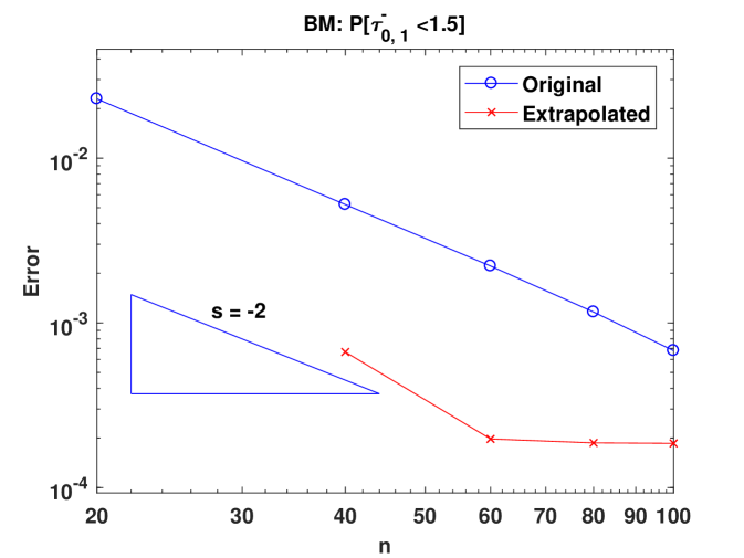
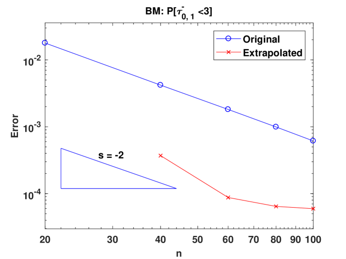
Figure 1 shows the convergence of [τL,Dt]\mathbb{P}[\tau_{L,D}^{-}\leq t] under the standard BM model by plotting errors against the number of CTMC states. Apparently we can observe second order convergence in both plots (see the blue lines) for t=1.5t=1.5 and t=3.0t=3.0, which verifies the theoretical convergence rate. Furthermore, the plots demonstrate that Richardson’s extrapolation can substantially reduce the error as seen from the red lines.

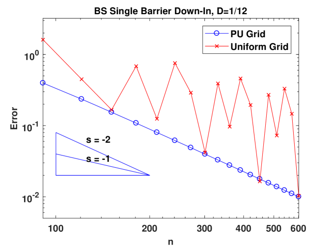
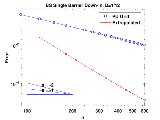
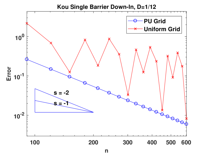
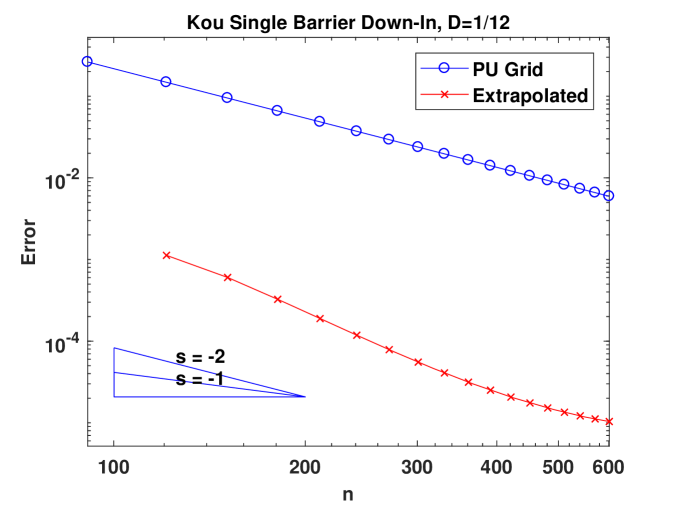
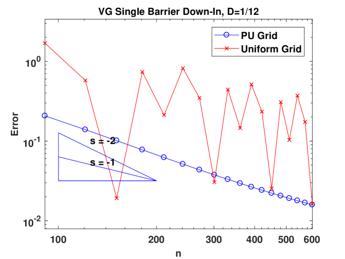
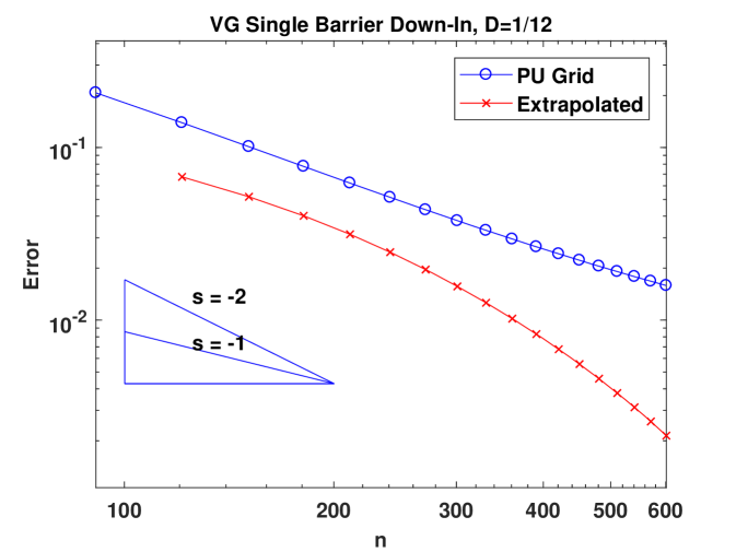
Figure 2 presents the convergence behavior of CTMC approximation for a sing-barrier down-and-in Parisian option under the BS model, Kou’s model and the VG model, respectively. In the left panel, we compare two different grids: a picewise uniform grid with LL on the grid and KK placed midway between two adjacent grid points (see (4.80)) and a uniform grid. For all three models, when the uniform grid is used, convergence is only first order. Moreover, there are big oscillations and this means Richardson’s extrapolation cannot be applied. In contrast, using the grid we design, convergence becomes second order and smooth in all the models. The results for the BS model justify our theoretical results. Although we don’t have proof for models with jumps, these numerical examples suggest that our grid design would also work for jump models. The plots in the right panel showcase the effectiveness of Richardson’s extrapolation. We also provide the numerical values for the original and extrapolated results in Table 1, 2 and 3. In Section A.4, we extend our algorithm to deal with regime-switching models. As an example, we consider the regime-switching BS model and the good performance of our method can be seen from the results in Table 4.

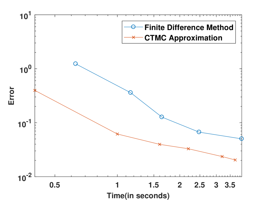
We compare our method with the explicit finite difference scheme developed in Wilmott (2013). The results are shown in Figure 3, which shows that our algorithm takes much less time (about 25% of the finite difference method) to achieve the same error level. The relatively slow performance of the finite difference approach should be expected as the PDE satisfied by the Parisian down-in option involves an additional dimension that records the length of excursion below the barrier and time discretization is required.

Refer to caption
Refer to caption
Figure 1: The convergence of [τL,Dt]\mathbb{P}[\tau_{L,D}^{-}\leq t] of a standard Brownian motion with L=0,D=1L=0,D=1 and t=1.5,3t=1.5,3. The benchmark for calculating the error is given by the solution in Dassios and Lim (2013).
Refer to caption
Refer to caption
Refer to caption
Refer to caption
Refer to caption
Refer to caption
Figure 2: Convergence of CTMC approximation for a single-barrier down-and-in Parisian option under the BS model, Kou’s model and the VG model. The benchmarks are obtained from CTMC approximation with very fine grids, and they match values from Monte Carlo simulation with a large number of replications.
Refer to caption
Figure 3: A comparison of CTMC approximation with finite difference method.
nn Exact CTMC Error Rel. Err. Time/s Extra. Error Rel. Err.
91 1.97866 1.58183 3.97E-01 20.06% 0.1
121 1.97866 1.74318 2.35E-01 11.90% 0.2 1.95326 2.54E-02 1.28%
151 1.97866 1.82432 1.54E-01 7.80% 0.2 1.96990 8.76E-03 0.44%
181 1.97866 1.87017 1.08E-01 5.48% 0.3 1.97513 3.53E-03 0.18%
211 1.97866 1.89839 8.03E-02 4.06% 0.3 1.97701 1.65E-03 0.08%
Table 1: Errors for the original and extrapolated results for the down-and-in Parisian option under the BS model.
nn Exact CTMC Error Rel. Err. Time/s Extra. Error Rel. Err.
91 4.55552 4.29302 2.63E-01 5.76% 0.4
121 4.55552 4.40754 1.48E-01 3.25% 0.5 4.55665 1.13E-03 0.02%
151 4.55552 4.46071 9.48E-02 2.08% 0.6 4.55611 5.90E-04 0.01%
181 4.55552 4.48963 6.59E-02 1.45% 0.8 4.55584 3.15E-04 0.01%
211 4.55552 4.50709 4.84E-02 1.06% 1.1 4.55573 2.10E-04 0.00%
Table 2: Errors for the original and extrapolated results for the down-and-in Parisian option under Kou’s model.
nn Exact CTMC Error Rel. Err. Time/s Extra. Error Rel. Err.
391 1.05872 1.03818 2.05E-02 1.94% 11.5
421 1.05872 1.03961 1.91E-02 1.81% 13.8 1.05825 4.72E-04 0.04%
451 1.05872 1.04084 1.79E-02 1.69% 15.9 1.05810 6.19E-04 0.06%
481 1.05872 1.04192 1.68E-02 1.59% 17.3 1.05816 5.64E-04 0.05%
511 1.05872 1.04286 1.59E-02 1.50% 19.6 1.05793 7.89E-04 0.07%
Table 3: Errors for the original and extrapolated results for the down-and-in Parisian option under the VG model.
nn Exact CTMC Error Rel. Err. Time/s Extra. Error Rel. Err.
91 4.30229 3.98449 3.18E-01 7.39% 2.0
121 4.30229 4.12057 1.82E-01 4.22% 3.4 4.29775 4.54E-03 0.11%
151 4.30229 4.18514 1.17E-01 2.72% 6.5 4.30099 1.30E-03 0.03%
181 4.30229 4.22062 8.17E-02 1.90% 9.9 4.30184 4.51E-04 0.01%
211 4.30229 4.24215 6.01E-02 1.40% 13.8 4.30213 1.66E-04 0.00%
Table 4: Errors for the original and extrapolated results for the down-and-in Parisian option under the regime-switching BS model. The benchmark is obtained from CTMC approximation with very fine grids, and it matches the result of Monte Carlo simulation with a large number of replications.

6 Conclusions

Our approach based on CTMC approximation is an efficient, accurate and flexible way to deal with Parisian stopping times and the related option pricing problems. It is applicable to general one-dimensional Markovian models and its convergence can be proved in a general setting. Moreover, extensions to regime-switching and stochastic volatility models as well as more complicated problems involving Parisian stopping times can be readily developed. We are also able to derive sharp estimate of the convergence rate for diffusion models. In general, convergence of CTMC approximation is first order, but we can improve it to second order with a proper grid design which places the Parisian barrier on the grid and all the discontinuities of the payoff function midway between two adjacent grid points. Such a grid can be easily constructed using a piecewise uniform structure. Our grid design also attains second order convergence in jump models as shown by the numerical examples. Furthermore, it ensures smooth convergence for both diffusion and jump models, which enables us to apply Richardson’s extrapolation to achieve significant reduction in the error. In future research, it would be interesting to develop effective hedging strategies for Parisian options based on our method.

Acknowledgements

The research of Lingfei Li was supported by Hong Kong Research Grant Council General Research Fund Grant 14202117. The research of Gongqiu Zhang was supported by National Natural Science Foundation of China Grant 11801423 and Shenzhen Basic Research Program Project JCYJ20190813165407555.

Appendix A Several Extensions

In this section, we generalize our method for some more complicated situations to demonstrate the versality of our approach.

A.1 Multi-Sided Parisian Options

Define a Parisian stopping time for an arbitrary set as

τAD=inf{t0:1{YtA}(tgA,t)D},gA,t=sup{st:YsA}.\displaystyle\tau_{A}^{D}=\inf\{t\geq 0:1_{\{Y_{t}\in A\}}(t-g_{A,t})\geq D\},\ g_{A,t}=\sup\{s\leq t:Y_{s}\notin A\}. (A.1)

If A=(,L)A=(-\infty,L), then τAD=τL,D\tau_{A}^{D}=\tau_{L,D}^{-} and if A=(U,)A=(U,\infty), τAD=τU,D+\tau_{A}^{D}=\tau_{U,D}^{+}. The multi-sided Parisian stopping time can be defined as

τ𝒜D=min{τAD:A𝒜},\displaystyle\tau_{\mathcal{A}}^{D}=\min\{\tau_{A}^{D}:A\in\mathcal{A}\}, (A.2)

where 𝒜\mathcal{A} is a collection of subsets of \mathbb{R}. The double-barrier case corresponds to 𝒜={(,L),(U,)}\mathcal{A}=\{(-\infty,L),(U,\infty)\} with L<UL<U. We also let

TA=inf{t0:YtA},TA+=inf{t0:YtA}.\displaystyle T^{-}_{A}=\inf\{t\geq 0:Y_{t}\notin A\},\ T^{+}_{A}=\inf\{t\geq 0:Y_{t}\in A\}. (A.3)

Consider a finite state CTMC YY. For any x,yx,y in its state space 𝕊\mathbb{S}, let h(q,x;y)=𝔼x[eqτ𝒜D1{Yτ𝒜D=y}]h(q,x;y)=\mathbb{E}_{x}\left[e^{-q\tau_{\mathcal{A}}^{D}}1_{\{Y_{\tau_{\mathcal{A}}^{D}}=y\}}\right]. Define B=A𝒜AB=\cup_{A\in\mathcal{A}}A. Then, by the conditioning argument, we obtain

h(q,x;y)\displaystyle h(q,x;y) =A𝒜eqD𝔼x[1{TAD,YD=y}]×1{xA}\displaystyle=\sum_{A\in\mathcal{A}}e^{-qD}\mathbb{E}_{x}\left[1_{\{T_{A}^{-}\geq D,Y_{D}=y\}}\right]\times 1_{\{x\in A\}} (A.4)
+A𝒜zA𝔼x[eqTA1{TA<D,YTA=z}]h(q,z;y)×1{xA}\displaystyle\quad+\sum_{A\in\mathcal{A}}\sum_{z\notin A}\mathbb{E}_{x}\left[e^{-qT_{A}^{-}}1_{\{T_{A}^{-}<D,Y_{T_{A}^{-}}=z\}}\right]h(q,z;y)\times 1_{\{x\in A\}} (A.5)
+zB𝔼x[eqTB+1{YTB+=z}]h(q,z;y)×1{xB}.\displaystyle\quad+\sum_{z\in B}\mathbb{E}_{x}\left[e^{-qT_{B}^{+}}1_{\{Y_{T_{B}^{+}}=z\}}\right]h(q,z;y)\times 1_{\{x\notin B\}}. (A.6)

Let vA(D,x;y)=𝔼x[1{TAD,YD=y}]v_{A}(D,x;y)=\mathbb{E}_{x}\left[1_{\{T_{A}^{-}\geq D,Y_{D}=y\}}\right]. It solves

{vAD(D,x;y)=𝑮vA(D,x;y),xA,D>0vA(D,x;y)=0,xA,D>0,vA(0,x;y)=1{x=y}.\displaystyle\begin{cases}\frac{\partial v_{A}}{\partial D}(D,x;y)={\boldsymbol{G}}v_{A}(D,x;y),\ x\in A,D>0\\ v_{A}(D,x;y)=0,\ x\notin A,D>0,\\ v_{A}(0,x;y)=1_{\{x=y\}}.\end{cases} (A.7)

Let uA(q,D,x;z)=𝔼x[eqTA1{TA<D,YTA=z}]u^{-}_{A}(q,D,x;z)=\mathbb{E}_{x}\left[e^{-qT_{A}^{-}}1_{\{T_{A}^{-}<D,Y_{T_{A}^{-}}=z\}}\right], then it satisfies,

{uAD(q,D,x;z)=𝑮uA(q,D,x;z)quA(q,D,x;z),xA,D>0,uA(q,D,x;z)=1{x=z},xA,D>0,uA(q,0,x;z)=0.\displaystyle\begin{cases}\frac{\partial u^{-}_{A}}{\partial D}(q,D,x;z)={\boldsymbol{G}}u^{-}_{A}(q,D,x;z)-qu^{-}_{A}(q,D,x;z),\ x\in A,D>0,\\ u^{-}_{A}(q,D,x;z)=1_{\{x=z\}},\ x\notin A,D>0,\\ u^{-}_{A}(q,0,x;z)=0.\end{cases} (A.8)

We can rewrite it as uA(q,D,x;z)=u1,A(q,x;z)u2,A(q,D,x;z)u^{-}_{A}(q,D,x;z)=u^{-}_{1,A}(q,x;z)-u^{-}_{2,A}(q,D,x;z), and these two parts satisfy

{𝑮u1,A(q,x;z)qu1,A(q,x;z)=0,xA,u1,A(q,x;z)=1{x=z},xA,\displaystyle\begin{cases}{\boldsymbol{G}}u^{-}_{1,A}(q,x;z)-qu^{-}_{1,A}(q,x;z)=0,\ x\in A,\\ u^{-}_{1,A}(q,x;z)=1_{\{x=z\}},\ x\notin A,\end{cases} (A.9)

and

{u2,AD(q,D,x;z)=𝑮u2,A(q,D,x;z)qu2,A(q,D,x;z),xA,u2,A(q,D,x;z)=0,xA,D>0,u2,A(q,0,x;z)=u1,A(q,x;z).\displaystyle\begin{cases}\frac{\partial u^{-}_{2,A}}{\partial{D}}(q,D,x;z)={\boldsymbol{G}}u^{-}_{2,A}(q,D,x;z)-qu^{-}_{2,A}(q,D,x;z),\ x\in A,\\ u^{-}_{2,A}(q,D,x;z)=0,\ x\notin A,D>0,\\ u^{-}_{2,A}(q,0,x;z)=u^{-}_{1,A}(q,x;z).\end{cases} (A.10)

Let u+(q,x;z)=𝔼x[eqTB+1{YTB+=z}]u^{+}(q,x;z)=\mathbb{E}_{x}\left[e^{-qT_{B}^{+}}1_{\{Y_{T_{B}^{+}}=z\}}\right]. It is the solution to

{𝑮u+(q,x;z)qu+(q,x;z)=0,xB,u+(q,x;z)=1{x=z},xB.\displaystyle\begin{cases}{\boldsymbol{G}}u^{+}(q,x;z)-qu^{+}(q,x;z)=0,\ x\notin B,\\ u^{+}(q,x;z)=1_{\{x=z\}},\ x\in B.\end{cases} (A.11)

Let 𝑰A=diag((1{xA})x𝕊){\boldsymbol{I}}_{A}=\operatorname{diag}((1_{\{x\in A\}})_{x\in\mathbb{S}}). The solutions to the above equations are given as follows:

𝑽A=(vA(D,x;y))x,y𝕊=exp(𝑰A𝑮D)𝑰A,\displaystyle{\boldsymbol{V}}_{A}=\left(v_{A}(D,x;y)\right)_{x,y\in\mathbb{S}}=\exp\left({\boldsymbol{I}}_{A}{\boldsymbol{G}}D\right){\boldsymbol{I}}_{A}, (A.12)
𝑼1,A(q)=(u1,A(q,x;z))x,z𝕊=(𝑰𝑰A𝑰A(𝑮q𝑰))1(𝑰𝑰A),\displaystyle{\boldsymbol{U}}_{1,A}^{-}(q)=\left(u^{-}_{1,A}(q,x;z)\right)_{x,z\in\mathbb{S}}=\left({\boldsymbol{I}}-{\boldsymbol{I}}_{A}-{\boldsymbol{I}}_{A}({\boldsymbol{G}}-q{\boldsymbol{I}})\right)^{-1}({\boldsymbol{I}}-{\boldsymbol{I}}_{A}), (A.13)
𝑼2,A(q)=(u2,A(q,D,x;z))x,z𝕊=exp(𝑰A𝑮D)𝑰A𝑼1,A(q),\displaystyle{\boldsymbol{U}}_{2,A}^{-}(q)=\left(u^{-}_{2,A}(q,D,x;z)\right)_{x,z\in\mathbb{S}}=\exp\left({\boldsymbol{I}}_{A}{\boldsymbol{G}}D\right){\boldsymbol{I}}_{A}{\boldsymbol{U}}_{1,A}^{-}(q), (A.14)
𝑼A(q)=(uA(q,D,x;z))x,z𝕊=𝑼1,A(q)𝑼2,A(q),\displaystyle{\boldsymbol{U}}^{-}_{A}(q)=\left(u^{-}_{A}(q,D,x;z)\right)_{x,z\in\mathbb{S}}={\boldsymbol{U}}_{1,A}^{-}(q)-{\boldsymbol{U}}_{2,A}^{-}(q), (A.15)
𝑼+(q)=(u+(q,x;z))x,z𝕊=(𝑰B(𝑰𝑰B)(𝑮q𝑰))1𝑰B.\displaystyle{\boldsymbol{U}}^{+}(q)=\left(u^{+}(q,x;z)\right)_{x,z\in\mathbb{S}}=\left({\boldsymbol{I}}_{B}-({\boldsymbol{I}}-{\boldsymbol{I}}_{B})({\boldsymbol{G}}-q{\boldsymbol{I}})\right)^{-1}{\boldsymbol{I}}_{B}. (A.16)

Then, we obtain

𝑯(q)=(h(q,x;y))x,y𝕊=eqD(𝑰A𝒜𝑰A𝑼A(q)(𝑰𝑰B)𝑼+(q))1A𝒜𝑰A𝑽A.\displaystyle{\boldsymbol{H}}(q)=\left(h(q,x;y)\right)_{x,y\in\mathbb{S}}=e^{-qD}\left({\boldsymbol{I}}-\sum_{A\in\mathcal{A}}{\boldsymbol{I}}_{A}{\boldsymbol{U}}^{-}_{A}(q)-({\boldsymbol{I}}-{\boldsymbol{I}}_{B}){\boldsymbol{U}}^{+}(q)\right)^{-1}\sum_{A\in\mathcal{A}}{\boldsymbol{I}}_{A}{\boldsymbol{V}}_{A}. (A.17)

Now consider a multi-sided Parisian option with price u(t,x)=𝔼x[1{τ𝒜Dt}f(Yt)]u(t,x)=\mathbb{E}_{x}\left[1_{\{\tau_{\mathcal{A}}^{D}\leq t\}}f(Y_{t})\right]. Using the arguments in the single-sided case, we can derive that the Laplace transform u~(q,x)=0eqtu(t,x)𝑑t\tilde{u}(q,x)=\int_{0}^{\infty}e^{-qt}u(t,x)dt is given by

𝒖~(q)=(u~(q,x))x𝕊=𝑯(q)(q𝑰𝑮)1𝒇.\displaystyle\widetilde{\boldsymbol{u}}(q)=\left(\tilde{u}(q,x)\right)_{x\in\mathbb{S}}={\boldsymbol{H}}(q)(q{\boldsymbol{I}}-{\boldsymbol{G}})^{-1}{\boldsymbol{f}}. (A.18)

A.2 Mixed Barrier and Parisian Options

CTMC approximation can also be generalized to derive the joint distribution of Parisian stopping times and first passage times. For example, Dassios and Zhang (2016) introduce the so-called MinParisianHit option which is triggered either when the age of an excursion above LL reaches time DD or a barrier B>LB>L is crossed by the underlying asset price process StS_{t}. The MinParisianHit option price can be approximated as

minPHCiu(t,x;L,D,B)=erft𝔼x[1{τL,D+τB+t}f(Yt)].\displaystyle\text{minPHC}_{i}^{u}(t,x;L,D,B)=e^{-r_{f}t}\mathbb{E}_{x}\left[1_{\{\tau_{L,D}^{+}\wedge\tau_{B}^{+}\leq t\}}f(Y_{t})\right]. (A.19)

where YtY_{t} is a CTMC with state space 𝕊\mathbb{S} and transition rate matrix 𝑮{\boldsymbol{G}} to approximate the underlying price process. To price the option, it suffices to substitute τL,D\tau_{L,D}^{-} by τL,D+τB+\tau_{L,D}^{+}\wedge\tau_{B}^{+} in the proof of Theorem 2.2 and find the Laplace transform of τL,D+τB+\tau_{L,D}^{+}\wedge\tau_{B}^{+} under the model YtY_{t}. Let h1(q,x;y)=𝔼x[eqτL,D+τB+1{τL,D+τB+=y}]h_{1}(q,x;y)=\mathbb{E}_{x}[e^{-q\tau_{L,D}^{+}\wedge\tau_{B}^{+}}1_{\{\tau_{L,D}^{+}\wedge\tau_{B}^{+}=y\}}]. Using the conditioning argument, we can show that h1(q,x,y)h_{1}(q,x,y) satisfies a linear system

h1(q,x;y)\displaystyle h_{1}(q,x;y) =1{xB,x=y}+1{xL}z>L𝔼x[eqτ¯L+1{Yτ¯L+=z}]h1(q,z;y)\displaystyle=1_{\{x\geq B,x=y\}}+1_{\{x\leq L\}}\sum_{z>L}\mathbb{E}_{x}\left[e^{-q\overline{\tau}_{L}^{+}}1_{\{Y_{\overline{\tau}_{L}^{+}}=z\}}\right]h_{1}(q,z;y) (A.20)
+1{L<x<B}𝔼x[eqτB+1{τB+<D,YτB+=y}]\displaystyle\quad+1_{\{L<x<B\}}\mathbb{E}_{x}\left[e^{-q\tau_{B}^{+}}1_{\{\tau_{B}^{+}<D,Y_{\tau_{B}^{+}}=y\}}\right] (A.21)
+1{L<x<B}zL𝔼x[eqτ¯L1{τ¯L<DτB+,Yτ¯L=z}]h1(q,z;y)\displaystyle\quad+1_{\{L<x<B\}}\sum_{z\leq L}\mathbb{E}_{x}\left[e^{-q\overline{\tau}_{L}^{-}}1_{\{\overline{\tau}_{L}^{-}<D\leq\tau_{B}^{+},Y_{\overline{\tau}_{L}^{-}}=z\}}\right]h_{1}(q,z;y) (A.22)
+1{L<x<B}eqD𝔼x[1{τ¯LτB+D,YD=y}],\displaystyle\quad+1_{\{L<x<B\}}e^{-qD}\mathbb{E}_{x}\left[1_{\{\overline{\tau}_{L}^{-}\wedge\tau_{B}^{+}\geq D,Y_{D}=y\}}\right], (A.23)

where τ¯L+=inf{t0:Yt>L}\overline{\tau}_{L}^{+}=\inf\{t\geq 0:Y_{t}>L\} and τ¯L=inf{t0:YtL}\overline{\tau}_{L}^{-}=\inf\{t\geq 0:Y_{t}\leq L\} (they are slightly different from τL+\tau_{L}^{+} and τL\tau_{L}^{-} defined in Section 2).

We next analyze each term. For (A.20), let u¯(q,x;z)=𝔼x[eqτ¯L+1{Yτ¯L+=z}]\overline{u}(q,x;z)=\mathbb{E}_{x}\left[e^{-q\overline{\tau}_{L}^{+}}1_{\{Y_{\overline{\tau}_{L}^{+}}=z\}}\right]. It satisfies

{𝑮u¯(q,x;z)qu¯(q,x;z)=0,x(,L]𝕊,u¯(q,x;z)=1{x=z},x(L,)𝕊,\displaystyle\begin{cases}{\boldsymbol{G}}\overline{u}(q,x;z)-q\overline{u}(q,x;z)=0,\ x\in(-\infty,L]\cap\mathbb{S},\\ \overline{u}(q,x;z)=1_{\{x=z\}},\ x\in(L,\infty)\cap\mathbb{S},\\ \end{cases} (A.24)

For (A.21), let v(q,D,x;y)=𝔼x[eqτB+1{τB+<D,YτB+=y}]v(q,D,x;y)=\mathbb{E}_{x}\left[e^{-q\tau_{B}^{+}}1_{\{\tau_{B}^{+}<D,Y_{\tau_{B}^{+}}=y\}}\right]. It is the solution to

{vD(q,D,x;y)=𝑮v(q,D,x;y)qv(q,D,x;y),D>0,x(,B)𝕊,v(q,D,x;y)=1{x=y},D>0,x[B,)𝕊,v(q,0,x;y)=0,x𝕊.\displaystyle\begin{cases}\frac{\partial v}{\partial D}(q,D,x;y)={\boldsymbol{G}}v(q,D,x;y)-qv(q,D,x;y),\ D>0,\ x\in(-\infty,B)\cap\mathbb{S},\\ v(q,D,x;y)=1_{\{x=y\}},\ D>0,\ x\in[B,\infty)\cap\mathbb{S},\\ v(q,0,x;y)=0,\ x\in\mathbb{S}.\end{cases} (A.25)

v(q,D,x;y)v(q,D,x;y) can be split as v1(q,x;y)v2(q,D,x;y)v_{1}(q,x;y)-v_{2}(q,D,x;y) with v1(q,x;y)v_{1}(q,x;y) satisfying

{𝑮v1(q,x;y)qv1(q,x;y)=0,x(,B)𝕊,v1(q,x;y)=1{x=y},x[B,)𝕊,\displaystyle\begin{cases}{\boldsymbol{G}}v_{1}(q,x;y)-qv_{1}(q,x;y)=0,\ x\in(-\infty,B)\cap\mathbb{S},\\ v_{1}(q,x;y)=1_{\{x=y\}},\ x\in[B,\infty)\cap\mathbb{S},\\ \end{cases} (A.26)

and v2(q,D,x;y)v_{2}(q,D,x;y) satisfying

{v2D(q,D,x;y)=𝑮v2(q,D,x;y)qv2(q,D,x;y),D>0,x(,B)𝕊,v2(q,D,x;y)=0,D>0,x[B,)𝕊,v2(q,0,x;y)=v1(q,x;y),x𝕊.\displaystyle\begin{cases}\frac{\partial v_{2}}{\partial D}(q,D,x;y)={\boldsymbol{G}}v_{2}(q,D,x;y)-qv_{2}(q,D,x;y),\ D>0,\ x\in(-\infty,B)\cap\mathbb{S},\\ v_{2}(q,D,x;y)=0,\ D>0,\ x\in[B,\infty)\cap\mathbb{S},\\ v_{2}(q,0,x;y)=v_{1}(q,x;y),\ x\in\mathbb{S}.\end{cases} (A.27)

For (A.22), let u(q,D,x;z)=𝔼x[eqτ¯L1{τ¯L<DτB+,Yτ¯L=z}]u(q,D,x;z)=\mathbb{E}_{x}\left[e^{-q\overline{\tau}_{L}^{-}}1_{\{\overline{\tau}_{L}^{-}<D\leq\tau_{B}^{+},Y_{\overline{\tau}_{L}^{-}}=z\}}\right]. It solves

{uD(q,D,x;z)=𝑮u(q,D,x;z)qu(q,D,x;z),D>0,x(L,B)𝕊,u(q,D,x;z)=1{x=z}𝔼x[1{τB+D}],D>0,x(,L]𝕊,u(q,D,x;z)=0,D>0,x[B,)𝕊,u(q,0,x;z)=0,x𝕊.\displaystyle\begin{cases}\frac{\partial u}{\partial D}(q,D,x;z)={\boldsymbol{G}}u(q,D,x;z)-qu(q,D,x;z),\ D>0,\ x\in(L,B)\cap\mathbb{S},\\ u(q,D,x;z)=1_{\{x=z\}}\mathbb{E}_{x}\left[1_{\{\tau_{B}^{+}\geq D\}}\right],\ D>0,\ x\in(-\infty,L]\cap\mathbb{S},\\ u(q,D,x;z)=0,\ D>0,\ x\in[B,\infty)\cap\mathbb{S},\\ u(q,0,x;z)=0,\ x\in\mathbb{S}.\end{cases} (A.28)

u(q,D,x;z)u(q,D,x;z) can be expressed as u1(q,x;z)u2(q,D,x;z)u_{1}(q,x;z)-u_{2}(q,D,x;z) with u1(q,x;z)u_{1}(q,x;z) satisfying

{𝑮u1(q,x;z)qu1(q,x;z)=0,x(L,B)𝕊,u1(q,x;z)=1{x=z}𝔼x[1{τB+D}],x(,L]𝕊,u1(q,x;z)=0,x[B,)𝕊,\displaystyle\begin{cases}{\boldsymbol{G}}u_{1}(q,x;z)-qu_{1}(q,x;z)=0,\ x\in(L,B)\cap\mathbb{S},\\ u_{1}(q,x;z)=1_{\{x=z\}}\mathbb{E}_{x}\left[1_{\{\tau_{B}^{+}\geq D\}}\right],\ x\in(-\infty,L]\cap\mathbb{S},\\ u_{1}(q,x;z)=0,\ \ x\in[B,\infty)\cap\mathbb{S},\end{cases} (A.29)

and u2(q,D,x;z)u_{2}(q,D,x;z) satisfying

{u2D(q,D,x;z)=𝑮u2(q,D,x;z)qu2(q,D,x;z),D>0,x(L,B)𝕊,u2(q,D,x;z)=0,D>0,x(,L]𝕊,u2(q,D,x;z)=0,D>0,x[B,)𝕊,u2(q,0,x;z)=u1(q,x;z),x𝕊.\displaystyle\begin{cases}\frac{\partial u_{2}}{\partial D}(q,D,x;z)={\boldsymbol{G}}u_{2}(q,D,x;z)-qu_{2}(q,D,x;z),\ D>0,\ x\in(L,B)\cap\mathbb{S},\\ u_{2}(q,D,x;z)=0,\ D>0,\ x\in(-\infty,L]\cap\mathbb{S},\\ u_{2}(q,D,x;z)=0,\ D>0,\ x\in[B,\infty)\cap\mathbb{S},\\ u_{2}(q,0,x;z)=u_{1}(q,x;z),\ x\in\mathbb{S}.\end{cases} (A.30)

For (A.23), let w(D,x;y)=𝔼x[1{τ¯LτB+D,YD=y}]w(D,x;y)=\mathbb{E}_{x}\left[1_{\{\overline{\tau}_{L}^{-}\wedge\tau_{B}^{+}\geq D,Y_{D}=y\}}\right]. It solves

{wD(D,x;y)=𝑮w(D,x;y),D>0,x(L,B)𝕊,w(D,x;y)=0,D>0,x𝕊\(L,B),w(0,x;y)=1{x=y},x𝕊.\displaystyle\begin{cases}\frac{\partial w}{\partial D}(D,x;y)={\boldsymbol{G}}w(D,x;y),\ D>0,\ x\in(L,B)\cap\mathbb{S},\\ w(D,x;y)=0,\ D>0,\ x\in\mathbb{S}\backslash(L,B),\\ w(0,x;y)=1_{\{x=y\}},\ x\in\mathbb{S}.\end{cases} (A.31)

Let 𝑰¯L+=diag((1{x>L})x𝕊)\overline{\boldsymbol{I}}_{L}^{+}=\operatorname{diag}\left((1_{\{x>L\}})_{x\in\mathbb{S}}\right), 𝑰¯L=diag((1{xL})x𝕊)\overline{\boldsymbol{I}}_{L}^{-}=\operatorname{diag}\left((1_{\{x\leq L\}})_{x\in\mathbb{S}}\right), 𝑰L,B=𝑰¯L+𝑰B{\boldsymbol{I}}_{L,B}=\overline{\boldsymbol{I}}_{L}^{+}{\boldsymbol{I}}_{B}^{-} (they are slightly different from 𝑰L+{\boldsymbol{I}}_{L}^{+} and 𝑰L{\boldsymbol{I}}_{L}^{-} defined in Section 2). The solutions to the above equations are given by

𝑼¯(q)=(u¯(q,x;z))x,z𝕊=(q𝑰¯L𝑰¯L𝑮+𝑰¯L+)1𝑰¯L+,\displaystyle\overline{\boldsymbol{U}}(q)=\left(\overline{u}(q,x;z)\right)_{x,z\in\mathbb{S}}=\left(q\overline{\boldsymbol{I}}_{L}^{-}-\overline{\boldsymbol{I}}_{L}^{-}{\boldsymbol{G}}+\overline{\boldsymbol{I}}_{L}^{+}\right)^{-1}\overline{\boldsymbol{I}}_{L}^{+}, (A.32)
𝑽1(q)=(v1(q,x;y))x,y𝕊=(q𝑰B𝑰B𝑮+𝑰B+)1𝑰B+,\displaystyle{\boldsymbol{V}}_{1}(q)=\left(v_{1}(q,x;y)\right)_{x,y\in\mathbb{S}}=\left(q{\boldsymbol{I}}_{B}^{-}-{\boldsymbol{I}}_{B}^{-}{\boldsymbol{G}}+{\boldsymbol{I}}_{B}^{+}\right)^{-1}{\boldsymbol{I}}_{B}^{+}, (A.33)
𝑽2(q)=(v2(q,D,x;y))x,y𝕊=exp(𝑰B𝑮q𝑰B)𝑰B𝑽1(q),\displaystyle{\boldsymbol{V}}_{2}(q)=\left(v_{2}(q,D,x;y)\right)_{x,y\in\mathbb{S}}=\exp\left({\boldsymbol{I}}_{B}^{-}{\boldsymbol{G}}-q{\boldsymbol{I}}_{B}^{-}\right){\boldsymbol{I}}_{B}^{-}{\boldsymbol{V}}_{1}(q), (A.34)
𝑼1(q)=(u1(q,x;z))x,z𝕊=(q𝑰L,B𝑰L,B𝑮+𝑰𝑰L,B)1𝑰¯Ldiag(exp(𝑰B𝑮D)𝒆B),\displaystyle{\boldsymbol{U}}_{1}(q)=\left(u_{1}(q,x;z)\right)_{x,z\in\mathbb{S}}=\left(q{\boldsymbol{I}}_{L,B}-{\boldsymbol{I}}_{L,B}{\boldsymbol{G}}+{\boldsymbol{I}}-{\boldsymbol{I}}_{L,B}\right)^{-1}\overline{\boldsymbol{I}}_{L}^{-}\operatorname{diag}\left(\exp\left({\boldsymbol{I}}_{B}^{-}{\boldsymbol{G}}D\right){\boldsymbol{e}}_{B}^{-}\right), (A.35)
𝑼2(q)=(u2(q,D,x;z))x,z𝕊=exp(𝑰L,B𝑮q𝑰L,B)𝑰L,B𝑼1(q),\displaystyle{\boldsymbol{U}}_{2}(q)=\left(u_{2}(q,D,x;z)\right)_{x,z\in\mathbb{S}}=\exp\left({\boldsymbol{I}}_{L,B}{\boldsymbol{G}}-q{\boldsymbol{I}}_{L,B}\right){\boldsymbol{I}}_{L,B}{\boldsymbol{U}}_{1}(q), (A.36)
𝑾=(w(D,x;y))x,y𝕊=exp(𝑰L,B𝑮D)𝑰L,B,\displaystyle{\boldsymbol{W}}=\left(w(D,x;y)\right)_{x,y\in\mathbb{S}}=\exp\left({\boldsymbol{I}}_{L,B}{\boldsymbol{G}}D\right){\boldsymbol{I}}_{L,B}, (A.37)

where 𝒆B=(1{x<B})x𝕊{\boldsymbol{e}}_{B}^{-}=(1_{\{x<B\}})_{x\in\mathbb{S}}. Let 𝑯1(q)=(h1(q,x;y))x,y𝕊{\boldsymbol{H}}_{1}(q)=\left(h_{1}(q,x;y)\right)_{x,y\in\mathbb{S}}, which satisfies

𝑯1(q)=𝑰B++𝑰L,B(𝑽1(q)𝑽2(q))+𝑰L,B(𝑼1(q)𝑼2(q))𝑯1(q)+𝑰¯L𝑼¯(q)𝑯1(q)+eqD𝑰L,B𝑾.\displaystyle{\boldsymbol{H}}_{1}(q)={\boldsymbol{I}}_{B}^{+}+{\boldsymbol{I}}_{L,B}\left({\boldsymbol{V}}_{1}(q)-{\boldsymbol{V}}_{2}(q)\right)+{\boldsymbol{I}}_{L,B}\left({\boldsymbol{U}}_{1}(q)-{\boldsymbol{U}}_{2}(q)\right){\boldsymbol{H}}_{1}(q)+\overline{\boldsymbol{I}}_{L}^{-}\overline{\boldsymbol{U}}(q){\boldsymbol{H}}_{1}(q)+e^{-qD}{\boldsymbol{I}}_{L,B}{\boldsymbol{W}}. (A.38)

The solution is

𝑯1(q)=(𝑰𝑼(q))1𝑽(q),\displaystyle{\boldsymbol{H}}_{1}(q)=\left({\boldsymbol{I}}-{\boldsymbol{U}}(q)\right)^{-1}{\boldsymbol{V}}(q), (A.39)

where 𝑼(q)=𝑰L,B(𝑼1(q)𝑼2(q))+𝑰¯L𝑼¯(q){\boldsymbol{U}}(q)={\boldsymbol{I}}_{L,B}\left({\boldsymbol{U}}_{1}(q)-{\boldsymbol{U}}_{2}(q)\right)+\overline{\boldsymbol{I}}_{L}^{-}\overline{\boldsymbol{U}}(q) and 𝑽(q)=𝑰B++𝑰L,B(𝑽1(q)𝑽2(q))+eqD𝑰L,B𝑾{\boldsymbol{V}}(q)={\boldsymbol{I}}_{B}^{+}+{\boldsymbol{I}}_{L,B}\left({\boldsymbol{V}}_{1}(q)-{\boldsymbol{V}}_{2}(q)\right)+e^{-qD}{\boldsymbol{I}}_{L,B}{\boldsymbol{W}}. Consider the Laplace transform

u~i(q,x)=0eqtminPHCiu(t,x;L,D,B)𝑑t,(q)>0.\displaystyle\widetilde{u}_{i}(q,x)=\int_{0}^{\infty}e^{-qt}\text{minPHC}_{i}^{u}(t,x;L,D,B)dt,\ \Re(q)>0. (A.40)

It can be obtained as

𝒖~i(q)=(u~i(q,x))x𝕊=𝑯1(q+rf)((q+rf)𝑰𝑮)1𝒇.\displaystyle\widetilde{\boldsymbol{u}}_{i}(q)=\left(\widetilde{u}_{i}(q,x)\right)_{x\in\mathbb{S}}={\boldsymbol{H}}_{1}(q+r_{f})\left((q+r_{f}){\boldsymbol{I}}-{\boldsymbol{G}}\right)^{-1}{\boldsymbol{f}}. (A.41)

A.3 Pricing Parisian Bonds

Recently, Dassios et al. (2020) propose a Parisian type of bonds, whose payoff depends on whether the excursion of the interest rate above some level LL exceeds a given duration before maturity, i.e., h(Rτ)1{τ<T}h(R_{\tau})1_{\{\tau<T\}}, where TT is the bond maturity, RR is the short rate process, h()h(\cdot) is the payoff function, and

τ=inf{t>0:Ut=D},Ut=tsup{s<t:RsL}.\displaystyle\tau=\inf\{t>0:U_{t}=D\},\ U_{t}=t-\sup\{s<t:R_{s}\leq L\}. (A.42)

Then its price can be written as,

P(T,x)=𝔼x[e0τRt𝑑tf(Rτ)1{τ<T}],\displaystyle P(T,x)=\mathbb{E}_{x}\left[e^{-\int_{0}^{\tau}R_{t}dt}f(R_{\tau})1_{\{\tau<T\}}\right], (A.43)

where 𝔼x[]=𝔼[|R0=x]\mathbb{E}_{x}[\cdot]=\mathbb{E}[\cdot|R_{0}=x]. We can calculate its Laplace transform w.r.t. TT as,

P~(q,x)=0eqTP(T,x)𝑑T=1q𝔼x[e0τ(q+Rt)𝑑tf(Rτ)].\displaystyle\widetilde{P}(q,x)=\int_{0}^{\infty}e^{-qT}P(T,x)dT=\frac{1}{q}\mathbb{E}_{x}\left[e^{-\int_{0}^{\tau}(q+R_{t})dt}f(R_{\tau})\right]. (A.44)

Suppose RR is a CTMC with state space 𝕊R\mathbb{S}_{R} to approximate the original short rate model (e.g., the CIR model considered in Dassios et al. (2020)). Let h(q,x)=𝔼x[e0τ(q+Rt)𝑑tf(Rτ)]h(q,x)=\mathbb{E}_{x}\left[e^{-\int_{0}^{\tau}(q+R_{t})dt}f(R_{\tau})\right] and τ¯L+\overline{\tau}_{L}^{+} and τ¯L\overline{\tau}_{L}^{-} are defined as in Section A.2. Then, using the conditioning argument, we obtain

h(q,x)\displaystyle h(q,x) =𝔼x[e0D(q+Rt)𝑑tf(RD)1{τ¯LD}]1{x>L}\displaystyle=\mathbb{E}_{x}\left[e^{-\int_{0}^{D}(q+R_{t})dt}f(R_{D})1_{\{\overline{\tau}_{L}^{-}\geq D\}}\right]1_{\{x>L\}} (A.45)
+zL𝔼x[e0τ¯L(q+Rt)𝑑t1{τ¯L<D,Rτ¯L=z}]1{x>L}h(q,z)\displaystyle\quad+\sum_{z\leq L}\mathbb{E}_{x}\left[e^{-\int_{0}^{\overline{\tau}_{L}^{-}}(q+R_{t})dt}1_{\{\overline{\tau}_{L}^{-}<D,R_{\overline{\tau}_{L}^{-}}=z\}}\right]1_{\{x>L\}}h(q,z) (A.46)
+z>L𝔼x[e0τ¯L+(q+Rt)𝑑t1{Rτ¯L+=z}]1{xL}h(q,z).\displaystyle\quad+\sum_{z>L}\mathbb{E}_{x}\left[e^{-\int_{0}^{\overline{\tau}_{L}^{+}}(q+R_{t})dt}1_{\{R_{\overline{\tau}_{L}^{+}}=z\}}\right]1_{\{x\leq L\}}h(q,z). (A.47)

Let 𝑮{\boldsymbol{G}} be the generator matrix of RR. Consider v(q,D,x)=𝔼x[e0D(q+Rt)𝑑tf(RD)1{τ¯LD}]v(q,D,x)=\mathbb{E}_{x}\left[e^{-\int_{0}^{D}(q+R_{t})dt}f(R_{D})1_{\{\overline{\tau}_{L}^{-}\geq D\}}\right]. It satisfies

{vD(q,D,x)=(𝑮𝑹q)v(q,D,x),D>0,x(L,)𝕊R,v(q,D,x)=0,D>0,x(,L]𝕊R,v(q,0,x)=f(x),x𝕊R,\displaystyle\begin{cases}\frac{\partial v}{\partial D}(q,D,x)=({\boldsymbol{G}}-{\boldsymbol{R}}_{q})v(q,D,x),\ D>0,x\in(L,\infty)\cap\mathbb{S}_{R},\\ v(q,D,x)=0,\ D>0,x\in(-\infty,L]\cap\mathbb{S}_{R},\\ v(q,0,x)=f(x),\ x\in\mathbb{S}_{R},\end{cases} (A.48)

where 𝑹q=diag((q+x)x𝕊R){\boldsymbol{R}}_{q}=\text{diag}\left((q+x)_{x\in\mathbb{S}_{R}}\right). Let u(q,D,x;z)=𝔼x[e0τ¯L(q+Rt)𝑑t1{τ¯L<D,Rτ¯L=z}]u^{-}(q,D,x;z)=\mathbb{E}_{x}\left[e^{-\int_{0}^{\overline{\tau}_{L}^{-}}(q+R_{t})dt}1_{\{\overline{\tau}_{L}^{-}<D,R_{\overline{\tau}_{L}^{-}}=z\}}\right]. It solves

{uD(q,D,x;z)=(𝑮𝑹q)u(q,D,x;z),D>0,x(L,)𝕊R,u(q,D,x;z)=1{x=z},D>0,x(,L]𝕊R,u(q,0,x;z)=0.\displaystyle\begin{cases}\frac{\partial u^{-}}{\partial D}(q,D,x;z)=({\boldsymbol{G}}-{\boldsymbol{R}}_{q})u^{-}(q,D,x;z),\ D>0,x\in(L,\infty)\cap\mathbb{S}_{R},\\ u^{-}(q,D,x;z)=1_{\{x=z\}},\ D>0,x\in(-\infty,L]\cap\mathbb{S}_{R},\\ u^{-}(q,0,x;z)=0.\end{cases} (A.49)

We can decomposed u(q,D,x;z)u^{-}(q,D,x;z) as u(q,D,x;z)=u1(q,x;z)u2(q,D,x;z)u^{-}(q,D,x;z)=u_{1}^{-}(q,x;z)-u_{2}^{-}(q,D,x;z) with them satisfying

{(𝑮𝑹q)u1(q,x;z)=0,x(L,)𝕊R,u1(q,x;z)=1{x=z},x(,L]𝕊R,\displaystyle\begin{cases}({\boldsymbol{G}}-{\boldsymbol{R}}_{q})u_{1}^{-}(q,x;z)=0,\ x\in(L,\infty)\cap\mathbb{S}_{R},\\ u_{1}^{-}(q,x;z)=1_{\{x=z\}},\ x\in(-\infty,L]\cap\mathbb{S}_{R},\end{cases} (A.50)

and

{u2D(q,D,x;z)=(𝑮𝑹q)u2(q,D,x;z),D>0,x(L,)𝕊R,u2(q,D,x;z)=0,D>0,x(,L]𝕊R,u2(q,0,x;z)=u1(q,x;z),x𝕊R.\displaystyle\begin{cases}\frac{\partial u_{2}^{-}}{\partial D}(q,D,x;z)=({\boldsymbol{G}}-{\boldsymbol{R}}_{q})u_{2}^{-}(q,D,x;z),\ D>0,x\in(L,\infty)\cap\mathbb{S}_{R},\\ u_{2}^{-}(q,D,x;z)=0,\ D>0,x\in(-\infty,L]\cap\mathbb{S}_{R},\\ u_{2}^{-}(q,0,x;z)=u_{1}^{-}(q,x;z),\ x\in\mathbb{S}_{R}.\end{cases} (A.51)

Let u+(q,x;z)=𝔼x[e0τ¯L+(q+Rt)𝑑t1{Rτ¯L+=z}]u^{+}(q,x;z)=\mathbb{E}_{x}\left[e^{-\int_{0}^{\overline{\tau}_{L}^{+}}(q+R_{t})dt}1_{\{R_{\overline{\tau}_{L}^{+}}=z\}}\right]. It satisfies

{(𝑮𝑹q)u+(q,x;z)=0,x(,L]𝕊R,u+(q,x;z)=1{x=z},x(L,)𝕊R.\displaystyle\begin{cases}({\boldsymbol{G}}-{\boldsymbol{R}}_{q})u^{+}(q,x;z)=0,\ x\in(-\infty,L]\cap\mathbb{S}_{R},\\ u^{+}(q,x;z)=1_{\{x=z\}},\ x\in(L,\infty)\cap\mathbb{S}_{R}.\end{cases} (A.52)

Let 𝒉(q)=(h(q,x))x𝕊R{\boldsymbol{h}}(q)=\left(h(q,x)\right)_{x\in\mathbb{S}_{R}}, 𝒗(q)=(v(q,D,x))x𝕊R{\boldsymbol{v}}(q)=\left(v(q,D,x)\right)_{x\in\mathbb{S}_{R}}, 𝑼(q)=(u(q,D,x;z))x,z𝕊R{\boldsymbol{U}}^{-}(q)=\left(u^{-}(q,D,x;z)\right)_{x,z\in\mathbb{S}_{R}}, 𝑼1(q)=(u1(q,x;z))x,z𝕊R{\boldsymbol{U}}_{1}^{-}(q)=\left(u_{1}^{-}(q,x;z)\right)_{x,z\in\mathbb{S}_{R}}, 𝑼2(q)=(u2(q,D,x;z))x,z𝕊R{\boldsymbol{U}}_{2}^{-}(q)=\left(u_{2}^{-}(q,D,x;z)\right)_{x,z\in\mathbb{S}_{R}}, 𝑼+(q)=(u+(q,x;z))x,z𝕊R{\boldsymbol{U}}^{+}(q)=\left(u^{+}(q,x;z)\right)_{x,z\in\mathbb{S}_{R}} and 𝒇=(f(x))x𝕊R{\boldsymbol{f}}=(f(x))_{x\in\mathbb{S}_{R}}. They can be calculated as follows:

𝒗(q)=exp(𝑰¯L+(𝑮𝑹q)D)𝑰¯L+𝒇,\displaystyle{\boldsymbol{v}}(q)=\exp\left(\overline{\boldsymbol{I}}^{+}_{L}({\boldsymbol{G}}-{\boldsymbol{R}}_{q})D\right)\overline{\boldsymbol{I}}^{+}_{L}{\boldsymbol{f}}, (A.53)
𝑼1(q)=(𝑰¯L𝑰¯L+(𝑮𝑹q))1𝑰¯L,\displaystyle{\boldsymbol{U}}_{1}^{-}(q)=\left(\overline{{\boldsymbol{I}}}^{-}_{L}-\overline{\boldsymbol{I}}^{+}_{L}({\boldsymbol{G}}-{\boldsymbol{R}}_{q})\right)^{-1}\overline{{\boldsymbol{I}}}^{-}_{L}, (A.54)
𝑼2(q)=exp(𝑰¯L+(𝑮𝑹q)D)𝑰¯L+𝑼1(q),\displaystyle{\boldsymbol{U}}_{2}^{-}(q)=\exp\left(\overline{\boldsymbol{I}}^{+}_{L}({\boldsymbol{G}}-{\boldsymbol{R}}_{q})D\right)\overline{\boldsymbol{I}}^{+}_{L}{\boldsymbol{U}}_{1}^{-}(q), (A.55)
𝑼(q)=𝑼1(q)𝑼2(q),\displaystyle{\boldsymbol{U}}^{-}(q)={\boldsymbol{U}}_{1}^{-}(q)-{\boldsymbol{U}}_{2}^{-}(q), (A.56)
𝑼+(q)=(𝑰¯L+𝑰¯L(𝑮𝑹q))1𝑰¯L+,\displaystyle{\boldsymbol{U}}^{+}(q)=\left(\overline{\boldsymbol{I}}^{+}_{L}-\overline{\boldsymbol{I}}^{-}_{L}({\boldsymbol{G}}-{\boldsymbol{R}}_{q})\right)^{-1}\overline{\boldsymbol{I}}^{+}_{L}, (A.57)
𝒉(q)=(𝑰𝑰¯L+𝑼(q)𝑰¯𝑰¯L𝑼+(q)𝑰¯L+)1𝒗(q).\displaystyle{\boldsymbol{h}}(q)=\left({\boldsymbol{I}}-\overline{\boldsymbol{I}}^{+}_{L}{\boldsymbol{U}}^{-}(q)\overline{\boldsymbol{I}}^{-}-\overline{\boldsymbol{I}}^{-}_{L}{\boldsymbol{U}}^{+}(q)\overline{\boldsymbol{I}}^{+}_{L}\right)^{-1}{\boldsymbol{v}}(q). (A.58)

We then calculate P~(q,x)\widetilde{P}(q,x) by dividing h(q,x)h(q,x) by qq and obtain the bond price P(T,x)P(T,x) by Laplace inversion.

A.4 Regime-Switching and Stochastic Volatility Models

Suppose the asset price St=ζ(Xt,v~t)S_{t}=\zeta(X_{t},\widetilde{v}_{t}) for some function ζ(,)\zeta(\cdot,\cdot) and a regime-switching process XtX_{t}. The regime process v~t𝕊v={v1,v2,,vm}\widetilde{v}_{t}\in\mathbb{S}_{v}=\{v_{1},v_{2},\cdots,v_{m}\}, and in each regime XtX_{t} is a general jump-diffusion. We approximate the dynamics of XtX_{t} in each regime by a CTMC X~t\widetilde{X}_{t} with state space 𝕊X={x1,x2,,xn}\mathbb{S}_{X}=\{x_{1},x_{2},\cdots,x_{n}\}. Hence, StS_{t} can be approximated by S~t=ζ(X~t,v~t)\widetilde{S}_{t}=\zeta(\widetilde{X}_{t},\widetilde{v}_{t}). The analysis of single-barrier Parisian stopping times for this type of models can be done similarly as in Section 2. Let

𝒙~=((x1,v1),(x2,v1),,(xn,v1),,(x1,vm),(x2,vm),,(xn,vm))nm.\displaystyle\widetilde{{\boldsymbol{x}}}=((x_{1},v_{1}),(x_{2},v_{1}),\cdots,(x_{n},v_{1}),\cdots,(x_{1},v_{m}),(x_{2},v_{m}),\cdots,(x_{n},v_{m}))^{\top}\in\mathbb{R}^{nm}. (A.59)

Let 𝑮~\widetilde{{\boldsymbol{G}}} be the generator matrix of (X~t,v~t)(\widetilde{X}_{t},\widetilde{v}_{t}) and it can be constructed as

𝑮~=diag(𝑮1,𝑮2,,𝑮m)+Λ𝑰nm×nm,\displaystyle\widetilde{\boldsymbol{G}}=\operatorname{diag}(\boldsymbol{G}_{1},\boldsymbol{G}_{2},\cdots,\boldsymbol{G}_{m})+\Lambda\otimes\boldsymbol{I}\in\mathbb{R}^{nm\times nm}, (A.60)

where 𝑮i\boldsymbol{G}_{i} is the generator matrix of X~t\widetilde{X}_{t} in regime viv_{i}, Λ\Lambda is the generator matrix of v~t\widetilde{v}_{t}, \otimes stands for Kronecker product and 𝑰\boldsymbol{I} is the identity matrix in n×n\mathbb{R}^{n\times n}. Let

𝑯(q)=(h(q,x,v;y,u))x,y𝕊X,u,v𝕊v,\displaystyle{\boldsymbol{H}}(q)=(h(q,x,v;y,u))_{x,y\in\mathbb{S}_{X},u,v\in\mathbb{S}_{v}}, (A.61)

with

h(q,x,v;y,u)=𝔼x,v[eqτ~L,D1{X~τ~L,D=y,v~τ~L,D=u}],\displaystyle h(q,x,v;y,u)=\mathbb{E}_{x,v}\left[e^{-q\widetilde{\tau}_{L,D}^{-}}1_{\{\widetilde{X}_{\widetilde{\tau}_{L,D}^{-}}=y,\widetilde{v}_{\widetilde{\tau}_{L,D}^{-}}=u\}}\right], (A.62)

where τ~L,D=inf{t0:1{S~t<L}(tg~L,t)D}\widetilde{\tau}_{L,D}^{-}=\inf\{t\geq 0:1_{\{\widetilde{S}_{t}<L\}}(t-\widetilde{g}^{-}_{L,t})\geq D\} with g~L,t=sup{st:S~sL}\widetilde{g}^{-}_{L,t}=\sup\{s\leq t:\widetilde{S}_{s}\geq L\}. We can solve the Parisian problem in the same way as for 1D CTMCs. Let

𝑽~=exp(𝑰~L𝑮~D)𝑰~L,\displaystyle\widetilde{{\boldsymbol{V}}}=\exp\left(\widetilde{\boldsymbol{I}}_{L}^{-}\widetilde{{\boldsymbol{G}}}D\right)\widetilde{\boldsymbol{I}}_{L}^{-}, (A.63)
𝑼~1+(q)=𝑰~L(q𝑰~L𝑰~L𝑮~+𝑰~L+)1𝑰~L+,\displaystyle\widetilde{\boldsymbol{U}}^{+}_{1}(q)=\widetilde{\boldsymbol{I}}_{L}^{-}(q\widetilde{\boldsymbol{I}}_{L}^{-}-\widetilde{\boldsymbol{I}}_{L}^{-}\widetilde{\boldsymbol{G}}+\widetilde{\boldsymbol{I}}_{L}^{+})^{-1}\widetilde{\boldsymbol{I}}_{L}^{+}, (A.64)
𝑼~2+(q)=𝑰~Lexp(𝑰~L𝑮~D)𝑰~L𝑼~1(q),\displaystyle\widetilde{\boldsymbol{U}}^{+}_{2}(q)=\widetilde{\boldsymbol{I}}_{L}^{-}\exp\left(\widetilde{\boldsymbol{I}}_{L}^{-}\widetilde{\boldsymbol{G}}D\right)\widetilde{\boldsymbol{I}}_{L}^{-}\widetilde{\boldsymbol{U}}_{1}(q), (A.65)
𝑼~(q)=𝑰~L+(q𝑰~L+𝑰~L+𝑮~+𝑰~L)1𝑰~L,\displaystyle\widetilde{\boldsymbol{U}}^{-}(q)=\widetilde{\boldsymbol{I}}_{L}^{+}(q\widetilde{\boldsymbol{I}}_{L}^{+}-\widetilde{\boldsymbol{I}}_{L}^{+}\widetilde{\boldsymbol{G}}+\widetilde{\boldsymbol{I}}_{L}^{-})^{-1}\widetilde{\boldsymbol{I}}_{L}^{-}, (A.66)
𝑼~(q)=𝑼~1+(q)𝑼~2+(q)+𝑼~(q),\displaystyle\widetilde{\boldsymbol{U}}(q)=\widetilde{\boldsymbol{U}}_{1}^{+}(q)-\widetilde{\boldsymbol{U}}_{2}^{+}(q)+\widetilde{\boldsymbol{U}}^{-}(q), (A.67)

where 𝑰~L+=diag(1{ζ(𝒙)L})\widetilde{\boldsymbol{I}}_{L}^{+}=\operatorname{diag}(1_{\{\zeta(\boldsymbol{x})\geq L\}}) and 𝑰~L=diag(1{ζ(𝒙)<L})\widetilde{\boldsymbol{I}}_{L}^{-}=\operatorname{diag}(1_{\{\zeta(\boldsymbol{x})<L\}}). Then, we have

𝑯~(q)=eqD𝑽~+𝑼~(q)𝑯~(q),\displaystyle\widetilde{\boldsymbol{H}}(q)=e^{-qD}\widetilde{\boldsymbol{V}}+\widetilde{\boldsymbol{U}}(q)\widetilde{\boldsymbol{H}}(q), (A.68)

and 𝑯~(q)\widetilde{\boldsymbol{H}}(q) can be found by solving this linear system,

𝑯~(q)=eqD(𝑰~𝑼~(q))1𝑽~.\displaystyle\widetilde{\boldsymbol{H}}(q)=e^{-qD}(\widetilde{\boldsymbol{I}}-\widetilde{\boldsymbol{U}}(q))^{-1}\widetilde{\boldsymbol{V}}. (A.69)

For option pricing, let 𝒖~(q)=(u~(q,x,v))x𝕊X,v𝕊v\widetilde{{\boldsymbol{u}}}(q)=\left(\widetilde{u}(q,x,v)\right)_{x\in\mathbb{S}_{X},v\in\mathbb{S}_{v}} with u~(q,x,v)\widetilde{u}(q,x,v) being the Laplace transform of option prices

u~(q,x,v)=0eqt𝔼x,v[f(X~t,v~t)1{τ~L,Dt}]𝑑t.\displaystyle\widetilde{u}(q,x,v)=\int_{0}^{\infty}e^{-qt}\mathbb{E}_{x,v}\left[f(\widetilde{X}_{t},\widetilde{v}_{t})1_{\{\widetilde{\tau}_{L,D}^{-}\leq t\}}\right]dt. (A.70)

And then 𝒖~(q)\widetilde{{\boldsymbol{u}}}(q) can be found as follows,

𝒖~(q)=eqD(𝑰~𝑼~(q))1𝑽~(q𝑰~𝑮~)1𝒇~.\displaystyle\widetilde{{\boldsymbol{u}}}(q)=e^{-qD}(\widetilde{\boldsymbol{I}}-\widetilde{\boldsymbol{U}}(q))^{-1}\widetilde{\boldsymbol{V}}\left(q\widetilde{\boldsymbol{I}}-\widetilde{\boldsymbol{G}}\right)^{-1}\widetilde{\boldsymbol{f}}. (A.71)

where 𝒇~=𝒆m(f(x1),f(x2),,f(xn))\widetilde{{\boldsymbol{f}}}={\boldsymbol{e}}_{m}\otimes(f(x_{1}),f(x_{2}),\cdots,f(x_{n})) with 𝒆m{\boldsymbol{e}}_{m} being an all-one vector in m\mathbb{R}^{m}.

Remark A.1 (Stochastic volatility models).

Cui et al. (2018) show that general stochastic volatility models can be approximated by a regime-switching CTMC. Consider

{dSt=ω(St,vt)dt+m(vt)Γ(St)dWt(1),dvt=μ(vt)dt+σ(vt)dWt(2),\displaystyle\left\{\begin{array}[]{l}{dS_{t}=\omega\left(S_{t},v_{t}\right)dt+m\left(v_{t}\right)\Gamma\left(S_{t}\right)dW_{t}^{(1)}},\\ {dv_{t}=\mu\left(v_{t}\right)dt+\sigma\left(v_{t}\right)dW_{t}^{(2)}},\end{array}\right. (A.74)

where [W(1),W(2)]t=ρt[W^{(1)},W^{(2)}]_{t}=\rho t with ρ[1,1]\rho\in[-1,1]. As in Cui et al. (2018), consider Xt=g(St)ρf(vt)X_{t}=g(S_{t})-\rho f(v_{t}) with g(x):=0x1Γ(u)𝑑ug(x):=\int_{0}^{x}\frac{1}{\Gamma(u)}du and f(x):=0xm(u)σ(u)𝑑uf(x):=\int_{0}^{x}\frac{m(u)}{\sigma(u)}du. It follows that

dXt=θ(Xt,vt)dt+1ρ2m(vt)dWt,\displaystyle dX_{t}=\theta(X_{t},v_{t})dt+\sqrt{1-\rho^{2}}m\left(v_{t}\right)dW_{t}^{*}, (A.75)

where WW^{\ast} is a standard Brownian motion independent of W(2)W^{(2)} and,

θ(x,v)=(ω(ζ(x,v),v)Γ(ζ(x,v))Γ(ζ(x,v))2m2(v)ρh(v)),\displaystyle\theta(x,v)=\left(\frac{\omega\left(\zeta(x,v),v\right)}{\Gamma\left(\zeta(x,v)\right)}-\frac{\Gamma^{\prime}\left(\zeta(x,v)\right)}{2}m^{2}\left(v\right)-\rho h\left(v\right)\right), (A.76)

with ζ(x,v):=g1(x+ρf(v))\zeta(x,v):=g^{-1}(x+\rho f(v)) and h(x):=μ(x)m(x)σ(x)+12(σ(x)m(x)σ(x)m(x))h(x):=\mu(x)\frac{m(x)}{\sigma(x)}+\frac{1}{2}\left(\sigma(x)m^{\prime}(x)-\sigma^{\prime}(x)m(x)\right). Then we can employ a two-layer approximation to (Xt,vt)(X_{t},v_{t}): first construct a CTMC v~t\widetilde{v}_{t} with state space 𝕊v={v1,,vm}\mathbb{S}_{v}=\{v_{1},\cdots,v_{m}\} and generator matrix Λm×m\Lambda\in\mathbb{R}^{m\times m} to approximate vtv_{t}, and then for each vl𝕊vv_{l}\in\mathbb{S}_{v}, construct a CTMC with state space 𝕊X={x1,,xn}\mathbb{S}_{X}=\{x_{1},\cdots,x_{n}\} and generator matrix 𝒢v\mathcal{G}_{v} to approximate the dynamics of XtX_{t} conditioning on vt=vlv_{t}=v_{l}. Then, (Xt,vt)(X_{t},v_{t}) is approximated by a regime-switching CTMC (X~t,v~t)(\widetilde{X}_{t},\widetilde{v}_{t}) where X~t\widetilde{X}_{t} transitions on 𝕊X\mathbb{S}_{X} following 𝒢v\mathcal{G}_{v} when v~t=v\widetilde{v}_{t}=v for each v𝕊vv\in\mathbb{S}_{v}, and v~t\widetilde{v}_{t} evolves according to its transition rate matrix Λ\Lambda.

Appendix B Proofs

Proof of Lemma 4.1.

(1) This result can be found in Proposition 1 and Corollary 1 of Zhang and Li (2019).

(2) We first apply Liouville transform to the eigenvalue problem. Let y=lx1σ(z)𝑑zy=\int_{l}^{x}\frac{1}{\sigma(z)}dz, B=lb1σ(z)𝑑zB=\int_{l}^{b}\frac{1}{\sigma(z)}dz, and Q(y)=((m(x(y))/s(x(y)))1/4)′′(m(x(y))/s(x(y)))1/4Q(y)=\frac{((m(x(y))/s(x(y)))^{1/4})^{\prime\prime}}{(m(x(y))/s(x(y)))^{1/4}} and μk+(B)=λk+(b)\mu_{k}^{+}(B)=\lambda^{+}_{k}(b). Then the eigenvalue problem is cast in the Liouville normal form as follows (Fulton and Pruess (1994), Eqs.(2.1-2.5))

{yyϕk+(y,B)+Q(y)ϕk+(y,B)=μk+(B)ϕk+(y,B),y(0,B),ϕk+(0,B)=ϕk+(B,B)=0.\displaystyle\begin{cases}-\partial_{yy}\phi_{k}^{+}(y,B)+Q(y)\phi_{k}^{+}(y,B)=-\mu_{k}^{+}(B)\phi_{k}^{+}(y,B),\ y\in(0,B),\\ \phi_{k}^{+}(0,B)=\phi_{k}^{+}(B,B)=0.\end{cases} (B.1)

As shown in Eq.(2.13) of Fulton and Pruess (1994),

φk+(,b)22=lbφk+(x,b)2m(x)𝑑x=0Bϕk+(y,B)2𝑑y=ϕk+(,B)22.\displaystyle\left\|\varphi_{k}^{+}(\cdot,b)\right\|_{2}^{2}=\int_{l}^{b}\varphi_{k}^{+}(x,b)^{2}m(x)dx=\int_{0}^{B}\phi_{k}^{+}(y,B)^{2}dy=\left\|\phi_{k}^{+}(\cdot,B)\right\|_{2}^{2}. (B.2)

Hence the normalized eigenfunction can be recovered as

φk+(x,b)=(s(x(y))m(x(y)))1/4ϕk+(y,B)ϕk+(,B).\displaystyle\varphi_{k}^{+}(x,b)=\left(\frac{s(x(y))}{m(x(y))}\right)^{1/4}\frac{\phi_{k}^{+}(y,B)}{\left\|\phi_{k}^{+}(\cdot,B)\right\|}. (B.3)

Then we start to study the sensitivities of ϕk+(y,B)\phi_{k}^{+}(y,B) and μk+(B)\mu_{k}^{+}(B) w.r.t. yy and BB from which we can obtain those of φk+(x,b)\varphi_{k}^{+}(x,b) and λk+(b)\lambda_{k}^{+}(b) w.r.t. xx and bb. Let sk(B)=μk+(B)s_{k}(B)=\sqrt{\mu_{k}^{+}(B)}. By Fulton and Pruess (1994), Eq.(3.7), we have

ϕk+(y,B)=sin(sk(B)y)sk(B)+1sk(B)0ysin(sk(B)(yz))Q(z)ϕk+(z,B)𝑑z.\displaystyle\phi_{k}^{+}(y,B)=\frac{\sin(s_{k}(B)y)}{s_{k}(B)}+\frac{1}{s_{k}(B)}\int_{0}^{y}\sin(s_{k}(B)(y-z))Q(z)\phi_{k}^{+}(z,B)dz. (B.4)

By Gronwall’s inequality, ϕk+(y,B)=𝒪(1/k)\phi_{k}^{+}(y,B)=\mathcal{O}(1/k). Taking differentiation on both sides yields

yϕk+(y,B)\displaystyle\partial_{y}\phi_{k}^{+}(y,B) =sin(sk(B)y)+0ycos(sk(B)(yz))Q(z)ϕk+(z,B)𝑑z,\displaystyle=\sin(s_{k}(B)y)+\int_{0}^{y}\cos(s_{k}(B)(y-z))Q(z)\phi_{k}^{+}(z,B)dz, (B.5)
y2ϕk+(y,B)\displaystyle\partial_{y}^{2}\phi_{k}^{+}(y,B) =sk(B)cos(sk(B)y)+Q(y)ϕk+(y,B)\displaystyle=s_{k}(B)\cos(s_{k}(B)y)+Q(y)\phi_{k}^{+}(y,B) (B.6)
sk(B)0ysin(sk(B)(yz))Q(z)ϕk+(z,B)𝑑z,\displaystyle\quad-s_{k}(B)\int_{0}^{y}\sin(s_{k}(B)(y-z))Q(z)\phi_{k}^{+}(z,B)dz, (B.7)
y3ϕk+(y,B)\displaystyle\partial_{y}^{3}\phi_{k}^{+}(y,B) =sk2(B)sin(sk(B)y)+Q(y)ϕk+(y,B)+Q(y)yϕk+(y,B)\displaystyle=-s_{k}^{2}(B)\sin(s_{k}(B)y)+Q^{\prime}(y)\phi_{k}^{+}(y,B)+Q(y)\partial_{y}\phi_{k}^{+}(y,B) (B.8)
sk2(B)0ycos(sk(B)(yz))Q(z)ϕk+(z,B)𝑑z.\displaystyle\quad-s_{k}^{2}(B)\int_{0}^{y}\cos(s_{k}(B)(y-z))Q(z)\phi_{k}^{+}(z,B)dz. (B.9)

Thus,

|yϕk+(y,B)|=𝒪(1),|y2ϕk+(y,B)|=𝒪(k),|y3ϕk+(y,B)|=𝒪(k2).\displaystyle\left|\partial_{y}\phi_{k}^{+}(y,B)\right|=\mathcal{O}(1),\ \left|\partial_{y}^{2}\phi_{k}^{+}(y,B)\right|=\mathcal{O}(k),\ \left|\partial_{y}^{3}\phi_{k}^{+}(y,B)\right|=\mathcal{O}(k^{2}). (B.10)

By Theorem 3.2 in Kong and Zettl (1996), we have

sk(B)=(yϕk+(B,B))2ϕk+(,B)2.\displaystyle s_{k}^{\prime}(B)=-\frac{(\partial_{y}\phi_{k}^{+}(B,B))^{2}}{\left\|\phi_{k}^{+}(\cdot,B)\right\|^{2}}. (B.11)

As in Eq.(6.11) of Fulton and Pruess (1994), 1/ϕk+(,B)=O(k)1/\left\|\phi_{k}^{+}(\cdot,B)\right\|=O(k). (B.5) implies yϕk+(B,B)=𝒪(1)\partial_{y}\phi_{k}^{+}(B,B)=\mathcal{O}(1). Therefore, sk(B)=𝒪(k2)s_{k}^{\prime}(B)=\mathcal{O}(k^{2}).

Differentiating on both sides of (B.4), we obtain

Bϕk+(y,B)\displaystyle\partial_{B}\phi^{+}_{k}(y,B) (B.12)
=ycos(sk(B)y)sk(B)sk(B)sin(sk(B)y)sk(B)sk(B)2\displaystyle=\frac{y\cos\left(s_{k}(B)y\right)s_{k}^{\prime}(B)s_{k}(B)-\sin\left(s_{k}(B)y\right)s_{k}^{\prime}(B)}{s_{k}(B)^{2}} (B.13)
+0y(xz)cos(sk(B)(yz))sk(B)sk(B)sin(sk(B)(yz))sk(B)sk(B)2Q(z)ϕk+(z,B)𝑑z\displaystyle\quad+\int_{0}^{y}\frac{(x-z)\cos\left(s_{k}(B)(y-z)\right)s_{k}^{\prime}(B)s_{k}(B)-\sin\left(s_{k}(B)(y-z)\right)s_{k}^{\prime}(B)}{s_{k}(B)^{2}}Q(z)\phi^{+}_{k}(z,B)dz (B.14)
+0ysin(sk(B)(yz))Q(z)Bϕk+(z,B)dz.\displaystyle\quad+\int_{0}^{y}\sin\left(s_{k}(B)(y-z)\right)Q(z)\partial_{B}\phi^{+}_{k}(z,B)dz. (B.15)

Then there exist constants c2,c3>0c_{2},c_{3}>0 such that |Bϕk+(y,B)|c2k+c30y|Bϕk+(z,B)|𝑑z\left|\partial_{B}\phi^{+}_{k}(y,B)\right|\leq c_{2}k+c_{3}\int_{0}^{y}\left|\partial_{B}\phi^{+}_{k}(z,B)\right|dz. Applying Gronwall’s inequality again shows

|Bϕk+(y,B)|c2kexp(c3B)=𝒪(k).\displaystyle\left|\partial_{B}\phi^{+}_{k}(y,B)\right|\leq c_{2}k\exp\left(c_{3}B\right)=\mathcal{O}(k). (B.16)

Taking differentiation w.r.t. BB on both sides of (B.5), (B.7), (B.9), and applying the above estimate, we can obtain

|Byϕk+(y,B)|=𝒪(k2),|By2ϕk+(y,B)|=𝒪(k3),|By3ϕk+(y,B)|=𝒪(k4).\displaystyle\left|\partial_{B}\partial_{y}\phi_{k}^{+}(y,B)\right|=\mathcal{O}(k^{2}),\ \left|\partial_{B}\partial_{y}^{2}\phi_{k}^{+}(y,B)\right|=\mathcal{O}(k^{3}),\ \left|\partial_{B}\partial_{y}^{3}\phi_{k}^{+}(y,B)\right|=\mathcal{O}(k^{4}). (B.17)

We can also derive that

Bϕk+(,B)2=(ϕk+(,B))2+20BBϕk+(z,B)ϕk+(z,B)dz=O(1/k).\displaystyle\partial_{B}\left\|\phi_{k}^{+}(\cdot,B)\right\|^{2}=(\phi_{k}^{+}(\cdot,B))^{2}+2\int_{0}^{B}\partial_{B}\phi_{k}^{+}(z,B)\phi_{k}^{+}(z,B)dz=O(1/k). (B.18)

Differentiating on both sides of (B.11), we obtain

sk′′(B)=Bϕk+(,B)2(yϕk+(B,B))2ϕk+(,B)2B(yϕk+(B,B))2ϕk+(,B)4=𝒪(k4).\displaystyle s_{k}^{\prime\prime}(B)=\frac{\partial_{B}\left\|\phi_{k}^{+}(\cdot,B)\right\|^{2}(\partial_{y}\phi_{k}^{+}(B,B))^{2}-\left\|\phi_{k}^{+}(\cdot,B)\right\|^{2}\partial_{B}(\partial_{y}\phi_{k}^{+}(B,B))^{2}}{\left\|\phi_{k}^{+}(\cdot,B)\right\|^{4}}=\mathcal{O}(k^{4}). (B.19)

Subsequently, we get

Bμk(B)=2sk(B)sk(B)=𝒪(k3),BBμk(B)=2sk(B)sk′′(B)+2(sk(B))2=𝒪(k5).\displaystyle\partial_{B}\mu_{k}(B)=2s_{k}(B)s_{k}^{\prime}(B)=\mathcal{O}(k^{3}),\ \partial_{BB}\mu_{k}(B)=2s_{k}(B)s_{k}^{\prime\prime}(B)+2(s_{k}^{\prime}(B))^{2}=\mathcal{O}(k^{5}). (B.20)

After some calculations based on the relationship between (λk+(b),φk+(x,b))(\lambda_{k}^{+}(b),\varphi_{k}^{+}(x,b)) and (μk+(B),ϕk+(y,B))(\mu_{k}^{+}(B),\phi_{k}^{+}(y,B)), we obtain

bλk+(b)=𝒪(k3),bbλk+(b)=𝒪(k5),\displaystyle\partial_{b}\lambda^{+}_{k}(b)=\mathcal{O}(k^{3}),\ \partial_{bb}\lambda^{+}_{k}(b)=\mathcal{O}(k^{5}), (B.21)

and

|bφk+(x,b)|=𝒪(k2),|bxφk+(x,b)|=𝒪(k3),|bx2φk+(x,b)|=O(k4),|bx3φk+(x,b)|=O(k5).\displaystyle\left|\partial_{b}\varphi_{k}^{+}(x,b)\right|=\mathcal{O}(k^{2}),\ \left|\partial_{b}\partial_{x}\varphi_{k}^{+}(x,b)\right|=\mathcal{O}(k^{3}),\ \left|\partial_{b}\partial_{x}^{2}\varphi_{k}^{+}(x,b)\right|=O(k^{4}),\ \left|\partial_{b}\partial_{x}^{3}\varphi_{k}^{+}(x,b)\right|=O(k^{5}). (B.22)

By Proposition 2 in Zhang and Li (2019), we have λn,k+=λk(L+)+𝒪(k4δn2)\lambda_{n,k}^{+}=\lambda_{k}(L^{+})+\mathcal{O}(k^{4}\delta_{n}^{2}), and hence it holds that

λn,k+=λk(L)+k3𝒪(L+L)+𝒪(k4δn2),\displaystyle\lambda_{n,k}^{+}=\lambda_{k}(L)+k^{3}\mathcal{O}(L^{+}-L)+\mathcal{O}(k^{4}\delta_{n}^{2}), (B.23)

For (4.30), by Proposition 3 in Zhang and Li (2019), we have

φn,k+(x)=φk+(x,L+)+𝒪(k4δn2)=φk+(x,L)+k𝒪(L+L)+𝒪(k4δn2).\displaystyle\varphi_{n,k}^{+}(x)=\varphi_{k}^{+}(x,L^{+})+\mathcal{O}(k^{4}\delta_{n}^{2})=\varphi_{k}^{+}(x,L)+k\mathcal{O}(L^{+}-L)+\mathcal{O}(k^{4}\delta_{n}^{2}). (B.24)

The same proposition also shows +φn,k+(L)=+φk+(L;L+)+𝒪(k6δn2)\nabla^{+}\varphi^{+}_{n,k}(L^{-})=\nabla^{+}\varphi^{+}_{k}(L^{-};L^{+})+\mathcal{O}(k^{6}\delta_{n}^{2}). Thus, we obtain

φn,k+(L)=φk+(L,L+)+𝒪(k6δn3)\displaystyle\varphi^{+}_{n,k}(L^{-})=\varphi^{+}_{k}(L^{-},L^{+})+\mathcal{O}(k^{6}\delta_{n}^{3}) (B.25)
=φk+(L,L+)φk+(L,L+)+φk+(L,L+)φk+(L+,L+)+𝒪(k6δn3)\displaystyle=\varphi^{+}_{k}(L^{-},L^{+})-\varphi^{+}_{k}(L,L^{+})+\varphi^{+}_{k}(L,L^{+})-\varphi^{+}_{k}(L^{+},L^{+})+\mathcal{O}(k^{6}\delta_{n}^{3}) (B.26)
=xφk+(L,L+)(LL)+12xxφk+(L,L+)(LL)2\displaystyle=\partial_{x}\varphi^{+}_{k}(L,L^{+})(L^{-}-L)+\frac{1}{2}\partial_{xx}\varphi^{+}_{k}(L,L^{+})(L^{-}-L)^{2} (B.27)
xφk+(L,L+)(L+L)12xxφk+(L,L+)(L+L)2+𝒪(k6δn3)\displaystyle\quad-\partial_{x}\varphi^{+}_{k}(L,L^{+})(L^{+}-L)-\frac{1}{2}\partial_{xx}\varphi^{+}_{k}(L,L^{+})(L^{+}-L)^{2}+\mathcal{O}(k^{6}\delta_{n}^{3}) (B.28)
=xφk+(L,L+)δ+L+12xxφk+(L,L+)(δ+L)2+𝒪(k6δn3)\displaystyle=-\partial_{x}\varphi^{+}_{k}(L,L^{+})\delta^{+}L^{-}+\frac{1}{2}\partial_{xx}\varphi^{+}_{k}(L,L^{+})(\delta^{+}L^{-})^{2}+\mathcal{O}(k^{6}\delta_{n}^{3}) (B.29)
+xxφk+(L,L+)δ+L(L+L)+𝒪(k6δn3)\displaystyle\quad+\partial_{xx}\varphi^{+}_{k}(L,L^{+})\delta^{+}L^{-}(L^{+}-L)+\mathcal{O}(k^{6}\delta_{n}^{3}) (B.30)
=xφk+(L,L)δ+L+12xxφk+(L,L)(δ+L)2+k4δ+L𝒪(L+L)+𝒪(k6δn3).\displaystyle=-\partial_{x}\varphi^{+}_{k}(L,L)\delta^{+}L^{-}+\frac{1}{2}\partial_{xx}\varphi^{+}_{k}(L,L)(\delta^{+}L^{-})^{2}+k^{4}\delta^{+}L^{-}\mathcal{O}(L^{+}-L)+\mathcal{O}(k^{6}\delta_{n}^{3}). (B.31)

The rest of the results in the second part follows from Lemma 3, Lemma 5 and Lemma 6 in Zhang and Li (2019).

(3) These results can be proved using arguments similar to those for Lemma 4.2 and Proposition 4.2. ∎

Proof of Lemma 4.2.

Let ψ+()\psi^{+}(\cdot) and ψ()\psi^{-}(\cdot) be two independent solutions to the Sturm-Liouville problem μ(x)ψ(x)+12σ2(x)ψ′′(x)qψ(x)=0\mu(x)\psi^{\prime}(x)+\frac{1}{2}\sigma^{2}(x)\psi^{\prime\prime}(x)-q\psi(x)=0, where ψ+()\psi^{+}(\cdot) is strictly increasing and ψ()\psi^{-}(\cdot) is strictly decreasing and they are C4C^{4} by Theorem 6.19 in Gilbarg and Trudinger (2015). Then we can construct u1+(q,x,b)u_{1}^{+}(q,x,b) as

u1+(q,x,b)=ψ+(l)ψ(x)ψ+(x)ψ(l)ψ+(l)ψ(b)ψ+(b)ψ(l),\displaystyle u_{1}^{+}(q,x,b)=\frac{\psi^{+}(l)\psi^{-}(x)-\psi^{+}(x)\psi^{-}(l)}{\psi^{+}(l)\psi^{-}(b)-\psi^{+}(b)\psi^{-}(l)}, (B.32)

from which it is easy to see u1+(q,x,b)C3u_{1}^{+}(q,x,b)\in C^{3} in bb.

Similar to Theorem 3.22 in Li and Zhang (2018), we can show that u1,n+(q,x;L+)=u1+(q,x,L+)+𝒪(hn2)u_{1,n}^{+}(q,x;L^{+})=u_{1}^{+}(q,x,L^{+})+\mathcal{O}(h_{n}^{2}) and hence we have the first equation in the lemma due to the smoothness of u1+(q,x;b)u_{1}^{+}(q,x;b) in bb. For the second one, let en(x)=u1,n+(q,x;L+)u1+(q,x;L+)e_{n}(x)=u_{1,n}^{+}(q,x;L^{+})-u^{+}_{1}(q,x;L^{+}). For x𝕊n(l,L+)x\in\mathbb{S}_{n}\cap(l,L^{+}), the following holds:

𝑮nen(x)\displaystyle{\boldsymbol{G}}_{n}e_{n}(x) =𝑮nu1,n+(q,x;L+)(𝑮nu1+(q,x;L+)𝒢u1+(q,x,L+))+𝒢u1+(q,x,L+)\displaystyle={\boldsymbol{G}}_{n}u_{1,n}^{+}(q,x;L^{+})-\left({\boldsymbol{G}}_{n}u^{+}_{1}(q,x;L^{+})-\mathcal{G}u^{+}_{1}(q,x,L^{+})\right)+\mathcal{G}u^{+}_{1}(q,x,L^{+}) (B.33)
=q(u1,n+(q,x;L+)u1+(q,x;L+))(𝑮nu1+(q,x,L+)𝒢u1+(q,x,L+))=𝒪(δn2).\displaystyle=q\left(u_{1,n}^{+}(q,x;L^{+})-u_{1}^{+}(q,x;L^{+})\right)-\left({\boldsymbol{G}}_{n}u_{1}^{+}(q,x,L^{+})-\mathcal{G}u_{1}^{+}(q,x,L^{+})\right)=\mathcal{O}(\delta_{n}^{2}). (B.34)

Therefore, for any x,y𝕊n[l,L]x,y\in\mathbb{S}_{n}\cap[l,L^{-}], we get

1sn(y)+en(y)1sn(x)+en(x)=z𝕊n[x+,y]mn(z)δz𝑮nen(z)=𝒪(δn2).\displaystyle\frac{1}{s_{n}(y)}\nabla^{+}e_{n}(y)-\frac{1}{s_{n}(x)}\nabla^{+}e_{n}(x)=\sum_{z\in\mathbb{S}_{n}\cap[x^{+},y]}m_{n}(z)\delta z{\boldsymbol{G}}_{n}e_{n}(z)=\mathcal{O}(\delta_{n}^{2}). (B.35)

We also have z𝕊n[l,L]δ+z+en(z)=en(L+)en(l)=0\sum_{z\in\mathbb{S}_{n}\cap[l,L^{-}]}\delta^{+}z\nabla^{+}e_{n}(z)=e_{n}(L^{+})-e_{n}(l)=0, from which we conclude that there must exist a pair of x,y𝕊n[l,L]x,y\in\mathbb{S}_{n}\cap[l,L^{-}] such that 1sn(y)+en(y)1sn(x)+en(x)0\frac{1}{s_{n}(y)}\nabla^{+}e_{n}(y)\frac{1}{s_{n}(x)}\nabla^{+}e_{n}(x)\leq 0. In this case, we obtain

|1sn(x)+en(x)||1sn(y)+en(y)1sn(x)+en(x)|=𝒪(δn2).\displaystyle\left|\frac{1}{s_{n}(x)}\nabla^{+}e_{n}(x)\right|\leq\left|\frac{1}{s_{n}(y)}\nabla^{+}e_{n}(y)-\frac{1}{s_{n}(x)}\nabla^{+}e_{n}(x)\right|=\mathcal{O}(\delta_{n}^{2}). (B.36)

It follows that

|1sn(L)+en(L)||1sn(x)+en(x)|+𝒪(δn2)=𝒪(δn2),\left|\frac{1}{s_{n}(L^{-})}\nabla^{+}e_{n}(L^{-})\right|\leq\left|\frac{1}{s_{n}(x)}\nabla^{+}e_{n}(x)\right|+\mathcal{O}(\delta_{n}^{2})=\mathcal{O}(\delta_{n}^{2}), (B.37)

and hence +en(L)=𝒪(δn2)\nabla^{+}e_{n}(L^{-})=\mathcal{O}(\delta_{n}^{2}) holds. Therefore, u1,n+(q,L;L+)u1+(q,L,L+)=δ+L+en(L)=𝒪(δn3)u_{1,n}^{+}(q,L^{-};L^{+})-u_{1}^{+}(q,L^{-},L^{+})=\delta^{+}L^{-}\nabla^{+}e_{n}(L^{-})=\mathcal{O}(\delta_{n}^{3}). Using the arguments for obtaining (B.31), we arrive at the second equation. ∎

Proof of Lemma 4.3.

We can construct u(q,x,b)u^{-}(q,x,b) as

u(q,x,b)=ψ+(r)ψ(x)ψ+(x)ψ(r)ψ+(r)ψ(b)ψ+(b)ψ(r),\displaystyle u^{-}(q,x,b)=\frac{\psi^{+}(r)\psi^{-}(x)-\psi^{+}(x)\psi^{-}(r)}{\psi^{+}(r)\psi^{-}(b)-\psi^{+}(b)\psi^{-}(r)}, (B.38)

where ψ+\psi^{+} and ψ\psi^{-} are given in the proof of Lemma 4.2. From this expression, it is easy to deduce u(q,x,b)u^{-}(q,x,b) is C3C^{3} in bb. Direct calculations show that

bu(q,b,b)\displaystyle\partial_{b}u^{-}(q,b,b) =ψ+(r)(ψ)(b)(ψ+)(b)ψ(r)ψ+(r)ψ(b)ψ+(b)ψ(r),\displaystyle=-\frac{\psi^{+}(r)(\psi^{-})^{\prime}(b)-(\psi^{+})^{\prime}(b)\psi^{-}(r)}{\psi^{+}(r)\psi^{-}(b)-\psi^{+}(b)\psi^{-}(r)}, (B.39)
bbu(q,x,b)\displaystyle\partial_{bb}u^{-}(q,x,b) =ψ+(r)(ψ)′′(b)(ψ+)′′(b)ψ(r)ψ+(r)ψ(b)ψ+(b)ψ(r)+2(ψ+(r)(ψ)(b)(ψ+)(b)ψ(r))2(ψ+(r)ψ(b)ψ+(b)ψ(r))2.\displaystyle=-\frac{\psi^{+}(r)(\psi^{-})^{\prime\prime}(b)-(\psi^{+})^{\prime\prime}(b)\psi^{-}(r)}{\psi^{+}(r)\psi^{-}(b)-\psi^{+}(b)\psi^{-}(r)}+2\frac{(\psi^{+}(r)(\psi^{-})^{\prime}(b)-(\psi^{+})^{\prime}(b)\psi^{-}(r))^{2}}{(\psi^{+}(r)\psi^{-}(b)-\psi^{+}(b)\psi^{-}(r))^{2}}. (B.40)

Using these equations, we can verify

μ(L)bu(q,L,L)σ2(L)(bu(q,L,L))2+12σ2(L)bbu(q,L,L)+q\displaystyle\mu(L)\partial_{b}u^{-}(q,L,L)-\sigma^{2}(L)(\partial_{b}u^{-}(q,L,L))^{2}+\frac{1}{2}\sigma^{2}(L)\partial_{bb}u^{-}(q,L,L)+q (B.41)
=ψ+(r)(μ(b)(ψ)(b)+12σ2(b)(ψ)′′(b)qψ(b))ψ+(r)ψ(b)ψ+(b)ψ(r)\displaystyle=-\frac{\psi^{+}(r)\left(\mu(b)(\psi^{-})^{\prime}(b)+\frac{1}{2}\sigma^{2}(b)(\psi^{-})^{\prime\prime}(b)-q\psi^{-}(b)\right)}{\psi^{+}(r)\psi^{-}(b)-\psi^{+}(b)\psi^{-}(r)} (B.42)
+ψ(r)(μ(b)(ψ+)(b)+12σ2(b)(ψ+)′′(b)qψ+(b))ψ+(r)ψ(b)ψ+(b)ψ(r)=0.\displaystyle\quad+\frac{\psi^{-}(r)\left(\mu(b)(\psi^{+})^{\prime}(b)+\frac{1}{2}\sigma^{2}(b)(\psi^{+})^{\prime\prime}(b)-q\psi^{+}(b)\right)}{\psi^{+}(r)\psi^{-}(b)-\psi^{+}(b)\psi^{-}(r)}=0. (B.43)

We have the following facterization for un(q,x;L)u_{n}^{-}(q,x;L^{-}):

un(q,x;L)\displaystyle u_{n}^{-}(q,x;L^{-}) =𝔼x[eqτL1{YτL=L}]\displaystyle=\mathbb{E}_{x}\left[e^{q\tau_{L}^{-}}1_{\{Y_{\tau_{L}^{-}}=L^{-}\}}\right] (B.44)
=𝔼x[eqτL++1{YτL++=L+}]𝔼L+[eqτL1{YτL=L}]=u~n(q,x;L+)un(q,L+;L).\displaystyle=\mathbb{E}_{x}\left[e^{q\tau_{L^{++}}^{-}}1_{\{Y_{\tau_{L^{++}}^{-}}=L^{+}\}}\right]\mathbb{E}_{L^{+}}\left[e^{q\tau_{L}^{-}}1_{\{Y_{\tau_{L}^{-}}=L^{-}\}}\right]=\widetilde{u}_{n}^{-}(q,x;L^{+})u_{n}^{-}(q,L^{+};L^{-}). (B.45)

To derive it, we use the fact that for Y(n)Y^{(n)} to arrive at LL^{-} from the above, it should first touch L+L^{+}, because it is a birth-and-death process.

Using the smoothness of u(q,x;b)u^{-}(q,x;b) in bb and un(q,x;L+)=u(q,x;L+)+𝒪(δn2)u_{n}^{-}(q,x;L^{+})=u^{-}(q,x;L^{+})+\mathcal{O}(\delta_{n}^{2}), we get

un(q,x;L+)=u(q,x,L)+𝒪(L+L)+𝒪(δn2).\displaystyle u_{n}^{-}(q,x;L^{+})=u^{-}(q,x,L)+\mathcal{O}(L^{+}-L)+\mathcal{O}(\delta_{n}^{2}). (B.46)

Similar to the proof of Lemma 4.2, we can show un(q,L+;L)=u(q,L+,L)+𝒪(δn3)u_{n}^{-}(q,L^{+};L^{-})=u^{-}(q,L^{+},L^{-})+\mathcal{O}(\delta_{n}^{3}). Thus, we can develop the following estimate for u(q,L+,L)u^{-}(q,L^{+},L^{-}):

u(q,L+,L)1\displaystyle u^{-}(q,L^{+},L^{-})-1 (B.47)
=u(q,L+,L)u(q,L+,L)+u(q,L+,L)u(q,L+,L+)\displaystyle=u^{-}(q,L^{+},L^{-})-u^{-}(q,L^{+},L)+u^{-}(q,L^{+},L)-u^{-}(q,L^{+},L^{+}) (B.48)
=bu(q,L+,L)(LL)+12bbu(q,L+,L)(LL)2\displaystyle=\partial_{b}u^{-}(q,L^{+},L)(L^{-}-L)+\frac{1}{2}\partial_{bb}u^{-}(q,L^{+},L)(L^{-}-L)^{2} (B.49)
bu(q,L+,L)(L+L)12bbu(q,L+,L)(L+L)2+𝒪(δn3)\displaystyle\quad-\partial_{b}u^{-}(q,L^{+},L)(L^{+}-L)-\frac{1}{2}\partial_{bb}u^{-}(q,L^{+},L)(L^{+}-L)^{2}+\mathcal{O}(\delta_{n}^{3}) (B.50)
=bu(q,L+,L)δ+L+12bbu(q,L+,L)(δ+L)2\displaystyle=-\partial_{b}u^{-}(q,L^{+},L)\delta^{+}L^{-}+\frac{1}{2}\partial_{bb}u^{-}(q,L^{+},L)(\delta^{+}L^{-})^{2} (B.51)
12bbu(q,L+,L)δ+L(L+L)+𝒪(δn3)\displaystyle\quad-\frac{1}{2}\partial_{bb}u^{-}(q,L^{+},L)\delta^{+}L^{-}(L^{+}-L)+\mathcal{O}(\delta_{n}^{3}) (B.52)
=bu(q,L+,L)δ+L+12bbw(q,L+,L)(δ+L)2+𝒪(δ+L)(L+L)+𝒪(δn3).\displaystyle=-\partial_{b}u^{-}(q,L^{+},L)\delta^{+}L^{-}+\frac{1}{2}\partial_{bb}w^{-}(q,L^{+},L)(\delta^{+}L^{-})^{2}+\mathcal{O}(\delta^{+}L^{-})(L^{+}-L)+\mathcal{O}(\delta_{n}^{3}). (B.53)

This concludes the proof. ∎

Proof of Proposition 4.1.

By Lemma 4.1, there exist constants c1,c2>0c_{1},c_{2}>0 such that

vn(D,x;y)/(mn(y)δy)\displaystyle v_{n}(D,x;y)/(m_{n}(y)\delta y) (B.54)
=k=1neeλn,k+Dφn,k+(q,x)φn,k+(y)\displaystyle=\sum_{k=1}^{n_{e}}e^{-\lambda_{n,k}^{+}D}\varphi_{n,k}^{+}(q,x)\varphi_{n,k}^{+}(y) (B.55)
=k=1neeλk+(L)Dφk+(x,L)φk+(y,L)+(𝒪(L+L)+𝒪(δn2))k=1nek11ec1k2D\displaystyle=\sum_{k=1}^{n_{e}}e^{-\lambda_{k}^{+}(L)D}\varphi_{k}^{+}(x,L)\varphi_{k}^{+}(y,L)+\left(\mathcal{O}(L^{+}-L)+\mathcal{O}(\delta_{n}^{2})\right)\sum_{k=1}^{n_{e}}k^{11}e^{-c_{1}k^{2}D} (B.56)
=k=1eλk+(L)φk+(x,L)φk+(y,L)+𝒪(k=ne+1ec2k2D)\displaystyle=\sum_{k=1}^{\infty}e^{-\lambda_{k}^{+}(L)}\varphi_{k}^{+}(x,L)\varphi_{k}^{+}(y,L)+\mathcal{O}\left(\sum_{k=n_{e}+1}^{\infty}e^{-c_{2}k^{2}D}\right) (B.57)
+(𝒪(L+L)+𝒪(δn2))k=1k11ec1k2D\displaystyle\quad+\left(\mathcal{O}(L^{+}-L)+\mathcal{O}(\delta_{n}^{2})\right)\sum_{k=1}^{\infty}k^{11}e^{-c_{1}k^{2}D} (B.58)
=v¯(D,x,y)+𝒪(L+L)+𝒪(δn2).\displaystyle=\bar{v}(D,x,y)+\mathcal{O}(L^{+}-L)+\mathcal{O}(\delta_{n}^{2}). (B.59)

In the last equality, we use the fact that k=ne+1ec2k2Dc3ec4/δn2c5δn2\sum_{k=n_{e}+1}^{\infty}e^{-c_{2}k^{2}D}\leq c_{3}e^{-c_{4}/\delta_{n}^{2}}\leq c_{5}\delta_{n}^{2} for some constants c3,c4,c5>0c_{3},c_{4},c_{5}>0. Later on, we use this result directly. Using (4.30), we also obtain

vn(D,L;y)/(mn(y)δy)\displaystyle v_{n}(D,L^{-};y)/(m_{n}(y)\delta y) (B.60)
=k=1neeλn,k+Dφn,k+(L)φn,k+(y)\displaystyle=\sum_{k=1}^{n_{e}}e^{-\lambda_{n,k}^{+}D}\varphi_{n,k}^{+}(L^{-})\varphi_{n,k}^{+}(y) (B.61)
=k=1neeλk+(L)Dφn,k+(L)φk+(y,L)+𝒪((L+L)δ+L)+𝒪(δn3)\displaystyle=\sum_{k=1}^{n_{e}}e^{-\lambda_{k}^{+}(L)D}\varphi_{n,k}^{+}(L^{-})\varphi_{k}^{+}(y,L)+\mathcal{O}((L^{+}-L)\delta^{+}L^{-})+\mathcal{O}(\delta_{n}^{3}) (B.62)
=δ+Lk=1neeλk+(L)Dxφk+(L,L)φk+(y,L)\displaystyle=-\delta^{+}L^{-}\sum_{k=1}^{n_{e}}e^{-\lambda_{k}^{+}(L)D}\partial_{x}\varphi^{+}_{k}(L,L)\varphi_{k}^{+}(y,L) (B.63)
+12(δ+L)2k=1neeλk+(L)Dxxφk+(L,L)φk+(y,L)+𝒪((L+L)δ+L)+𝒪(δn3)\displaystyle\quad+\frac{1}{2}(\delta^{+}L^{-})^{2}\sum_{k=1}^{n_{e}}e^{-\lambda_{k}^{+}(L)D}\partial_{xx}\varphi^{+}_{k}(L,L)\varphi_{k}^{+}(y,L)+\mathcal{O}((L^{+}-L)\delta^{+}L^{-})+\mathcal{O}(\delta_{n}^{3}) (B.64)
=δ+Lk=1eλk+(L)Dxφk+(L,L)φk+(q,y;L)\displaystyle=-\delta^{+}L^{-}\sum_{k=1}^{\infty}e^{-\lambda_{k}^{+}(L)D}\partial_{x}\varphi^{+}_{k}(L,L)\varphi_{k}^{+}(q,y;L) (B.65)
+12(δ+L)2k=1eλk+(L)Dxxφk+(L,L)φk+(y,L)+𝒪((L+L)δ+L)+𝒪(δn3)\displaystyle\quad+\frac{1}{2}(\delta^{+}L^{-})^{2}\sum_{k=1}^{\infty}e^{-\lambda_{k}^{+}(L)D}\partial_{xx}\varphi^{+}_{k}(L,L)\varphi_{k}^{+}(y,L)+\mathcal{O}((L^{+}-L)\delta^{+}L^{-})+\mathcal{O}(\delta_{n}^{3}) (B.66)
=v¯x(D,L;y)δ+L+12xxv¯(D,L;y)(δ+L)2+𝒪((L+L)δ+L)+𝒪(δn3).\displaystyle=-\bar{v}_{x}(D,L;y)\delta^{+}L^{-}+\frac{1}{2}\partial_{xx}\bar{v}(D,L;y)(\delta^{+}L^{-})^{2}+\mathcal{O}((L^{+}-L)\delta^{+}L^{-})+\mathcal{O}(\delta_{n}^{3}). (B.67)

For the last claim, we note that,

μ(L)xφk+(L,L)+12σ2(L)xxφk+(L,L)qφk+(L,L)=λk(L)φk+(L,L).\displaystyle\mu(L)\partial_{x}\varphi_{k}^{+}(L,L)+\frac{1}{2}\sigma^{2}(L)\partial_{xx}\varphi_{k}^{+}(L,L)-q\varphi_{k}^{+}(L,L)=-\lambda_{k}(L)\varphi_{k}^{+}(L,L). (B.68)

Noting that φk+(L,L)=0\varphi_{k}^{+}(L,L)=0, we have μ(L)xφk+(L,L)+12σ2(L)xxφk+(L,L)=0\mu(L)\partial_{x}\varphi_{k}^{+}(L,L)+\frac{1}{2}\sigma^{2}(L)\partial_{xx}\varphi_{k}^{+}(L,L)=0. Then

μ(L)xv¯(D,L;y)+12σ2(L)xxv¯(D,L;y)\displaystyle\mu(L)\partial_{x}\bar{v}(D,L;y)+\frac{1}{2}\sigma^{2}(L)\partial_{xx}\bar{v}(D,L;y) (B.69)
=k=1eλk+(L)D(μ(L)xφk+(L,L)+12σ2(L)xxφk+(L,L))=0,\displaystyle=\sum_{k=1}^{\infty}e^{-\lambda_{k}^{+}(L)D}\left(\mu(L)\partial_{x}\varphi_{k}^{+}(L,L)+\frac{1}{2}\sigma^{2}(L)\partial_{xx}\varphi_{k}^{+}(L,L)\right)=0, (B.70)

where the interchange of summation and differentiation can be verified with the estimates of λk+(L)\lambda_{k}^{+}(L) and φk+(L,L)\varphi_{k}^{+}(L,L) in Lemma 4.1.

The results for vn(D,x;l)v_{n}(D,x;l) and v(D,L,L)v(D,L,L) can be proved by arguments similar to those for the third part of Lemma 4.2 and the equation v(D,x,L)=v1(x,L)v2(D,x,L)v(D,x,L)=v_{1}(x,L)-v_{2}(D,x,L) along with the differential equation for v1(x,L)v_{1}(x,L) and eigenfunction expansion for v2(D,x,L)v_{2}(D,x,L). ∎

Proof of Proposition 4.2.

For the first and second claims, we only prove that cn,k(q)=ck(q,L)+O(k4δn2)c_{n,k}(q)=c_{k}(q,L)+O(k^{4}\delta_{n}^{2}). The other steps are almost identical to those in the proof of Proposition 4.1.

cn,k(q)ck(q,L)\displaystyle c_{n,k}(q)-c_{k}(q,L) (B.71)
=y𝕊no(,L+)φn,k+(y)u1,n+(q,y;L+)mn(y)δylLφk+(y,L)u1+(q,y,L)m(y)𝑑y\displaystyle=\sum_{y\in\mathbb{S}_{n}^{o}\cap(-\infty,L^{+})}\varphi_{n,k}^{+}(y)u_{1,n}^{+}(q,y;L^{+})m_{n}(y)\delta y-\int_{l}^{L}\varphi_{k}^{+}(y,L)u_{1}^{+}(q,y,L)m(y)dy (B.72)
=y𝕊no(,L+)φk+(y,L)u1+(q,y,L)mn(y)δylLφk+(y,L)u1+(q,y,L)m(y)𝑑y\displaystyle=\sum_{y\in\mathbb{S}_{n}^{o}\cap(-\infty,L^{+})}\varphi_{k}^{+}(y,L)u_{1}^{+}(q,y,L)m_{n}(y)\delta y-\int_{l}^{L}\varphi_{k}^{+}(y,L)u_{1}^{+}(q,y,L)m(y)dy (B.73)
+𝒪(k4δn2)+𝒪(k2(L+L))\displaystyle\quad+\mathcal{O}(k^{4}\delta_{n}^{2})+\mathcal{O}(k^{2}(L^{+}-L)) (B.74)
=y𝕊no(,L+)φk+(y,L)u1+(q,y,L)m(y)δylLφk+(y,L)u1+(q,y,L)m(y)𝑑y\displaystyle=\sum_{y\in\mathbb{S}_{n}^{o}\cap(-\infty,L^{+})}\varphi_{k}^{+}(y,L)u_{1}^{+}(q,y,L)m(y)\delta y-\int_{l}^{L}\varphi_{k}^{+}(y,L)u_{1}^{+}(q,y,L)m(y)dy (B.75)
+𝒪(k4δn2)+𝒪(k2(L+L))\displaystyle\quad+\mathcal{O}(k^{4}\delta_{n}^{2})+\mathcal{O}(k^{2}(L^{+}-L)) (B.76)
=z𝕊n(,L)(12(φk+(z,L)u1+(q,z,L)m(z)+φk+(z+,L)u1+(q,z+,L))m(z+))δ+z\displaystyle=\sum_{z\in\mathbb{S}_{n}^{-}\cap(-\infty,L^{-})}\left(\frac{1}{2}\left(\varphi_{k}^{+}(z,L)u_{1}^{+}(q,z,L)m(z)+\varphi_{k}^{+}(z^{+},L)u_{1}^{+}(q,z^{+},L))m(z^{+})\right)\delta^{+}z\right. (B.77)
zz+φk+(y,L)u1+(q,y,L)m(y)dy)+LLφk+(y,L)u1+(q,y,L)m(y)dy\displaystyle\quad\quad\quad\left.-\int_{z}^{z^{+}}\varphi_{k}^{+}(y,L)u_{1}^{+}(q,y,L)m(y)dy\right)+\int_{L^{-}}^{L}\varphi_{k}^{+}(y,L)u_{1}^{+}(q,y,L)m(y)dy (B.78)
+𝒪(k4δn2)+𝒪(k2(L+L))\displaystyle\quad+\mathcal{O}(k^{4}\delta_{n}^{2})+\mathcal{O}(k^{2}(L^{+}-L)) (B.79)
=𝒪(k4δn2)+𝒪(k2(L+L)).\displaystyle=\mathcal{O}(k^{4}\delta_{n}^{2})+\mathcal{O}(k^{2}(L^{+}-L)). (B.80)

For the last claim, using the arguments in the proof of Proposition 4.1, we obtain μ(L)xu2+(q,D,L;L)+12σ2(L)xxu2+(q,D,L;L)=0\mu(L)\partial_{x}u_{2}^{+}(q,D,L;L)+\frac{1}{2}\sigma^{2}(L)\partial_{xx}u^{+}_{2}(q,D,L;L)=0. Hence, there holds that

μ(L)xu+(q,D,L,L)+12σ2(L)xxu+(q,D,L,L)q\displaystyle\mu(L)\partial_{x}u^{+}(q,D,L,L)+\frac{1}{2}\sigma^{2}(L)\partial_{xx}u^{+}(q,D,L,L)-q (B.81)
=μ(L)xu1+(q,L,L)+12σ2(L)xxu1+(q,L,L)qu1+(q,L,L)=0,\displaystyle=\mu(L)\partial_{x}u_{1}^{+}(q,L,L)+\frac{1}{2}\sigma^{2}(L)\partial_{xx}u_{1}^{+}(q,L,L)-qu_{1}^{+}(q,L,L)=0, (B.82)

where we use the equation of u1+(q,,L)u_{1}^{+}(q,\cdot,L) at the boundary and u1+(q,L,L)=1u_{1}^{+}(q,L,L)=1. ∎

Proof of Proposition 4.3.

By Theorem 1.4 in Athanasiadis and Stratis (1996), (4.69) admits a unique solution w()w(\cdot) that belongs to C1([l,r])C2([l,r]\𝒟)C^{1}([l,r])\cap C^{2}([l,r]\backslash\mathcal{D}). The equation for w~(q,z)\widetilde{w}(q,z) can be written in a self-adjoint form as

1m(x)x(1s(x)xw~(q,x))qw~(q,x)=f(x).\displaystyle\frac{1}{m(x)}\partial_{x}\left(\frac{1}{s(x)}\partial_{x}\widetilde{w}(q,x)\right)-q\widetilde{w}(q,x)=f(x). (B.83)

Multiplying both sides with m(x)m(x) and integrating from l1/2+=l+δ+l/2l^{+}_{1/2}=l+\delta^{+}l/2 to z𝕊nz\in\mathbb{S}_{n} yield

1s(z)xw~(q,z)1s(l1/2+)xw~(q,l1/2+)ql1/2+zm(y)w~(q,y)𝑑y𝑑z=l1/2+zm(y)f(y)𝑑y.\displaystyle\frac{1}{s(z)}\partial_{x}\widetilde{w}(q,z)-\frac{1}{s(l^{+}_{1/2})}\partial_{x}\widetilde{w}(q,l^{+}_{1/2})-q\int_{l^{+}_{1/2}}^{z}m(y)\widetilde{w}(q,y)dydz=\int_{l^{+}_{1/2}}^{z}m(y)f(y)dy. (B.84)

Further multiplying both sides with s(z)s(z) and integrating from xx to x+x^{+} give us

w~(q,x+)w~(q,x)xx+s(z)𝑑zs(l1/2+)xw~(q,l1/2+)qxx+s(z)l1/2+zm(y)w~(q,y)𝑑y𝑑z\displaystyle\widetilde{w}(q,x^{+})-\widetilde{w}(q,x)-\frac{\int_{x}^{x^{+}}s(z)dz}{s(l^{+}_{1/2})}\partial_{x}\widetilde{w}(q,l^{+}_{1/2})-q\int_{x}^{x^{+}}s(z)\int_{l^{+}_{1/2}}^{z}m(y)\widetilde{w}(q,y)dydz (B.85)
=xx+s(z)l1/2+zm(y)f(y)𝑑y𝑑z.\displaystyle=\int_{x}^{x^{+}}s(z)\int_{l^{+}_{1/2}}^{z}m(y)f(y)dydz. (B.86)

Moreover, it is clear that w~n(q,z)\widetilde{w}_{n}(q,z) satisfies

δxmn(x)δx(1sn(x)+w~n(q,x))qw~n(q,x)=f(x).\displaystyle\frac{\delta^{-}x}{m_{n}(x)\delta x}\nabla^{-}\left(\frac{1}{s_{n}(x)}\nabla^{+}\widetilde{w}_{n}(q,x)\right)-q\widetilde{w}_{n}(q,x)=f(x). (B.87)

Multiplying both sides with mn(x)δxm_{n}(x)\delta x and summing from l+l^{+} to xx, we obtain

1sn(x)+w~n(q,x)1sn(l)+w~n(q,l)ql<yxw~n(q,y)mn(y)δy=l<yxf(y)mn(y)δy.\displaystyle\frac{1}{s_{n}(x)}\nabla^{+}\widetilde{w}_{n}(q,x)-\frac{1}{s_{n}(l)}\nabla^{+}\widetilde{w}_{n}(q,l)-q\sum_{l<y\leq x}\widetilde{w}_{n}(q,y)m_{n}(y)\delta y=\sum_{l<y\leq x}f(y)m_{n}(y)\delta y. (B.88)

It follows that

w~n(q,x+)w~n(q,x)sn(x)δ+xsn(l)+w~n(q,l)qsn(x)δ+xl<yxw~n(q,y)mn(y)δy\displaystyle\widetilde{w}_{n}(q,x^{+})-\widetilde{w}_{n}(q,x)-s_{n}(x)\frac{\delta^{+}x}{s_{n}(l)}\nabla^{+}\widetilde{w}_{n}(q,l)-qs_{n}(x)\delta^{+}x\sum_{l<y\leq x}\widetilde{w}_{n}(q,y)m_{n}(y)\delta y (B.89)
=sn(x)δ+xl<yxf(y)mn(y)δy.\displaystyle=s_{n}(x)\delta^{+}x\sum_{l<y\leq x}f(y)m_{n}(y)\delta y. (B.90)

Let e(x)=w~n(q,x)w~(q,x)e(x)=\widetilde{w}_{n}(q,x)-\widetilde{w}(q,x). We have

e(x+)e(x)\displaystyle e(x^{+})-e(x) =sn(x)δ+x(1sn(l1/2+)+w~n(q,l)1s(l1/2+)xw~(q,l))\displaystyle=s_{n}(x)\delta^{+}x\left(\frac{1}{s_{n}(l^{+}_{1/2})}\nabla^{+}\widetilde{w}_{n}(q,l)-\frac{1}{s(l^{+}_{1/2})}\partial_{x}\widetilde{w}(q,l)\right) (B.91)
+(sn(x)δ+xxx+s(z)𝑑z)1s(l1/2+)xw~(q,l)\displaystyle\quad+\left(s_{n}(x)\delta^{+}x-\int_{x}^{x^{+}}s(z)dz\right)\frac{1}{s(l^{+}_{1/2})}\partial_{x}\widetilde{w}(q,l) (B.92)
+qsn(x)δ+xl<yxe(y)mn(y)δy\displaystyle\quad+qs_{n}(x)\delta^{+}x\sum_{l<y\leq x}e(y)m_{n}(y)\delta y (B.93)
+q(sn(x)δ+xxx+s(z)𝑑z)l<yxw~(q,y)mn(y)δy\displaystyle\quad+q\left(s_{n}(x)\delta^{+}x-\int_{x}^{x^{+}}s(z)dz\right)\sum_{l<y\leq x}\widetilde{w}(q,y)m_{n}(y)\delta y (B.94)
+qxx+s(z)(l<yxw~(q,y)mn(y)δyl1/2+zw~(q,y)m(y)𝑑y)𝑑z\displaystyle\quad+q\int_{x}^{x^{+}}s(z)\left(\sum_{l<y\leq x}\widetilde{w}(q,y)m_{n}(y)\delta y-\int_{l^{+}_{1/2}}^{z}\widetilde{w}(q,y)m(y)dy\right)dz (B.95)
+(sn(x)δ+xxx+s(z)𝑑z)l<yxf(y)mn(y)δy\displaystyle\quad+\left(s_{n}(x)\delta^{+}x-\int_{x}^{x^{+}}s(z)dz\right)\sum_{l<y\leq x}f(y)m_{n}(y)\delta y (B.96)
+xx+s(z)(l<yxf(y)mn(y)δyl1/2+zf(y)m(y)𝑑y)𝑑z.\displaystyle\quad+\int_{x}^{x^{+}}s(z)\left(\sum_{l<y\leq x}f(y)m_{n}(y)\delta y-\int_{l^{+}_{1/2}}^{z}f(y)m(y)dy\right)dz. (B.97)

The quantities in (B.92), (B.94) and (B.96) are all 𝒪(δn3)\mathcal{O}(\delta_{n}^{3}). For the quantity in (B.97), note that s(z)=s(x)+s(x)(zx)+𝒪(δn2)s(z)=s(x)+s^{\prime}(x)(z-x)+\mathcal{O}(\delta_{n}^{2}), l1/2+zf(y)m(y)𝑑y=l1/2+x1/2+f(y)m(y)𝑑y+f(x)m(x)(zx1/2+)+𝒪(δnγ1{x𝒟N}+δn2)\int_{l^{+}_{1/2}}^{z}f(y)m(y)dy=\int_{l^{+}_{1/2}}^{x^{+}_{1/2}}f(y)m(y)dy+f(x)m(x)(z-x^{+}_{1/2})+\mathcal{O}(\delta_{n}^{\gamma}1_{\{x\in\mathcal{D}_{N}\}}+\delta_{n}^{2}) with x1/2+=x+δ+x/2x^{+}_{1/2}=x+\delta^{+}x/2 for z[x,x+]z\in[x,x^{+}], 𝒟N={y𝕊no:[y,y+]𝒟}\mathcal{D}_{N}=\{y\in\mathbb{S}_{n}^{o}:[y^{-},y^{+}]\cap\mathcal{D}\neq\emptyset\}, and l1/2+x1/2+f(y)m(y)𝑑y=l<yxf(y)mn(y)dy+𝒪(δnγ)\int_{l^{+}_{1/2}}^{x^{+}_{1/2}}f(y)m(y)dy=\sum_{l<y\leq x}f(y)m_{n}(y)dy+\mathcal{O}(\delta_{n}^{\gamma}). Therefore,

(B.97)\displaystyle\eqref{eq:exp-ex-7} =s(x)δ+x(l<yxf(y)mn(y)dyl1/2+x1/2+f(y)m(y)𝑑y)\displaystyle=s(x)\delta^{+}x\left(\sum_{l<y\leq x}f(y)m_{n}(y)dy-\int_{l^{+}_{1/2}}^{x^{+}_{1/2}}f(y)m(y)dy\right) (B.98)
+s(x)f(x)m(x)xx+(x1/2+z)𝑑z+𝒪(δn1+γ1{x𝒟N}+δn3+δn1+γ)\displaystyle\quad+s(x)f(x)m(x)\int_{x}^{x^{+}}(x^{+}_{1/2}-z)dz+\mathcal{O}(\delta_{n}^{1+\gamma}1_{\{x\in\mathcal{D}_{N}\}}+\delta_{n}^{3}+\delta_{n}^{1+\gamma}) (B.99)
=𝒪(δn1+γ1{x𝒟N}+δn3).\displaystyle=\mathcal{O}(\delta_{n}^{1+\gamma}1_{\{x\in\mathcal{D}_{N}\}}+\delta_{n}^{3}). (B.100)

By the same argument, we can show that (B.95)=𝒪(δn3)\eqref{eq:exp-ex-5}=\mathcal{O}(\delta_{n}^{3}). Putting these estimates back and letting e(x)=e(x)e^{\ast}(x)=-e(x), we deduce that there exists a constant c1>0c_{1}>0 independent of δn\delta_{n} such that

e(x+)\displaystyle e(x^{+}) sn(x)δ+x(1sn(l1/2+)+w~n(q,l)1s(l1/2+)xw~(q,l))\displaystyle\leq s_{n}(x)\delta^{+}x\left(\frac{1}{s_{n}(l^{+}_{1/2})}\nabla^{+}\widetilde{w}_{n}(q,l)-\frac{1}{s(l^{+}_{1/2})}\partial_{x}\widetilde{w}(q,l)\right) (B.101)
+e(x)+qsn(x)δ+xl<yxe(y)mn(y)δy+c1(δn1+γ1{x𝒟N}+δn3),\displaystyle\quad+e(x)+qs_{n}(x)\delta^{+}x\sum_{l<y\leq x}e(y)m_{n}(y)\delta y+c_{1}(\delta_{n}^{1+\gamma}1_{\{x\in\mathcal{D}_{N}\}}+\delta_{n}^{3}), (B.102)
e(x+)\displaystyle e^{\ast}(x^{+}) sn(x)δ+x(1sn(l1/2+)+w~n(q,l)1s(l1/2+)xw~(q,l))\displaystyle\leq-s_{n}(x)\delta^{+}x\left(\frac{1}{s_{n}(l^{+}_{1/2})}\nabla^{+}\widetilde{w}_{n}(q,l)-\frac{1}{s(l^{+}_{1/2})}\partial_{x}\widetilde{w}(q,l)\right) (B.103)
+e(x)+qsn(x)δ+xl<yxe(y)mn(y)δy+c1(δn1+γ1{x𝒟N}+δn3).\displaystyle\quad+e^{\ast}(x)+qs_{n}(x)\delta^{+}x\sum_{l<y\leq x}e^{\ast}(y)m_{n}(y)\delta y+c_{1}(\delta_{n}^{1+\gamma}1_{\{x\in\mathcal{D}_{N}\}}+\delta_{n}^{3}). (B.104)

Noting the positive lower and upper bounds for sn(x)s_{n}(x), mn(x)m_{n}(x) which are independent of δn\delta_{n} and using the discrete Gronwall’s inequality, we conclude that there exist constants c2,c3,c4,c5>0c_{2},c_{3},c_{4},c_{5}>0 independent of δn\delta_{n} such that

e(x)\displaystyle e(x) c2(c1hnγ+c3(1sn(l1/2+)+w~n(q,l)1s(l1/2+)xw~(q,l))),\displaystyle\leq c_{2}\left(c_{1}h_{n}^{\gamma}+c_{3}\left(\frac{1}{s_{n}(l^{+}_{1/2})}\nabla^{+}\widetilde{w}_{n}(q,l)-\frac{1}{s(l^{+}_{1/2})}\partial_{x}\widetilde{w}(q,l)\right)\right), (B.105)
e(x)\displaystyle e^{\ast}(x) c4(c1hnγc5(1sn(l1/2+)+w~n(q,l)1s(l1/2+)xw~(q,l))).\displaystyle\leq c_{4}\left(c_{1}h_{n}^{\gamma}-c_{5}\left(\frac{1}{s_{n}(l^{+}_{1/2})}\nabla^{+}\widetilde{w}_{n}(q,l)-\frac{1}{s(l^{+}_{1/2})}\partial_{x}\widetilde{w}(q,l)\right)\right). (B.106)

Note that e(r)=e(r)=0e(r)=e^{\ast}(r)=0. Then, there exist constants c6,c7>0c_{6},c_{7}>0 independent of δn\delta_{n} such that

(1sn(l1/2+)+w~n(q,l)1s(l1/2+)xw~(q,l))c6δnγ,\displaystyle\left(\frac{1}{s_{n}(l^{+}_{1/2})}\nabla^{+}\widetilde{w}_{n}(q,l)-\frac{1}{s(l^{+}_{1/2})}\partial_{x}\widetilde{w}(q,l)\right)\leq c_{6}\delta_{n}^{\gamma},\ (B.107)
(1sn(l1/2+)+w~n(q,l)1s(l1/2+)xw~(q,l))c7δnγ.\displaystyle-\left(\frac{1}{s_{n}(l^{+}_{1/2})}\nabla^{+}\widetilde{w}_{n}(q,l)-\frac{1}{s(l^{+}_{1/2})}\partial_{x}\widetilde{w}(q,l)\right)\leq c_{7}\delta_{n}^{\gamma}. (B.108)

Hence |1sn(l1/2+)+w~n(q,l)1s(l1/2+)xw~(q,l)|=𝒪(δnγ)\left|\frac{1}{s_{n}(l^{+}_{1/2})}\nabla^{+}\widetilde{w}_{n}(q,l)-\frac{1}{s(l^{+}_{1/2})}\partial_{x}\widetilde{w}(q,l)\right|=\mathcal{O}(\delta_{n}^{\gamma}). Putting them back to (B.105) and (B.106), we have e(x)=𝒪(δnγ)e(x)=\mathcal{O}(\delta_{n}^{\gamma}) and e(x)=𝒪(δnγ)-e(x)=\mathcal{O}(\delta_{n}^{\gamma}). Therefore, e(x)=𝒪(δnγ)e(x)=\mathcal{O}(\delta_{n}^{\gamma}) holds and the proof is completed. ∎

Proof of Theorem 4.1.

The smoothness of h(q,x;y)h(q,x;y) and its limit at y=ly=l and value at y=Ly=L are direct consequences of the properties of v(D,x;y)v(D,x;y). By (4.39), (4.56) and (4.63), we have

un(q,L+;L)vn(D,L;y)/(mn(y)δy)\displaystyle u_{n}^{-}(q,L^{+};L^{-})v_{n}(D,L^{-};y)/(m_{n}(y)\delta y) (B.109)
=(v¯xδ+L+12v¯xx(δ+L)2+𝒪(δ+L)(L+L))\displaystyle=\left(-\bar{v}_{x}\delta^{+}L^{-}+\frac{1}{2}\bar{v}_{xx}(\delta^{+}L^{-})^{2}+\mathcal{O}(\delta^{+}L^{-})(L^{+}-L)\right) (B.110)
×(1ubδ+L+12ubb(δ+L)2+𝒪(δ+L)(L+L))+𝒪(δn3)\displaystyle\quad\times\left(1-u^{-}_{b}\delta^{+}L^{-}+\frac{1}{2}u^{-}_{bb}(\delta^{+}L^{-})^{2}+\mathcal{O}(\delta^{+}L^{-})(L^{+}-L)\right)+\mathcal{O}(\delta_{n}^{3}) (B.111)
=v¯xδ+L+(δ+L)2(v¯xub+12v¯xx)+𝒪(δ+L)(L+L)+𝒪(δn3).\displaystyle=-\bar{v}_{x}\delta^{+}L^{-}+(\delta^{+}L^{-})^{2}\left(\bar{v}_{x}u_{b}^{-}+\frac{1}{2}\bar{v}_{xx}\right)+\mathcal{O}(\delta^{+}L^{-})(L^{+}-L)+\mathcal{O}(\delta_{n}^{3}). (B.112)

Here we neglect the arguments (D,L;y)(D,L;y) for v¯\bar{v} and (q,L,L)(q,L,L) for uu^{-} to make the equations shorter. Moreover, using (4.56) and (4.63), we obtain

1un+(q,D,L;L+)un(q,L+;L)\displaystyle 1-u_{n}^{+}(q,D,L^{-};L^{+})u_{n}^{-}(q,L^{+};L^{-}) (B.113)
=1(1ux+δ+L+12uxx+(δ+L)2+𝒪(δ+L)(L+L))\displaystyle=1-\left(1-u^{+}_{x}\delta^{+}L^{-}+\frac{1}{2}u^{+}_{xx}(\delta^{+}L^{-})^{2}+\mathcal{O}(\delta^{+}L^{-})(L^{+}-L)\right) (B.114)
×(1ubδ+L+12ubb(δ+L)2+𝒪(δ+L)(L+L))+𝒪(δn3)\displaystyle\quad\quad\quad\times\left(1-u^{-}_{b}\delta^{+}L^{-}+\frac{1}{2}u^{-}_{bb}(\delta^{+}L^{-})^{2}+\mathcal{O}(\delta^{+}L^{-})(L^{+}-L)\right)+\mathcal{O}(\delta_{n}^{3}) (B.115)
=δ+L(ub+ux+)(δ+L)2(12ubb+ux+ub+12uxx+)+𝒪(δ+L)(L+L)+𝒪(δn3).\displaystyle=\delta^{+}L^{-}\left(u_{b}^{-}+u_{x}^{+}\right)-(\delta^{+}L^{-})^{2}\left(\frac{1}{2}u_{bb}^{-}+u_{x}^{+}u_{b}^{-}+\frac{1}{2}u_{xx}^{+}\right)+\mathcal{O}(\delta^{+}L^{-})(L^{+}-L)+\mathcal{O}(\delta_{n}^{3}). (B.116)

Here we neglect the arguments (q,D,x,L)(q,D,x,L) for u+u^{+} for the same reason. It follows that

hn(q,L+;y)/(mn(y)δy)\displaystyle h_{n}(q,L^{+};y)/(m_{n}(y)\delta y) (B.117)
=eqDvx+δ+L(v¯xub+12v¯xx)+𝒪(L+L)+𝒪(δn2)ub+ux+δ+L(12ubb+ux+ub+12uxx+)+𝒪(L+L)+𝒪(δn2)\displaystyle=e^{-qD}\frac{-v_{x}+\delta^{+}L^{-}\left(\bar{v}_{x}u_{b}^{-}+\frac{1}{2}\bar{v}_{xx}\right)+\mathcal{O}(L^{+}-L)+\mathcal{O}(\delta_{n}^{2})}{u_{b}^{-}+u_{x}^{+}-\delta^{+}L^{-}\left(\frac{1}{2}u_{bb}^{-}+u_{x}^{+}u_{b}^{-}+\frac{1}{2}u_{xx}^{+}\right)+\mathcal{O}(L^{+}-L)+\mathcal{O}(\delta_{n}^{2})} (B.118)
=h(q,L;y)/m(y)+eqDδ+L12v¯xubb12v¯xuxx++vx(ub)2+12v¯xxub+12ux+v¯xx(ub+ux+)2+𝒪(δn)\displaystyle=h(q,L;y)/m(y)+e^{-qD}\delta^{+}L^{-}\frac{-\frac{1}{2}\bar{v}_{x}u_{bb}^{-}-\frac{1}{2}\bar{v}_{x}u_{xx}^{+}+v_{x}^{-}(u_{b}^{-})^{2}+\frac{1}{2}\bar{v}_{xx}u_{b}^{-}+\frac{1}{2}u_{x}^{+}\bar{v}_{xx}}{\left(u_{b}^{-}+u_{x}^{+}\right)^{2}+\mathcal{O}(\delta_{n})} (B.119)
+𝒪(L+L)+𝒪(δn2).\displaystyle\quad+\mathcal{O}(L^{+}-L)+\mathcal{O}(\delta_{n}^{2}). (B.120)

By (4.57) and (4.42), we get v¯xx=2μ(L)σ2(L)v¯x\bar{v}_{xx}=-\frac{2\mu(L)}{\sigma^{2}(L)}\bar{v}_{x} and uxx+=2μ(L)σ2(L)ux++2qσ2(L)u^{+}_{xx}=-\frac{2\mu(L)}{\sigma^{2}(L)}u^{+}_{x}+\frac{2q}{\sigma^{2}(L)}. Subsequently, we obtain

12v¯xubb12v¯xuxx++vx(ub)2+12v¯xxub+12ux+v¯xx\displaystyle-\frac{1}{2}\bar{v}_{x}u_{bb}^{-}-\frac{1}{2}\bar{v}_{x}u_{xx}^{+}+v_{x}^{-}(u_{b}^{-})^{2}+\frac{1}{2}\bar{v}_{xx}u_{b}^{-}+\frac{1}{2}u_{x}^{+}\bar{v}_{xx} (B.121)
=12v¯xubb12v¯x(2μ(L)σ2(L)ux++2qσ2(L))+vx(ub)2122μ(L)σ2(L)v¯xub122μ(L)σ2(L)v¯xux+\displaystyle=-\frac{1}{2}\bar{v}_{x}u_{bb}^{-}-\frac{1}{2}\bar{v}_{x}\left(-\frac{2\mu(L)}{\sigma^{2}(L)}u^{+}_{x}+\frac{2q}{\sigma^{2}(L)}\right)+v_{x}^{-}(u_{b}^{-})^{2}-\frac{1}{2}\frac{2\mu(L)}{\sigma^{2}(L)}\bar{v}_{x}u_{b}^{-}-\frac{1}{2}\frac{2\mu(L)}{\sigma^{2}(L)}\bar{v}_{x}u_{x}^{+} (B.122)
=1σ2(L)(12σ2(L)ubb+qσ2(L)(ub)2+μ(L)ub)=0.\displaystyle=-\frac{1}{\sigma^{2}(L)}\left(\frac{1}{2}\sigma^{2}(L)u_{bb}^{-}+q-\sigma^{2}(L)(u_{b}^{-})^{2}+\mu(L)u_{b}^{-}\right)=0. (B.123)

The last equality follows from (4.60). Therefore, there holds that

hn(q,L+;y)/(mn(y)δy)=h(q,L;y)/m(y)+𝒪(L+L)+𝒪(δn2).\displaystyle h_{n}(q,L^{+};y)/(m_{n}(y)\delta y)=h(q,L;y)/m(y)+\mathcal{O}(L^{+}-L)+\mathcal{O}(\delta_{n}^{2}). (B.124)

Then, by (4.61), we obtain

hn(q,L;y)un(q,x;L)/(mn(y)δy)\displaystyle h_{n}(q,L^{-};y)u_{n}^{-}(q,x;L^{-})/(m_{n}(y)\delta y) =hn(q,L;y)un(q,x;L+)un(q,L+;L)/(mn(y)δy)\displaystyle=h_{n}(q,L^{-};y)u_{n}^{-}(q,x;L^{+})u_{n}^{-}(q,L^{+};L^{-})/(m_{n}(y)\delta y) (B.125)
=hn(q,L+;y)un(q,x;L+)/(mn(y)δy)\displaystyle=h_{n}(q,L^{+};y)u_{n}^{-}(q,x;L^{+})/(m_{n}(y)\delta y) (B.126)
=h(q,L;y)un(q,x;L+)/m(y)+𝒪(L+L)+𝒪(δn2)\displaystyle=h(q,L;y)u_{n}^{-}(q,x;L^{+})/m(y)+\mathcal{O}(L^{+}-L)+\mathcal{O}(\delta_{n}^{2}) (B.127)
=h(q,L;y)u(q,x,L)/m(y)+𝒪(L+L)+𝒪(δn2).\displaystyle=h(q,L;y)u^{-}(q,x,L)/m(y)+\mathcal{O}(L^{+}-L)+\mathcal{O}(\delta_{n}^{2}). (B.128)

Based on the previous estimates, we deduce

hn(q,x;y)/(mn(y)δy)\displaystyle h_{n}(q,x;y)/(m_{n}(y)\delta y) (B.129)
=1{x<L}eqDvn(D,x;y)/(mn(y)δy)+1{x<L}un+(q,D,x;L+)hn(q,L+;y)/(mn(y)δy)\displaystyle=1_{\{x<L\}}e^{-qD}v_{n}(D,x;y)/(m_{n}(y)\delta y)+1_{\{x<L\}}u_{n}^{+}(q,D,x;L^{+})h_{n}(q,L^{+};y)/(m_{n}(y)\delta y) (B.130)
+1{xL}un(q,x;L)hn(q,L;y)/(mn(y)δy)\displaystyle\quad+1_{\{x\geq L\}}u^{-}_{n}(q,x;L^{-})h_{n}(q,L^{-};y)/(m_{n}(y)\delta y) (B.131)
=1{x<L}eqDv¯(D,x;y)+1{x<L}u+(q,D,x,L)h(q,L;y)/m(y)\displaystyle=1_{\{x<L\}}e^{-qD}\bar{v}(D,x;y)+1_{\{x<L\}}u^{+}(q,D,x,L)h(q,L;y)/m(y) (B.132)
+1{xL}h(q,L;y)u(q,x,L)/m(y)+𝒪(L+L)+𝒪(δn2).\displaystyle\quad+1_{\{x\geq L\}}h(q,L;y)u^{-}(q,x,L)/m(y)+\mathcal{O}(L^{+}-L)+\mathcal{O}(\delta_{n}^{2}). (B.133)

Proof of Theorem 4.2.

Recall that hn(q,x;l)=h(q,x;l)+𝒪(L+L)+𝒪(δn2)h_{n}(q,x;l)=h(q,x;l)+\mathcal{O}(L^{+}-L)+\mathcal{O}(\delta_{n}^{2}) and w~(q,l)=w~n(q,l)=f(l)/q\widetilde{w}(q,l)=\widetilde{w}_{n}(q,l)=f(l)/q, which will be used below. We have

u~n(q,x)u~(q,x)\displaystyle\widetilde{u}_{n}(q,x)-\widetilde{u}(q,x) (B.134)
=z𝕊n(l,L)hn(q,x;z)w~n(q,z)lLh(q,x;z)w~(q,z)𝑑z+hn(q,x;l)w~n(q,l)h(q,x;l)w~(q,l)\displaystyle=\sum_{z\in\mathbb{S}_{n}\cap(l,L)}h_{n}(q,x;z)\widetilde{w}_{n}(q,z)-\int_{l}^{L}h(q,x;z)\widetilde{w}(q,z)dz+h_{n}(q,x;l)\widetilde{w}_{n}(q,l)-h(q,x;l)\widetilde{w}(q,l) (B.135)
=z𝕊n(l,L)hn(q,x;z)w~n(q,z)lLh(q,x;z)w~(q,z)𝑑z+𝒪(L+L)+𝒪(δn2)\displaystyle=\sum_{z\in\mathbb{S}_{n}\cap(l,L)}h_{n}(q,x;z)\widetilde{w}_{n}(q,z)-\int_{l}^{L}h(q,x;z)\widetilde{w}(q,z)dz+\mathcal{O}(L^{+}-L)+\mathcal{O}(\delta_{n}^{2}) (B.136)
=z𝕊n(l,L)hn(q,x;z)/(mn(z)δz)w~n(q,z)mn(z)δzlLh(q,x;z)w~(q,z)𝑑z+𝒪(L+L)+𝒪(δn2)\displaystyle=\sum_{z\in\mathbb{S}_{n}\cap(l,L)}h_{n}(q,x;z)/(m_{n}(z)\delta z)\widetilde{w}_{n}(q,z)m_{n}(z)\delta z-\int_{l}^{L}h(q,x;z)\widetilde{w}(q,z)dz+\mathcal{O}(L^{+}-L)+\mathcal{O}(\delta_{n}^{2}) (B.137)
=z𝕊n(l,L)h(q,x;z)w~(q,z)mn(z)/m(z)δzlLh(q,x;z)w~(q,z)𝑑z+𝒪(L+L)+𝒪(δnγ)\displaystyle=\sum_{z\in\mathbb{S}_{n}\cap(l,L)}h(q,x;z)\widetilde{w}(q,z)m_{n}(z)/m(z)\delta z-\int_{l}^{L}h(q,x;z)\widetilde{w}(q,z)dz+\mathcal{O}(L^{+}-L)+\mathcal{O}(\delta_{n}^{\gamma}) (B.138)
=z𝕊n(l,L)h(q,x;z)w~(q,z)δzlLh(q,x;z)w~(q,z)𝑑z\displaystyle=\sum_{z\in\mathbb{S}_{n}\cap(l,L)}h(q,x;z)\widetilde{w}(q,z)\delta z-\int_{l}^{L}h(q,x;z)\widetilde{w}(q,z)dz (B.139)
+12z𝕊n(l,L)h(q,x;z)w~(q,z)μ(z)σ2(z)((δ+z)2(δz)2)+𝒪(L+L)+𝒪(δnγ)\displaystyle\quad+\frac{1}{2}\sum_{z\in\mathbb{S}_{n}\cap(l,L)}h(q,x;z)\widetilde{w}(q,z)\frac{\mu(z)}{\sigma^{2}(z)}\left((\delta^{+}z)^{2}-(\delta^{-}z)^{2}\right)+\mathcal{O}(L^{+}-L)+\mathcal{O}(\delta_{n}^{\gamma}) (B.140)
=z𝕊n(l,L)(12(h(q,x;z)+h(q,x;z+))δ+zzz+h(q,x;y)w~(q,y)𝑑y)\displaystyle=\sum_{z\in\mathbb{S}_{n}^{-}\cap(l,L^{-})}\left(\frac{1}{2}(h(q,x;z)+h(q,x;z^{+}))\delta^{+}z-\int_{z}^{z^{+}}h(q,x;y)\widetilde{w}(q,y)dy\right) (B.141)
+h(q,x;l+)w~(q,l+)δl+/2+h(q,x;L)w~(q,L)δ+L/2y(l,l+)(L,L)h(q,x;y)w~(q,y)𝑑y\displaystyle\quad+h(q,x;l^{+})\widetilde{w}(q,l^{+})\delta^{-}l^{+}/2+h(q,x;L^{-})\widetilde{w}(q,L^{-})\delta^{+}L^{-}/2-\int_{y\in(l,l^{+})\cup(L^{-},L)}h(q,x;y)\widetilde{w}(q,y)dy (B.142)
+12z𝕊n(l,L)(h(q,x;z)w~(q,z)μ(z)σ2(z)h(q,x;z+)w~(q,z+)μ(z+)σ2(z+))(δ+z)2\displaystyle\quad+\frac{1}{2}\sum_{z\in\mathbb{S}_{n}^{-}\cap(l,L^{-})}\left(h(q,x;z)\widetilde{w}(q,z)\frac{\mu(z)}{\sigma^{2}(z)}-h(q,x;z^{+})\widetilde{w}(q,z^{+})\frac{\mu(z^{+})}{\sigma^{2}(z^{+})}\right)(\delta^{+}z)^{2} (B.143)
12h(q,x;l+)w~(q,l+)μ(l+)σ2(l+)(δl+)2+12h(q,x;L)w~(q,L)μ(L)σ2(L)(δ+L)2\displaystyle\quad-\frac{1}{2}h(q,x;l^{+})\widetilde{w}(q,l^{+})\frac{\mu(l^{+})}{\sigma^{2}(l^{+})}(\delta^{-}l^{+})^{2}+\frac{1}{2}h(q,x;L^{-})\widetilde{w}(q,L^{-})\frac{\mu(L^{-})}{\sigma^{2}(L^{-})}(\delta^{+}L^{-})^{2} (B.144)
+𝒪(L+L)+𝒪(δnγ)\displaystyle\quad+\mathcal{O}(L^{+}-L)+\mathcal{O}(\delta_{n}^{\gamma}) (B.145)
=z𝕊n(l,L),[z,z+]𝒟=maxy[z,z+]zz(h(q,x;)w~(q,))(y)𝒪(δn3)\displaystyle=\sum_{z\in\mathbb{S}_{n}\cap(l,L^{-}),[z,z^{+}]\mathcal{D}=\emptyset}\max_{y\in[z,z^{+}]}\partial_{zz}\left(h(q,x;\cdot)\widetilde{w}(q,\cdot)\right)(y)\mathcal{O}\left(\delta_{n}^{3}\right) (B.146)
+z𝕊n(l,L),[z,z+]𝒟maxy[z,z+]z(h(q,x;)w~(q,))(y)𝒪(δn2)+𝒪(L+L)+𝒪(δnγ)\displaystyle\quad+\sum_{z\in\mathbb{S}_{n}\cap(l,L^{-}),[z,z^{+}]\mathcal{D}\neq\emptyset}\max_{y\in[z,z^{+}]}\partial_{z}\left(h(q,x;\cdot)\widetilde{w}(q,\cdot)\right)(y)\mathcal{O}\left(\delta_{n}^{2}\right)+\mathcal{O}(L^{+}-L)+\mathcal{O}(\delta_{n}^{\gamma}) (B.147)
=𝒪(L+L)+𝒪(δnγ).\displaystyle=\mathcal{O}(L^{+}-L)+\mathcal{O}(\delta_{n}^{\gamma}). (B.148)

In the last to the second equality, we use the error estimate of the trapezoid rule and the smoothness of h(q,x;z)h(q,x;z) and w~(q,z)\widetilde{w}(q,z). ∎

References

  • Abate and Whitt (1992) Abate, J. and W. Whitt (1992). The Fourier-series method for inverting transforms of probability distributions. Queueing Systems 10(1-2), 5–87.
  • Albrecher et al. (2012) Albrecher, H., D. Kortschak, and X. Zhou (2012). Pricing of Parisian options for a jump-diffusion model with two-sided jumps. Applied Mathematical Finance 19(2), 97–129.
  • Athanasiadis and Stratis (1996) Athanasiadis, C. and I. G. Stratis (1996). On some elliptic transmission problems. In Annales Polonici Mathematici, Volume 63, pp.  137–154.
  • Avellaneda and Wu (1999) Avellaneda, M. and L. Wu (1999). Pricing Parisian-style options with a lattice method. International Journal of Theoretical and Applied Finance 2(01), 1–16.
  • Baldi et al. (2000) Baldi, P., L. Caramellino, and M. G. Iovino (2000). Pricing complex barrier options with general features using sharp large deviation estimates. In Monte-Carlo and Quasi-Monte Carlo Methods 1998, pp. 149–162. Springer.
  • Bernard et al. (2005) Bernard, C., O. Le Courtois, and F. Quittard-Pinon (2005). A new procedure for pricing Parisian options. The Journal of Derivatives 12(4), 45–53.
  • Cai et al. (2019) Cai, N., S. Kou, and Y. Song (2019). A unified framework for option pricing under regime-switching models. Working Paper.
  • Cai et al. (2015) Cai, N., Y. Song, and S. Kou (2015). A general framework for pricing Asian options under Markov processes. Operations Research 63(3), 540–554.
  • Chesney and Gauthier (2006) Chesney, M. and L. Gauthier (2006). American Parisian options. Finance and Stochastics 10(4), 475–506.
  • Chesney et al. (1997) Chesney, M., M. Jeanblanc-Picqué, and M. Yor (1997). Brownian excursions and Parisian barrier options. Advances in Applied Probability 29(1), 165–184.
  • Chesney and Vasiljević (2018) Chesney, M. and N. Vasiljević (2018). Parisian options with jumps: a maturity–excursion randomization approach. Quantitative Finance 18(11), 1887–1908.
  • Cui et al. (2017) Cui, Z., J. L. Kirkby, and D. Nguyen (2017). A general framework for discretely sampled realized variance derivatives in stochastic volatility models with jumps. European Journal of Operational Research 262(1), 381–400.
  • Cui et al. (2018) Cui, Z., J. L. Kirkby, and D. Nguyen (2018). A general valuation framework for SABR and stochastic local volatility models. SIAM Journal on Financial Mathematics 9(2), 520–563.
  • Cui et al. (2019) Cui, Z., J. L. Kirkby, and D. Nguyen (2019). A general framework for time-changed markov processes and applications. European Journal of Operational Research 273(2), 785–800.
  • Cui et al. (2018) Cui, Z., C. Lee, and Y. Liu (2018). Single-transform formulas for pricing Asian options in a general approximation framework under Markov processes. European Journal of Operational Research 266(3), 1134–1139.
  • Czarna and Palmowski (2011) Czarna, I. and Z. Palmowski (2011). Ruin probability with Parisian delay for a spectrally negative Lévy risk process. Journal of Applied Probability 48(4), 984–1002.
  • Dassios and Lim (2013) Dassios, A. and J. W. Lim (2013). Parisian option pricing: a recursive solution for the density of the Parisian stopping time. SIAM Journal on Financial Mathematics 4(1), 599–615.
  • Dassios and Lim (2017) Dassios, A. and J. W. Lim (2017). An analytical solution for the two-sided Parisian stopping time, its asymptotics, and the pricing of Parisian options. Mathematical Finance 27(2), 604–620.
  • Dassios and Lim (2018) Dassios, A. and J. W. Lim (2018). Recursive formula for the double-barrier Parisian stopping time. Journal of Applied Probability 55(1), 282–301.
  • Dassios et al. (2020) Dassios, A., J. W. Lim, and Y. Qu (2020). Azéma martingales for Bessel and CIR processes and the pricing of Parisian zero-coupon bonds. Mathematical Finance 30(4), 1497–1526.
  • Dassios and Wu (2008) Dassios, A. and S. Wu (2008). Parisian ruin with exponential claims. Working paper, Department of Statistics, London School of Economics and Political Science.
  • Dassios and Wu (2010) Dassios, A. and S. Wu (2010). Perturbed Brownian motion and its application to Parisian option pricing. Finance and Stochastics 14(3), 473–494.
  • Dassios and Wu (2011) Dassios, A. and S. Wu (2011). Double-barrier Parisian options. Journal of Applied Probability 48(1), 1–20.
  • Dassios and Zhang (2016) Dassios, A. and Y. Y. Zhang (2016). The joint distribution of Parisian and hitting times of Brownian motion with application to Parisian option pricing. Finance and Stochastics 20(3), 773–804.
  • Eriksson and Pistorius (2015) Eriksson, B. and M. R. Pistorius (2015). American option valuation under continuous-time Markov chains. Advances in Applied Probability 47(2), 378–401.
  • Feng and Linetsky (2008) Feng, L. and V. Linetsky (2008). Pricing options in jump-diffusion models: an extrapolation approach. Operations Research 56(2), 304–325.
  • Fulton and Pruess (1994) Fulton, C. T. and S. A. Pruess (1994). Eigenvalue and eigenfunction asymptotics for regular Sturm-Liouville problems. Journal of Mathematical Analysis and Applications 188(1), 297–340.
  • Gilbarg and Trudinger (2015) Gilbarg, D. and N. S. Trudinger (2015). Elliptic partial differential equations of second order. springer.
  • Haber et al. (1999) Haber, R. J., P. J. Schönbucher, and P. Wilmott (1999). Pricing Parisian options. Journal of Derivatives 6, 71–79.
  • Jacod and Shiryaev (2013) Jacod, J. and A. Shiryaev (2013). Limit Theorems for Stochastic Processes. Springer.
  • Kim and Lim (2016) Kim, K.-K. and D.-Y. Lim (2016). Risk analysis and hedging of Parisian options under a jump-diffusion model. Journal of Futures Markets 36(9), 819–850.
  • Kong and Zettl (1996) Kong, Q. and A. Zettl (1996). Dependence of eigenvalues of sturm–liouville problems on the boundary. Journal of Differential Equations 126(2), 389–407.
  • Kou and Wang (2004) Kou, S. G. and H. Wang (2004). Option pricing under a double exponential jump diffusion model. Management Science 50(9), 1178–1192.
  • Labart (2010) Labart, C. (2010). Parisian option. Encyclopedia of Quantitative Finance.
  • Le et al. (2016) Le, N. T., X. Lu, and S.-P. Zhu (2016). An analytical solution for Parisian up-and-in calls. The ANZIAM Journal 57(3).
  • Li and Zhang (2018) Li, L. and G. Zhang (2018). Error analysis of finite difference and Markov chain approximations for option pricing. Mathematical Finance 28(3), 877–919.
  • Loeffen et al. (2013) Loeffen, R., I. Czarna, Z. Palmowski, et al. (2013). Parisian ruin probability for spectrally negative Lévy processes. Bernoulli 19(2), 599–609.
  • Lu et al. (2018) Lu, X., N.-T. Le, S. P. Zhu, and W. Chen (2018). Pricing American-style Parisian up-and-out call options. European Journal of Applied Mathematics 29(1), 1–29.
  • Madan et al. (1998) Madan, D. B., P. P. Carr, and E. C. Chang (1998). The variance gamma process and option pricing. Review of Finance 2(1), 79–105.
  • Mijatović and Pistorius (2013) Mijatović, A. and M. Pistorius (2013). Continuously monitored barrier options under Markov processes. Mathematical Finance 23(1), 1–38.
  • Song et al. (2018) Song, Y., N. Cai, and S. Kou (2018). Computable error bounds of Laplace inversion for pricing Asian options. INFORMS Journal on Computing 30(4), 634–645.
  • Wilmott (2013) Wilmott, P. (2013). Paul Wilmott on quantitative finance. John Wiley & Sons.
  • Zhang and Li (2019) Zhang, G. and L. Li (2019). Analysis of Markov chain approximation for option pricing and hedging: grid design and convergence behavior. Operations Research 67(2), 407–427.
  • Zhang and Li (2021a) Zhang, G. and L. Li (2021a). Analysis of Markov chain approximation for diffusion models with non-smooth coefficients for option pricing. Available at SSRN 3387751.
  • Zhang and Li (2021b) Zhang, G. and L. Li (2021b). A general method for analysis and valuation of drawdown risk under Markov models.
  • Zhang et al. (2021) Zhang, X., L. Li, and G. Zhang (2021). Pricing American drawdown options under Markov models. European Journal of Operational Research 293(3), 1188–1205.
  • Zhu and Chen (2013) Zhu, S.-P. and W.-T. Chen (2013). Pricing Parisian and Parasian options analytically. Journal of Economic Dynamics and Control 37(4), 875–896.