A General Framework for Impermanent Loss in Automated Market Makers
Abstract
We provide a framework for analyzing impermanent loss for general Automated Market Makers (AMMs) and show that Geometric Mean Market Makers (G3Ms) are in a rigorous sense the simplest class of AMMs from an impermanent loss viewpoint. In this context, it becomes clear why automated market makers like Curve ([Ego19]) require more parameters in order to specify impermanent loss. We suggest the proper parameter space on which impermanent loss should be considered and prove results that help in understanding the impermanent loss characteristics of different AMMs.
1 Introduction
Impermanent loss for protocols like Uniswap ([Ada18]) and Balancer ([MM19]) have been well studied ([Eva20], [AD21], [AEC20], [Aoy20], [Bou21]). These geometric mean market maker protocols (G3Ms) can give the false impression that certain non-trivial properties regarding impermanent loss should hold for all Automated Market Makers (AMMs). For instance, Figure 1 implicitly leverages the idea that impermanent loss is a one free parameter function in the case of two dimensional G3Ms. Not by design by true nevertheless, Curve’s StableSwap AMM protocol ([Ego19]) does not allow impermanent loss to be analyzed with one free parameter (so Curve could not be compared in Figure 1). At a high level, the goal of this paper is to provide a useful way to analyze impermanent loss as protocols continue to increase in complexity.
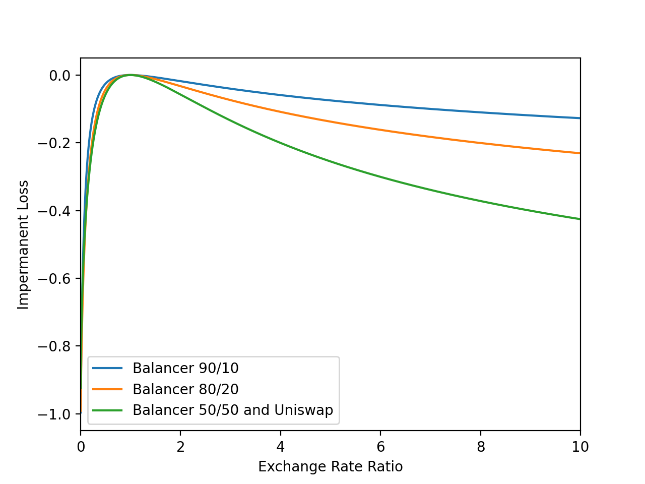
Along these lines, we start by observing and codifying some of the properties of G3Ms. The major property that we focus on in this paper is what we call Exchange Rate Level Independence (ERLI). This property states that impermanent loss can be understood entirely in terms of ratios of initial and final exchange rates, as opposed to the actual rates themselves. In other words, moving from an Eth BTC exchange rate of to an exchange rate of has the same effect on impermanent loss as moving from an exchange rate of to an exchange rate of , since in both scenarios the exchange rate has doubled. G3Ms exhibit this property, though to our knowledge, it has not been clearly formalized for higher dimensional AMMs until now. Among other conceptual benefits, exchange rate level independence allows us to analyze impermanent loss for AMMs with fewer parameters.
Showing that G3Ms (up to a simple transformation) have the ERLI property and are the only AMMs to have this property is the main result of this paper. The connection between portfolio value functions and trading functions pointed out in [AEC21] is a crucial first step towards establishing this result. However, a slightly different viewpoint is used in this paper. We focus on individual level surfaces of an AMM as opposed to the function that generates them. The following example might motivate this shift in focus. Consider
Both of these functions have the same level curves, namely the liquidity curves of Uniswap, but only the first function is a geometric mean market maker. As such, trying to infer properties of from its impermanent loss characteristics is misguided since both the above market makers would lead to the same impermanent loss. On the other hand, restricting a priori to the class of geometric mean market makers precludes some interesting AMMs like Curve’s StableSwap. Focusing on the level surfaces of has conceptual benefits as well, some of which are outlined in Section 5.
Readers familiar with the space can skip to Section , in which we derive an impermanent loss formula for higher dimensional constant product market makers. In the process of doing so, we note that these constant product market makers have some helpful properties that we work to concretize in the later sections. We then show that the smallest class of market makers with these properties is the class of market makers whose level surfaces match those of a geometric mean market maker.
2 Background and Notation
In what follows, we will use a definition for an automated market maker (AMM) motivated by [EH21].
Definition 1.
An automated market maker is a map where
-
1.
-
2.
for all
-
3.
is strictly convex for all .
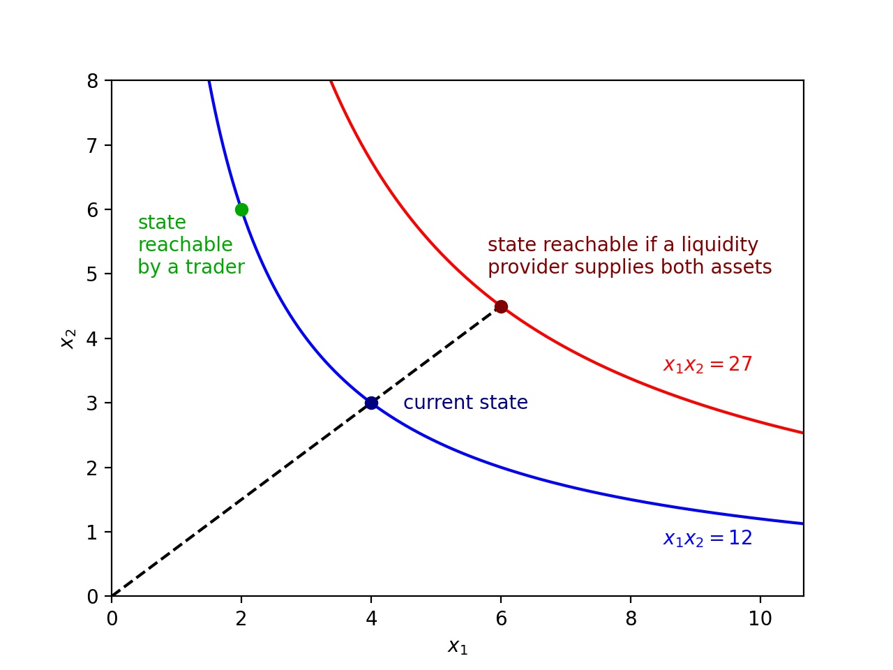
Note that some authors require that the AMM is homogeneous (i.e. for some ) while other authors don’t; see [CJ21] and [EH21] respectively. In practical terms, an AMM provides a programmatic way for traders to swap tokens for one another. In the above definition, represents the number of tokens, and is the quantity of token . For a given state of quantities , there is a level surface (or curve if ) of that passes through this state. Traders are allowed to swap tokens in and out of the AMM in any manner that leaves the resulting state on the surface . In contrast, liquidity providers through their actions can move the state from one level surface to another. The first condition ensures smoothness of these surfaces, the second condition ensures that the level surfaces are sensibly indexed, and the third condition ensures that the level surfaces are convex. It is worth mentioning that the commonly presented two-dimensional hyperbolic constant product market makers correspond to the function , some of whose level curves are pictured below. For a more thorough introduction to these ideas, consult [AC20].
A price vector assigns a price to each token so that is the price of token in terms of some measuring currency. A price vector can be thought of in state space as the gradient vector (it points in the direction of steepest increase) of the value function
This value function is naturally defined in that it is the sum of the product of each token quantity by the corresponding token price. If we think of as a function on the state space (given a fixed price vector ), we see that has a constant gradient . We see in Figure 3 the relationship between the price vector and the level curves of the value function that it induces.
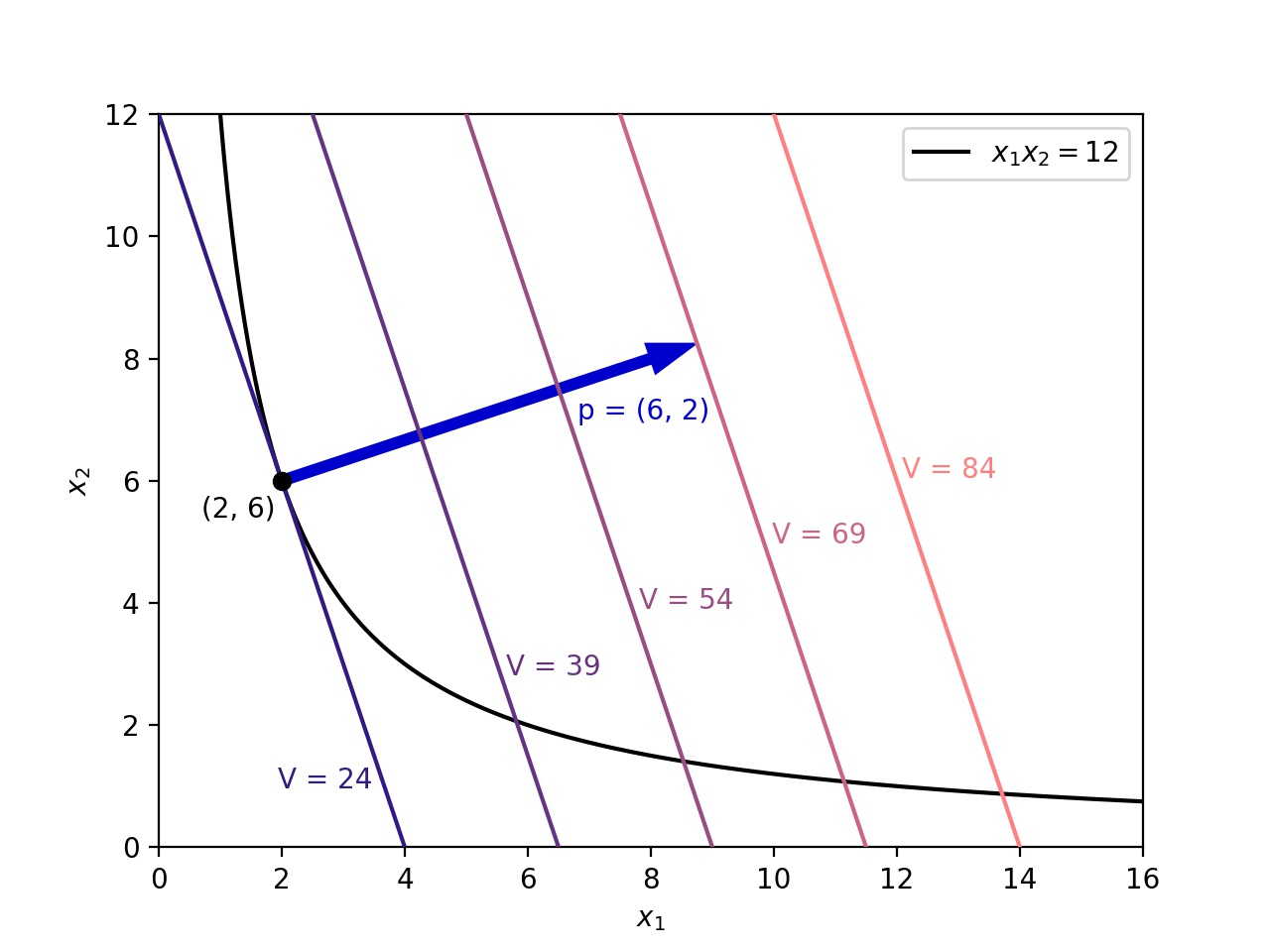
In Figure 3, the state is referred to as a stable point, in that it is the state with the lowest value on the current trading curve . We will define stable points more formally below. Note that the measuring currency is not important in the context of defining stable points. Changing the measuring currency through which is defined would stretch or contract , but it would not change its direction. Also, changing the measuring currency would leave the family of level curves (surfaces) intact, though it would alter the values corresponding to these level curves (surfaces). If, for instance, the measuring currency were taken to be the first token, would be and would be , which would result in the same level curves for the value function as shown in Figure 3, but with the corresponding values divided by .
Let’s make a fixed choice of price , AMM , and number . We say that a point is stable if
In other words, a state is stable if it has the lowest value among all states on the level surface that it defines. This corresponds to the idea that arbitrageurs will drive the AMM state to this stable state based on the external market valuation of the assets. Finding such a stable point is a Lagrange multipliers problem; we are trying to minimize the value of subject to the condition that . We know that and therefore must be parallel to evaluated at the given state. For instance, in Figure 3 one can observe that the gradient of at the stable point is parallel to .
In what follows, we assume that if the price vector changes (one can think of it as fluctuating exogenously), the state vector in the AMM changes to the corresponding stable point (thanks to arbitrageurs). In [EH21], it is shown that for a given price vector , there is a unique stable point on the surface. In other words, the stable state is a function of price
but we will avoid using this notation to keep the exposition clean. Suppose that the price vector changes from to . The following definition helps to quantify the loss liquidity providers face when compared to those who simply hold their assets. It is commonly referred to in the literature as impermanent loss or divergence loss.
Definition 2.
Fix an AMM and a level surface . Suppose the initial and final prices are given by and , and that the corresponding stable states are and . Then the impermanent loss is defined to be
Note that the above formula for impermanent loss is dependent on since is a function of . Thus, impermanent loss at first glance seems to be a function of and , which involves parameters. In the next section, we will investigate whether we can in general reduce the number of parameters needed to compute impermanent loss. To provide context for this investigation, we will conclude this section with a simple example. We will derive the well known formula for the impermanent loss of a two dimensional constant product market maker.
Example 3.
For a constant product market maker with two assets and where , consider two assets with initial prices and , initial quantities and , final prices and , and final quantities and . The impermanent loss formula given by
Proof.
Before we prove the statement, we will provide intuition for what signifies. We first define to be the exchange rate between tokens and , so that is the price of token in terms of token . Concretely, and . The parameter is the quotient of the final and initial exchange rates. The further is away from , the more drastically the exchange rate between the tokens has changed.
To prove the claim, we can start by expressing the quantities in terms of prices. As noted above, with the assumption that arbitrageurs will drive the value of the pool to a minimum, we can use Lagrange multipliers to find the stable state as a function of . We see that , so solving
yields and . Substituting this back into the original equation, we get
Dividing the numerator and denominator by , we get
Using the definition that , we obtain
Finally, letting , we arrive at the desired result. ∎
As is well known, the above formula demonstrates that impermanent loss is least destructive when , that is when the exchange rate between tokens does not change (here ). The key takeaway that we will try to generalize in what follows is that impermanent loss is best understood in terms of this one parameter , as opposed to the four parameters , , and .
3 Higher Dimensional Constant Product Market Makers
To gain an intuition for the parameters that should be used to conceptualize impermanent loss in higher dimensions, we start by proving a theorem involving an dimensional constant product market maker.
Theorem 4.
Consider a constant product market maker with assets where
Let the initial prices of the assets be given by , initial quantities , final prices , and final quantities . The impermanent loss formula given by
Proof.
We again start by expressing the quantities in terms of prices. To do so, similarly as in Example 3, we must solve the Lagrange multipliers equations:
Multiplying the first equations leads to the equation
and so
Thus, . Dividing the last of the Lagrange multiplier (the constraint equation) by the equation yields
Since the impermanent loss formula involves expressions, it is convenient to note that
This demonstrates that the stable state for a constant product market maker occurs when each collection of tokens in the AMM has the same value. Substituting this back into the original equation, we get
We now introduce the analogs to the exchange rates in Example 3 by defining , so that is the exchange rate between tokens and . Then, we see that
Thus, noting that yields the final result:
∎
Similarly to Example 3, is the quotient of the final exchange rate and initial exchange rate between assets and . The fact that the for constant product market makers is a direct consequence of the arithmetic mean-geometric mean inequality applied to these exchange rate quotients. Again, the key takeaway is that impermanent loss is best understood in terms of these parameters, not the price parameters. This result has important economic implications in addition to its overall simplifying nature.
The parameter reduction in the impermanent loss formula from initial prices and final prices to quotients of exchange rates can be decomposed into two parts. The first reduction consists of using relative pricing of one asset against another as opposed to the raw prices (in our case, we have been pricing assets in terms of the first asset). This is typically referred to as numeraire independence in finance, but we will refer to it as price level independence. The next reduction takes us from separate relative initial and final exchange rates to quotients of final and initial exchange rates. We call this exchange rate level independence, since the absolute levels of the initial and final exchange rates do not matter, only the quotients. In the next section, we will show that impermanent loss for all AMMs exhibits price level independence, but not necessarily exchange rate level independence.
4 Price Level Independence
The goal of this section is to generalize the above idea of reducing the number of parameters involved in defining impermanent loss. We will begin by showing that impermanent loss for all AMMs is price level independent. Price level independence is intuitive and not particularly deep in its own right, but we wish to build towards understanding exchange rate level independence systematically. To this end, we need the following lemma, which formalizes the concept introduced in the background section that rescaling price vectors does not affect stable points. In this section, we think of there being a fixed measuring currency through which and hence are defined. In other words, corresponds to a world in which all prices have doubled, not one in which the measuring currency has changed.
Lemma 5.
Let be an AMM and for fixed , consider the liquidity surface . We know that we can express the stable point on the surface as a function of price : . The function is homogeneous of degree in . In other words,
for all , and so stable points are price level independent.
Proof.
Fix a price vector and . Let . Then, satisfies the following Lagrange multiplier equations:
for some . It follows that satisfies
for . By uniqueness of stable points, . ∎
Price level independence for the impermanent loss of an AMM follows immediately.
Theorem 6.
The impermanent loss of an AMM exhibits price level independence. In other words, impermanent loss can be expressed entirely in terms of exchange rates of tokens relative to the first token (or any token for that matter).
Proof.
where the last equality follows from the lemma. Using our previous notation and defining , we obtain
∎
Indeed, it is clear from the proof that we could express impermanent loss using exchange rates relative to any fixed asset. Along these lines, it will be convenient at times to change the base token from the first token to another of the tokens. In other words, we might define
so that we use the token as the base token when computing exchange rates. In this case, . To keep the notation uncluttered, though, we will suppress the and make sure that it is clear from context when important.
Example 7.
We will give context for the price level independence of impermanent loss through an example involving a two dimensional AMM . We make no assumptions about the specific formula for this AMM and we investigate a fixed liquidity curve . The price vectors and are perpendicular to the liquidity curve at the initial and final stable states and respectively. The above theorem formalizes the idea that impermanent loss can be understood using slopes alone. In other words, the sizes of the price vectors and are irrelevant. If we use the second token as the base token, we see that the normalized versions of and are and respectively. Thus, in two dimensions, each price vector is associated to a slope as is pictured, and these slopes are the negatives of the exchange rates. Instead of the four parameters , , , and , we only need two parameters: and . Refer to Figure 4 for visualization.
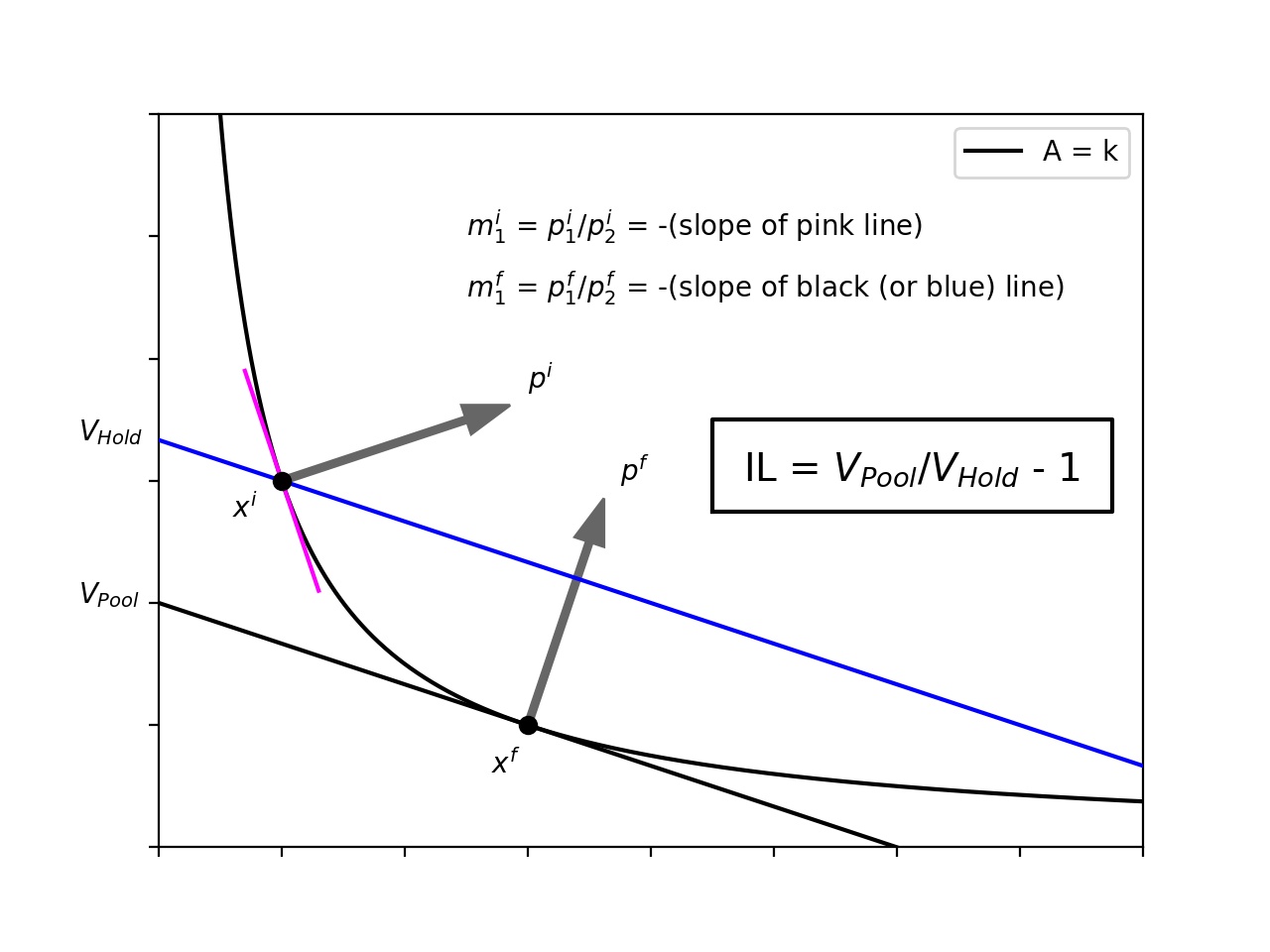
Another way of interpreting Theorem 6 is that impermanent loss is agnostic to the measuring currency used for both and . Indeed, we could use a different measuring currency for and without affecting impermanent loss, though we will not do this. The above figure offers some insight into how we can choose the measuring currency so that can be gleaned geometrically. More concretely, if the token is the measuring currency, the pool value is the intercept111We could use any of the tokens as the measuring currency, and then the pool value would be the corresponding intercept value. of the line with the following properties:
-
•
passes through the current pool state
-
•
is perpendicular to
The slope of is the negative of the exchange rate between the two tokens. This line will be tangent to the curve if the pool state is the current stable state. In the above example, if the individual had just held their assets, the value of their assets would have been equivalent to the value of tokens. By providing liquidity, the value of their assets is instead tokens. This diagram makes it clear why the convexity condition for AMMs ensures that impermanent loss will always be negative.
5 The Legendre Transform and the Connection Between Value and State
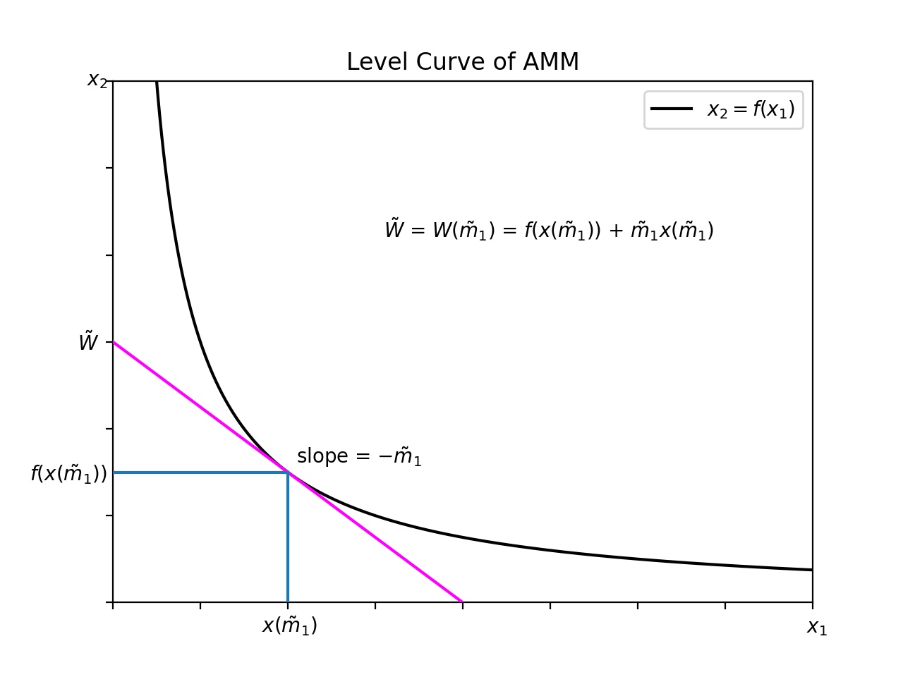
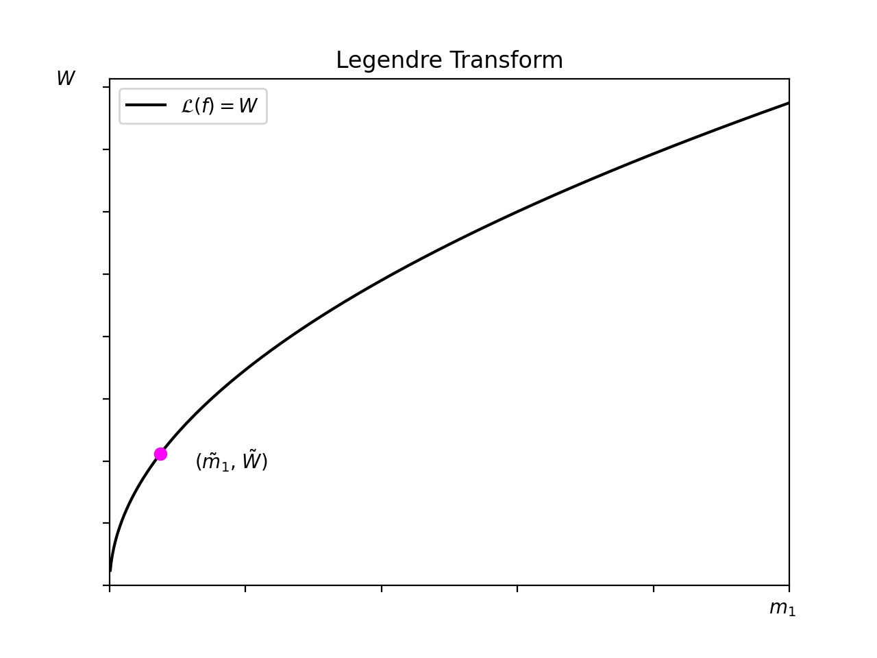
As introduced in [AEC21], there is an elegant mathematical relationship between automated market makers and their corresponding portfolio value functions. In that paper, the relationship is formulated between the AMM and its value function via the Legendre-Fenchel transform. Example 7 motivates us to proceed a bit differently. The core object that we will work with instead of is , which we will define as the function that defines the specific level curve (or surface) :
For those looking for a visual encapsulation of this section, and possibly to skip some of the rigmarole, the graphs at the end of this section illustrate the main ideas.
By our AMM assumptions and the implicit function theorem, is a continuously differentiable surface. Henceforth, we will use the token as the measuring currency through which and hence are defined. In other words, and is the exchange rate between token and token for . To maintain consistency with the previous section, we will use to reference these exchange rates. Define as
and define
In other words, given the exchange rates , a unique stable point is determined, and is the value of the corresponding stable portfolio. We will use interchangeably with , mainly to simplify notation and to avoid introducing new notation. From Example 7, we see that . In other words, at stable points, we can obtain the exchange rate as the negative derivative of 222In Example 7, is the stable point at the final exchange rate , while is not a stable point.. The following lemma proves and generalizes this observation to cases in which is a function of exchange rates.
Lemma 8.
With and for defined as above, we have that
Proof.
For the stable point , we have the Lagrange multiplier equations
for some . Differentiating the relation
with respect to yields
Substituting into the above yields
and so the result is proved. ∎
The next lemma frames the same relationship from the viewpoint that the are functions of the .
Lemma 9.
With defined as above and the functions for defined as the natural inverses to the functions, we have that
Proof.
The following theorem gives a precise formulation of how and are dual functions. For readers unfamiliar with the Legendre transform, the remainder of the paper is self-contained: all properties that we need are readily derived from the formulas that we have established. As such, the following theorem is just a form of mental bookkeeping. We recommend [ZRM09] as a useful resource to learn more about the Legendre transform and its applications.
Theorem 10.
Denote the Legendre transform of a function in all of its variables as . In other words,
where is defined as
We then have that
Proof.
The result follows from Lemma 8. ∎
Again, the relationship between and via the Legendre-Fenchel transform was pointed out in [AEC21], and this observation accounts for the heavy lifting. It can be cumbersome in some settings, however, to think in terms of (a family of level curves or surfaces) as opposed to the single AMM surface given by . For instance, to replicate a payoff function , one can extend to via 1-homogeneity, transform via the Legendre-Fenchel transform into an , and then manipulate to obtain a more amenable AMM form . Alternatively, one can use Theorem 10 to pass from to directly. The graphs in Figure 5 illustrate the relationship between and in two dimensions.
 |
 |
6 Exchange Rate Level Independence
In general, price level independence of impermanent loss allows us to reduce the number of parameters from to . When we derived the impermanent loss formula for the -dimensional constant product market maker, however, we were able to reduce the number of relevant parameters even further to . These parameters were quotients of the initial and final exchange rates (relative to a fixed token).
Definition 11.
Let be an AMM and fix a liquidity surface . Let be price vectors and denote the corresponding stable states . Define and . We say that the AMM is exchange rate level independent (i.e. ERLI) if can be rewritten as a function of the exchange rate quotients (where can be omitted because it is always equal to ).
In other words, the AMM satisfies the ERLI conditions if its impermanent loss can be written purely as a function of exchange rate quotients. Before proceeding, let us consider an example that does not meet this requirement.
Example 12.
The Curve StableSwap AMM introduced in [Ego19] does not satisfy the ERLI condition. We will demonstrate this by using their proposed two dimensional AMM with parameter (not to be confused with the that we have been using to denote our AMM). The level curve of this AMM (where we use the notation from the paper) is given by
which can be simplified to
Note that
is not homogeneous in . There is a better way to see this without solving for . Assume for a contradiction that for some . Then,
for all and some nonzero constants and . This is impossible since the term will grow unchecked in . In this section, we will show that the lack of homogeneity of implies that the impermanent loss function for this liquidity curve does not satisfy the ERLI condition.
Our first goal will be to write impermanent loss in terms of the value function defined in the previous section. To this end, we need the following lemma. We warn the reader of the notational simplification
and define and as in the previous section.
Lemma 13.
For , we have
Proof.
We start with relation
and differentiate both sides of the equality with respect to to obtain
which yields the result since
for . ∎
We are now ready to recast impermanent loss in terms of .
Theorem 14.
The expression for impermanent loss in terms of is
where is the linear approximation to at .
We will finish the section by providing a necessary and sufficient condition on for its impermanent loss to satisfy the ERLI condition. To this end, we need a lemma that connects the homogeneity properties of to the homogeneity properties of .
Lemma 15.
The following two statements are equivalent.
-
1.
For each , is homogeneous of degree in .
-
2.
For each , is homogeneous of degree in .
Furthermore,
Note that the case that is precluded by the condition that the AMM is strictly convex333To see this, consider the straight line parametric path in given by , for . If , then for some constant . Fix . For any points and falling on , . .
Proof.
From the way that was originally defined, it is clear that is the solution to the following value minimization problem
Assume that the first statement holds. Then, with defined as in the statement of the theorem,
Thus, we have shown that statement implies statement . For the other direction, we note that
| (1) |
To see this, we can unpack the meanings of and . Fix as the quantities for tokens through in the AMM. Then: is the overall value in the AMM (measured in tokens) at the stable point corresponding to exchange rate vector , and is the value of tokens tokens through (measured in tokens) assuming exchange rate vector . Thus, is maximized by the exchange vector that allows for the most tokens. This exchange rate vector corresponds to the world with the most profitable “hold” strategy. There are other more technical ways to show that above equation holds, but we omit these for expository flow. Using equation (1), we can prove the other direction of the lemma in an analogous manner to the first direction. ∎
We need two final lemmas relating the homogeneity of to the homogeneity of before proceeding with the final theorem of this section.
Lemma 16.
If is homogeneous in each of its coordinates, then is homogeneous in each of its inputs.
Proof.
Assume that is homogeneous of degree in for all . Then,
implying by uniqueness that
∎
Lemma 17.
Assume for each , the function induced by is homogeneous in each of its coordinates444Technically, should be subscripted by , but we drop the to simplify notation.. Then, there is a function that is homogeneous in each of its coordinates and such that , where is a smooth function of one variable.
Proof.
For a fixed , assume that is homogeneous of degree for . We start with
and proceed to obtain
where for . Observe that all level surfaces can be expressed using the same exponents since, otherwise, the level surfaces would cross. In other words, setting two surface equations like the one above with different ’s equal to one another would lead to solutions:
Define . Then and have the same level surfaces and can be defined accordingly. ∎
We are now ready to state a necessary and sufficient condition on that ensures that its impermanent loss will satisfy the ERLI condition.
Theorem 18.
Let be an AMM. Then , where is a smooth function of one real variable and is homogeneous in each coordinate if and only if the formula for impermanent loss is ERLI for every liquidity surface .
Proof.
We start with the forward direction. Fix . Without loss of generality, we can assume that is homogeneous in each coordinate since corresponds to some . By Lemma 16, is homogeneous in each of its coordinates, and so then by Lemma 15, is homogeneous in each of its coordinates. Say that is homogeneous of degree in . Defining for and invoking Theorem 14, we have
where in the second equality we have used the fact that is homogeneous of degree in if and is homogeneous of degree in . Thus, noting that IL has been expressed entirely in terms of the exchange rate ratios , the forward direction is complete.
Fix and consider the surface with induced function . For the reverse direction, by Lemma 17, it suffices to show that is homogeneous in each of its coordinates. By Lemma 15, it then suffices to show that is homogeneous in each of its coordinates. Choose a coordinate and fix . Fix all other coordinates aside from in defining the following functions:
The fact that impermanent loss is ERLI for the surface implies that
for all . Thus, substituting and yields
which simplifies to
with . Defining , we obtain the ODE
This is a simple separable ODE with solutions of the form
for constant 555 might depend on for .. Note that even though the ODE has a singularity at , from its direction field, it is clear that the only differentiable functions that satisfy it are of this form. Using the fact that the equation holds, we conclude that and hence that
| (2) |
The homogeneity of in will follow from this equation, but there is a bit more work to do to see this. Since depends on , we have established that
for some function . It turns out that this is enough to show that is homogeneous since satisfies the property :
Thus, is a solution to Cauchy’s multiplicative functional equation and this implies that for some . For more background on such equations, consult [Kuc09].
Note that we are still not quite done. We have shown that , but our may in theory depend on the for . To see that this is not the case, fix two vectors and in . We know that
The fact that impermanent loss is ERLI for the surface implies that
Absorbing terms depending on and into constants yields
and once more simplified, an equation of the form
where the s and s are constants that depend on the s and s. By the strict concavity of (established by the relation in Lemma 15), it is clear that , , , and are nonzero. As such, for the above equation to hold for all , , , and
∎
The following corollaries are useful when it is not immediately obvious whether is of the form with homogeneous in each of its coordinates.
Corollary 19.
Let be an AMM. Let be a liquidity surface and let be the function that it induces. Then is homogeneous in each of its coordinates if and only if the impermanent loss for is ERLI.
Corollary 20.
Geometric mean market makers and compositions of these market makers with smooth real valued functions compose the space of ERLI market makers.
7 Conclusion
In this paper, we have established a framework for reducing the parameters involved in describing impermanent loss for automated market makers. In doing so, we have shown that geometric mean market makers are the simplest class of market makers from an impermanent loss standpoint. More concretely, G3Ms exhibit a condition that we call Exchange Rate Level Independence (ERLI). ERLI is an interesting property in that it is connected to how the dynamics of AMMs are affected when token quantities are rescaled. Such rescalings can be done for either conceptual or computational purposes. An example of this sort of rescaling transformation can be found in the Curve V2 whitepaper [Ego21] and we believe that this mechanism also shifts Curve V2’s impermanent loss profile to a new profile that is closer to having ERLI. We will work to quantify this in future work, and more generally, we are interested in exploring how to extend our framework to dynamic AMMs.
8 Acknowledgements
The authors would like to thank Jamie Irvine for several interesting conversations and for his insight regarding a critical lemma in this paper. We would also like to thank Austin Pollok for sharing his insights regarding parallels between DeFi and TradFi. Finally, we would like to thank Guillermo Angeris for sharing his ideas and useful feedback with us.
References
- [AC20] Guillermo Angeris and Tarun Chitra. Improved price oracles: Constant function market makers. In Proceedings of the 2nd ACM Conference on Advances in Financial Technologies, pages 80–91, 2020.
- [AD21] Andreas A Aigner and Gurvinder Dhaliwal. Uniswap: Impermanent loss and risk profile of a liquidity provider.arXiv preprint arXiv:2106.14404, 2021.
- [Ada18] Hayden Adams. Uniswap whitepaper. URL: https://hackmd.io/C-DvwDSfSxuh-Gd4WKEig, 2018.
- [AEC20] Guillermo Angeris, Alex Evans, and Tarun Chitra. When does the tail wag the dog? Curvature and market making. arXiv preprint arXiv:2012.08040, 2020.
- [AEC21] Guillermo Angeris, Alex Evans, and Tarun Chitra. Replicating market makers, 2021.
- [Aoy20] Jun Aoyagi. Liquidity provision by automated market makers. Available at SSRN 3674178,2020.
- [Bou21] Nassib Boueri. G3m impermanent loss dynamics. arXiv preprint arXiv:2108.06593, 2021.
- [CJ21] Agostino Capponi and Ruizhe Jia. The adoption of blockchain-based decentralized exchanges, 2021.
- [Ego19] M. Egorov. Stableswap-efficient mechanism for stablecoin liquidity. Tech. Rep., 2019.
- [Ego21] M. Egorov. Automatic market-making with dynamic peg., 2021.
- [EH21] Daniel Engel and Maurice Herlihy. Composing networks of automated market makers. CoRR, abs/2106.00083, 2021.
- [Eva20] Alex Evans. Liquidity provider returns in geometric mean markets. arXiv preprint arXiv:2006.08806, 2020.
- [Kuc09] Marek Kuczma. An introduction to the theory of functional equations and inequalities. 01 2009.
- [MM19] Fernando Martinelli and Nikolai Mushegian. Balancer whitepaper. URL: https://balancer.fi/whitepaper.pdf, 2019.
- [ZRM09] R. K. P. Zia, Edward F. Redish, and Susan R. McKay. Making sense of the Legendre transform. American Journal of Physics, 77(7):614–622, Jul 2009.