A general framework of rotational sparse approximation in uncertainty quantification
Abstract
This paper proposes a general framework to estimate coefficients of generalized polynomial chaos (gPC) used in uncertainty quantification via rotational sparse approximation. In particular, we aim to identify a rotation matrix such that the gPC expansion of a set of random variables after the rotation has a sparser representation. However, this rotational approach alters the underlying linear system to be solved, which makes finding the sparse coefficients more difficult than the case without rotation. To solve this problem, we examine several popular nonconvex regularizations in compressive sensing (CS) that perform better than the classic approach empirically. All these regularizations can be minimized by the alternating direction method of multipliers (ADMM). Numerical examples show superior performance of the proposed combination of rotation and nonconvex sparse promoting regularizations over the ones without rotation and with rotation but using the convex approach.
keywords: Generalized polynomial chaos, uncertainty quantification, iterative rotations, compressive sensing, alternating direction method of multipliers, nonconvex regularization .
1 Introduction
A surrogate model (also known as “response surface”) plays an important role in uncertainty quantification (UQ), as it can efficiently evaluate the quantity of interest (QoI) of a system given a set of inputs. Specifically, in parametric uncertainty studies, the input usually refers to a set of parameters in the system, while the QoI can be observables such as mass, density, pressure, velocity, or even a trajectory of a dynamical system. The uncertainty in the system’s parameters typically originates from the lack of physical knowledge, inaccurate measurements, etc. Therefore, it is common to treat these parameters as random variables, and statistics, e.g., mean, variance, and the probability density function (PDF) of the QoI with respect to such random parameters are crucial in understanding the behavior of the system.
The generalized polynomial chaos (gPC) expansion [23, 58] is a widely used surrogate model in applied mathematics and engineering studies, which uses orthogonal polynomials associated with measures of the aforementioned random variables. Under some conditions, the gPC expansion converges to the QoI in a Hilbert space as the number of polynomials increases [9, 21, 42, 58]. Both intrusive methods (e.g., stochastic Galerkin) and non-intrusive methods (e.g., probabilistic collocation method) [4, 23, 52, 57, 58] have been developed to compute the gPC coefficients. The latter is particularly more desirable to study a complex system, as it does not require to modify the computational models or simulation codes. For example, the gPC coefficients can be calculated based on input samples and corresponding output using least squared fitting, probabilistic collocation method, etc.
However, in many practical problems, it is prohibitive to obtain a large amount of output samples used in the non-intrusive methods, because it is costly to measure the QoI in experiments or to conduct simulations using a complicated model. Consequently, one shall consider an under-determined linear system (matrix), denoted as , of size with (or even ), where is the size of available output samples and is the number of basis functions used in the gPC expansion. When the solution to the under-determined system is sparse, compressive sensing (CS) techniques [8, 10, 11, 19] are effective. Recent studies have shown some success in applying CS to UQ problems [2, 20, 33, 34, 44, 49, 60, 61, 64]. For example, sampling strategies [3, 27, 30, 46] can improve the property of to guarantee sparse recovery via the minimization. Computationally, the weighted minimization [1, 13, 43, 47, 64] assigns larger weights to smaller components (in magnitude) of the solution, and hence minimizing the weighted norm leads to a sparser solution than the vanilla minimization does. Besides, adaptive basis selection [3, 6, 16, 28, 29] as well as dimension reduction techniques can be adopted to reduce the number of unknown variables [55, 67] thus improving computational efficiency.
In this paper, we focus on a sparsity-enhancing approach, referred to as iterative rotation [34, 65, 66, 68], that intrinsically changes the structure of a surrogate model to make the gPC coefficients more sparse. However, this method tends to deteriorate properties of that are favorable by CS algorithms, e.g., low coherence, which may counteract the benefit of the enhanced sparsity. Since the polynomials in the gPC expansion may not be orthogonal after the rotation of the random variables, the coherence of may not converges to zero asymptotically, leading to an amplified coherence after the rotation. To remedy this drawback, we innovatively combine the iterative rotation technique with a class of nonconvex regularizations to improve the efficiency of CS-based UQ methods. Specifically, our new approach uses rotations to increase the sparsity while taking advantages of the nonconvex formalism for dealing with a matrix that is highly coherent. In this way, we leverage the advantages of both methods to exploit information from limited samples of the QoI more efficiently and to construct gPC expansions more accurately. Main contributions of this work are two-fold. On one hand, we propose a unified and flexible framework that combines iterative rotation and sparse recovery together with an efficient algorithm. On the other hand, we empirically validate a rule of thumb in CS that nonconvex regularizations often lead to better performance compared to the convex approach.
The rest of the paper is organized as follows. We briefly review gPC, CS, and rotational CS in 2. We describe the combination of sparse signal recovery and rotation matrix estimation in 3. 4 devotes to numerical examples, showing that the proposed approach significantly outperforms the state-of-the-art. Finally, conclusions are given in 5.
2 Prior works
In this section, we briefly review gPC expansions, useful concepts in CS, and our previous work [65, 68] on the rotational CS for gPC methods.
2.1 Generalized polynomial chaos expansions
We consider a QoI that depends on location , time and a set of random variables with the following gPC expansion:
| (1) |
where and denotes the truncation error. Here, are orthonormal with respect to the measure of , i.e.,
| (2) |
where is the PDF of , is the Kronecker delta function, and we usually set . We study systems relying on -dimensional i.i.d. random variables and the gPC basis functions are constructed by tensor products of univariate orthonormal polynomials associated with . Specifically for a multi-index with each , we set
| (3) |
where are univariate orthonormal polynomial of degree . For two different multi-indices and , we have
| (4) |
with Typically, a th order gPC expansion involves all polynomials satisfying for , which indicates that a total number of polynomials are used in the expansion. For simplicity, we reorder in such a way that we index by , which is consistent with Eq. (1).
In this paper, we focus on time independent problems, in which the gPC expansion at a fixed location is given by
| (5) |
where each is a sample of , e.g, , and is the number of samples. We rewrite the above expansion in terms of the matrix-vector notation, i.e.,
| (6) |
where is a vector of output samples, is a vector of gPC coefficients, is an matrix with and is a vector of errors with . We are interested in identifying sparse coefficients among the solutions of an under-determined system with in (6), which is the focus of compressive sensing [12, 17, 22].
2.2 Compressive sensing
We review the concept of sparsity, which plays an important role in error estimation for solving the under-determined system (6). The number of non-zero entries of a vector is denoted by . Note that is named the “ norm” in [17], although it is not a norm nor a semi-norm. The vector is called -sparse if , and it is considered a sparse vector if . Few practical systems have truly sparse gPC coefficients, but rather compressible, i.e., only a few entries contributing significantly to its norm. To this end, a vector is defined as the best -sparse approximation which is obtained by setting all but the -largest entries in magnitude of to zero, and subsequently, is regarded as sparse or compressible if is small for .
In order to find a sparse vector from (6), one formulates the following problem,
| (7) |
where is a positive parameter to be tuned such that As the minimization (7) is NP-hard to solve [41], one often uses the convex norm to replace , i.e.,
| (8) |
A sufficient condition of the minimization to exactly recover the sparse signal was proved based on the restricted isometry property (RIP) [11]. Unfortunately, RIP is numerically unverifiable for a given matrix [5, 53]. Instead, a computable condition for ’s exact recovery is coherence, which is defined as
| (9) |
Donoho-Elad [18] and Gribonval [24] proved independently that if
| (10) |
then is indeed the sparsest solution to (8). Although the inequality condition in (10) is not sharp, the coherence of a matrix is often used as an indicator to quantify how difficult it is to find a sparse vector from a linear system governed by in the sense that the larger the coherence is, the more challenging it is to find the sparse vector [37, 70]. Apparently if the samples are drawn independently according to the distribution of , for the gPC expansion converges to zero as [20]. However, the rotation technique tends to increase the coherence of the matrix, leading to unsatisfactory performance of the subsequent minimization as discussed in [68].
In this work, we promote the use of nonconvex regularizations to find a sparse vector when the coherence of is relatively large, referred to as a coherent linear system. There are many nonconvex alternatives to approximate the norm that give superior results over the norm, such as [14, 59, 32], capped [73, 50, 38], transformed [39, 71, 72, 25], - [69, 37, 36], [45, 56] and error function (ERF) [26]. We formulate a general framework that works for any regularization whose proximal operator can be found efficiently. Recall that a proximal operator of a functional is defined by
| (11) |
where is a positive parameter. We provide the formula of aforementioned regularizations together with their proximal operators as follows,
-
•
The norm of is with its proximal operator given by
(12) where denotes the Hadamard operator for componentwise operation.
-
•
The square of the norm is defined as whose proximal operator [59] is expressed as
(13) where and the square is also computed componentwisely.
-
•
Transformed (TL1) is defined as for a positive parameter and its proximal operator [71] is given by
(14) with
-
•
The - regularization is defined by and its proximal operator [36] is given by the following cases,
-
–
If , one has , where .
-
–
If , is an optimal solution if and only if for , and for all . The optimality condition implies infinitely many solutions of among which we choose for the smallest satisfies and the rest coefficients set to be zero.
-
–
-
•
The error function (ERF) [26] is defined by
(15) for . Though there is no closed-form solution for this problem, one can find the solution via the Newton’s method. In particular, the optimality condition of (11) for ERF reads as
When , we have . Otherwise the optimality condition becomes
which can be found by the Newton’s method.
2.3 Rotational compressive sensing
To further enhance the sparsity, we aim to find a linear map such that a new set of random variables given by
| (16) |
leads to a sparser polynomial expansion than does. We consider as an orthogonal matrix, i.e., with the identity matrix , such that the linear map from to can be regarded as a rotation in . Therefore, the new polynomial expansion for is expressed as
| (17) |
Here can be understood as a polynomial evaluated at random variables , and the same for . Ideally, is sparser than . In the previous works [34, 65], it is assumed that , so . For general cases where are not i.i.d. Gaussian, are not necessarily independent. Moreover, are not necessarily orthogonal to each other with respect to . Therefore, may not be a standard gPC expansion of , but rather a polynomial equivalent to with potentially sparser coefficients [68].
We can identify using the gradient information of based on the framework of active subspace [15, 48]. In particular, we define
| (18) |
Note that is a matrix, and we consider in this work. The singular value decomposition (SVD) of yields
| (19) |
where is a orthogonal matrix, is a matrix, whose diagonal consists of singular values , and is an orthogonal matrix. We set the rotation matrix as . As such, the rotation projects to the directions of principle components of . Of note, we do not use the information of the orthogonal matrix .
Unfortunately, is unknown, and thus the samples of are not available. Instead, we approximate Eq. (18) by a computed solution that can be obtained by the minimization [65]. In other words, we have
| (20) |
and the rotation matrix is constructed based on the SVD of :
| (21) |
Defining we compute the corresponding input samples as and construct a new measurement matrix as . We then solve the minimization problem in Eq. (8) to obtain . If some singular values of are much larger than the others, we can expect to obtain a sparser representation of with respect to which is dominated by the eigenspace associated with these larger singular values. On the other hand, if all the singular values are of the same order, the rotation does not enhance the sparsity. In practice, this method can be designed as an iterative algorithm, in which and are updated separately following an alternating direction manner.
It is worth noting that the idea of using a linear map to identify a possible low-dimensional structure is also used in sliced inverse regression (SIR) [35], active subspace [15, 48], basis adaptation [54], etc., but with different manners in computing the matrix. In contrast to these methods, the iterative rotation approach does not truncate the dimension in the sense that is a square matrix. As an initial guess may not be sufficiently accurate, reducing dimension before the iterations terminate may lead to suboptimal results. The dimension reduction was integrated with an iterative method in [62], while another iterative rotation method preceded with SIR-based dimension reduction was proposed in [67]. We refer interested readers to the respective literature.
3 The proposed approach
When applying the rotational CS techniques, the measurement matrix may become more coherent compared with . This is because popular polynomials used in gPC method, e.g., Legendre and Laguerre polynomials, are not orthogonal with respect to the measure of , so converges to a positive number instead of zero as does. Under such a coherent regime, we advocate the minimization of a nonconvex regularization to identify the sparse coefficients.
To start with, we generate input samples based on the distribution of and select the gPC basis functions associated with in order to generate the measurement matrix by setting as in Eq. (6), while initializing and Then we propose an alternating direction method (ADM) that combines the nonconvex minimization and rotation matrix estimation. Specifically given and we formulate the following minimization problem,
| (22) |
where denotes a regularization functional and is a weighting parameter. For example, our early work [65] considered , i.e., the approach. We can minimize Eq. (22) with respect to and in an alternating direction manner. When is fixed, we minimize a sparsity-promoting functional to identify the sparse coefficients as detailed in Section 3.1. When is fixed, optimizing is computationally expensive, unless a dimension reduction technique is used, e.g., as in [55]. Instead, we use the rotation estimation introduced in Section 2.3 to construct . Admittedly, this way of estimating may not be optimal, but it can potentially promote the sparsity of , thus improving the accuracy of the sparse approximation of the gPC expansion.
3.1 Finding sparse coefficient via ADMM
We focus on the -subproblem in (22), whose objective function is defined as
| (23) |
We adopt the alternating direction method of multipliers (ADMM) [7] to minimize (23). In particular, we introduce an auxiliary variable and rewrite (23) as an equivalent problem,
| (24) |
This new formulation (24) makes the objective function separable with respect to two variables and to enable efficient computation. Specifically, the augmented Lagrangian corresponding to (24) can be expressed as
| (25) |
where is an Lagrangian multiplier and is a positive parameter. Then the ADMM iterations indexed by consist of three steps,
| (26) | |||||
| (27) | |||||
| (28) |
Depending on the choice of the -update (26) can be given by its corresponding proximal operator, i.e.,
| (29) |
Please refer to Section 2.2 for detailed formula of proximal operators.
As for the -update, we take the gradient of (27) with respect to , thus leading to
| (30) |
Therefore, the update for is given by
| (31) |
Note that is a positive definite matrix and there are many efficient numeral algorithms for matrix inversion. Since has more columns than rows in our case, we further use the Woodbury formula to speed up,
| (32) |
as has a smaller dimension than to be inverted. In summary, the overall minimization algorithm based on ADMM is described in 1.
3.2 Rotation matrix update
Suppose we obtain the gPC coefficients at the -th iteration via Algorithm 1 with . Given with input samples for , we collect the gradient of , denoted by
| (33) |
where . It is straightforward to evaluate at as we construct using the tensor product of univariate polynomials (3) and derivatives for widely used orthogonal polynomials, e.g., Hermite, Laguerre, Legendre, and Chebyshev, are well studied in the UQ literature. Here, we can analytically compute the gradient of with respect to using the chain rule,
| (34) |
Then, we have an update for where is from the SVD of
| (35) |
Now we can define a new set of random variables as and compute their samples accordingly: . These samples are then used to construct a new measurement matrix as to feed into 1 to obtain .
We summarize the entire procedure in 2.
The stopping criteria we adopt are and the relative difference of coefficients between two consecutive iterations less than . As the sparsity structure is problem-dependent (see examples in Section 4), more iterations do not grant significant improvements for many practical problems.
4 Numerical Examples
In this section, we present four numerical examples to demonstrate the performance of the proposed method. Specifically, in Section 4.1, we examine a function with low-dimensional structure, which has a truly sparse representation. Section 4.2 discusses an elliptic equation widely used in UQ literature whose solution is not exactly sparse. The example discussed in Section 4.3 has two dominant directions, even though the solution is not exactly sparse either. Lastly, we present a high-dimensional example in Section 4.4. These examples revisit some numerical tests in previous works [65, 68], and hence provide direct comparison of the newly proposed approaches and the original one.
We compare the proposed framework to the rotation with the approach (by setting in (22)) and the one without rotation (by setting in 2). The performance is evaluated in terms of relative error (RE), defined as , where is the exact solution, is a reconstructed solution as a gPC approximation of , and the integral in computing the norm is approximated with a high-level sparse grids method, based on one-dimensional Gaussian quadrature and the Smolyak structure [51].
We set . To tune for other two parameters , we generate independent random trials and start with a coarser grid of , , , . For each combination of and in this coarse grid, we apply 2 for every regularization functional that is mentioned in Section 2.2 and record all the relative errors. After finding the optimal exponential order that achieves the smallest averaged RE over these random trials, we multiply by , , , to find the parameter values, denoted by We specify the parameter pair for each testing case in the corresponding section. After are identified, we conduct another independent random trials (not including trials for the parameter tuning procedure), and report the average RE. In practice, these parameters can be determined by the -fold cross-validation following the work of [20]. Empirically, we did not observe significant difference between these two parameter tuning procedure for our numerical experiments, so we used a fixed set of for all trials in each example.
In the first example, we do not terminate the iteration when in Algorithm 2, but finish iterations to compare the performance of different approaches when a truly sparse representation is available after a proper rotation. In the remaining examples, we follow the termination criterion (i.e., line 5 in Algorithm 2).
4.1 Ridge function
Consider the following ridge function:
| (36) |
As are equally important in this example, adaptive methods [40, 63, 74] that build surrogate models hierarchically based on the importance of may not be effective. We consider a rotation matrix in the form of
| (41) |
where is an matrix designed to guarantee the orthogonality of the matrix , e.g., can be obtained by the Gram–Schmidt process. With this choice of , we have and can be represented as
| (42) |
In the expression , all of the polynomials that are not related to make no contribution to the expansion, which guarantees the sparsity of .
By setting (hence, the number of gPC basis functions is for ), we compare the accuracy of computing gPC expansions by minimizing different regularization functionals with and without rotations. We consider gPC expansion using Legendre polynomial (assuming are i.i.d. uniform random variables), Hermite polynomial expansion (assuming are i.i.d. Gaussian random variables), and Laguerre polynomial (assuming are i.i.d. exponential random variables), respectively. The number of sample ranges from to , each repeated 100 times to compute the average RE. The parameters for all the regularization models are listed in 1.
| UQ setting | Legendre | Hermite | Laguerre | |||
|---|---|---|---|---|---|---|
| TL | ||||||
| ERF | ||||||
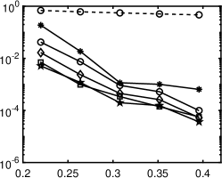
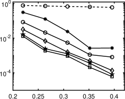
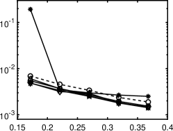
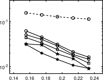
1 plots relative errors corresponding to the ratios of , showing that nonconvex regularizations (except for ) outperform the convex approach. In particular, the best regularizations for different polynomials are different, but - and ERF generally perform very well (within top two). TL1 works well in the cases of Legendre and Hermite polynomials, while is not numerically stable to guarantee satisfactory results. Please refer to Section 4.5 for in-depth discussions on the performance of these regularizations with respect to the matrix coherence.
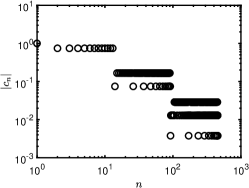
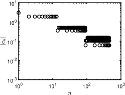
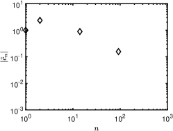
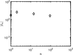
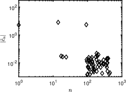
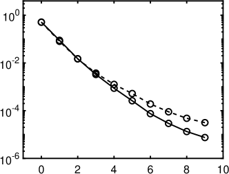
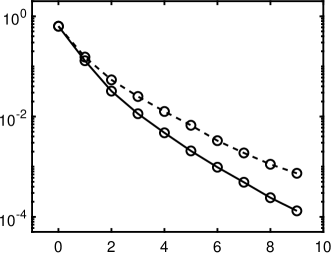
1 also indicates that the standard minimization without rotation is not effective, as its relative error is close to 50% even when approaches . Our iterative rotation methods with any regularization yield much higher accuracy, especially for a larger value. The reason can be partially explained by 2. Specifically, the plots (a), (b) and (c) of 2 are about the absolute values of exact coefficients of Legendre, Hermite, and Laguerre polynomials, while the plots (d), (e) and (f) show corresponding coefficients after 9 iterations with the - minimization using 120 samples randomly chosen from the independent experiments; we exclude whose absolute value is smaller than , since they are sufficiently small (more than two magnitudes smaller than the dominating ones). As demonstrated in Figure 2, the iterative updates on the rotation matrix significantly sparsifies the representation of ; and as a result, the efficiency of CS methods is substantially enhanced. Moreover, for the Laguerre polynomial is not as sparse as the ones for the Legendre and Hermite polynomials. Consequently, the Laguerre polynomial shows less accurate results in 1(c) compared with other two polynomials in 1(a) and (b). The phenomenon can be partially explained by the coherence of for different polynomials, i.e., the coherence in the Laguerre case is much larger ( before rotation and after rotation) than the other two, thus making any sparse regression algorithms less effective. For more detailed discussion on coherence, please refer to Table 5 and Section 4.5.

4.2 Elliptic Equation
Next we consider a one-dimensional elliptic differential equation with a random coefficient [20, 65]:
| (43) | ||||
where is a log-normal random field based on Karhunen-Loève (KL) expansion:
| (44) |
are i.i.d. random variables, and are eigenvalues/eigenfunctions (in a descending order in ) of an exponential covariance kernel:
| (45) |
The value of and the analytical expressions for are given in [31]. We set and such that . For each input sample , the solution of the deterministic elliptic equation can be obtained by [64]:
| (46) |
By imposing the boundary condition , we can compute as
| (47) |
The integrals in Eqs. (46) and (47) are obtained by highly accurate numerical integration. For this example, we choose the quantity of interest to be at . We aim to build a third-order Legendre (or Hermite) polynomial expansion which includes basis functions. The relative error is approximated by a level- sparse grid method. The parameters are given in 2.
| UQ setting | Legendre | Hermite | ||
|---|---|---|---|---|
| TL | ||||
| ERF | ||||
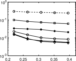
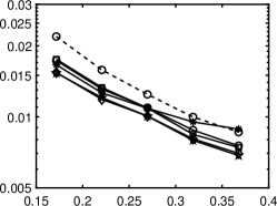
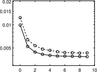
Relative errors of the Legendre and Hermite polynomial expansions are presented in 3. All the methods with rotation perform almost the same, except that yields unstable results, especially when sample size is small. In this case, we do not observe significant improvement of the nonconvex regularizations over the convex model, as opposed to 1. - and ERF perform the best for both Legendre and Hermite polynomials. In this case, the solution does not have an underlying low-dimensional structure under rotation as in the previous example and the truncation error exists, which is common in practical problems. This is why the improvement by the rotational method is minor.
4.3 Korteweg-de Vries equation
As an example of a more complicated and nonlinear differential equation, we consider the Korteweg-de Vries (KdV) equation with time-dependent additive noise,
| (48) |
Here is modeled as a random field represented by the Karhunen-Loève expansion:
| (49) |
where is a constant and are eigenvalues/eigenfunctions (in a descending order) of the exponential covariance kernel Eq. (45). We set and in (45) such that . Under this setting, we have an analytical solution given by
| (50) |
We choose QoI to be at and . Thanks to analytical expressions of , we can compute the integrals in (50) with high accuracy. Denote
| (51) |
the analytical solution can be written as
| (52) |
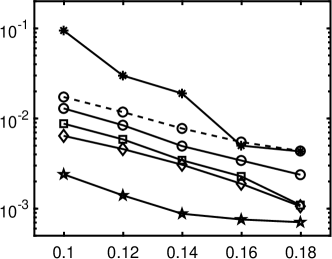
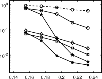
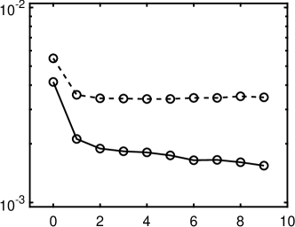
We use a fourth-order gPC expansion to approximate the solution, i.e., , and the number of gPC basis functions is . The experiment is repeated times to compute the average relative errors for each gPC expansion. Parameters chosen for different regularizations are given in 3. Relative errors of the Legendre and Hermite polynomial expansions are presented in 4, which illustrates the combined method of iterative rotation and nonconvex minimization outperforms the simple approaches. The coherence of for Legendre polynomial is around 0.6/0.85 before/after the rotation, while it becomes over 0.92 for the Hermite polynomial. In such highly coherent regime, does not work very well, and other nonconvex regularizations, i.e., ERF, TL1 and -, perform better than in the Hermite polynomial case, especially ERF.
| Method | Legendre | Hermite | ||
|---|---|---|---|---|
| Transformed | ||||
| ERF | ||||
4.4 High-dimensional function
We illustrate the potential capability of the proposed approach for dealing with higher-dimensional problems, referred to as HD function. Specifically, we select a function similar to the one in Section 4.1 but with a much higher dimension,
| (53) |
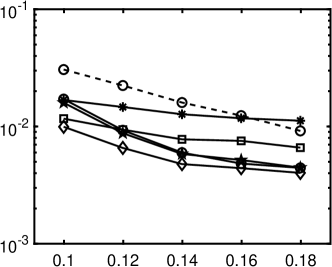
The total number of basis functions for this example is . The experiment is repeated times to compute the average relative errors for each polynomial. Parameters for this set of experiments are given in 4. The results are presented in 5, showing that all nonconvex methods with rotation outperforms the approach except for ERF under the Hermite basis when sample size is small. Different from previous examples (ridge, elliptic, and KdV), achieves the best result, as the corresponding coherence is relatively small, around 0.2/0.3 before/after rotation for the Legendre polynomial, and for the Hermite polynomial. In addition, 5 (b) suggests that ERF method is stable with respect to sampling ratios for the Hermite basis.
| UQ setting | Legendre | Hermite | ||
|---|---|---|---|---|
| TL1 | ||||
| ERF | ||||
4.5 Discussion
We intend to discuss the effects of coherence and the number of rotations on the performance of the and other nonconvex approaches. As reported in [26, 37, 70], - and ERF methods perform particularly well for coherent matrices (i.e., large ) and performs well for incoherenct matrices (i.e., small ), which motivates us to compute the coherence values and report in 5, 6 using the - method for ridge and elliptic/KdV/HD, respectively. Here, we use of each iteration by - as an examples, and its value for other regularizations (including ) are similar. Both tables confirm that applying rotation increases the coherence level of the sensing matrix except for the Hermite basis. As we show in numerical examples, when the coherence is large (e.g., around 0.9 or even larger in Hermite polynomial for KdV) - and ERF perform better than the convex method. When the coherence is small (e.g., in the high-dimensional case) gives the best results among all the competing methods. One the other hand, may lead to unstable and unsatisfactory results, sometimes even worse than the convex method, when the coherence of the sensing matrix is large. In the extreme case when the coherence is close to (e.g., Laguerre in ridge function), the best result is only slightly better than , which seems difficult for any sparse recovery algorithms to succeed. This series of observations coincide with the empirical performance in CS, i.e., works the best for incoherent matrices, while - and ERF work better for coherent cases.
| Ridge function | |||
|---|---|---|---|
| Rotations | Legendre | Hermite | Laguerre |
| 0 | 0.4692 | 0.7622 | 0.9448 |
| 3 | 0.6833 | 0.7527 | 0.9910 |
| 6 | 0.6822 | 0.7519 | 0.9911 |
| 9 | 0.6762 | 0.7657 | 0.9911 |
| Elliptic equation | KdV equation | HD function | ||||
|---|---|---|---|---|---|---|
| Rotations | Legendre | Hermite | Legendre | Hermite | Legendre | Hermite |
| 0 | 0.5014 | 0.7770 | 0.6079 | 0.9121 | 0.2117 | 0.2852 |
| 1 | 0.6958 | 0.7830 | 0.8825 | 0.9223 | 0.2580 | 0.3075 |
| 2 | 0.6943 | 0.7719 | 0.8487 | 0.9167 | 0.2664 | 0.2956 |
| 3 | 0.6896 | 0.7710 | 0.8677 | 0.9214 | 0.2522 | 0.3003 |
We then examine the effect of the number of rotations in 6. Here we use ridge function and KdV equation as an examples, and show the results by -. For ridge function, more rotations lead to a better accuracy, while it stagnates at 3-5 rotations for the KdV equation. This is because the ridge function has very good low-dimensional structure, i.e., the dimension can be reduced to one using a linear transformation , while the KdV equation does not have this property. Also, there is no truncation error when using the gPC expansion to represent the ridge function as we use a third order expansion, while exists for the KdV equation. In most practical problems, the truncation error exists and the linear transform may not yield the optimal low-dimensional structure to have sparse coefficients of the gPC expansion. Therefore, we empirically set a maximum number of rotations to terminate iterations in the algorithm.
Finally, we present the computation time in 7. All the experiments are performed on an AMD Ryzen 5 3600, 16 GB RAM machine on Windows 10 1904 and 2004 with MATLAB 2018b. The major computation comes from two components: one is the - minimization and the other is to find the rotation matrix . The computation complexity for every iteration of the - algorithm is which reduces to as we assume In practice, we choose the maximum outer/inner numbers in Algorithm 1 as respectively, and hence the complexity for - algorithm is . To find the rotation matrix one has to construct a matrix using (33) with complexity of followed by SVD with complexity of Therefore, the total complexity of our approach is per rotation. We divide the time of Legendre polynomial reported in 7 by getting , and As the ratios are of the same order, the empirical results are consistent with the complexity analysis.
| Time (sec.) | dimension | rotations | Legendre | Hermite | Laguerre |
|---|---|---|---|---|---|
| Ridge function | 9 | 6.53 | 4.31 | 16.19 | |
| Elliptic equation | 3 | 5.26 | 11.96 | N/A | |
| KdV equation | 3 | 15.03 | 14.33 | N/A | |
| HD function | 3 | 2041.82 | 2102.04 | N/A |
5 Conclusions
In this work, we proposed an alternating direction method to identify a rotation matrix iteratively in order to enhance the sparsity of gPC expansion, followed by several nonconvex minimization scheme to efficiently identify the sparse coefficients. We used a general framework to incorporate any regularization whose proximal operator can be found efficiently (including ) into the rotational method. As such, it improves the accuracy of the compressive sensing method to construct the gPC expansions from a small amount of data. In particular, the rotation is determined by seeking the directions of maximum variation for the QoI through SVD of the gradients at different points in the parameter space. The linear system after rotations becomes ill-conditioned, specifically more coherent, which motivated us to choose the nonconvex method instead of the convex approach for sparse recovery. We conducted extensive simulations under various scenarios, including a ridge function, an elliptic equation, KdV equation, and a HD function with Legendre, Hermite, and Laguerre polynomials, all of which are widely used in practice. Our experimental results demonstrated that the proposed combination of rotation estimation and nonconvex methods significantly outperforms the standard minimization (without rotation). In different coherence scenarios, there are different nonconvex regularizations (combined with rotations) that outperforms the rotational CS with the approach. Specifically, - and ERF work well for coherent systems, while excels in incoherent ones, which are aligned with the observations in CS studies.
Acknowledgement
This work was partially supported by NSF CAREER 1846690. Xiu Yang was supported by the U.S. Department of Energy (DOE), Office of Science, Office of Advanced Scientific Computing Research (ASCR) as part of Multifaceted Mathematics for Rare, Extreme Events in Complex Energy and Environment Systems (MACSER).
References
- [1] B. Adcock, Infinite-dimensional compressed sensing and function interpolation, Found. of Comput. Math., (2017), pp. 1–41.
- [2] B. Adcock, S. Brugiapaglia, and C. G. Webster, Compressed sensing approaches for polynomial approximation of high-dimensional functions, in Compressed Sensing and its Applications, Springer, 2017, pp. 93–124.
- [3] N. Alemazkoor and H. Meidani, Divide and conquer: An incremental sparsity promoting compressive sampling approach for polynomial chaos expansions, Comput. Methods Appl. Mech. Eng., 318 (2017), pp. 937–956.
- [4] I. Babuška, F. Nobile, and R. Tempone, A stochastic collocation method for elliptic partial differential equations with random input data, SIAM Rev., 52 (2010), pp. 317–355.
- [5] A. S. Bandeira, E. Dobriban, D. G. Mixon, and W. F. Sawin, Certifying the restricted isometry property is hard, IEEE Trans. Inf. Theory, 59 (2013), pp. 3448–3450.
- [6] G. Blatman and B. Sudret, Adaptive sparse polynomial chaos expansion based on least angle regression, J. Comput. Phys., 230 (2011), pp. 2345–2367.
- [7] S. Boyd, N. Parikh, E. Chu, B. Peleato, and J. Eckstein, Distributed optimization and statistical learning via the alternating direction method of multipliers, Found. Trends Mach. Learn., 3 (2011), pp. 1–122.
- [8] A. M. Bruckstein, D. L. Donoho, and M. Elad, From sparse solutions of systems of equations to sparse modeling of signals and images, SIAM Rev., 51 (2009), pp. 34–81.
- [9] R. H. Cameron and W. T. Martin, The orthogonal development of non-linear functionals in series of fourier-hermite functionals, Ann. Math., (1947), pp. 385–392.
- [10] E. J. Candès, The restricted isometry property and its implications for compressed sensing, C.R. Math., 346 (2008), pp. 589–592.
- [11] E. J. Candès, J. K. Romberg, and T. Tao, Stable signal recovery from incomplete and inaccurate measurements, Comm. Pure Appl. Math, 59 (2006), pp. 1207–1223.
- [12] E. J. Candès and M. B. Wakin, An introduction to compressive sampling, IEEE Signal Process. Mag., 25 (2008), pp. 21–30.
- [13] E. J. Candès, M. B. Wakin, and S. P. Boyd, Enhancing sparsity by reweighted l1 minimization, J. Fourier Anal. Appl., 14 (2008), pp. 877–905.
- [14] R. Chartrand, Exact reconstruction of sparse signals via nonconvex minimization, IEEE Signal Process Lett., 14 (2007), pp. 707–710.
- [15] P. G. Constantine, E. Dow, and Q. Wang, Active subspace methods in theory and practice: Applications to kriging surfaces, SIAM J. Sci. Comput., 36 (2014), pp. A1500–A1524.
- [16] W. Dai and O. Milenkovic, Subspace pursuit for compressive sensing: Closing the gap between performance and complexity, tech. rep., ILLINOIS UNIV AT URBANA-CHAMAPAIGN, 2008.
- [17] D. L. Donoho, Compressed sensing, IEEE Trans. Inf. Theory, 52 (2006), pp. 1289–1306.
- [18] D. L. Donoho and M. Elad, Optimally sparse representation in general (nonorthogonl) dictionaries via l1 minimization, Proc. Nat. Acad. Scien. USA, 100 (2003), pp. 2197–2202.
- [19] D. L. Donoho, M. Elad, and V. N. Temlyakov, Stable recovery of sparse overcomplete representations in the presence of noise, IEEE Trans. Inf. Theory, 52 (2006), pp. 6–18.
- [20] A. Doostan and H. Owhadi, A non-adapted sparse approximation of PDEs with stochastic inputs, J. Comput. Phys., 230 (2011), pp. 3015–3034.
- [21] O. G. Ernst, A. Mugler, H.-J. Starkloff, and E. Ullmann, On the convergence of generalized polynomial chaos expansions, ESAIM: Math. Model. Numer. Anal., 46 (2012), pp. 317–339.
- [22] S. Foucart and H. Rauhut, A mathematical introduction to compressive sensing, Birkhäuser Basel, 2013.
- [23] R. G. Ghanem and P. D. Spanos, Stochastic finite elements: a spectral approach, Springer-Verlag, New York, 1991.
- [24] R. Gribonval and M. Nielsen, Sparse representations in unions of bases, IEEE Trans. Inf. Theory, 49 (2003), pp. 3320–3325.
- [25] L. Guo, J. Li, and Y. Liu, Stochastic collocation methods via minimisation of the transformed -penalty, East Asian Journal on Applied Mathematics, 8 (2018), pp. 566–585.
- [26] W. Guo, Y. Lou, J. Qin, and M. Yan, A novel regularization based on the error function for sparse recovery, arXiv preprint arXiv:2007.02784, (2020).
- [27] J. Hampton and A. Doostan, Compressive sampling of polynomial chaos expansions: Convergence analysis and sampling strategies, J. Comput. Phys., 280 (2015), pp. 363–386.
- [28] , Basis adaptive sample efficient polynomial chaos (base-pc), J. Comput. Phys., 371 (2018), pp. 20–49.
- [29] J. D. Jakeman, M. S. Eldred, and K. Sargsyan, Enhancing -minimization estimates of polynomial chaos expansions using basis selection, J. Comput. Phys., 289 (2015), pp. 18–34.
- [30] J. D. Jakeman, A. Narayan, and T. Zhou, A generalized sampling and preconditioning scheme for sparse approximation of polynomial chaos expansions, SIAM J. Sci. Comput., 39 (2017), pp. A1114–A1144.
- [31] M. Jardak, C.-H. Su, and G. E. Karniadakis, Spectral polynomial chaos solutions of the stochastic advection equation, J. Sci. Comput., 17 (2002), pp. 319–338.
- [32] M.-J. Lai, Y. Xu, and W. Yin, Improved iteratively reweighted least squares for unconstrained smoothed minimization, SIAM J. Numer. Anal., 51 (2013), pp. 927–957.
- [33] H. Lei, X. Yang, Z. Li, and G. E. Karniadakis, Systematic parameter inference in stochastic mesoscopic modeling, J. Comput. Phys., 330 (2017), pp. 571–593.
- [34] H. Lei, X. Yang, B. Zheng, G. Lin, and N. A. Baker, Constructing surrogate models of complex systems with enhanced sparsity: quantifying the influence of conformational uncertainty in biomolecular solvation, SIAM Multiscale Model. Simul., 13 (2015), pp. 1327–1353.
- [35] K.-C. Li, Sliced inverse regression for dimension reduction, J. Am. Stat. Assoc., 86 (1991), pp. 316–327.
- [36] Y. Lou and M. Yan, Fast l1-l2 minimization via a proximal operator, J. Sci. Comput., 74 (2018), pp. 767–785.
- [37] Y. Lou, P. Yin, Q. He, and J. Xin, Computing sparse representation in a highly coherent dictionary based on difference of and , J. Sci. Comput., 64 (2015), pp. 178–196.
- [38] Y. Lou, P. Yin, and J. Xin, Point source super-resolution via non-convex l1 based methods, J. Sci. Comput., 68 (2016), pp. 1082–1100.
- [39] J. Lv, Y. Fan, et al., A unified approach to model selection and sparse recovery using regularized least squares, Annals of Stat., 37 (2009), pp. 3498–3528.
- [40] X. Ma and N. Zabaras, An adaptive high-dimensional stochastic model representation technique for the solution of stochastic partial differential equations, J. Comput. Phys., 229 (2010), pp. 3884–3915.
- [41] B. K. Natarajan, Sparse approximate solutions to linear systems, SIAM J. Comput., 24 (1995), pp. 227–234.
- [42] H. Ogura, Orthogonal functionals of the Poisson process, IEEE Trans. Inf. Theory, 18 (1972), pp. 473–481.
- [43] J. Peng, J. Hampton, and A. Doostan, A weighted -minimization approach for sparse polynomial chaos expansions, J. Comput. Phys., 267 (2014), pp. 92–111.
- [44] , On polynomial chaos expansion via gradient-enhanced -minimization, J. Comput. Phys., 310 (2016), pp. 440–458.
- [45] Y. Rahimi, C. Wang, H. Dong, and Y. Lou, A scale invariant approach for sparse signal recovery, SIAM J. Sci. Comput., 41 (2019), pp. A3649–A3672.
- [46] H. Rauhut and R. Ward, Sparse legendre expansions via -minimization, J. Approx. Theory, 164 (2012), pp. 517–533.
- [47] H. Rauhut and R. Ward, Interpolation via weighted minimization, Appl. Comput. Harmon. Anal., 40 (2016), pp. 321 – 351.
- [48] T. M. Russi, Uncertainty quantification with experimental data and complex system models, PhD thesis, UC Berkeley, 2010.
- [49] K. Sargsyan, C. Safta, H. N. Najm, B. J. Debusschere, D. Ricciuto, and P. Thornton, Dimensionality reduction for complex models via bayesian compressive sensing, Int. J. Uncertain. Quantif., 4 (2014).
- [50] X. Shen, W. Pan, and Y. Zhu, Likelihood-based selection and sharp parameter estimation, J. Am. Stat. Assoc., 107 (2012), pp. 223–232.
- [51] S. Smolyak, Quadrature and interpolation formulas for tensor products of certain classes of functions, Sov. Math. Dokl., 4 (1963), pp. 240–243.
- [52] M. A. Tatang, W. Pan, R. G. Prinn, and G. J. McRae, An efficient method for parametric uncertainty analysis of numerical geophysical models, J. Geophys. Res-Atmos. (1984–2012), 102 (1997), pp. 21925–21932.
- [53] A. M. Tillmann and M. E. Pfetsch, The computational complexity of the restricted isometry property, the nullspace property, and related concepts in compressed sensing, IEEE Trans. Inf. Theory, 60 (2014), pp. 1248–1259.
- [54] R. Tipireddy and R. Ghanem, Basis adaptation in homogeneous chaos spaces, J. Comput. Phys., 259 (2014), pp. 304–317.
- [55] P. Tsilifis, X. Huan, C. Safta, K. Sargsyan, G. Lacaze, J. C. Oefelein, H. N. Najm, and R. G. Ghanem, Compressive sensing adaptation for polynomial chaos expansions, J. Comput. Phys., 380 (2019), pp. 29–47.
- [56] C. Wang, M. Yan, Y. Rahimi, and Y. Lou, Accelerated schemes for the minimization, IEEE Trans. Signal Process., 68 (2020), pp. 2660–2669.
- [57] D. Xiu and J. S. Hesthaven, High-order collocation methods for differential equations with random inputs, SIAM J. Sci. Comput., 27 (2005), pp. 1118–1139.
- [58] D. Xiu and G. E. Karniadakis, The Wiener-Askey polynomial chaos for stochastic differential equations, SIAM J. Sci. Comput., 24 (2002), pp. 619–644.
- [59] Z. Xu, X. Chang, F. Xu, and H. Zhang, regularization: A thresholding representation theory and a fast solver, IEEE Trans. Neural Netw. Learn. Syst., 23 (2012), pp. 1013–1027.
- [60] Z. Xu and T. Zhou, On sparse interpolation and the design of deterministic interpolation points, SIAM J. Sci. Comput., 36 (2014), pp. A1752–A1769.
- [61] L. Yan, L. Guo, and D. Xiu, Stochastic collocation algorithms using -minimization, Int. J. Uncertain. Quan., 2 (2012), pp. 279–293.
- [62] X. Yang, D. A. Barajas-Solano, W. S. Rosenthal, and A. M. Tartakovsky, PDF estimation for power grid systems via sparse regression, arXiv preprint arXiv:1708.08378, (2017).
- [63] X. Yang, M. Choi, G. Lin, and G. E. Karniadakis, Adaptive ANOVA decomposition of stochastic incompressible and compressible flows, J. Comput. Phys., 231 (2012), pp. 1587–1614.
- [64] X. Yang and G. E. Karniadakis, Reweighted minimization method for stochastic elliptic differential equations, J. Comput. Phys., 248 (2013), pp. 87–108.
- [65] X. Yang, H. Lei, N. Baker, and G. Lin, Enhancing sparsity of Hermite polynomial expansions by iterative rotations, J. Comput. Phys., 307 (2016), pp. 94–109.
- [66] X. Yang, H. Lei, P. Gao, D. G. Thomas, D. L. Mobley, and N. A. Baker, Atomic radius and charge parameter uncertainty in biomolecular solvation energy calculations, J. Chem. Theory Comput., 14 (2018), pp. 759–767.
- [67] X. Yang, W. Li, and A. Tartakovsky, Sliced-inverse-regression–aided rotated compressive sensing method for uncertainty quantification, SIAM/ASA J. Uncertainty, 6 (2018), pp. 1532–1554.
- [68] X. Yang, X. Wan, L. Lin, and H. Lei, A general framework for enhancing sparsity of generalized polynomial chaos expansions, Int. J. Uncertain. Quantif., 9 (2019).
- [69] P. Yin, E. Esser, and J. Xin, Ratio and difference of and norms and sparse representation with coherent dictionaries, Comm. Inf. Syst., 14 (2014), pp. 87–109.
- [70] P. Yin, Y. Lou, Q. He, and J. Xin, Minimization of for compressed sensing, SIAM J. Sci. Comput., 37 (2015), pp. A536–A563.
- [71] S. Zhang and J. Xin, Minimization of transformed penalty: Closed form representation and iterative thresholding algorithms, Comm. Math. Sci., 15 (2017), pp. 511–537.
- [72] , Minimization of transformed penalty: theory, difference of convex function algorithm, and robust application in compressed sensing, Math. Program., 169 (2018), pp. 307–336.
- [73] T. Zhang, Multi-stage convex relaxation for learning with sparse regularization, in Adv. Neural Inf. Proces. Syst. (NIPS), 2009, pp. 1929–1936.
- [74] Z. Zhang, X. Yang, I. V. Oseledets, G. E. Karniadakis, and L. Daniel, Enabling high-dimensional hierarchical uncertainty quantification by ANOVA and tensor-train decomposition, IEEE Trans. Comput.-Aided Des. Integr. Circuits and Syst., 34 (2015), pp. 63–76.