This paper was converted on www.awesomepapers.org from LaTeX by an anonymous user.
Want to know more? Visit the Converter page.

A general Multidimensional Monte Carlo Approach for Dynamic Hedging under stochastic volatility

Dorival Leão Departamento de Matemática Aplicada e Estatística. Universidade de São Paulo, 13560-970, São Carlos - SP, Brazil leao@icmc.usp.br vinicns@icmc.usp.br Alberto Ohashi Departamento de Matemática, Universidade Federal da Paraíba, 13560-970, João Pessoa - Paraíba, Brazil alberto.ohashi@pq.cnpq.br  and  Vinícius Siqueira
(Date: August 12, 2025)
Abstract.

In this work, we introduce a Monte Carlo method for the dynamic hedging of general European-type contingent claims in a multidimensional Brownian arbitrage-free market. Based on bounded variation martingale approximations for Galtchouk-Kunita-Watanabe decompositions, we propose a feasible and constructive methodology which allows us to compute pure hedging strategies w.r.t arbitrary square-integrable claims in incomplete markets. In particular, the methodology can be applied to quadratic hedging-type strategies for fully path-dependent options with stochastic volatility and discontinuous payoffs. We illustrate the method with numerical examples based on generalized Föllmer-Schweizer decompositions, locally-risk minimizing and mean-variance hedging strategies for vanilla and path-dependent options written on local volatility and stochastic volatility models.

Key words and phrases:
Martingale representation, hedging contingent claims, path dependent options
1991 Mathematics Subject Classification:
Primary: C02; Secondary: G12
We would like to thank Bruno Dupire and Francesco Russo for stimulating discussions and several suggestions about the numerical algorithm proposed in this work. We also gratefully acknowledge the computational support from LNCC (Laboratório Nacional de Computação Científica - Brazil). The second author was supported by CNPq grant 308742.

1. Introduction

1.1. Background and Motivation

Let (S,𝐅,)(S,\mathbf{F},\mathbb{P}) be a financial market composed by a continuous 𝐅\mathbf{F}-semimartingale SS which represents a discounted risky asset price process, 𝐅={𝐅t;0tT}\mathbf{F}=\{\mathbf{F}_{t};0\leq t\leq T\} is a filtration which encodes the information flow in the market on a finite horizon [0,T][0,T], \mathbb{P} is a physical probability measure and e\mathcal{M}^{e} is the set of equivalent local martingale measures. Let HH be an 𝐅T\mathbf{F}_{T}-measurable contingent claim describing the net payoff whose the trader is faced at time TT. In order to hedge this claim, the trader has to choose a dynamic portfolio strategy.

Under the assumption of an arbitrage-free market, the classical Galtchouk-Kunita-Watanabe (henceforth abbreviated by GKW) decomposition yields

(1.1) H=𝔼[H]+0TθH,𝑑S+LTH,undere,H=\mathbb{E}_{\mathbb{Q}}[H]+\int_{0}^{T}\theta^{H,\mathbb{Q}}_{\ell}dS_{\ell}+L^{H,\mathbb{Q}}_{T}\quad\text{under}~\mathbb{Q}\in\mathcal{M}^{e},

where LH,L^{H,\mathbb{Q}} is a \mathbb{Q}-local martingale which is strongly orthogonal to SS and θH,\theta^{H,\mathbb{Q}} is an adapted process.

The GKW decomposition plays a crucial role in determining optimal hedging strategies in a general Brownian-based market model subject to stochastic volatility. For instance, if SS is a one-dimensional Itô risky asset price process which is adapted to the information generated by a two-dimensional Brownian motion W=(W1,W2)W=(W^{1},W^{2}), then there exists a two-dimensional adapted process ϕH,:=(ϕH,1,ϕH,2)\phi^{H,\mathbb{Q}}:=(\phi^{H,1},\phi^{H,2}) such that

H=𝔼[H]+0TϕtH,𝑑Wt,H=\mathbb{E}_{\mathbb{Q}}[H]+\int_{0}^{T}\phi^{H,\mathbb{Q}}_{t}dW_{t},

which also realizes

(1.2) θtH,=ϕtH,1[Stσt]1,LtH,=0tϕH,2𝑑Ws2;0tT.\theta^{H,\mathbb{Q}}_{t}=\phi^{H,1}_{t}[S_{t}\sigma_{t}]^{-1},\quad L^{H,\mathbb{Q}}_{t}=\int_{0}^{t}\phi^{H,2}dW^{2}_{s};~0\leq t\leq T.

In the complete market case, there exists a unique e\mathbb{Q}\in\mathcal{M}^{e} and in this case, LH,=0L^{H,\mathbb{Q}}=0, 𝔼[H]\mathbb{E}_{\mathbb{Q}}[H] is the unique fair price and the hedging replicating strategy is fully described by the process θH,\theta^{H,\mathbb{Q}}. In a general stochastic volatility framework, there are infinitely many GKW orthogonal decompositions parameterized by the set e\mathcal{M}^{e} and hence one can ask if it is possible to determine the notion of non-self-financing optimal hedging strategies solely based on the quantities (1.2). This type of question was firstly answered by Föllmer and Sonderman [9] and later on extended by Schweizer [23] and Föllmer and Schweizer [8] through the existence of the so-called Föllmer-Schweizer decomposition which turns out to be equivalent to the existence of locally-risk minimizing hedging strategies. The GKW decomposition under the so-called minimal martingale measure constitutes the starting point to get locally risk minimizing strategies provided one is able to check some square-integrability properties of the components in (1.1) under the physical measure. See e.g [12] and [26] for details and other references therein. Orthogonal decompositions without square-integrability properties can also be defined in terms of the the so-called generalized Föllmer-Schweizer decomposition (see e.g Schweizer [24]).

In contrast to the local-risk minimization approach, one can insist in working with self-financing hedging strategies which give rise to the so-called mean-variance hedging methodology. In this approach, the spirit is to minimize the expectation of the squared hedging error over all initial endowments xx and all suitable admissible strategies φΘ\varphi\in\Theta:

(1.3) infφΘ,x𝔼|Hx0Tφt𝑑St|2.\inf_{\varphi\in\Theta,x\in\mathbb{R}}\mathbb{E}_{\mathbb{P}}\Big{|}H-x-\int_{0}^{T}\varphi_{t}dS_{t}\Big{|}^{2}.

The nature of the optimization problem (1.3) suggests to work with the subset 2e:={e;ddL2()}\mathcal{M}^{e}_{2}:=\{\mathbb{Q}\in\mathcal{M}^{e};\frac{d\mathbb{Q}}{d\mathbb{P}}\in L^{2}(\mathbb{P})\}. Rheinlander and Schweizer [22], Gourieroux, Laurent and Pham [10] and Schweizer [25] show that if 2e\mathcal{M}^{e}_{2}\neq\emptyset and HL2()H\in L^{2}(\mathbb{P}) then the optimal quadratic hedging strategy exists and it is given by (𝔼~[H],η~)\big{(}\mathbb{E}_{\tilde{\mathbb{P}}}[H],\eta^{\tilde{\mathbb{P}}}\big{)}, where

(1.4) ηt~:=θtH,~ζ~tZ~t(VtH,~𝔼~[H]0tη~𝑑S);0tT.\eta^{\tilde{\mathbb{P}}}_{t}:=\theta^{H,\tilde{\mathbb{P}}}_{t}-\frac{\tilde{\zeta}_{t}}{\tilde{Z}_{t}}\Bigg{(}V^{H,\tilde{\mathbb{P}}}_{t-}-\mathbb{E}_{\tilde{\mathbb{P}}}[H]-\int_{0}^{t}\eta^{\tilde{\mathbb{P}}}_{\ell}dS_{\ell}\Bigg{)};~0\leq t\leq T.

Here θH,~\theta^{H,\tilde{\mathbb{P}}} is computed in terms of ~\tilde{\mathbb{P}}, the so-called variance optimal martingale measure, ζ~\tilde{\zeta} realizes

(1.5) Z~t:=𝔼~[d~d|𝐅t]=Z~0+0tζ~𝑑S;0tT,\tilde{Z}_{t}:=\mathbb{E}_{\tilde{\mathbb{P}}}\Bigg{[}\frac{d\tilde{\mathbb{P}}}{d\mathbb{P}}\Big{|}\mathbf{F}_{t}\Bigg{]}=\tilde{Z}_{0}+\int_{0}^{t}\tilde{\zeta}_{\ell}dS_{\ell};~0\leq t\leq T,

and VH,~:=𝔼~[H|𝐅]V^{H,\tilde{\mathbb{P}}}:=\mathbb{E}_{\tilde{\mathbb{P}}}[H|\mathbf{F}_{\cdot}] is the value option price process under ~\tilde{\mathbb{P}}. See also Cerný and Kallsen [4] for the general semimartingale case and the works [16][18] and [19] for other utility-based hedging strategies based on GKW decompositions.

Concrete representations for the pure hedging strategies {θH,;=^,~}\{\theta^{H,\mathbb{Q}};\mathbb{Q}=\hat{\mathbb{P}},\tilde{\mathbb{P}}\} can in principle be obtained by computing cross-quadratic variations d[VH,,S]t/d[S,S]td[V^{H,\mathbb{Q}},S]_{t}/d[S,S]_{t} for {~,^}\mathbb{Q}\in\{\tilde{\mathbb{P}},\hat{\mathbb{P}}\}. For instance, in the classical vanilla case, pure hedging strategies can be computed by means of the Feynman-Kac theorem (see e.g Heath, Platen and Schweizer [12]). In the path-dependent case, the obtention of concrete computationally efficient representations for θH,\theta^{H,\mathbb{Q}} is a rather difficult problem. Feynman-Kac-type arguments for fully path-dependent options mixed with stochastic volatility typically face not-well posed problems on the whole trading period as well as highly degenerate PDEs arise in this context. Generically speaking, one has to work with non-Markovian versions of the Feynman-Kac theorem in order to get robust dynamic hedging strategies for fully path dependent options written on stochastic volatility risky asset price processes.

In the mean variance case, the only quantity in (1.4) not related to GKW decomposition is Z~\tilde{Z} which can in principle be expressed in terms of the so-called fundamental representation equations given by Hobson [14] and Biagini, Guasoni and Pratelli [2] in the stochastic volatility case. For instance, Hobson derives closed form expressions for ζ~\tilde{\zeta} and also for any type of qq-optimal measure in the Heston model [13]. Recently, semi-explicit formulas for vanilla options based on general characterizations of the variance-optimal hedge in Cerný and Kallsen [4] have been also proposed in the literature which allow for a feasible numerical implementation in affine models. See Kallsen and Vierthauer [17] and Cerný and Kallsen [5] for some results in this direction. A different approach based on backward stochastic differential equations can also be used in order to get useful characterizations for the optimal mean variance hedging strategies. See e.g Jeanblanc, Mania, Santacrose and Schweizer [15] and other references therein.

1.2. Contribution of the current paper.

In spite of deep characterizations of optimal quadratic hedging strategies and concrete numerical schemes available for vanilla-type options, to our best knowledge no feasible approach has been proposed to tackle the problem of obtaining dynamic optimal quadratic hedging strategies for fully path dependent options written on a generic multidimensional Itô risky asset price process. In this work, we attempt to solve this problem with a probabilistic approach. The main difficulty in dealing with fully path dependent and/or discontinuous payoffs is the non-Markovian nature of the option value and a priori lack of path smoothness of the pure hedging strategies. Usual numerical schemes based on PDE and martingale techniques do not trivially apply to this context.

The main contribution of this paper is the obtention of flexible and computationally efficient multidimensional non-Markovian representations for generic option price processes which allow for a concrete computation of the associated GKW decomposition (θH,,LH,)\big{(}\theta^{H,\mathbb{Q}},L^{H,\mathbb{Q}}\big{)} for \mathbb{Q}-square integrable payoffs HH with e\mathbb{Q}\in\mathcal{M}^{e}. We provide a Monte Carlo methodology capable to compute optimal quadratic hedging strategies w.r.t general square-integrable claims in a multidimensional Brownian-based market model.

This article provides a feasible and constructive method to compute generalized Föllmer-Schweizer decompositions under full generality. As far as the mean variance hedging is concerned, we are able to compute pure optimal hedging strategies θH,~\theta^{H,\tilde{\mathbb{P}}} for arbitrary square-integrable payoffs. Hence, our methodology also applies to this case provided one is able to compute the fundamental representation equations in Hobson [14] and Biagini, Guasoni and Pratelli [2] which is the case for the classical Heston model. In mathematical terms, we are able to compute \mathbb{Q}-GKW decompositions under full generality so that the results of this article can also be used to other non-quadratic hedging methodologies where orthogonal martingale representations play an important role in determining optimal hedging strategies.

The starting point of this article is based on weak approximations developed by Leão and Ohashi [20] for one-dimensional Brownian functionals. They introduced a one-dimensional space-filtration discretization scheme constructed from suitable waiting times which measure the instants when the Brownian motion hits some a priori levels. In this work, we extend [20] to the multidimensional case as follows: More general and stronger convergence results are obtained in order to recover incomplete markets with stochastic volatility. Hitting times induced by multidimensional noises which drive the stochastic volatility are carefully analyzed in order to obtain \mathbb{Q}-GKW decompositions under rather weak integrability conditions for any e\mathbb{Q}\in\mathcal{M}^{e}. Moreover, a complete analysis is performed w.r.t weak approximations for gain processes by means of suitable non-antecipative discrete-time hedging strategies for square-integrable payoffs, including path-dependent ones.

It is important to stress that the results of this article can be applied to both complete and incomplete markets written on a generic multidimensional Itô risky asset price process. One important restriction of our methodology is the assumption that the risky asset price process has continuous paths. This is a limitation that we hope to overcome in a future work.

Numerical results based on the standard Black-Scholes, local-volatility and Heston models are performed in order to illustrate the theoretical results and the methodology of this article. In particular, we briefly compare our results with other prominent methodologies based on Malliavin weights (complete market case) and PDE techniques (incomplete market case) employed by Bernis, Gobet and Kohatsu-Higa [1] and Heath, Platen and Schweizer [12], respectively. The numerical experiments suggest that pure hedging strategies based on generalized Föllmer-Schweizer decompositions mitigate very well the cost of hedging of a path-dependent option even if there is no guarantee of the existence of locally-risk minimizing strategies. We also compare hedging errors arising from optimal mean variance hedging strategies for one-touch options written on a Heston model with nonzero correlation.

The remainder of this paper is structured as follows. In Section 2, we fix the notation and we describe the basic underlying market model. In Section 3, we provide the basic elements of the Monte Carlo methodology proposed in this article. In Section 4, we formulate dynamic hedging strategies starting from a given GKW decomposition and we translate our results to well-known quadratic hedging strategies. The Monte Carlo algorithm and the numerical study are described in Sections 5 and 6, respectively. The Appendix presents more refined approximations when the martingale representations admit additional hypotheses.

2. Preliminaries

Throughout this paper, we assume that we are in the usual Brownian market model with finite time horizon 0T<0\leq T<\infty equipped with the stochastic basis (Ω,𝐅,)(\Omega,\mathbf{F},\mathbb{P}) generated by a standard pp-dimensional Brownian motion B={(Bt(1),,Bt(p));0tT}B=\{(B^{(1)}_{t},\ldots,B^{(p)}_{t});0\leq t\leq T\} starting from 0. The filtration 𝐅:=(𝐅t)0tT\mathbf{F}:=(\mathbf{F}_{t})_{0\leq t\leq T} is the \mathbb{P}-augmentation of the natural filtration generated by BB. For a given mm-dimensional vector J=(J1,,Jm)J=(J_{1},\ldots,J_{m}), we denote by diag(J)\operatorname{diag}(J) the m×mm\times m diagonal matrix whose \ell-th diagonal term is JJ_{\ell}. In this paper, for all unexplained terminology concerning general theory of processes, we refer to Dellacherie and Meyer [6].

In view of stochastic volatility models, let us split BB into two multidimensional Brownian motions as follows BS:=(B(1),,B(d))B^{S}:=(B^{(1)},\ldots,B^{(d)}) and BI:=(B(d+1),,B(p))B^{I}:=(B^{(d+1)},\ldots,B^{(p)}). In this section, the market consists of d+1d+1 assets (dp)(d\leq p): one riskless asset given by

dSt0=rtSt0dt,S00=1;0tT,dS^{0}_{t}=r_{t}S^{0}_{t}dt,\quad S^{0}_{0}=1;\quad 0\leq t\leq T,

and a dd-dimensional vector of risky assets S¯:=(S¯1,,S¯d)\bar{S}:=(\bar{S}^{1},\ldots,\bar{S}^{d}) which satisfies the following stochastic differential equation

dS¯t=diag(S¯t)(btdt+σtdBtS),S¯0=x¯d;0tT.d\bar{S}_{t}=\operatorname{diag}(\bar{S}_{t})\left(b_{t}dt+\sigma_{t}dB^{S}_{t}\right),\quad\bar{S}_{0}=\bar{x}\in\mathbb{R}^{d};\quad 0\leq t\leq T.

Here, the real-valued interest rate process r={rt;0tT}r=\{r_{t};0\leq t\leq T\}, the vector of mean rates of return b:={bt=(bt1,,btd);0tT}b:=\{b_{t}=(b^{1}_{t},\ldots,b^{d}_{t});0\leq t\leq T\} and the volatility matrix σ:={σt=(σtij);1id,1jd,0tT}\sigma:=\{\sigma_{t}=(\sigma^{ij}_{t});1\leq i\leq d,1\leq j\leq d,~0\leq t\leq T\} are assumed to be predictable and they satisfy the standard assumptions in such way that both S0S^{0} and S¯\bar{S} are well-defined positive semimartingales. We also assume that the volatility matrix σ\sigma is non-singular for almost all (t,ω)[0,T]×Ω(t,\omega)\in[0,T]\times\Omega. The discounted price S:={Si:=S¯i/S0;i=1,,d}S:=\{S_{i}:=\bar{S}^{i}/S^{0};i=1,\ldots,d\} follows

dSt=diag(St)[(btrt1d)dt+σtdBtS];S0=xd,0tT,dS_{t}=\operatorname{diag}(S_{t})\left[(b_{t}-r_{t}\textbf{1}_{d})dt+\sigma_{t}dB^{S}_{t}\right];\quad S_{0}=x\in\mathbb{R}^{d},~0\leq t\leq T,

where 1d\textbf{1}_{d} is a d-dimensional vector with every component equal to 11. The market price of risk is given by

ψt:=σt1[btrt1d],0tT,\psi_{t}:=\sigma^{-1}_{t}\left[b_{t}-r_{t}\textbf{1}_{d}\right],\quad 0\leq t\leq T,

where we assume

0Tψud2𝑑u<a.s.\int_{0}^{T}\|\psi_{u}\|_{\mathbb{R}^{d}}^{2}du<\infty~a.s.

In the sequel, e\mathcal{M}^{e} denotes the set of \mathbb{P}-equivalent probability measures \mathbb{Q} such that the respective Radon-Nikodym derivative process is a \mathbb{P}-martingale and the discounted price SS is a \mathbb{Q}-local martingale. Throughout this paper, we assume that e\mathcal{M}^{e}\neq\emptyset. In our setup, it is well known that e\mathcal{M}^{e} is given by the subset of probability measures with Radon-Nikodym derivatives of the form

dd:=exp[0Tψu𝑑BuS0Tνu𝑑BuI120T{ψud2+νupd2}𝑑u],\frac{d\mathbb{Q}}{d\mathbb{P}}:=\exp\left[-\int_{0}^{T}\psi_{u}dB^{S}_{u}-\int_{0}^{T}\nu_{u}dB^{I}_{u}-\frac{1}{2}\int_{0}^{T}\big{\{}\|\psi_{u}\|^{2}_{\mathbb{R}^{d}}+\|\nu_{u}\|^{2}_{\mathbb{R}^{p-d}}\big{\}}du\right],

for some pd\mathbb{R}^{p-d}-valued adapted process ν\nu such that 0Tνtpd2𝑑t<\int_{0}^{T}\|\nu_{t}\|^{2}_{\mathbb{R}^{p-d}}dt<\infty a.s.

Example: The typical example studied in the literature is the following one-dimensional stochastic volatility model

(2.1) {dSt=Stμ(t,St,σt)dt+StσtdYt(1)dσt2=a(t,St,σt)dt+b(t,St,σt)dYt(2);0tT,\left\{\begin{array}[]{l}\displaystyle dS_{t}=S_{t}\mu(t,S_{t},\sigma_{t})dt+S_{t}\sigma_{t}dY_{t}^{(1)}\\ \displaystyle d\sigma_{t}^{2}=a(t,S_{t},\sigma_{t})dt+b(t,S_{t},\sigma_{t})dY^{(2)}_{t};~0\leq t\leq T,\end{array}\right.

where Y(1)Y^{(1)} and Y(2)Y^{(2)} are correlated Brownian motions with correlation ρ[1,1]\rho\in[-1,1], μ,a\mu,a and bb are suitable functions such that (S,σ2)(S,\sigma^{2}) is a well-defined two-dimensional Markov process. All continuous stochastic volatility model commonly used in practice fit into the specification (2.1). In this case, p=2>d=1p=2>d=1 and we recall that the market is incomplete where the set e\mathcal{M}^{e} is infinity. The dynamic hedging procedure turns out to be quite challenging due to extrinsic randomness generated by the non-tradeable volatility, specially w.r.t to exotic options.

2.1. GKW Decomposition

In the sequel, we take e\mathbb{Q}\in\mathcal{M}^{e} and we set WS:=(W(1),,W(d))W^{S}:=(W^{(1)},\ldots,W^{(d)}) and WI:=(W(d+1),,W(p))W^{I}:=(W^{(d+1)},\ldots,W^{(p)}) where

(2.2) Wt(j):={Bt(j)+0tψuj𝑑u,j=1,,dBt(j)+0tνuj𝑑u,j=d+1,,p;0tT,W^{(j)}_{t}:=\left\{\begin{array}[]{ll}\displaystyle B^{(j)}_{t}+\int_{0}^{t}\psi^{j}_{u}du,&j=1,\ldots,d\\ \displaystyle B^{(j)}_{t}+\int_{0}^{t}\nu^{j}_{u}du,&j=d+1,\ldots,p;~0\leq t\leq T,\end{array}\right.

is a standard pp-dimensional Brownian motion under the measure \mathbb{Q} and filtration 𝔽:={t;0tT}\mathbb{F}:=\{\mathcal{F}_{t};0\leq t\leq T\} generated by W=(W(1),,W(p))W=(W^{(1)},\ldots,W^{(p)}). In what follows, we fix a discounted contingent claim HH. Recall that the filtration 𝔽\mathbb{F} is contained in 𝐅\mathbf{F}, but it is not necessarily equal. In the remainder of this article, we assume the following hypothesis.

(M) The contingent claim HH is also T\mathcal{F}_{T}-measurable.

Remark 2.1.

Assumption (M) is essential for the approach taken in this work because the whole algorithm is based on the information generated by the Brownian motion WW (defined under the measure \mathbb{Q} and filtration 𝔽\mathbb{F}). As long as the numeraire is deterministic, this hypothesis is satisfied for any stochastic volatility model of the form (2.1) and a payoff Φ(St;0tT)\Phi(S_{t};0\leq t\leq T) where Φ:𝒞T\Phi:\mathcal{C}_{T}\rightarrow\mathbb{R} is a Borel map and 𝒞T\mathcal{C}_{T} is the usual space of continuous paths on [0,T][0,T]. Hence, (M) holds for a very large class of examples founded in practice.

For a given \mathbb{Q}-square integrable claim HH, the Brownian martingale representation (computed in terms of (𝔽,)(\mathbb{F},\mathbb{Q})) yields

H=𝔼[H]+0TϕuH,𝑑Wu,H=\mathbb{E}_{{\mathbb{Q}}}[H]+\int_{0}^{T}\phi^{H,\mathbb{Q}}_{u}dW_{u},

where ϕH,:=(ϕH,,1,,ϕH,,p)\phi^{H,\mathbb{Q}}:=(\phi^{H,\mathbb{Q},1},\ldots,\phi^{H,\mathbb{Q},p}) is a pp-dimensional 𝔽\mathbb{F}-predictable process. In what follows, we set ϕH,,S:=(ϕH,,1,,ϕH,,d)\phi^{H,\mathbb{Q},S}:=(\phi^{H,\mathbb{Q},1},\ldots,\phi^{H,\mathbb{Q},d}), ϕH,,I:=(ϕH,,d+1,,ϕH,,p)\phi^{H,\mathbb{Q},I}:=(\phi^{H,\mathbb{Q},d+1},\ldots,\phi^{H,\mathbb{Q},p}) and

(2.3) LtH,:=0tϕuH,,I𝑑WuI,V^t:=𝔼[H|t];0tT.L^{H,\mathbb{Q}}_{t}:=\int_{0}^{t}\phi^{H,\mathbb{Q},I}_{u}dW^{I}_{u},\quad\hat{V}_{t}:=\mathbb{E}_{\mathbb{Q}}[H|\mathcal{F}_{t}];~0\leq t\leq T.

The discounted stock price process has the following \mathbb{Q}-dynamics

dSt=diag(St)σtdWtS,S0=x,0tT,dS_{t}=\operatorname{diag}(S_{t})\sigma_{t}dW^{S}_{t},\quad S_{0}=x,~0\leq t\leq T,

and therefore the \mathbb{Q}-GKW decomposition for the pair of locally square integrable local martingales (V^,S)(\hat{V},S) is given by

V^t\displaystyle\hat{V}_{t} =𝔼[H]+0tϕuH,,S𝑑WuS+LtH,\displaystyle=\mathbb{E}_{\mathbb{Q}}[H]+\int_{0}^{t}\phi^{H,\mathbb{Q},S}_{u}dW^{S}_{u}+L^{H,\mathbb{Q}}_{t}
(2.4) =𝔼[H]+0tθuH,𝑑Su+LtH,;0tT,\displaystyle=\mathbb{E}_{\mathbb{Q}}[H]+\int_{0}^{t}\theta^{H,\mathbb{Q}}_{u}dS_{u}+L^{H,\mathbb{Q}}_{t};\quad 0\leq t\leq T,

where

(2.5) θH,:=ϕH,,S[diag(S)σ]1.\theta^{H,\mathbb{Q}}:=\phi^{H,\mathbb{Q},S}\left[\operatorname{diag}(S)\sigma\right]^{-1}.

The pp-dimensional process ϕH,\phi^{H,\mathbb{Q}} which constitutes (2.3) and (2.5) plays a major role in several types of hedging strategies in incomplete markets and it will be our main object of study.

Remark 2.2.

If we set νj=0\nu^{j}=0 for j=d+1,,pj=d+1,\ldots,p and the correspondent density process is a martingale then the resulting minimal martingale measure ^\hat{\mathbb{P}} yields a GKW decomposition where LH,^L^{H,\hat{\mathbb{P}}} is still a \mathbb{P}-local martingale orthogonal to the martingale component of SS under \mathbb{P}. In this case, it is also natural to implement a pure hedging strategy based on θH,^\theta^{H,\hat{\mathbb{P}}} regardless the existence of the Föllmer-Schweizer decomposition. If this is the case, this hedging strategy can be based on the generalized Föllmer-Schweizer decomposition (see e.g Th.9 in [24]).

3. The Random Skeleton and Weak Approximations for GKW Decompositions

In this section, we provide the fundamentals of the numerical algorithm of this article for the obtention of hedging strategies in complete and incomplete markets.

3.1. The Multidimensional Random Skeleton

At first, we fix once and for all e\mathbb{Q}\in\mathcal{M}^{e} and a \mathbb{Q}-square-integrable contingent claim HH satisfying (M). In the remainder of this section, we are going to fix a \mathbb{Q}-Brownian motion WW and with a slight abuse of notation all \mathbb{Q}-expectations will be denoted by 𝔼\mathbb{E}. The choice of e\mathbb{Q}\in\mathcal{M}^{e} is dictated by the pricing and hedging method used by the trader.

In the sequel, [,][\cdot,\cdot] denotes the usual quadratic variation between semimartingales and the usual jump of a process is denoted by ΔYt=YtYt\Delta Y_{t}=Y_{t}-Y_{t-} where YtY_{t-} is the left-hand limit of a cadlag process YY. For a pair (a,b)2(a,b)\in\mathbb{R}^{2}, we denote ab:=max{a,b}a\vee b:=\max\{a,b\} and ab:=min{a,b}a\wedge b:=\min\{a,b\}. Moreover, for any two stopping times SS and JJ, we denote the stochastic intervals [[S,J[[:={(ω,t);S(ω)t<J(ω)}[[S,J[[:=\{(\omega,t);S(\omega)\leq t<J(\omega)\}, [[S]]:={(ω,t);S(ω)=t}[[S]]:=\{(\omega,t);S(\omega)=t\} and so on. Throughout this article, LebLeb denotes the Lebesgue measure on the interval [0,T][0,T].

For a fixed positive integer kk and for each j=1,2,,pj=1,2,\ldots,p we define T0k,j:=0T^{k,j}_{0}:=0 a.s. and

(3.1) Tnk,j:=inf{Tn1k,j<t<;|Wt(j)WTn1k,j(j)|=2k},n1,T^{k,j}_{n}:=\inf\{T^{k,j}_{n-1}<t<\infty;|W^{(j)}_{t}-W^{(j)}_{T^{k,j}_{n-1}}|=2^{-k}\},\quad n\geq 1,

where W:=(W(1),,W(p))W:=(W^{(1)},\ldots,W^{(p)}) is the pp-dimensional \mathbb{Q}-Brownian motion as defined in (2.2).

For each j{1,,p}j\in\{1,\ldots,p\}, the family (Tnk,j)n0(T^{k,j}_{n})_{n\geq 0} is a sequence of 𝔽\mathbb{F}-stopping times where the increments {Tnk,jTn1k,j;n1}\{T^{k,j}_{n}-T^{k,j}_{n-1};n\geq 1\} is an i.i.d sequence with the same distribution as T1k,jT^{k,j}_{1}. In the sequel, we define Ak:=(Ak,1,,Ak,p)A^{k}:=(A^{k,1},\ldots,A^{k,p}) as the pp-dimensional step process given componentwise by

Atk,j:=n=12kηnk,j11{Tnk,jt};0tT,A^{k,j}_{t}:=\sum_{n=1}^{\infty}2^{-k}\eta^{k,j}_{n}1\!\!1_{\{T^{k,j}_{n}\leq t\}};~0\leq t\leq T,

where

(3.2) ηnk,j:={1;ifWTnk,j(j)WTn1k,j(j)=2kandTnk,j<1;ifWTnk,j(j)WTn1k,j(j)=2kandTnk,j<0;ifTnk,j=.\eta^{k,j}_{n}:=\left\{\begin{array}[]{rl}1;&\hbox{if}\ W^{(j)}_{T^{k,j}_{n}}-W^{(j)}_{T^{k,j}_{n-1}}=2^{-k}~~\mbox{and}~~T^{k,j}_{n}<\infty\\ -1;&\hbox{if}\ W^{(j)}_{T^{k,j}_{n}}-W^{(j)}_{T^{k,j}_{n-1}}=-2^{-k}~~\mbox{and}~~T^{k,j}_{n}<\infty\\ 0;&\hbox{if}\ T^{k,j}_{n}=\infty.\end{array}\right.

for k,n1k,n\geq 1 and j=1,,pj=1,\ldots,p. We split AkA^{k} into (AS,k,AI,k)(A^{S,k},A^{I,k}) where AS,kA^{S,k} is the dd-dimensional process constituted by the first dd components of AkA^{k} and AI,kA^{I,k} the remainder pdp-d-dimensional process. Let 𝔽k,j:={tk,j:0tT}\mathbb{F}^{k,j}:=\{\mathcal{F}^{k,j}_{t}:0\leq t\leq T\} be the natural filtration generated by {Atk,j;0tT}\{A^{k,j}_{t};0\leq t\leq T\}. One should notice that 𝔽k,j\mathbb{F}^{k,j} is a discrete-type filtration in the sense that

tk,j==0(Tk,jk,j{Tk,jt<T+1k,j}),0tT,\mathcal{F}^{k,j}_{t}=\bigvee_{\ell=0}^{\infty}\Big{(}\mathcal{F}^{k,j}_{T^{k,j}_{\ell}}\cap\{T^{k,j}_{\ell}\leq t<T^{k,j}_{\ell+1}\}\Big{)},~0\leq t\leq T,

where 0k,j={Ω,}\mathcal{F}^{k,j}_{0}=\{\Omega,\emptyset\} and Tmk,jk,j=σ(T1k,j,,Tmk,j,η1k,j,,ηmk,j)\mathcal{F}^{k,j}_{T^{k,j}_{m}}=\sigma(T^{k,j}_{1},\ldots,T^{k,j}_{m},\eta^{k,j}_{1},\ldots,\eta^{k,j}_{m}) for m1m\geq 1 and j=1,,pj=1,\ldots,p. Here, \bigvee denotes the smallest sigma-algebra generated by the union. One can easily check that Tmk,jk,j=σ(AsTmk,jk,j;s0)\mathcal{F}^{k,j}_{T^{k,j}_{m}}=\sigma(A^{k,j}_{s\wedge T^{k,j}_{m}};s\geq 0) and hence

Tmk,jk,j=tk,ja.son{Tmk,jt<Tm+1k,j}.\mathcal{F}^{k,j}_{T^{k,j}_{m}}=\mathcal{F}^{k,j}_{t}~a.s~\text{on}~\big{\{}T^{k,j}_{m}\leq t<T^{k,j}_{m+1}\big{\}}.

With a slight abuse of notation we write tk,j\mathcal{F}^{k,j}_{t} to denote its \mathbb{Q}-augmentation satisfying the usual conditions.

Let us now introduce the multidimensional filtration generated by AkA^{k}. Let us consider 𝔽k:={tk;0tT}\mathbb{F}^{k}:=\{\mathcal{F}^{k}_{t};0\leq t\leq T\} where tk:=tk,1tk,2tk,p\mathcal{F}^{k}_{t}:=\mathcal{F}^{k,1}_{t}\otimes\mathcal{F}^{k,2}_{t}\otimes\cdots\otimes\mathcal{F}^{k,p}_{t} for 0tT0\leq t\leq T. Let 𝒯k:={Tmk;m0}\mathcal{T}^{k}:=\{T^{k}_{m};m\geq 0\} be the order statistics obtained from the family of random variables {Tk,j;0;j=1,,p}\{T^{k,j}_{\ell};\ell\geq 0;j=1,\ldots,p\}. That is, we set T0k:=0T^{k}_{0}:=0,

(3.3) T1k:=inf1jpm1{Tmk,j},Tnk:=inf1jpm1{Tmk,j;Tmk,jT1kTn1k}T^{k}_{1}:=\inf_{\begin{subarray}{c}1\leq j\leq p\\ m\geq 1\end{subarray}}\Big{\{}T^{k,j}_{m}\Big{\}},\quad T^{k}_{n}:=\inf_{\begin{subarray}{c}1\leq j\leq p\\ m\geq 1\end{subarray}}\Big{\{}T^{k,j}_{m};T^{k,j}_{m}\geq T^{k}_{1}\vee\ldots\vee T^{k}_{n-1}\Big{\}}

for n1n\geq 1. In this case, 𝒯k\mathcal{T}^{k} is the partition generated by all stopping times defined in (3.1). The finite-dimensional distribution of W(j)W^{(j)} is absolutely continuous for each j=1,,pj=1,\ldots,p and therefore the elements of 𝒯k\mathcal{T}^{k} are almost surely distinct for every k1k\geq 1. Moreover, the following result holds true.

Lemma 3.1.

For every k1k\geq 1, the set 𝒯k\mathcal{T}^{k} is an exhaustive sequence of 𝔽k\mathbb{F}^{k}-stopping times such that supn1|TnkTn1k|0\sup_{n\geq 1}|T^{k}_{n}-T^{k}_{n-1}|\rightarrow 0 in probability as kk\rightarrow\infty.

Proof.

The following obvious estimate holds

supn1|TnkTn1k|max1jpsupn1|Tnk,jTn1k,j|0,\sup_{n\geq 1}|T^{k}_{n}-T^{k}_{n-1}|\leq\max_{1\leq j\leq p}\sup_{n\geq 1}|T^{k,j}_{n}-T^{k,j}_{n-1}|\rightarrow 0,

in probability as kk\rightarrow\infty and TnkT^{k}_{n}\rightarrow\infty a.s as nn\rightarrow\infty for each k1k\geq 1. Let us now prove that 𝒯k={Tnk;n0}\mathcal{T}^{k}=\{T^{k}_{n};n\geq 0\} is a sequence of 𝔽k\mathbb{F}^{k}-stopping times. In order to show this, we write (Tnk)n0(T^{k}_{n})_{n\geq 0} in a different way. This sequence can be defined recursively as follows

T0k=0,T1k=inf{t>0;Atkp=2k},T^{k}_{0}=0,\quad T^{k}_{1}=\inf\{t>0;\parallel A^{k}_{t}\parallel_{\mathbb{R}^{p}}=2^{-k}\},

where p\parallel\cdot\parallel_{\mathbb{R}^{p}} denotes the p\mathbb{R}^{p}-maximum norm. Therefore, T1kT^{k}_{1} is an 𝔽k\mathbb{F}^{k}-stopping time. Next, let us define a family of T1kk\mathcal{F}^{k}_{T^{k}_{1}}-random variables related to the index jj which realizes the hitting time T1kT^{k}_{1} as follows

1k,j:={0,ifAT1kk,j2k1,ifAT1kk,j=2k,\ell^{k,j}_{1}:=\left\{\begin{array}[]{l}0,\ \hbox{if}\ \mid A^{k,j}_{T^{k}_{1}}\mid\neq 2^{-k}\\ \\ 1,\ \hbox{if}\ \mid A^{k,j}_{T^{k}_{1}}\mid=2^{-k},\end{array}\right.

for any j=1,,pj=1,\ldots,p. Then, we shift AkA^{k} as follows

A~1k(t):=(A~1k,1(t):=Ak,1(t+T1k)Ak,1(T1k,1k);;A~1k,p(t):=Ak,p(t+T1k)Ak,p(T1k,pk)),\tilde{A}^{k}_{1}(t):=\left(\tilde{A}^{k,1}_{1}(t):=A^{k,1}(t+T^{k}_{1})-A^{k,1}(T^{k}_{\ell^{k,1}_{1}});\ldots;\tilde{A}^{k,p}_{1}(t):=A^{k,p}(t+T^{k}_{1})-A^{k,p}(T^{k}_{\ell^{k,p}_{1}})\right),

for t0t\geq 0. In this case, we conclude that A~1k\tilde{A}^{k}_{1} is adapted to the filtration {t+T1kk;t0}\{\mathcal{F}^{k}_{t+T^{k}_{1}};t\geq 0\}, the hitting time

S2k:=inf{t>0;A~1k(t)p=2k}S^{k}_{2}:=\inf\{t>0;\parallel\tilde{A}^{k}_{1}(t)\parallel_{\mathbb{R}^{p}}=2^{-k}\}

is a {t+T1kk:t0}\{\mathcal{F}^{k}_{t+T^{k}_{1}}:t\geq 0\}-stopping time and T2k=T1k+S2kT^{k}_{2}=T^{k}_{1}+S^{k}_{2} is a 𝔽k\mathbb{F}^{k}-stopping time. In the sequel, we define a family of T2kk\mathcal{F}^{k}_{T^{k}_{2}}-random variables related to the index jj which realizes the hitting time T2kT^{k}_{2} as follows

2k,j:={0,ifA~1k,j(S2k)2k2,ifA~1k,j(S2k)=2k,\ell^{k,j}_{2}:=\left\{\begin{array}[]{l}0,\ \hbox{if}\ \mid\tilde{A}^{k,j}_{1}(S^{k}_{2})\mid\neq 2^{-k}\\ 2,\ \hbox{if}\ \mid\tilde{A}^{k,j}_{1}(S^{k}_{2})\mid=2^{-k},\end{array}\right.

for j=1,,pj=1,\ldots,p. If we denote S0k=0S^{k}_{0}=0, we shift A~1k\tilde{A}^{k}_{1} as follows

A~2k(t):=(A~2k,1(t):=A~1k,1(t+S2k)A~1k,1(S2k,1k);;A~2k,p(t)=A~k,p(t+S2k)A~k,p(S2k,pk)),\tilde{A}^{k}_{2}(t):=\left(\tilde{A}^{k,1}_{2}(t):=\tilde{A}^{k,1}_{1}(t+S^{k}_{2})-\tilde{A}^{k,1}_{1}(S^{k}_{\ell^{k,1}_{2}});\ldots;\tilde{A}^{k,p}_{2}(t)=\tilde{A}^{k,p}(t+S^{k}_{2})-\tilde{A}^{k,p}(S^{k}_{\ell^{k,p}_{2}})\right),

for every t0t\geq 0. In this case, we conclude that A~2k\tilde{A}^{k}_{2} is adapted to the filtration {t+T2kk;t0}\{\mathcal{F}^{k}_{t+T^{k}_{2}};t\geq 0\}, the hitting time

S3k=inf{t>0;A~2k(t)p=2k}S^{k}_{3}=\inf\{t>0;\parallel\tilde{A}^{k}_{2}(t)\parallel_{\mathbb{R}^{p}}=2^{-k}\}

is an {t+T2kk;t0}\{\mathcal{F}^{k}_{t+T^{k}_{2}};t\geq 0\}-stopping time and T3k=T2k+S3kT^{k}_{3}=T^{k}_{2}+S^{k}_{3} is a 𝔽k\mathbb{F}^{k}-stopping time. By induction, we conclude that (Tnk)n0(T^{k}_{n})_{n\geq 0} is a sequence of 𝔽k\mathbb{F}^{k}-stopping times. ∎

With Lemma 3.1 at hand, we notice that the filtration 𝔽k\mathbb{F}^{k} is a discrete-type filtration in the sense that

Tnkk=tka.son{Tnkt<Tn+1k},\mathcal{F}^{k}_{T^{k}_{n}}=\mathcal{F}^{k}_{t}~a.s~\text{on}~\{T^{k}_{n}\leq t<T^{k}_{n+1}\},

for k1k\geq 1 and n0n\geq 0. Itô representation theorem yields

𝔼[H|t]=𝔼[H]+0tϕuH𝑑Wu;0tT,\mathbb{E}[H|\mathcal{F}_{t}]=\mathbb{E}[H]+\int_{0}^{t}\phi^{H}_{u}dW_{u};\quad 0\leq t\leq T,

where ϕH\phi^{H} is a pp-dimensional 𝔽\mathbb{F}-predictable process such that

𝔼0TϕtHp2𝑑t<.\mathbb{E}\int_{0}^{T}\|\phi^{H}_{t}\|^{2}_{\mathbb{R}^{p}}dt<\infty.

The payoff HH induces the \mathbb{Q}-square-integrable 𝔽\mathbb{F}-martingale Xt:=𝔼[H|t];0tTX_{t}:=\mathbb{E}[H|\mathcal{F}_{t}];~0\leq t\leq T. We now embed the process XX into the quasi left-continuous filtration 𝔽k\mathbb{F}^{k} by means of the following operator

δkXt:=X0+m=1𝔼[XTmk|Tmkk]11{Tmkt<Tm+1k};0tT.\delta^{k}X_{t}:=X_{0}+\sum_{m=1}^{\infty}\mathbb{E}\big{[}X_{T^{k}_{m}}|\mathcal{F}^{k}_{T^{k}_{m}}\big{]}1\!\!1_{\{T^{k}_{m}\leq t<T^{k}_{m+1}\}};~0\leq t\leq T.

Since XX is a 𝔽\mathbb{F}-martingale, then the usual optional stopping theorem yields the representation

δkXt=𝔼[XT|tk]=𝔼[H|tk],0tT.\delta^{k}X_{t}=\mathbb{E}[X_{T}|\mathcal{F}^{k}_{t}]=\mathbb{E}[H|\mathcal{F}^{k}_{t}],\quad 0\leq t\leq T.

Therefore, δkX\delta^{k}X is indeed a \mathbb{Q}-square-integrable 𝔽k\mathbb{F}^{k}-martingale and we shall write it as

δkXt\displaystyle\delta^{k}X_{t} =X0+m=1ΔδkXTmk11{Tmkt}=X0+j=1pn=1ΔδkXTnk,j11{Tnk,jt}\displaystyle=X_{0}+\sum_{m=1}^{\infty}\Delta\delta^{k}X_{T^{k}_{m}}1\!\!1_{\{T^{k}_{m}\leq t\}}=X_{0}+\sum_{j=1}^{p}\sum_{n=1}^{\infty}\Delta\delta^{k}X_{T^{k,j}_{n}}1\!\!1_{\{T^{k,j}_{n}\leq t\}}
(3.4) =X0+j=1p=1ΔδkXTk,jΔATk,jk,jΔATk,jk,j11{Tk,jt}=X0+j=1p0t𝒟jδkXu𝑑Auk,j,\displaystyle=X_{0}+\sum_{j=1}^{p}\sum_{\ell=1}^{\infty}\frac{\Delta\delta^{k}X_{T^{k,j}_{\ell}}}{\Delta A^{k,j}_{T^{k,j}_{\ell}}}\Delta A^{k,j}_{T^{k,j}_{\ell}}1\!\!1_{\{T^{k,j}_{\ell}\leq t\}}=X_{0}+\sum_{j=1}^{p}\int_{0}^{t}\mathcal{D}^{j}\delta^{k}X_{u}dA^{k,j}_{u},

where

𝒟jδkX:==1ΔδkXTk,jΔATk,jk,j11[[Tk,j,Tk,j]],\mathcal{D}^{j}\delta^{k}X:=\sum_{\ell=1}^{\infty}\frac{\Delta\delta^{k}X_{T^{k,j}_{\ell}}}{\Delta A^{k,j}_{T^{k,j}_{\ell}}}1\!\!1_{[[T^{k,j}_{\ell},T^{k,j}_{\ell}]]},

and the integral in (3.1) is computed in the Lebesgue-Stieltjes sense.

Remark 3.1.

Similar to the univariate case, one can easily check that 𝔽k𝔽\mathbb{F}^{k}\rightarrow\mathbb{F} weakly and since XX has continuous paths then δkXX\delta^{k}X\rightarrow X uniformly in probability as kk\rightarrow\infty. See Remark 2.1 in [20].

Based on the Dirac process 𝒟jδkX\mathcal{D}^{j}\delta^{k}X, we denote

𝔻k,jX:==1𝒟Tk,jjδkX11[[Tk,j,T+1k,j[[,k1,j=1,,p.\mathbb{D}^{k,j}X:=\sum_{\ell=1}^{\infty}\mathcal{D}^{j}_{T^{k,j}_{\ell}}\delta^{k}X1\!\!1_{[[T^{k,j}_{\ell},T^{k,j}_{\ell+1}[[},~k\geq 1,j=1,\ldots,p.

In order to work with non-antecipative hedging strategies, let us now define a suitable 𝔽k\mathbb{F}^{k}-predictable version of 𝔻k,jX\mathbb{D}^{k,j}X as follows

𝐃k,jX:=011[[0]]+n=1𝔼[𝔻k,jXTnk,j|Tn1k,jk]11]]Tn1k,j,Tnk,j]];k1,j=1,,d.\mathbf{D}^{k,j}X:=01\!\!1_{[[0]]}+\sum_{n=1}^{\infty}\mathbb{E}\big{[}\mathbb{D}^{k,j}X_{T^{k,j}_{n}}|\mathcal{F}^{k}_{T^{k,j}_{n-1}}\big{]}1\!\!1_{]]T^{k,j}_{n-1},T^{k,j}_{n}]]};k\geq 1,j=1,\ldots,d.

One can check that 𝐃k,jX\mathbf{D}^{k,j}X is 𝔽k\mathbb{F}^{k}-predictable. See e.g [11], Ch.5 for details.

Example: Let HH be a contingent claim satisfying (M). Then for a given j=1,,pj=1,\dots,p, we have

(3.5) 𝐃k,jXt=𝔼=1[𝔼[H|Tkk]𝔼[H|T1kk]WT1k,j(j)WT0k,j(j)]11{T1k,j=Tk},0<tT1k,j.\mathbf{D}^{k,j}X_{t}=\mathbb{E}\sum_{\ell=1}^{\infty}\Bigg{[}\frac{\mathbb{E}\big{[}H\big{|}\mathcal{F}^{k}_{T^{k}_{\ell}}\big{]}-\mathbb{E}\big{[}H\big{|}\mathcal{F}^{k}_{T^{k}_{\ell-1}}\big{]}}{W^{(j)}_{T^{k,j}_{1}}-W^{(j)}_{T^{k,j}_{0}}}\Bigg{]}1\!\!1_{\{T^{k,j}_{1}=T^{k}_{\ell}\}},\quad 0<t\leq T^{k,j}_{1}.

One should notice that (3.5) is reminiscent from the usual delta-hedging strategy but the price is shifted on the level of the sigma-algebras jointly with the increments of the driving Brownian motion instead of the pure spot price. For instance, in the one-dimensional case (p=d=1)(p=d=1), we have

𝐃k,1Xt=𝔼[𝔼[H|T1k,1k]𝔼[H]WT1k,1(1)WT0k,1(1)],0<tT1k,1,\mathbf{D}^{k,1}X_{t}=\mathbb{E}\Bigg{[}\frac{\mathbb{E}\big{[}H\big{|}\mathcal{F}^{k}_{T^{k,1}_{1}}\big{]}-\mathbb{E}[H]}{W^{(1)}_{T^{k,1}_{1}}-W^{(1)}_{T^{k,1}_{0}}}\Bigg{]},\quad 0<t\leq T^{k,1}_{1},

and hence a natural procedure to approximate pure hedging strategies is to look at 𝐃k,1XT1k,1/S0σ0\mathbf{D}^{k,1}X_{T^{k,1}_{1}}/S_{0}\sigma_{0} at time zero. In the incomplete market case, additional randomness from e.g stochastic volatilities are encoded by 𝔼[H|T1kk]\mathbb{E}[H|\mathcal{F}^{k}_{T^{k}_{1}}] where T1kT^{k}_{1} is determined not only by the hitting times coming from the risky asset prices but also by possibly Brownian motion hitting times coming from stochastic volatility.

In the next sections, we will construct feasible approximations for the gain and cost processes based on the ratios (3.5). We will see that hedging ratios of the form (3.5) will be the key ingredient to recover the gain process in full generality.

3.2. Weak approximation for the hedging process

Based on (2.3), (2.1) and (2.5), let us denote

(3.6) θtH:=ϕtH,S[diag(St)σt]1andLtH:=𝔼[H]+0tϕH,I𝑑WI;0tT.\theta^{H}_{t}:=\phi^{H,S}_{t}\left[\operatorname{diag}(S_{t})\sigma_{t}\right]^{-1}\quad\mbox{and}\quad L^{H}_{t}:=\mathbb{E}[H]+\int_{0}^{t}\phi^{H,I}_{\ell}dW^{I}_{\ell};~0\leq t\leq T.

In order to shorten notation, we do not write (ϕH,,S,ϕH,,I)(\phi^{H,\mathbb{Q},S},\phi^{H,\mathbb{Q},I}) in (3.6). The main goal of this section is the obtention of bounded variation martingale weak approximations for both the gain and cost processes, given respectively, by

0tθuH𝑑Su,LtH;0tT.\int_{0}^{t}\theta^{H}_{u}dS_{u},\quad L^{H}_{t};~0\leq t\leq T.

We assume the trader has some knowledge of the underlying volatility so that the obtention of ϕH,S\phi^{H,S} will be sufficient to recover θH\theta^{H}. The typical example we have in mind are generalized Föllmer-Schweizer decompositions, locally-risk minimizing and mean variance strategies as explained in the Introduction. The scheme will be very constructive in such way that all the elements of our approximation will be amenable to a feasible numerical analysis. Under very mild integrability conditions, the weak approximations for the gain process will be translated into the physical measure.

The weak topology. In order to obtain approximation results under full generality, it is important to consider a topology which is flexible to deal with nonsmooth hedging strategies θH\theta^{H} for possibly non-Markovian payoffs HH and at the same time justifies Monte Carlo procedures. In the sequel, we make use of the weak topology σ(Bp,Mq)\sigma(\text{B}^{p},\text{M}^{q}) of the Banach space Bp(𝔽)\text{B}^{p}(\mathbb{F}) constituted by 𝔽\mathbb{F}-optional processes YY such that

𝔼|YT|p<,\mathbb{E}|Y^{*}_{T}|^{p}<\infty,

where YT:=sup0tT|Yt|Y^{*}_{T}:=\sup_{0\leq t\leq T}|Y_{t}| and 1p,q<1\leq p,q<\infty such that 1p+1q=1\frac{1}{p}+\frac{1}{q}=1. The subspace of the square-integrable 𝔽\mathbb{F}-martingales will be denoted by H2(𝔽)\text{H}^{2}(\mathbb{F}). It will be also useful to work with σ(B1,Λ)\sigma(\text{B}^{1},\Lambda^{\infty})-topology given in [20]. For more details about these topologies, we refer to the works [6, 7, 20]. It turns out that σ(B2,M2)\sigma(\text{B}^{2},\text{M}^{2}) and σ(B1,Λ)\sigma(\text{B}^{1},\Lambda^{\infty}) are very natural notions to deal with generic square-integrable random variables as described in [20].

In the sequel, we recall the following notion of covariation introduced in [20].

Definition 3.1.

Let {Yk;k1}\{Y^{k};k\geq 1\} be a sequence of square-integrable 𝔽k\mathbb{F}^{k}-martingales. We say that {Yk;k1}\{Y^{k};k\geq 1\} has δ\delta-covariation w.r.t jth component of AkA^{k} if the limit

limk[Yk,Ak,j]t\lim_{k\rightarrow\infty}[Y^{k},A^{k,j}]_{t}

exists weakly in L1()L^{1}(\mathbb{Q}) for every t[0,T]t\in[0,T].

Lemma 3.2.

Let {Yk,j=0Hsk,j𝑑Ak,j;k1,j=1,,p}\Big{\{}Y^{k,j}=\int_{0}^{\cdot}H^{k,j}_{s}dA^{k,j};k\geq 1,j=1,\ldots,p\Big{\}} be a sequence of stochastic integrals and Yk:=j=1pYk,jY^{k}:=\sum_{j=1}^{p}Y^{k,j}. Assume that

supk1𝔼[Yk,Yk]T<.\sup_{k\geq 1}\mathbb{E}[Y^{k},Y^{k}]_{T}<\infty.

Then Yj:=limkYk,jY^{j}:=\lim_{k\rightarrow\infty}Y^{k,j} exists weakly in B2(𝔽)\text{B}^{2}(\mathbb{F}) for each j=1,,pj=1,\ldots,p with YjH2(𝔽)Y^{j}\in\text{H}^{2}(\mathbb{F}) if, and only if, {Yk;k1}\{Y^{k};k\geq 1\} admits δ\delta-covariation w.r.t jth component of AkA^{k}. In this case,

limk[Yk,Ak,j]t=limk[Yk,j,Ak,j]t=[Yj,W(j)]tweakly inL1;t[0,T]\lim_{k\rightarrow\infty}[Y^{k},A^{k,j}]_{t}=\lim_{k\rightarrow\infty}[Y^{k,j},A^{k,j}]_{t}=[Y^{j},W^{(j)}]_{t}\quad\text{weakly in}~L^{1};~t\in[0,T]

for j=1,,pj=1,\ldots,p.

Proof.

The proof follows easily from the arguments given in the proof of Prop. 3.2 in [20] by using the fact that {W(j);1jp}\{W^{(j)};1\leq j\leq p\} is an independent family of Brownian motions, so we omit the details. ∎

In the sequel, we present a key asymptotic result for the numerical algorithm of this article.

Theorem 3.1.

Let HH be a \mathbb{Q}-square integrable contingent claim satisfying (M). Then

(3.7) limkj=1d0𝐃sk,jX𝑑Ask,j=j=1d0ϕuH,j𝑑Wu(j)=0θuH𝑑Su,\lim_{k\rightarrow\infty}\sum_{j=1}^{d}\int_{0}^{\cdot}\mathbf{D}_{s}^{k,j}XdA^{k,j}_{s}=\sum_{j=1}^{d}\int_{0}^{\cdot}\phi^{H,j}_{u}dW^{(j)}_{u}=\int_{0}^{\cdot}\theta^{H}_{u}dS_{u},

and

(3.8) LH=limkj=d+1p0𝐃sk,jX𝑑Ask,jL^{H}=\lim_{k\rightarrow\infty}\sum_{j=d+1}^{p}\int_{0}^{\cdot}\mathbf{D}_{s}^{k,j}XdA^{k,j}_{s}

weakly in B2(𝔽)B^{2}(\mathbb{F}). In particular,

(3.9) limk𝐃k,jX=ϕH,j,\lim_{k\rightarrow\infty}\mathbf{D}^{k,j}X=\phi^{H,j},

weakly in L2(Leb×)L^{2}(Leb\times\mathbb{Q}) for each j=1,,p.j=1,\ldots,p.

Proof.

We divide the proof into three steps. Throughout this proof CC is a generic constant which may defer from line to line.

STEP1.  We claim that

(3.10) limk0𝔻k,jXs𝑑Ask,j=0ϕuH,j𝑑Wu(j)weakly inB2(𝔽)\lim_{k\rightarrow\infty}\int_{0}^{\cdot}\mathbb{D}^{k,j}X_{s}dA^{k,j}_{s}=\int_{0}^{\cdot}\phi^{H,j}_{u}dW^{(j)}_{u}\quad\text{weakly in}~\text{B}^{2}(\mathbb{F})

for each j=1,,pj=1,\ldots,p. In order to prove (3.10), we begin by noticing that Lemma 3.1 states that the elements of 𝒯k\mathcal{T}^{k} are 𝔽\mathbb{F}-stopping times. By assumption, XX is \mathbb{Q}-square integrable martingale and hence one may use similar arguments given in the proof of Lemma 3.1 in [20] to safely state that the following estimate holds

(3.11) supk1𝔼[δkX,δkX]T=supk1𝔼j=1p0T|𝔻k,jXs|2d[Ak,j,Ak,j]ssupk1𝔼m=1(XTmkXTm1k)211{TmkT}<.\sup_{k\geq 1}\mathbb{E}[\delta^{k}X,\delta^{k}X]_{T}=\sup_{k\geq 1}\mathbb{E}\sum_{j=1}^{p}\int_{0}^{T}|\mathbb{D}^{k,j}X_{s}|^{2}d[A^{k,j},A^{k,j}]_{s}\leq\sup_{k\geq 1}\mathbb{E}\sum_{m=1}^{\infty}(X_{T^{k}_{m}}-X_{T^{k}_{m-1}})^{2}1\!\!1_{\{T^{k}_{m}\leq T\}}<\infty.

Now, we notice that the sequence 𝔽k\mathbb{F}^{k} converges weakly to 𝔽\mathbb{F}, XX is continuous and therefore δkXX\delta^{k}X\rightarrow X uniformly in probability (see Remark 3.1). Since XB2(𝔽)X\in\text{B}^{2}(\mathbb{F}), then a simple application of Burkhölder inequality allows us to state that δkX\delta^{k}X converges strongly in B1(𝔽)\text{B}^{1}(\mathbb{F}) and a routine argument based on the definition of the B2\text{B}^{2}-weak topology yields

(3.12) limkδkX=Xweakly inB2(𝔽).\lim_{k\rightarrow\infty}\delta^{k}X=X~\text{weakly in}~\text{B}^{2}(\mathbb{F}).

Now under (3.12) and (3.11), we shall prove in the same way as in Prop.3.2 in [20] that

(3.13) limk[δkX,Ak,j]t=[X,W(j)]t=0tϕuH,j𝑑u;0tT,\lim_{k\rightarrow\infty}[\delta^{k}X,A^{k,j}]_{t}=[X,W^{(j)}]_{t}=\int_{0}^{t}\phi^{H,j}_{u}du;0\leq t\leq T,

holds weakly in L1L^{1} for each t[0,T]t\in[0,T] and j=1,,pj=1,\ldots,p due to the pairwise independence of {W(j);1jp}\{W^{(j)};1\leq j\leq p\}. Summing up (3.11) and (3.13), we shall apply Lemma 3.2 to get (3.10).

STEP 2. In the sequel, let ()o,k(\cdot)^{o,k} and ()p,k(\cdot)^{p,k} be the optional and predictable projections w.r.t 𝔽k\mathbb{F}^{k}, respectively. Let us consider the 𝔽k\mathbb{F}^{k}-martingales given by

Mtk:=j=1pMtk,j;0tT,M^{k}_{t}:=\sum_{j=1}^{p}M^{k,j}_{t};~0\leq t\leq T,

where

Mtk,j:=0t𝐃k,jXs𝑑Ask,j;0tT,j=1,,p.M^{k,j}_{t}:=\int_{0}^{t}\mathbf{D}^{k,j}X_{s}dA^{k,j}_{s};~0\leq t\leq T,~j=1,\ldots,p.

We claim that supk1𝔼[Mk,Mk]T<\sup_{k\geq 1}\mathbb{E}[M^{k},M^{k}]_{T}<\infty. One can check that 𝐃k,jXTnk,j=(𝔻k,jX)Tnk,jp,k\mathbf{D}^{k,j}X_{T^{k,j}_{n}}=\Big{(}\mathbb{D}^{k,j}X\Big{)}^{p,k}_{T^{k,j}_{n}} a.s  for each n,k1n,k\geq 1 and j=1,pj=1\ldots,p (see e.g chap.5, section 5 in [11]). Moreover, by the very definition

(3.14) {(t,ω)[0,T]×Ω;Δ[Ak,j,Ak,j]t(ω)0}=n=1[[Tnk,j,Tnk,j]].\{(t,\omega)\in[0,T]\times\Omega;\Delta[A^{k,j},A^{k,j}]_{t}(\omega)\neq 0\}=\bigcup_{n=1}^{\infty}[[T^{k,j}_{n},T^{k,j}_{n}]].

Therefore, Jensen inequality yields

(3.15) 𝔼[Mk,Mk]T\displaystyle\mathbb{E}[M^{k},M^{k}]_{T} =\displaystyle= 𝔼j=1p0T|𝐃k,jXs|2d[Ak,j,Ak,j]s\displaystyle\mathbb{E}\sum_{j=1}^{p}\int_{0}^{T}|\mathbf{D}^{k,j}X_{s}|^{2}d[A^{k,j},A^{k,j}]_{s}
=\displaystyle= 𝔼j=1p0T|(𝔻k,jX)sp,k|2d[Ak,j,Ak,j]s\displaystyle\mathbb{E}\sum_{j=1}^{p}\int_{0}^{T}\Big{|}\Big{(}\mathbb{D}^{k,j}X\Big{)}_{s}^{p,k}\Big{|}^{2}d[A^{k,j},A^{k,j}]_{s}
\displaystyle\leq 𝔼j=1p0T((𝔻k,jXs)2)sp,kd[Ak,j,Ak,j]s\displaystyle\mathbb{E}\sum_{j=1}^{p}\int_{0}^{T}\Big{(}(\mathbb{D}^{k,j}X_{s})^{2}\Big{)}^{p,k}_{s}d[A^{k,j},A^{k,j}]_{s}
=\displaystyle= j=1p𝔼n=1𝔼[(𝔻k,jXTnk,j)2|Tn1k,jk]22k11{Tnk,jT}:=Jk,\displaystyle\sum_{j=1}^{p}\mathbb{E}\sum_{n=1}^{\infty}\mathbb{E}\big{[}(\mathbb{D}^{k,j}X_{T^{k,j}_{n}})^{2}|\mathcal{F}^{k}_{T^{k,j}_{n-1}}\big{]}2^{-2k}1\!\!1_{\{T_{n}^{k,j}\leq T\}}:=J^{k},

where in (3.15) we have used (3.14) and the fact that ((𝔻k,jX)2)Tnk,jp,k=𝔼[(𝔻k,jXTnk,j)2|Tn1k,jk]\Big{(}(\mathbb{D}^{k,j}X)^{2}\Big{)}^{p,k}_{T^{k,j}_{n}}=\mathbb{E}\big{[}(\mathbb{D}^{k,j}X_{T^{k,j}_{n}})^{2}|\mathcal{F}^{k}_{T^{k,j}_{n-1}}\big{]} a.s for each n,k1n,k\geq 1 and j=1,pj=1\ldots,p. We shall write JkJ^{k} in a slightly different manner as follows

(3.16) Jk=j=1p𝔼n=1𝔼[(𝔻k,jXTnk,j)2|Tn1k,jk]22k11{Tn1k,jT}J^{k}=\sum_{j=1}^{p}\mathbb{E}\sum_{n=1}^{\infty}\mathbb{E}\Big{[}(\mathbb{D}^{k,j}X_{T^{k,j}_{n}})^{2}|\mathcal{F}^{k}_{T^{k,j}_{n-1}}\Big{]}2^{-2k}1\!\!1_{\{T_{n-1}^{k,j}\leq T\}}
j=1p𝔼[𝔼[(𝔻k,jXTqk,j)2|Tq1k,jk]]22k11{Tq1k,jT<Tqk,j}-\sum_{j=1}^{p}\mathbb{E}\Big{[}\mathbb{E}\big{[}(\mathbb{D}^{k,j}X_{T^{k,j}_{q}})^{2}|\mathcal{F}^{k}_{T^{k,j}_{q-1}}\big{]}\Big{]}2^{-2k}1\!\!1_{\{T_{q-1}^{k,j}\leq T<T^{k,j}_{q}\}}
=j=1p𝔼n=1|ΔδkXTnk,j|211{Tn1k,jT}=\sum_{j=1}^{p}\mathbb{E}\sum_{n=1}^{\infty}|\Delta\delta^{k}X_{T^{k,j}_{n}}|^{2}1\!\!1_{\{T_{n-1}^{k,j}\leq T\}}
j=1p𝔼[𝔼[(ΔδkXTqk,j)2|Tq1k,jk]]11{Tq1k,jT<Tqk,j}.-\sum_{j=1}^{p}\mathbb{E}\Big{[}\mathbb{E}\big{[}(\Delta\delta^{k}X_{T^{k,j}_{q}})^{2}|\mathcal{F}^{k}_{T^{k,j}_{q-1}}\big{]}\Big{]}1\!\!1_{\{T_{q-1}^{k,j}\leq T<T^{k,j}_{q}\}}.

The above identities, the estimates (3.11), (3.15) and Remark 3.1 yield

(3.17) lim supk𝔼[Mk,Mk]Tlim supkJk<.\limsup_{k\rightarrow\infty}\mathbb{E}[M^{k},M^{k}]_{T}\leq\limsup_{k\rightarrow\infty}J^{k}<\infty.

STEP 3. We claim that for a given gLg\in L^{\infty}, t[0,T]t\in[0,T] and j=1,pj=1\ldots,p we have

(3.18) limk𝔼g[MkδkX,Ak,j]t=0.\lim_{k\rightarrow\infty}\mathbb{E}g[M^{k}-\delta^{k}X,A^{k,j}]_{t}=0.

By using the fact that 𝔻k,jX\mathbb{D}^{k,j}X is 𝔽k\mathbb{F}^{k}-optional and 𝐃k,jX\mathbf{D}^{k,j}X is 𝔽k\mathbb{F}^{k}-predictable, we shall use duality of the 𝔽k\mathbb{F}^{k}-optional projection to write

𝔼g[MkδkX,Ak,j]t=𝔼0t(g)so,k(𝐃k,jXs𝔻k,jXs)d[Ak,j,Ak,j]s.\mathbb{E}g[M^{k}-\delta^{k}X,A^{k,j}]_{t}=\mathbb{E}\int_{0}^{t}(g)^{o,k}_{s}\Big{(}\mathbf{D}^{k,j}X_{s}-\mathbb{D}^{k,j}X_{s}\Big{)}d[A^{k,j},A^{k,j}]_{s}.

In order to prove (3.18), let us check that

(3.19) limk𝔼0t(g)sp,k(𝐃k,jXs𝔻k,jXs)d[Ak,j,Ak,j]s=0,\lim_{k\rightarrow\infty}\mathbb{E}\int_{0}^{t}(g)^{p,k}_{s}\Big{(}\mathbf{D}^{k,j}X_{s}-\mathbb{D}^{k,j}X_{s}\Big{)}d[A^{k,j},A^{k,j}]_{s}=0,

and

(3.20) limk𝔼0t((g)so,k(g)sp,k)(𝐃k,jXs𝔻k,jXs)d[Ak,j,Ak,j]s=0.\lim_{k\rightarrow\infty}\mathbb{E}\int_{0}^{t}\big{(}(g)^{o,k}_{s}-(g)^{p,k}_{s}\big{)}\Big{(}\mathbf{D}^{k,j}X_{s}-\mathbb{D}^{k,j}X_{s}\Big{)}d[A^{k,j},A^{k,j}]_{s}=0.

The same trick we did in (3.16) together with (3.14) yield

𝔼0t(g)sp,k(𝐃k,jXs𝔻k,jXs)d[Ak,j,Ak,j]s=𝔼[(g)Tqk,jp,k𝔻k,jXTqk,j]22k11{Tq1k,jt<Tqk,j}\mathbb{E}\int_{0}^{t}(g)^{p,k}_{s}\Big{(}\mathbf{D}^{k,j}X_{s}-\mathbb{D}^{k,j}X_{s}\Big{)}d[A^{k,j},A^{k,j}]_{s}=\mathbb{E}\Big{[}(g)^{p,k}_{T^{k,j}_{q}}\mathbb{D}^{k,j}X_{T^{k,j}_{q}}\Big{]}2^{-2k}1\!\!1_{\{T_{q-1}^{k,j}\leq t<T^{k,j}_{q}\}}
𝔼[𝔼[(g)Tqk,jp,k𝔻k,jXTqk,j|Tq1k,jk]]22k11{Tq1k,jt<Tqk,j}0-\mathbb{E}\Big{[}\mathbb{E}\big{[}(g)^{p,k}_{T^{k,j}_{q}}\mathbb{D}^{k,j}X_{T^{k,j}_{q}}|\mathcal{F}^{k}_{T^{k,j}_{q-1}}\big{]}\Big{]}2^{-2k}1\!\!1_{\{T_{q-1}^{k,j}\leq t<T^{k,j}_{q}\}}\rightarrow 0

as kk\rightarrow\infty because XX has continuous paths (see Remark 3.1). This proves (3.19). Now, in order to shorten notation let us denote Ik,jI^{k,j} by the expectation in (3.20). Cauchy-Schwartz and Burkholder-Davis-Gundy inequalities jointly with (3.17) and (3.11) yield

|Ik,j|𝔼1/2sup0<T|(g)o,k(g)p,k|2|I^{k,j}|\leq\mathbb{E}^{1/2}\sup_{0<\ell\leq T}|(g)^{o,k}_{\ell}-(g)^{p,k}_{\ell}|^{2}
×{𝔼1/20T|𝐃k,jXs𝔻k,jXs|2d[Ak,j,Ak,j]s×𝔼1/2[Ak,j,Ak,j]T}1/2\times\Big{\{}\mathbb{E}^{1/2}\int_{0}^{T}|\mathbf{D}^{k,j}X_{s}-\mathbb{D}^{k,j}X_{s}|^{2}d[A^{k,j},A^{k,j}]_{s}\times\mathbb{E}^{1/2}[A^{k,j},A^{k,j}]_{T}\Big{\}}^{1/2}
(3.21) C𝔼1/2supn1|𝔼[g|Tnk,jk]𝔼[g|Tn1k,jk]|211{Tnk,jT}.\leq C\mathbb{E}^{1/2}\sup_{n\geq 1}|\mathbb{E}[g|\mathcal{F}^{k}_{T^{k,j}_{n}}]-\mathbb{E}[g|\mathcal{F}^{k}_{T^{k,j}_{n-1}}]|^{2}1\!\!1_{\{T_{n}^{k,j}\leq T\}}.

We shall proceed similar to Lemma 4.1 in [20] to safely state that 𝔼1/2supn1|𝔼[g|Tnk,jk]𝔼[g|Tn1k,jk]|211{Tnk,jT}0\mathbb{E}^{1/2}\sup_{n\geq 1}|\mathbb{E}[g|\mathcal{F}^{k}_{T^{k,j}_{n}}]-\mathbb{E}[g|\mathcal{F}^{k}_{T^{k,j}_{n-1}}]|^{2}1\!\!1_{\{T_{n}^{k,j}\leq T\}}\rightarrow 0 as kk\rightarrow\infty and from (3.21) we conclude that (3.20) holds. Summing up Steps 1, 2 and 3, we shall use Lemma 3.2 to conclude that (3.7) and (3.8) hold true. It remains to show (3.9) but this is a straightforward consequence of (3.18) together with a similar argument given in the proof of Theorem 4.1 and Remark 4.2 in [20], so we omit the details. This concludes the proof of the theorem. ∎

Stronger convergence results can be obtained under rather weak integrability and path smoothness assumptions for representations (ϕ1,,ϕp)(\phi^{1},\ldots,\phi^{p}). We refer the reader to the Appendix for further details.

4. Weak dynamic hedging

In this section, we apply Theorem 3.1 for the formulation of a dynamic hedging strategy starting with a given GKW decomposition

(4.1) H=𝔼[H]+0TθtH𝑑St+LTH,H=\mathbb{E}[H]+\int_{0}^{T}\theta^{H}_{t}dS_{t}+L^{H}_{T},

where HH is a \mathbb{Q}-square integrable European-type option satisfying (M) for a given e\mathbb{Q}\in\mathcal{M}^{e}. The typical examples we have in mind are quadratic hedging strategies w.r.t a fully path-dependent option. We recall that when \mathbb{Q} is the minimal martingale measure then (4.1) is the generalized Föllmer-Schweizer decomposition so that under some \mathbb{P}-square integrability conditions on the components of (4.1), θH\theta^{H} is the locally risk minimizing hedging strategy (see e.g [12][24]). In fact, GKW and Föllmer-Schweizer decompositions are essentially equivalent for the market model assumed in Section 2. We recall that decomposition (4.1) is not sufficient to fully describe mean variance hedging strategies but the additional component rests on the fundamental representation equations as described in Introduction. See also expression (6.4) in Section 6.

For simplicity of exposition, we consider a financial market (Ω,F,)(\Omega,\textbf{F},\mathbb{P}) driven by a two-dimensional Brownian motion BB and a one-dimensional risky asset price process SS as described in Section 2. We stress that all results in this section hold for a general multidimensional setting with the obvious modifications.

In the sequel, we denote

θk,H:=n=1𝐃k,1XTnk,1σTn1k,1STn1k,111[[Tn1k,1,Tnk,1[[\theta^{k,H}:=\sum_{n=1}^{\infty}\frac{\mathbf{D}^{k,1}X_{T^{k,1}_{n}}}{\sigma_{T^{k,1}_{n-1}}S_{T^{k,1}_{n-1}}}1\!\!1_{[[T^{k,1}_{n-1},T^{k,1}_{n}[[}

where 𝐃k,1XTnk,1=𝔼[𝔻k,1XTnk,1|Tn1k,1k]\mathbf{D}^{k,1}X_{T^{k,1}_{n}}=\mathbb{E}\Big{[}\mathbb{D}^{k,1}X_{T^{k,1}_{n}}|\mathcal{F}^{k}_{T^{k,1}_{n-1}}\Big{]} for k,n1k,n\geq 1.

Corollary 4.1.

For a given e\mathbb{Q}\in\mathcal{M}^{e}, let HH be a \mathbb{Q}-square integrable claim satisfying (M). Let

H=𝔼[H]+0TθtH𝑑St+LTHH=\mathbb{E}[H]+\int_{0}^{T}\theta^{H}_{t}dS_{t}+L^{H}_{T}

be the correspondent GKW decomposition under \mathbb{Q}. If ddL1()\frac{d\mathbb{P}}{d\mathbb{Q}}\in L^{1}(\mathbb{P}) and

(4.2) 𝔼sup0tT|0tθuH𝑑Su|<,\mathbb{E}_{\mathbb{P}}\sup_{0\leq t\leq T}\Big{|}\int_{0}^{t}\theta^{H}_{u}dS_{u}\Big{|}<\infty,

then

n=1θTn1k,1k,H(STnk,1STn1k,1)11{Tnk,1}0θtH𝑑Stask,\sum_{n=1}^{\infty}\theta^{k,H}_{T^{k,1}_{n-1}}(S_{T^{k,1}_{n}}-S_{T^{k,1}_{n-1}})1\!\!1_{\{T^{k,1}_{n}\leq\cdot\}}\rightarrow\int_{0}^{\cdot}\theta^{H}_{t}dS_{t}\quad\text{as}~k\rightarrow\infty,

in the σ(B1,Λ)\sigma(\text{B}^{1},\Lambda^{\infty})-topology under \mathbb{P}.

Proof.

We have 𝔼|dd|2=𝔼|dd|2dd=𝔼dd<\mathbb{E}|\frac{d\mathbb{P}}{d\mathbb{Q}}|^{2}=\mathbb{E}_{\mathbb{P}}|\frac{d\mathbb{P}}{d\mathbb{Q}}|^{2}\frac{d\mathbb{Q}}{d\mathbb{P}}=\mathbb{E}_{\mathbb{P}}\frac{d\mathbb{P}}{d\mathbb{Q}}<\infty. To shorten notation, let Ytk:=0t𝐃sk,1X𝑑Ask,1Y^{k}_{t}:=\int_{0}^{t}\mathbf{D}_{s}^{k,1}XdA^{k,1}_{s} and Yt:=0tθH𝑑SY_{t}:=\int_{0}^{t}\theta^{H}_{\ell}dS_{\ell} for 0tT.0\leq t\leq T. Let GG be an arbitrary 𝔽\mathbb{F}-stopping time bounded by TT and let gL()g\in L^{\infty}(\mathbb{P}) be an essentially \mathbb{P}-bounded random variable and G\mathcal{F}_{G}-measurable. Let JM2J\in\text{M}^{2} be a continuous linear functional given by the purely discontinuous 𝔽\mathbb{F}-optional bounded variation process

Jt:=g𝔼[dd|G]11{Gt};0tT,J_{t}:=g\mathbb{E}\Big{[}\frac{d\mathbb{P}}{d\mathbb{Q}}\big{|}\mathcal{F}_{G}\Big{]}1\!\!1_{\{G\leq t\}};0\leq t\leq T,

where the duality action (,)\big{(}\cdot~,~\cdot\big{)} is given by (J,N)=𝔼0TNs𝑑Js;NB2(𝔽)\big{(}J,N\big{)}=\mathbb{E}\int_{0}^{T}N_{s}dJ_{s};N\in\text{B}^{2}(\mathbb{F}). See [20] for more details. Then Theorem 3.1 and the fact ddL2()\frac{d\mathbb{P}}{d\mathbb{Q}}\in L^{2}(\mathbb{Q}) yield

𝔼gYGk=𝔼YGkgdd=(J,Yk)(J,Y)=𝔼YGgdd=𝔼gYG\mathbb{E}_{\mathbb{P}}gY^{k}_{G}=\mathbb{E}Y^{k}_{G}g\frac{d\mathbb{P}}{d\mathbb{Q}}=\big{(}J,Y^{k}\big{)}\rightarrow\big{(}J,Y\big{)}=\mathbb{E}Y_{G}g\frac{d\mathbb{P}}{d\mathbb{Q}}=\mathbb{E}_{\mathbb{P}}gY_{G}

as kk\rightarrow\infty. By the very definition,

0t𝐃sk,1X𝑑Ask,1\displaystyle\int_{0}^{t}\mathbf{D}_{s}^{k,1}XdA^{k,1}_{s} =\displaystyle= n=1𝔼[𝔻k,1XTnk,1|Tn1k,1k]ΔATnk,1k,111{Tnk,1t}\displaystyle\sum_{n=1}^{\infty}\mathbb{E}\Big{[}\mathbb{D}^{k,1}X_{T^{k,1}_{n}}\big{|}\mathcal{F}^{k}_{T^{k,1}_{n-1}}\Big{]}\Delta A^{k,1}_{T^{k,1}_{n}}1\!\!1_{\{T^{k,1}_{n}\leq t\}}
=\displaystyle= n=1θTn1k,1k,HσTn1k,1STn1k,1(WTnk,1(1)WTn1k,1(1))11{Tnk,1t}\displaystyle\sum_{n=1}^{\infty}\theta^{k,H}_{T^{k,1}_{n-1}}\sigma_{T^{k,1}_{n-1}}S_{T^{k,1}_{n-1}}(W^{(1)}_{T^{k,1}_{n}}-W^{(1)}_{T^{k,1}_{n-1}})1\!\!1_{\{T^{k,1}_{n}\leq t\}}
=\displaystyle= n=1θTn1k,1k,H(STnk,1STn1k,1)11{Tnk,1t};0tT.\displaystyle\sum_{n=1}^{\infty}\theta^{k,H}_{T^{k,1}_{n-1}}(S_{T^{k,1}_{n}}-S_{T^{k,1}_{n-1}})1\!\!1_{\{T^{k,1}_{n}\leq t\}};~0\leq t\leq T.

Then from the definition of the σ(B1,Λ)\sigma(\text{B}^{1},\Lambda^{\infty})-topology based on the physical measure \mathbb{P}, we shall conclude the proof. ∎

Remark 4.1.

Corollary 4.1 provides a non-antecipative Riemman-sum approximation for the gain process 0θtH𝑑St\int_{0}^{\cdot}\theta^{H}_{t}dS_{t} in a multi-dimensional filtration setting where none path regularity of the pure hedging strategy θH\theta^{H} is imposed. The price we pay is a weak-type convergence instead of uniform convergence in probability. However, from the financial point of view this type of convergence is sufficient for the implementation of Monte Carlo methods in hedging. More importantly, we will see that θk,H\theta^{k,H} can be fairly simulated and hence the resulting Monte Carlo hedging strategy can be calibrated from market data.

Remark 4.2.

If one is interested only at convergence at the terminal time 0<T<0<T<\infty, then assumption (4.2) can be weakened to 𝔼|0TθtH𝑑St|<\mathbb{E}_{\mathbb{P}}|\int_{0}^{T}\theta^{H}_{t}dS_{t}|<\infty. Assumption 𝔼dd<\mathbb{E}_{\mathbb{P}}\frac{d\mathbb{P}}{d\mathbb{Q}}<\infty is essential to change the \mathbb{Q}-convergence into the physical measure \mathbb{P}. One should notice that the associated density process is no longer a \mathbb{P}-local-martingale and in general such integrability assumption must be checked case by case. Such assumption holds locally for every underlying Itô risky asset price process. Our numerical results suggest that this property behaves well for a variety of spot price models.

Of course, in practice both the spot prices and trading dates are not observable at the stopping times so we need to translate our results to a given deterministic set of rebalancing hedging dates.

4.1. Hedging Strategies

In this section, we provide a dynamic hedging strategy based on a refined set of hedging dates Π:=0=s0<<sp1<sp=T\Pi:=0=s_{0}<\ldots<s_{p-1}<s_{p}=T. For this, we need to introduce some objects. For a given siΠs_{i}\in\Pi, we set Wsi,t(j):=Wsi+t(j)Wsi(j);0tTsiW^{(j)}_{s_{i},t}:=W^{(j)}_{s_{i}+t}-W^{(j)}_{s_{i}};~0\leq t\leq T-s_{i} for j=1,2j=1,2. Of course, by the strong Markov property of the Brownian motion, we know that Wsi,(j)W^{(j)}_{s_{i},\cdot} is an (si,tj)0tTsi(\mathcal{F}^{j}_{s_{i},t})_{0\leq t\leq T-s_{i}}-Brownian motion for each j=1,2j=1,2 and independent from sij\mathcal{F}^{j}_{s_{i}}, where si,tj:=si+tj\mathcal{F}^{j}_{s_{i},t}:=\mathcal{F}^{j}_{s_{i}+t} for 0tTsi0\leq t\leq T-s_{i}. Similar to Section 3.1, we set Tsi,0k,1:=0T^{k,1}_{s_{i},0}:=0 and

Tsi,nk,j:=inf{t>Tsi,n1k,j;|Wsi,t(j)Wsi,Tsi,n1k,j(j)|=2k};n1,j=1,2.T^{k,j}_{s_{i},n}:=\inf\{t>T^{k,j}_{s_{i},n-1};|W^{(j)}_{s_{i},t}-W^{(j)}_{s_{i},T^{k,j}_{s_{i},n-1}}|=2^{-k}\};n\geq 1,j=1,2.

For a given k1k\geq 1 and j=1,2j=1,2, we define si,nk,j\mathcal{H}^{k,j}_{s_{i},n} as the sigma-algebra generated by {Tsi,k,j;1n}\{T^{k,j}_{s_{i},\ell};1\leq\ell\leq n\} and Wsi,Tsi,k,j(j)Wsi,Tsi,1k,j(j);1nW^{(j)}_{s_{i},T^{k,j}_{s_{i},\ell}}-W^{(j)}_{s_{i},T^{k,j}_{s_{i},\ell-1}};1\leq\ell\leq n. We then define the following discrete jumping filtration

si,tk,j:=si,nk,ja.son{Tsi,nk,jt<Tsi,n+1k,j}.\mathcal{F}^{k,j}_{s_{i},t}:=\mathcal{H}^{k,j}_{s_{i},n}~a.s~\text{on}~\{T^{k,j}_{s_{i},n}\leq t<T^{k,j}_{s_{i},n+1}\}.

In order to deal with fully path dependent options, it is convenient to introduce the following augmented filtration

𝒢si,tk,j:=sijsi,tk,j;0tTsi,\mathcal{G}^{k,j}_{s_{i},t}:=\mathcal{F}^{j}_{s_{i}}\vee\mathcal{F}^{k,j}_{s_{i},t};~0\leq t\leq T-s_{i},

for j=1,2j=1,2. The bidimensional information flows are defined by si,t:=si,t1si,t2\mathcal{F}_{s_{i},t}:=\mathcal{F}^{1}_{s_{i},t}\otimes\mathcal{F}^{2}_{s_{i},t} and 𝒢si,tk:=𝒢si,tk,1𝒢si,tk,2\mathcal{G}^{k}_{s_{i},t}:=\mathcal{G}^{k,1}_{s_{i},t}\otimes\mathcal{G}^{k,2}_{s_{i},t} for 0tTsi0\leq t\leq T-s_{i}. We set 𝔾sik:={𝒢si,tk;0tTsi}\mathbb{G}^{k}_{s_{i}}:=\{\mathcal{G}^{k}_{s_{i},t};0\leq t\leq T-s_{i}\}. We shall assume that they satisfy the usual conditions. The piecewise constant martingale projection Asik,jA^{k,j}_{s_{i}} based on Wsi(j)W^{(j)}_{s_{i}} is given by

Asi,tk,j:=𝔼[Wsi,Tsi(j)|𝒢si,tk,j];0tTsi.A^{k,j}_{s_{i},t}:=\mathbb{E}[W^{(j)}_{s_{i},T-s_{i}}|\mathcal{G}^{k,j}_{s_{i},t}];0\leq t\leq T-s_{i}.

We set {Tsi,nk;n0}\{T^{k}_{s_{i},n};n\geq 0\} as the order statistic generated by the stopping times {Tsi,nk,j;j=1,2,n0}\{T^{k,j}_{s_{i},n};j=1,2,~n\geq 0\} similar to (3.3).

If HL2()H\in L^{2}(\mathbb{Q}) and Xt=𝔼[H|t];0tTX_{t}=\mathbb{E}[H|\mathcal{F}_{t}];~0\leq t\leq T, then we define

δsikXt:=𝔼[H|𝒢si,tk];0tTsi,\delta^{k}_{s_{i}}X_{t}:=\mathbb{E}[H|\mathcal{G}^{k}_{s_{i},t}];~0\leq t\leq T-s_{i},

so that the related derivative operators are given by

𝔻sik,jX:=n=1𝒟Tsi,nk,jjδsikX11[[Tsi,nk,j,Tsi,n+1k,j[[,\mathbb{D}^{k,j}_{s_{i}}X:=\sum_{n=1}^{\infty}\mathcal{D}^{j}_{T^{k,j}_{s_{i},n}}\delta^{k}_{s_{i}}X1\!\!1_{[[T^{k,j}_{s_{i},n},T^{k,j}_{s_{i},n+1}[[},

where

𝒟jδsikX:=n=1ΔδsikXTsi,nk,jΔATsi,nk,jk,j11[[Tsi,nk,j,Tsi,nk,j]];j=1,2,k1.\mathcal{D}^{j}\delta^{k}_{s_{i}}X:=\sum_{n=1}^{\infty}\frac{\Delta\delta^{k}_{s_{i}}X_{T^{k,j}_{s_{i},n}}}{\Delta A^{k,j}_{T^{k,j}_{s_{i},n}}}1\!\!1_{[[T^{k,j}_{s_{i},n},T^{k,j}_{s_{i},n}]]};~j=1,2,k\geq 1.

An 𝔾sik\mathbb{G}^{k}_{s_{i}}-predictable version of 𝔻sik,jX\mathbb{D}^{k,j}_{s_{i}}X is given by

𝐃sik,jX:=011[[0]]+n=1𝔼[𝔻sik,jXTsi,nk,j|𝒢si,Tsi,n1k,jk]11]]Tsi,n1k,j,Tsi,nk,j]];j=1,2.\mathbf{D}^{k,j}_{s_{i}}X:=01\!\!1_{[[0]]}+\sum_{n=1}^{\infty}\mathbb{E}\big{[}\mathbb{D}^{k,j}_{s_{i}}X_{T^{k,j}_{s_{i},n}}|\mathcal{G}^{k}_{s_{i},T^{k,j}_{s_{i},n-1}}\big{]}1\!\!1_{]]T^{k,j}_{s_{i},n-1},T^{k,j}_{s_{i},n}]]};j=1,2.

In the sequel, we denote

(4.4) θsik,H:=n=1𝐃sik,1XTsi,nk,1σsi,Tsi,n1k,1Ssi,Tsi,n1k,111[[Tsi,n1k,1,Tsi,nk,j[[;siΠ,\theta^{k,H}_{s_{i}}:=\sum_{n=1}^{\infty}\frac{\mathbf{D}^{k,1}_{s_{i}}X_{T^{k,1}_{s_{i},n}}}{\sigma_{s_{i},T^{k,1}_{s_{i},n-1}}S_{s_{i},T^{k,1}_{s_{i},n-1}}}1\!\!1_{[[T^{k,1}_{s_{i},n-1},T^{k,j}_{s_{i},n}[[};~s_{i}\in\Pi,

where σsi,\sigma_{s_{i},\cdot} is the volatility process driven by the shifted filtration {si,t;0tTsi}\{\mathcal{F}_{s_{i},t};0\leq t\leq T-s_{i}\} and Ssi,S_{s_{i},\cdot} is the risky asset price process driven by the shifted Brownian Wsi(1)W^{(1)}_{s_{i}}.

We are now able to present the main result of this section.

Corollary 4.2.

For a given e\mathbb{Q}\in\mathcal{M}^{e}, let HH be a \mathbb{Q}-square integrable claim satisfying (M). Let

H=𝔼[H]+0TθtH𝑑St+LTHH=\mathbb{E}[H]+\int_{0}^{T}\theta^{H}_{t}dS_{t}+L^{H}_{T}

be the correspondent GKW decomposition under \mathbb{Q}. If ddL1()\frac{d\mathbb{P}}{d\mathbb{Q}}\in L^{1}(\mathbb{P}) and

𝔼|0TθuH𝑑Su|<,\mathbb{E}_{\mathbb{P}}\Big{|}\int_{0}^{T}\theta^{H}_{u}dS_{u}\Big{|}<\infty,

then for any set of trading dates Π={(si)i=0p}\Pi=\{(s_{i})_{i=0}^{p}\}, we have

(4.5) limksiΠn=1θsi,Tsi,n1k,1k,H(Ssi,Tsi,nk,1Ssi,Tsi,n1k,1)11{Tsi,nk,1si+1si}=0TθtH𝑑St\lim_{k\rightarrow\infty}\sum_{s_{i}\in\Pi}\sum_{n=1}^{\infty}\theta^{k,H}_{s_{i},T^{k,1}_{s_{i},n-1}}\big{(}S_{s_{i},T^{k,1}_{s_{i},n}}-S_{s_{i},T^{k,1}_{s_{i},n-1}}\big{)}1\!\!1_{\{T^{k,1}_{s_{i},n}\leq s_{i+1}-s_{i}\}}=\int_{0}^{T}\theta^{H}_{t}dS_{t}

weakly in L1L^{1} under \mathbb{P}.

Proof.

Let Π={(si)i=0p}\Pi=\{(s_{i})_{i=0}^{p}\} be any set of trading dates. To shorten notation, let us define

(4.6) R(θk,H,Π,k):=siΠn=1θsi,Tsi,n1k,1k,H(Ssi,Tsi,nk,1Ssi,Tsi,n1k,1)11{Tsi,nk,1si+1si}R(\theta^{k,H},\Pi,k):=\sum_{s_{i}\in\Pi}\sum_{n=1}^{\infty}\theta^{k,H}_{s_{i},T^{k,1}_{s_{i},n-1}}\big{(}S_{s_{i},T^{k,1}_{s_{i},n}}-S_{s_{i},T^{k,1}_{s_{i},n-1}}\big{)}1\!\!1_{\{T^{k,1}_{s_{i},n}\leq s_{i+1}-s_{i}\}}

for k1k\geq 1and Π\Pi. At first, we recall that {Tsi,nk,1Tsi,n1k,1;n1,siΠ}\{T^{k,1}_{s_{i},n}-T^{k,1}_{s_{i},n-1};n\geq 1,s_{i}\in\Pi\} is an i.i.d sequence with absolutely continuous distribution. In this case, the probability of the set {Tsi,nk,1si+1si}\{T^{k,1}_{s_{i},n}\leq s_{i+1}-s_{i}\} is always strictly positive for every Π\Pi and k,n1k,n\geq 1. Hence, R(θk,H,Π,k)R(\theta^{k,H},\Pi,k) is a non-degenerate subset of random variables. By making a change of variable on the Itô integral, we shall write

0TθtH𝑑St=0TϕtH,1𝑑Wt(1)=siΠsisi+1ϕtH,1𝑑Wt(1)=\int_{0}^{T}\theta^{H}_{t}dS_{t}=\int_{0}^{T}\phi^{H,1}_{t}dW^{(1)}_{t}=\sum_{s_{i}\in\Pi}\int_{s_{i}}^{s_{i+1}}\phi^{H,1}_{t}dW^{(1)}_{t}=
(4.7) siΠ0si+1siϕsi+tH,1𝑑Wsi,t(1).\sum_{s_{i}\in\Pi}\int_{0}^{s_{i+1}-s_{i}}\phi^{H,1}_{s_{i}+t}dW^{(1)}_{s_{i},t}.

Let us fix e\mathbb{Q}\in\mathcal{M}^{e}. By the very definition,

R(θk,H,Π,k)=siΠ0si+1si𝐃sik,1X𝑑Asi,k,1underR(\theta^{k,H},\Pi,k)=\sum_{s_{i}\in\Pi}\int_{0}^{s_{i+1}-s_{i}}\mathbf{D}^{k,1}_{s_{i}}X_{\ell}dA^{k,1}_{s_{i},\ell}\quad\text{under}~\mathbb{Q}

Now we notice that Theorem 3.1 holds for the two-dimensional Brownian motion (Wsi(1),Wsi(2))\big{(}W^{(1)}_{s_{i}},W^{(2)}_{s_{i}}\big{)}, for each siΠs_{i}\in\Pi with the discretization of the Brownian motion given by Asik,1A^{k,1}_{s_{i}}. Moreover, using the fact that 𝔼|dd|2<\mathbb{E}|\frac{d\mathbb{P}}{d\mathbb{Q}}|^{2}<\infty and repeating the argument given by (4) restricted to the interval [si,si+1)[s_{i},s_{i+1}), we have

(4.8) limkR(θk,H,Π,k)\displaystyle\lim_{k\rightarrow\infty}R(\theta^{k,H},\Pi,k) =\displaystyle= siΠlimk0si+1si𝐃sik,1X𝑑Asi,k,1\displaystyle\sum_{s_{i}\in\Pi}\lim_{k\rightarrow\infty}\int_{0}^{s_{i+1}-s_{i}}\mathbf{D}^{k,1}_{s_{i}}X_{\ell}dA^{k,1}_{s_{i},\ell}
=\displaystyle= 0TθtH𝑑St,\displaystyle\int_{0}^{T}\theta^{H}_{t}dS_{t},

weakly in L1()L^{1}(\mathbb{P}) for each Π\Pi. This concludes the proof.

Remark 4.3.

In practice, one may approximate the gain process by a non-antecipative strategy as follows: Let Π\Pi be a given set of trading dates on the interval [0,T][0,T] so that |Π|=max0ip|sisi1||\Pi|=\max_{0\leq i\leq p}|s_{i}-s_{i-1}| is small. We take a large kk and we perform a non-antecipative buy and hold-type strategy among the trading dates [si,si+1);siΠ[s_{i},s_{i+1});s_{i}\in\Pi in the full approximation (4.6) which results

(4.9) siΠθsi,0k,H(Ssi,si+1siSsi,0)whereθsi,0k,H=𝔼[𝔻sik,1XTsi,1k,1|si]σsi,0Ssi,0;siΠ.\sum_{s_{i}\in\Pi}\theta^{k,H}_{s_{i},0}\big{(}S_{s_{i},s_{i+1}-s_{i}}-S_{s_{i},0}\big{)}\quad\text{where}\quad\theta^{k,H}_{s_{i},0}=\frac{\mathbb{E}\Big{[}\mathbb{D}^{k,1}_{s_{i}}X_{T^{k,1}_{s_{i},1}}\big{|}\mathcal{F}_{s_{i}}\Big{]}}{\sigma_{s_{i},0}S_{s_{i},0}};s_{i}\in\Pi.

Convergence (4.5) implies that the approximation (4.9) results in unavoidable hedging errors w.r.t the gain process due to the discretization of the dynamic hedging, but we do not expect large hedging errors provided kk is large and |Π||\Pi| small. Hedging errors arising from discrete hedging in complete markets are widely studied in literature. We do not know optimal rebalancing dates in this incomplete market setting, but simulation results presented in Section 6 suggest that homogeneous hedging dates work very well for a variety of models with and without stochastic volatility. A more detailed study is needed in order to get more precise relations between Π\Pi and the stopping times, a topic which will be further explored in a forthcoming paper.

Let us now briefly explain how the results of this section can be applied to well-known quadratic hedging methodologies.

Generalized Föllmer-Schweizer: If one takes the minimal martingale measure ^\hat{\mathbb{P}}, then LHL^{H} in (4.1) is a \mathbb{P}-local martingale and orthogonal to the martingale component of SS. Due this orthogonality and the zero mean behavior of the cost LHL^{H}, it is still reasonable to work with generalized Föllmer-Schweizer decompositions under \mathbb{P} without knowing a priori the existence of locally-risk minimizing hedging strategies.

Local Risk Minimization: One should notice that if θH𝑑SB2(𝔽)\int\theta^{H}dS\in\text{B}^{2}(\mathbb{F}), LHB2(𝔽)L^{H}\in\text{B}^{2}(\mathbb{F}) under \mathbb{P} and d^dL2()\frac{d\hat{\mathbb{P}}}{d\mathbb{P}}\in L^{2}(\mathbb{P}), then θH\theta^{H} is the locally risk minimizing trading strategy and (4.1) is the Föllmer-Schweizer decomposition under \mathbb{P}.

Mean Variance hedging: If one takes ~\tilde{\mathbb{P}}, then the mean variance hedging strategy is not completely determined by the GKW decomposition under ~\tilde{\mathbb{P}}. Nevertheless, Corollary 4.2 still can be used to approximate the optimal hedging strategy by computing the density process Z~\tilde{Z} based on the so-called fundamental equations derived by Hobson [14]. See (1.4) and (1.5) for details. For instance, in the classical Heston model, Hobson derives analytical formulas for ζ~\tilde{\zeta}. See (6.4) in Section 6.

Hedging of fully path-dependent options: The most interesting application of our results is the hedging of fully path-dependent options under stochastic volatility. For instance, if H=Φ({St;0tT})H=\Phi(\{S_{t};0\leq t\leq T\}) then Corollary 4.2 and Remark 4.3 jointly with the above hedging methodologies allow us to dynamically hedge the payoff HH based on (4.9). The conditioning on the information flow {si;siΠ}\{\mathcal{F}_{s_{i}};s_{i}\in\Pi\} in the hedging strategy θhedgk,H:={θsik,H;siΠ}\theta^{k,H}_{hedg}:=\{\theta^{k,H}_{s_{i}};s_{i}\in\Pi\} encodes the continuous monitoring of a path-dependent option. For each hedging date sis_{i}, one has to incorporate the whole history of the price and volatility until such date in order to get an accurate description of the hedging. If HH is not path-dependent then the information encoded by {si;siΠ}\{\mathcal{F}_{s_{i}};s_{i}\in\Pi\} in θhedgk,H\theta^{k,H}_{hedg} is only crucial at time sis_{i}.

Next, we provide the details of the Monte Carlo algorithm for the approximating pure hedging strategy θhedgk,H={θsi,0k,H;siΠ}\theta^{k,H}_{hedg}=\{\theta^{k,H}_{s_{i},0};s_{i}\in\Pi\}.

5. The algorithm

In this section we present the basic algorithm to evaluate the hedging strategy for a given European-type contingent claim HL2()H\in L^{2}(\mathbb{Q}) satisfying assumption (M) for a fixed e\mathbb{Q}\in\mathcal{M}^{e} at a terminal time 0<T<0<T<\infty. The structure of the algorithm is based on the space-filtration discretization scheme induced by the stopping times {Tmk,j;k1,m1,j=1,,p}\{T^{k,j}_{m};k\geq 1,m\geq 1,j=1,\ldots,p\}. From the Markov property, the key point is the simulation of the first passage time T1k,jT^{k,j}_{1} for each j=1,pj=1\ldots,p for which we refer the work of Burq and Jones [3] for details.

(Step 1) Simulation of {Ak,j;k1,j=1,,p}\{A^{k,j};k\geq 1,j=1,\ldots,p\}.

  1. (1)

    One chooses k1k\geq 1 which represents the level of discretization of the Brownian motion.

  2. (2)

    One generates the increments {Tk,jT1k,j;1}\{T^{k,j}_{\ell}-T^{k,j}_{\ell-1};\ell\geq 1\} according to the algorithm described by Burq and Jones [3].

  3. (3)

    One simulates the family {ηk,j;1}\{\eta^{k,j}_{\ell};\ell\geq 1\} independently from {Tk,jT1k,j;1}\{T^{k,j}_{\ell}-T^{k,j}_{\ell-1};\ell\geq 1\}. This i.i.di.i.d family {ηk,j;1}\{\eta^{k,j}_{\ell};\ell\geq 1\} must be simulated according to the Bernoulli random variable η1k,j\eta^{k,j}_{1} with parameter 1/21/2 for i=1,1i=-1,1. This simulates the jump process Ak,jA^{k,j} for j=1,,pj=1,\ldots,p.

The next step is the simulation of 𝔻k,jXT1k,j\mathbb{D}^{k,j}X_{T^{k,j}_{1}} where the conditional expectations in (3.5) play a key role. For this, we need to simulate HH based on {St;0tT}\{S_{t};0\leq t\leq T\} as follows.

(Step 2) Simulation of the risky asset price process {Si;i=1,,d}\{S^{i};i=1,\ldots,d\}.

  1. (1)

    Generate a sample of Ak,iA^{k,i} according to Step 1 for a fixed k1k\geq 1.

  2. (2)

    With the partition 𝒯k\mathcal{T}^{k} at hand, we can apply some appropriate approximation method to evaluate the discounted price. Generally speaking, we work with some Itô-Taylor expansion method.

The multidimensional setup requires an additional notation as follows. In the sequel, tk,jt^{k,j}_{\ell} denotes the realization of the Tk,jT^{k,j}_{\ell} by means of Step 1, tkt^{k}_{\ell} denotes the realization of TkT^{k}_{\ell} based on the finest random partition 𝒯k\mathcal{T}^{k}. Moreover, any sequence (t1k<t2k<<t1k,j)(t^{k}_{1}<t^{k}_{2}<\ldots<t^{k,j}_{1}) encodes the information generated by the realization of 𝒯k\mathcal{T}^{k} until the first hitting time of the jj-th partition. In addition, we denote t1k,jt^{k,j}_{1-} as the last time in the finest partition previous to t1k,jt^{k,j}_{1}. Let νk=(ν1,k,ν2,k)\nu^{\ell}_{k}=(\nu^{\ell}_{1,k},\nu^{\ell}_{2,k}) be the pair which realizes

tk=tν2,kk,ν1,k,k,1t^{k}_{\ell}=t^{k,\nu^{\ell}_{1,k}}_{\nu^{\ell}_{2,k}},~k,\ell\geq 1

Based on this quantities, we define η¯tkk\overline{\eta}^{k}_{t^{k}_{\ell}} as the realization of the random variable ην2,kk,ν1,k\eta^{k,\nu^{\ell}_{1,k}}_{\nu^{\ell}_{2,k}}. Recall expression (3.2).

(Step 3) Simulation of the stochastic derivative 𝔻k,jXT1k,j\mathbb{D}^{k,j}X_{T^{k,j}_{1}}.

Based on Steps 1 and 2, for each j=1,,pj=1,\ldots,p one simulates 𝔻k,jXT1k,j\mathbb{D}^{k,j}X_{T^{k,j}_{1}} as follows. In the sequel, 𝔼^\hat{\mathbb{E}} denotes the conditional expectation computed in terms of the Monte Carlo method:

(5.1) 𝔻^t1k,jk,jX:=12kη1k,j{𝔼^[H|(t1k,η¯t1kk),,(t1k,j,η¯t1k,jk)]𝔼^[H|(t1k,η¯t1kk),,(t1k,j,η¯t1k,jk)]},\hat{\mathbb{D}}^{k,j}_{t^{k,j}_{1}}X:=\frac{1}{2^{-k}\eta^{k,j}_{1}}\Big{\{}\hat{\mathbb{E}}\left[H\Big{|}\left(t^{k}_{1},\overline{\eta}^{k}_{t^{k}_{1}}\right),\ldots,\left(t^{k,j}_{1},\overline{\eta}^{k}_{t^{k,j}_{1}}\right)\right]-\hat{\mathbb{E}}\left[H\Big{|}\left(t^{k}_{1},\overline{\eta}^{k}_{t^{k}_{1}}\right),\ldots,\left(t^{k,j}_{1-},\overline{\eta}^{k}_{t^{k,j}_{1-}}\right)\right]\Big{\}},

where with a slight abuse of notation, η1k,j\eta^{k,j}_{1} in (5.1) denotes the realization of the Bernoulli variable η1k,j\eta^{k,j}_{1}. Then we define

(5.2) ϕ^0H,S,k:=(𝔻^t1k,1k,1X,,𝔻^t1k,dk,dX),\hat{\phi}^{H,S,k}_{0}:=\left(\hat{\mathbb{D}}^{k,1}_{t^{k,1}_{1}}X,\ldots,\hat{\mathbb{D}}^{k,d}_{t^{k,d}_{1}}X\right),\quad

The correspondent simulated pure hedging strategy is given by

(5.3) θ¯0,0k,H:=(ϕ^0H,S,k)[diag(S0)σ0]1.\bar{\theta}^{k,H}_{0,0}:=(\hat{\phi}^{H,S,k}_{0})^{\top}\left[\operatorname{diag}(S_{0})\sigma_{0}\right]^{-1}.

(Step 4) Simulation of θhedgk,H\theta^{k,H}_{hedg}.

Repeat these steps several times and

(5.4) θ^0,0k,H:=mean ofθ¯0,0k,H.\hat{\theta}^{k,H}_{0,0}:=\text{mean of}~\bar{\theta}^{k,H}_{0,0}.

The quantity (5.4) is a Monte Carlo estimate of θ0,0k,H\theta^{k,H}_{0,0}.

Remark 5.1.

In order to compute the hedging strategy θhedgk,H\theta^{k,H}_{hedg} over a trading period {si;i=0,,q}\{s_{i};i=0,\ldots,q\}, one perform the algorithm described above but based on the shifted filtration and the Brownian motions Wsi(j)W_{s_{i}}^{(j)} for j=1,,pj=1,\ldots,p as described in Section 4.1.

Remark 5.2.

In practice, one has to calibrate the parameters of a given stochastic volatility model based on liquid instruments such as vanilla options and volatility surfaces. With those parameters at hand, the trader must follow the steps (5.1) and (5.4). The hedging strategy is then given by calibration and the computation of the quantity (5.4) over a trading period.

6. Numerical Analysis and Discussion of the Methods

In this section, we provide a detailed analysis of the numerical scheme proposed in this work.

6.1. Multidimensional Black-Scholes model

At first, we consider the classical multidimensional Black-Scholes model with as many risky stocks as underlying independent random factors to be hedged (d=p)(d=p). In this case, there is only one equivalent local martingale measure, the hedging strategy θH\theta^{H} is given by (3.6) and the cost is just the option price. To illustrate our method, we study a very special type of exotic option: a BLAC (Basket Lock Active Coupon) down and out barrier option whose payoff is given by

H=ij11{mins[0,T]Ssimins[0,T]Ssj>L}.H=\prod_{i\neq j}1\!\!1_{\{\min_{s\in[0,T]}S^{i}_{s}\vee\min_{s\in[0,T]}S^{j}_{s}>L\}}.

It is well-known that for this type of option, there exists a closed formula for the hedging strategy. Moreover, it satisfies the assumptions of Theorem 7.2. See e.g Bernis, Gobet and Kohatsu-Higa [1] for some formulas.

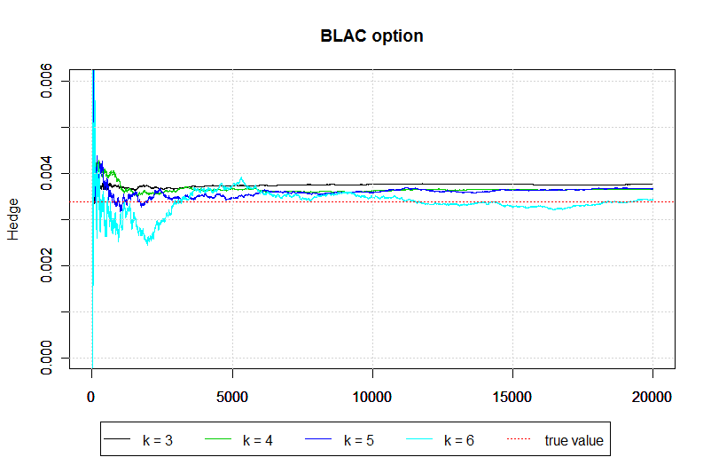
For comparison purposes with Bernis, Gobet and Kohatsu-Higa [1], we consider d=5d=5 underlying assets, r=0%r=0\% for the interest rate and T=1T=1 year for the maturity time. For each asset, we set initial values S0i=100;1i5S^{i}_{0}=100;~1\leq i\leq 5 and we compute the hedging strategy with respect to the first asset S1S^{1} with discretization level k=3,4,5,6k=3,4,5,6 and 2000020000 simulations.

Following the work [1], we consider the volatilities of the assets given by σ1=35%\|\sigma^{1}\|=35\%, σ2=35%\|\sigma^{2}\|=35\%, σ3=38%\|\sigma^{3}\|=38\%, σ4=35%\|\sigma^{4}\|=35\% and σ5=40%\|\sigma^{5}\|=40\%, the correlation matrix defined by ρij=0,4\rho_{ij}=0,4 for iji\neq j, where σi=(σi1,,σi5)\sigma^{i}=(\sigma_{i1},\cdots,\sigma_{i5})^{\top} and we use the barrier level L=76L=76. Table 1 provides the numerical results based on the algorithm described in Section 5 for the pointwise hedging strategy θH\theta^{H}. Due to Theorem 7.2, we expect that when the discretization level kk increases, we obtain results closer to the true value and this is what we find in our Monte Carlo experiments. The standard deviation and percentage %\% error in Table 1 are related to the average of the hedging strategies calculated by Monte Carlo and the difference between the true and the estimated hedging value, respectively.

k Result St. error True value Diference %\% error
33 0.003760.00376 2.37×1052.37\times 10^{-5} 0.003380.00338 0.000380.00038 11.15%11.15\%
44 0.003650.00365 4.80×1054.80\times 10^{-5} 0.003380.00338 0.000270.00027 8.03%8.03\%
55 0.003660.00366 9.31×1059.31\times 10^{-5} 0.003380.00338 0.000280.00028 8.35%8.35\%
66 0.003420.00342 1.82×1041.82\times 10^{-4} 0.003380.00338 0.000040.00004 1.29%1.29\%
Table 1. Monte Carlo hedging strategy of a BLAC down and out option for a 5-dimensional Black-Scholes model.

In Figure 1, we plot the average hedging estimates with respect to the number of simulations. One should notice that when kk increases, the standard error also increases, which suggests more simulations for higher values of kk.

Refer to caption
Figure 1. Monte Carlo hedging strategy of a BLAC down and out option for a 5-dimensional Black-Scholes model.

6.2. Hedging Errors.

Next, we present some hedging error results for two well-known non-constant volatility models: The constant elasticity of variance (CEV) model and the classical Heston stochastic volatility model [13]. The typical examples we have in mind are the generalized Föllmer-Schweizer, local risk minimization and mean variance hedging strategies, where the optimal hedging strategies are computed by means of the minimal martingale measure and the variance optimal martingale measure, respectively. We analyze digital and one-touch one-dimensional European-type contingent claims as follows

Digital option:H=11{ST<95},One-touch option:H=11{maxt[0,T]St>105}.\textbf{Digital option:}~~H=1\!\!1_{\{S_{T}<95\}},\quad\textbf{One-touch option:}~~H=1\!\!1_{\{\max_{t\in[0,T]}S_{t}>105\}}.

By using the algorithm described in Section 5, we compute the error committed by approximating the payoff HH by 𝔼^[H]+i=0n1θ^ti,0k,H(Sti,ti+1tiSti,0)\widehat{\mathbb{E}_{\mathbb{Q}}}[H]+\sum_{i=0}^{n-1}\hat{\theta}^{k,H}_{t_{i},0}(S_{t_{i},t_{i+1}-t_{i}}-S_{t_{i},0}). This error will be called hedging error. The computation of this error is summarized in the following steps:

  1. (1)

    We first simulate paths under the physical measure and compute the payoff HH.

  2. (2)

    Then, we consider some deterministic partition of the interval [0,T] into nn points t0,t1,,tn1t_{0},t_{1},\ldots,t_{n-1} such that ti+1ti=Tnt_{i+1}-t_{i}=\frac{T}{n}, for i=0,,n1i=0,\ldots,n-1.

  3. (3)

    One simulates at time t0=0t_{0}=0 the option price 𝔼^[H]\widehat{\mathbb{E}_{\mathbb{Q}}}[H] and the initial hedging estimate θ^0,0k,H\hat{\theta}^{k,H}_{0,0} from (5.2), (5.3) and (5.4) under a fixed e\mathbb{Q}\in\mathcal{M}^{e} following the algorithm described in Section 5.

  4. (4)

    We simulate θ^ti,0k,H\hat{\theta}^{k,H}_{t_{i},0} by means of the shifting argument based on the strong Markov property of the Brownian motion as described in Section 4.1.

  5. (5)

    We compute H^\hat{H} by

    (6.1) H^:=𝔼^[H]+i=0n1θ^ti,0k,H(Sti,ti+1tiSti,0).\hat{H}:=\widehat{\mathbb{E}_{\mathbb{Q}}}[H]+\sum_{i=0}^{n-1}\hat{\theta}^{k,H}_{t_{i},0}(S_{t_{i},t_{i+1}-t_{i}}-S_{t_{i},0}).
  6. (6)

    Finally, the hedging error estimate γ\gamma and the percentual error eγe_{\gamma} are given by γ:=HH^\gamma:=H-\hat{H} and eγ:=100×γ/𝔼^[H]e_{\gamma}:=100\times\gamma/\widehat{\mathbb{E}_{\mathbb{Q}}}[H], respectively.

Remark 6.1.

When no locally-risk minimizing strategy is available, we also expect to obtain low hedging errors when dealing with generalized Föllmer-Schweizer decompositions due to the orthogonal martingale decomposition. In the mean variance hedging case, two terms appear in the optimal hedging strategy: the pure hedging component θH,~\theta^{H,\tilde{\mathbb{P}}} of the GKW decomposition under the optimal variance martingale measure ~\tilde{\mathbb{P}} and ζ~\tilde{\zeta} as described by (1.4) and (1.5). For the Heston model, ζ~\tilde{\zeta} was explicitly calculated by Hobson [14]. We have used his formula in our numerical simulations jointly with θ^k,H\hat{\theta}^{k,H} under ~\tilde{\mathbb{P}} in the calculation of the mean variance hedging errors. See expression (6.4) for details.

6.2.1. Constant Elasticity of Variance (CEV) model

The discounted risky asset price process described by the CEV model under the physical measure is given by

(6.2) dSt=St[(btrt)dt+σSt(β2)/2dBt],S0=s,dS_{t}=S_{t}\left[(b_{t}-r_{t})dt+\sigma S^{(\beta-2)/2}_{t}dB_{t}\right],\quad S_{0}=s,

where BB is a \mathbb{P}-Brownian motion. The instantaneous sharpe ratio is ψt=btrtσSt(β2)/2\psi_{t}=\frac{b_{t}-r_{t}}{\sigma S^{(\beta-2)/2}_{t}} such that the model can be rewritten as

(6.3) dSt=σtStβ/2dWtdS_{t}=\sigma_{t}S^{\beta/2}_{t}dW_{t}

where WW is a \mathbb{Q}-Brownian motion and \mathbb{Q} is the equivalent local martingale measure. For both the digital and one-touch options, we consider the parameters r=0r=0 for the interest rate, T=1T=1 (month) for the maturity time, σ=0.2\sigma=0.2, S0=100S_{0}=100 and β=1.6\beta=1.6 such that the constant of elasticity is 0.4-0.4. We simulate the hedging error along [0,T][0,T] considering discretization levels k=3,4k=3,4, and 11 and 22 hedging strategies per day, which means approximately 2222 and 4444 hedging strategies, respectively, along the interval [0,T][0,T]. From Corollary 4.2, we know that this procedure is consistent. For the digital option, we also recall that the hedging strategy has continuous paths up to some stopping time (see Zhang [27]) so that Theorem 7.2 and Remark 7.2 apply accordingly. The hedging error results for the digital and one-touch options are summarized in Tables 2 and 3, respectively. The standard deviations are related to the hedging errors.

Simulations k Hedges/day Hedging error γ\gamma St. dev. Price % Error eγe_{\gamma}
200200 33 11 0.02696-0.02696 0.17500.1750 0.28640.2864 9.41%9.41\%
200200 33 22 0.00473-0.00473 0.14510.1451 0.28640.2864 1.65%1.65\%
200200 44 11 0.004940.00494 0.15620.1562 0.27590.2759 1.79%1.79\%
200200 44 22 0.00291-0.00291 0.15220.1522 0.27600.2760 1.05%1.05\%
Table 2. Hedging error of a digital option for the CEV model.
Simulations k Hedges/day Hedging error γ\gamma St. dev. Price % Error eγe_{\gamma}
600600 33 11 0.04170.0417 0.17270.1727 0.48040.4804 8.68%8.68\%
600600 33 22 0.04240.0424 0.14130.1413 0.48040.4804 8.82%8.82\%
600600 44 11 0.01440.0144 0.17700.1770 0.50610.5061 2.84%2.84\%
600600 44 22 0.01250.0125 0.11680.1168 0.50600.5060 2.47%2.47\%
Table 3. Hedging error of one-touch option for the CEV model.

6.2.2. Heston’s Stochastic Volatility Model

Here we consider two types of hedging methodologies: Local-risk minimization and mean variance hedging strategies as described in the Introduction and Remark 6.1. The Heston dynamics of the discounted price under the physical measure is given by

{dSt=St(btrt)Σtdt+StΣtdBt(1)dΣt=2κ(θΣt)dt+2σΣtdZt,0tT,\left\{\begin{array}[]{l}dS_{t}=S_{t}(b_{t}-r_{t})\Sigma_{t}dt+S_{t}\sqrt{\Sigma_{t}}dB^{(1)}_{t}\\ d\Sigma_{t}=2\kappa(\theta-\Sigma_{t})dt+2\sigma\sqrt{\Sigma_{t}}dZ_{t},0\leq t\leq T,\end{array}\right.

where Z=ρB(1)+ρ¯Bt(2)Z=\rho B^{(1)}+\bar{\rho}B^{(2)}_{t}, ρ¯=1ρ2\bar{\rho}=\sqrt{1-\rho^{2}}, with (B(1)B(2))(B^{(1)}B^{(2)}) two independent \mathbb{P}-Brownian motions and κ,m,β0,μ\kappa,m,\beta_{0},\mu are suitable constants in order to have a well-defined Markov process (see e.g Heston [13]). Alternatively, we can rewrite the dynamics as

{dSt=StYt2(btrt)dt+StYtdBt(1)dYt=κ(mYtYt)dt+σdZt,0tT,\left\{\begin{array}[]{l}dS_{t}=S_{t}Y^{2}_{t}(b_{t}-r_{t})dt+S_{t}Y_{t}dB^{(1)}_{t}\\ dY_{t}=\kappa\Bigg{(}\frac{m}{Y_{t}}-Y_{t}\Bigg{)}dt+\sigma dZ_{t},~0\leq t\leq T,\end{array}\right.

where Y=ΣtY=\sqrt{\Sigma_{t}} and m=θσ22κm=\theta-\frac{\sigma^{2}}{2\kappa}.

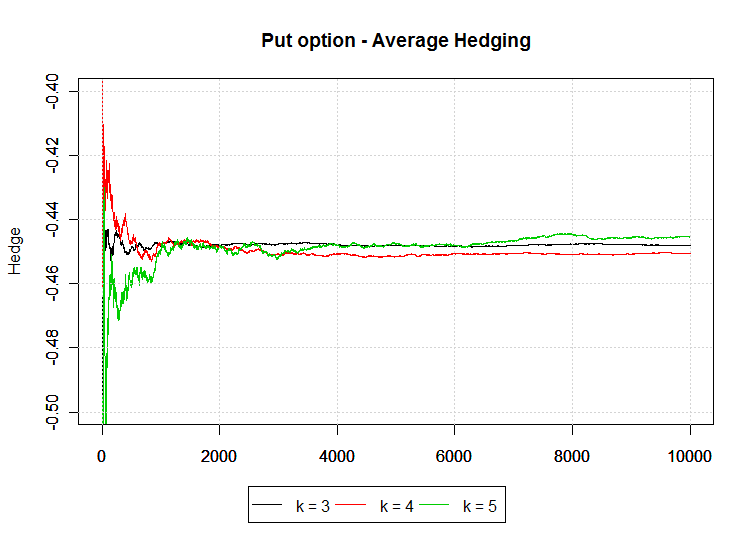
Local-Risk Minimization. For comparison purposes with Heath, Platen and Schweizer [12], we consider the hedging of a European put option HH written on a Heston model with correlation parameter ρ=0\rho=0. We set S0=100S_{0}=100, strike price K=100K=100, T=1T=1 (month) and we use discretization levels k=3,4k=3,4 and 55. We set the parameters κ=2.5\kappa=2.5, θ=0.04\theta=0.04, ρ=0\rho=0, σ=0.3\sigma=0.3, r=0r=0 and Y0=0.02Y_{0}=0.02. In this case, the hedging strategy θH,^\theta^{H,\hat{\mathbb{P}}} based on the local-risk-minimization methodology is bounded with continuous paths so that Theorem 7.2 applies to this case. Moreover, as described by Heath, Platen and Schweizer [12], θH,^\theta^{H,\hat{\mathbb{P}}} can be obtained by a PDE numerical analysis.

Table 4 presents the results of the hedging strategy θ^0,0k,H\hat{\theta}^{k,H}_{0,0} by using the algorithm described in Section 5. Figure 2 provides the Monte Carlo hedging strategy with respect to the number of simulations of order 1000010000. We notice that our results agree with the results obtained by Heath, Platen and Schweizer [12] by PDE methods. In this case, the true value of the hedging at time t=0t=0 is approximately 0.44-0.44. The standard errors in Table 4 are related to the hedging and prices computed, respectively, from the Monte Carlo method described in Section 5.

k Hedging Standard error Monte Carlo price Standard error
33 0.4480-0.4480 6.57×1046.57\times 10^{-4} 10.41710.417 5.00×1035.00\times 10^{-3}
44 0.4506-0.4506 1.28×1031.28\times 10^{-3} 10.42210.422 3.35×1033.35\times 10^{-3}
55 0.4453-0.4453 2.54×1032.54\times 10^{-3} 10.40910.409 2.75×1032.75\times 10^{-3}
Table 4. Monte Carlo local-risk minimization hedging strategy of a European put option with Heston model.
Refer to caption
Figure 2. Monte Carlo local-risk minimization hedging strategy of a European put option with Heston model.

Hedging with generalized Föllmer-Schweizer decomposition for one-touch option. Based on Corollary 4.2, we also present the hedging error associated to one-touch options for a Heston model with non-zero correlation. We simulate the hedging error along the interval [0,1][0,1] using k=3,4k=3,4 as discretization levels and 11 and 22 hedging strategies per day with parameters κ=3.63\kappa=3.63, θ=0.04\theta=0.04, ρ=0.53\rho=-0.53, σ=0.3\sigma=0.3, r=0r=0, b=0.01b=0.01, Y0=0.3Y_{0}=0.3 and S0=100S_{0}=100 where the barrier is 105105. The hedging error result for the one-touch option is summarized in Table 5. The standard deviations in Table 5 are related to the hedging error.

To our best knowledge, there is no result about the existence of locally-risk minimizing hedging strategies for one-touch options written on a Heston model with nonzero correlation. As pointed out in Remark 6.1, it is expected that pure hedging strategies based on the generalized Föllmer-Schweizer decomposition mitigate very-well the hedging error. This is what we get in the simulation results.

Simulations k Hedges/day Hedging error γ\gamma St. dev. Price % error eγe_{\gamma}
600600 33 11 0.04090.0409 0.24520.2452 0.73990.7399 5.53%5.53\%
600600 33 22 0.03160.0316 0.24500.2450 0.73970.7397 4.27%4.27\%
600600 44 11 0.02680.0268 0.28420.2842 0.77350.7735 3.46%3.46\%
600600 44 22 0.01910.0191 0.26050.2605 0.77380.7738 2.47%2.47\%
Table 5. Hedging error with generalized Föllmer-Schweizer decomposition: One-touch option with Heston model.

Mean variance hedging strategy. Here we present the hedging errors associated to one-touch options written on a Heston model with non-zero correlation under the mean variance methodology. Again, we simulate the hedging error along the interval [0,1][0,1] using k=3,4k=3,4 as discritization levels and 11 and 22 hedging strategies per day with parameters r=0r=0, b=0.01b=0.01, κ=3.63\kappa=3.63, θ=0.04\theta=0.04, ρ=0.53\rho=-0.53, σ=0.3\sigma=0.3, Y0=0.3Y_{0}=0.3 and S0=100S_{0}=100 with barrier 105. The computation of the optimal hedging strategy follows from Remark 6.1. The quantity ζ~\tilde{\zeta} is not related to the GKW decomposition but it is described by Theorem 1.1 in Hobson [14] as follows. The process ζ~\tilde{\zeta} appearing in (1.4) and (1.5) is given by

(6.4) ζ~t=Z~0ρσF(Tt)Z~0b;0tT,\tilde{\zeta}_{t}=\tilde{Z}_{0}\rho\sigma F(T-t)-\tilde{Z}_{0}b;~0\leq t\leq T,

where FF is given by (see case 2 of Prop. 5.1 in Hobson [14])

F(t)=CAtanh(ACt+tanh1(ABC))B;0tT,F(t)=\frac{C}{A}\tanh\left(ACt+\tanh^{-1}\left(\frac{AB}{C}\right)\right)-B;~0\leq t\leq T,

with A=|12ρ2|σ2A=\sqrt{|1-2\rho^{2}|\sigma^{2}}, B=κ+2ρσbσ2|12ρ2|B=\frac{\kappa+2\rho\sigma b}{\sigma^{2}|1-2\rho^{2}|} and C=|D|C=\sqrt{|D|} where D=2b2+(κ+2ρσb)2)σ2(12ρ2)D=2b^{2}+\frac{(\kappa+2\rho\sigma b)^{2})}{\sigma^{2}(1-2\rho^{2})}. The initial condition Z~0\tilde{Z}_{0} is given by

Z~0=Y022F(T)+κθ0TF(s)𝑑s.\tilde{Z}_{0}=\frac{Y_{0}^{2}}{2}F(T)+\kappa\theta\int_{0}^{T}F(s)ds.

The hedging error results are summarized in Table 6 where the standard deviations are related to the hedging error. In comparison with the local-risk minimization methodology, the results show smaller percentual errors when kk increases. Also, in all the cases, we had smaller values of the standard deviation which suggests the mean variance methodology provides more accurate values of the hedging strategy.

Simulations k Hedges/day Hedging error γ\gamma St. dev. Price % error eγe_{\gamma}
600600 33 11 0.06890.0689 0.16880.1688 0.73390.7339 9.39%9.39\%
600600 33 22 0.05920.0592 0.13440.1344 0.73390.7339 8.07%8.07\%
600600 44 11 0.02130.0213 0.18460.1846 0.77660.7766 2.74%2.74\%
600600 44 22 0.01610.0161 0.12780.1278 0.77650.7765 2.07%2.07\%
Table 6. Hedging error in the mean variance hedging methodology for one-touch option with Heston model.

7. Appendix

This appendix provides a deeper understanding of the Monte Carlo algorithm proposed in this work when the representation (ϕH,S,ϕH,I)(\phi^{H,S},\phi^{H,I}) in (3.6) admits additional integrability and path smoothness assumptions. We present stronger approximations which complement the asymptotic result given in Theorem 3.1. Uniform-type weak and strong pointwise approximations for θH\theta^{H} are presented and they validate the numerical experiments in Tables 1 and 4 in Section 6. At first, we need of some technical lemmas.

Lemma 7.1.

Suppose that ϕH=(ϕH,1,,ϕH,p)\phi^{H}=(\phi^{H,1},\ldots,\phi^{H,p}) is a pp-dimensional progressive process such that 𝔼sup0tTϕtHp2<\mathbb{E}\sup_{0\leq t\leq T}\|\phi^{H}_{t}\|^{2}_{\mathbb{R}^{p}}<\infty. Then, the following identity holds

(7.1) ΔδkXT1k,j=𝔼[0T1k,jϕsH,j𝑑Ws(j)T1k,jk]a.s;j=1,,p;k1.\Delta\delta^{k}X_{T^{k,j}_{1}}=\mathbb{E}\left[\int_{0}^{T^{k,j}_{1}}\phi^{H,j}_{s}dW^{(j)}_{s}\mid\mathcal{F}^{k}_{T^{k,j}_{1}}\right]~a.s;~j=1,\ldots,p;k\geq 1.
Proof.

It is sufficient to prove for p=2p=2 since the argument for p>2p>2 easily follows from this case. Let \mathcal{H} be the linear space constituted by the bounded 2\mathbb{R}^{2}-valued 𝔽\mathbb{F}-progressive processes ϕ=(ϕ1,ϕ2)\phi=(\phi^{1},\phi^{2}) such that (7.1) holds with X=X0+0ϕs1𝑑Ws(1)+0ϕs2𝑑Ws(2)X=X_{0}+\int_{0}^{\cdot}\phi^{1}_{s}dW^{(1)}_{s}+\int_{0}^{\cdot}\phi^{2}_{s}dW^{(2)}_{s} where X00X_{0}\in\mathcal{F}_{0}. Let 𝒰\mathcal{U} be the class of stochastic intervals of the form [[S,+[[[[S,+\infty[[ where SS is a 𝔽\mathbb{F}-stopping time. We claim that ϕ=(11[[S,+[[,11[[J,+[[)\phi=\big{(}1\!\!1_{[[S,+\infty[[},1\!\!1_{[[J,+\infty[[}\big{)}\in\mathcal{H} for every 𝔽\mathbb{F}-stopping times SS and JJ. In order to check (7.1) for such ϕ\phi, we only need to show for j=1j=1 since the argument for j=2j=2 is the same. With a slight abuse of notation, any sub-sigma algebra of T\mathcal{F}_{T} of the form Ω1𝒢\Omega^{*}_{1}\otimes\mathcal{G} will be denoted by 𝒢\mathcal{G} where Ω1\Omega^{*}_{1} is the trivial sigma-algebra on the first copy Ω1\Omega_{1}.

At first, we split Ω=n=1{Tnk=T1k,1}\Omega=\bigcup_{n=1}^{\infty}\{T^{k}_{n}=T^{k,1}_{1}\} and we make the argument on the sets {Tnk=T1k,1};n1\{T^{k}_{n}=T^{k,1}_{1}\};~n\geq 1. In this case, we know that T1k,1k=T1k,1k,1Tn1k,2k,2\mathcal{F}^{k}_{T^{k,1}_{1}}=\mathcal{F}^{k,1}_{T^{k,1}_{1}}\otimes\mathcal{F}^{k,2}_{T^{k,2}_{n-1}}\  a.s and

ΔδkXT1k,j=Δδk(WT1k,1(1)WS(1))11{S<T1k,1}+Δδk(WT1k,1(2)WJ(2))11{J<T1k,1}.\Delta\delta^{k}X_{T^{k,j}_{1}}=\Delta\delta^{k}\left(W^{(1)}_{T^{k,1}_{1}}-W^{(1)}_{S}\right)1\!\!1_{\{S<T^{k,1}_{1}\}}+\Delta\delta^{k}\left(W^{(2)}_{T^{k,1}_{1}}-W^{(2)}_{J}\right)1\!\!1_{\{J<T^{k,1}_{1}\}}.

The independence between W(1)W^{(1)} and W(2)W^{(2)} and the independence of the Brownian motion increments yield

Δδk(WT1k,1(2)WJ(2))\displaystyle\Delta\delta^{k}\left(W^{(2)}_{T^{k,1}_{1}}-W^{(2)}_{J}\right) =𝔼(WT1k,1(2)WJ(2)T1k,1k)𝔼(WT1k,1(2)WJ(2)Tn1kk)\displaystyle=\mathbb{E}\left(W^{(2)}_{T^{k,1}_{1}}-W^{(2)}_{J}\mid\mathcal{F}^{k}_{T^{k,1}_{1}}\right)-\mathbb{E}\left(W^{(2)}_{T^{k,1}_{1}}-W^{(2)}_{J}\mid\mathcal{F}^{k}_{T^{k}_{n-1}}\right)
=𝔼(WT1k,1(2)WJ(2)T1k,1k,1Tn1k,2k,2)=𝔼(WT1k,1(2)WJ(2)σ{T1k,1}Tn1k,2k,2)\displaystyle=\mathbb{E}\left(W^{(2)}_{T^{k,1}_{1}}-W^{(2)}_{J}\mid\mathcal{F}^{k,1}_{T^{k,1}_{1}}\otimes\mathcal{F}^{k,2}_{T^{k,2}_{n-1}}\right)=\mathbb{E}\left(W^{(2)}_{T^{k,1}_{1}}-W^{(2)}_{J}\mid\sigma\{T^{k,1}_{1}\}\otimes\mathcal{F}^{k,2}_{T^{k,2}_{n-1}}\right)
=𝔼(WT1k,1(2)WJ(2)Tn1k,2k,2)=0a.s\displaystyle=\mathbb{E}\left(W^{(2)}_{T^{k,1}_{1}}-W^{(2)}_{J}\mid\mathcal{F}^{k,2}_{T^{k,2}_{n-1}}\right)=0\quad a.s

on the set {Tn1kJ<Tnk=T1k,1}\{T_{n-1}^{k}\leq J<T_{n}^{k}=T^{k,1}_{1}\}. We also have,

Δδk(WT1k,1(2)WJ(2))\displaystyle\Delta\delta^{k}\left(W^{(2)}_{T^{k,1}_{1}}-W^{(2)}_{J}\right) =𝔼(WT1k,1(2)WJ(2)T1k,1k)𝔼(WT1k,1(2)WJ(2)Tn1kk)\displaystyle=\mathbb{E}\left(W^{(2)}_{T^{k,1}_{1}}-W^{(2)}_{J}\mid\mathcal{F}^{k}_{T^{k,1}_{1}}\right)-\mathbb{E}\left(W^{(2)}_{T^{k,1}_{1}}-W^{(2)}_{J}\mid\mathcal{F}^{k}_{T^{k}_{n-1}}\right)
=𝔼(WT1k,1(2)WJ(2)T1k,1k,1Tn1k,2k,2)𝔼(WTn1k(2)WJ(2)Tn1k,2k,2)\displaystyle=\mathbb{E}\left(W^{(2)}_{T^{k,1}_{1}}-W^{(2)}_{J}\mid\mathcal{F}^{k,1}_{T^{k,1}_{1}}\otimes\mathcal{F}^{k,2}_{T^{k,2}_{n-1}}\right)-\mathbb{E}\left(W^{(2)}_{T^{k}_{n-1}}-W^{(2)}_{J}\mid\mathcal{F}^{k,2}_{T^{k,2}_{n-1}}\right)
=𝔼(WT1k,1(2)WJ(2)σ{T1k,1}Tn1k,2k,2)𝔼(WTn1k(2)WJ(2)Tn1k,2k,2)\displaystyle=\mathbb{E}\left(W^{(2)}_{T^{k,1}_{1}}-W^{(2)}_{J}\mid\sigma\{T^{k,1}_{1}\}\otimes\mathcal{F}^{k,2}_{T^{k,2}_{n-1}}\right)-\mathbb{E}\left(W^{(2)}_{T^{k}_{n-1}}-W^{(2)}_{J}\mid\mathcal{F}^{k,2}_{T^{k,2}_{n-1}}\right)
=𝔼(WTn1k(2)WJ(2)Tn1k,2k,2)𝔼(WTn1k(2)WJ(2)Tn1k,2k,2)=0,\displaystyle=\mathbb{E}\left(W^{(2)}_{T^{k}_{n-1}}-W^{(2)}_{J}\mid\mathcal{F}^{k,2}_{T^{k,2}_{n-1}}\right)-\mathbb{E}\left(W^{(2)}_{T^{k}_{n-1}}-W^{(2)}_{J}\mid\mathcal{F}^{k,2}_{T^{k,2}_{n-1}}\right)=0,

on the set {J<Tn1k}\{J<T_{n-1}^{k}\}. By construction T1k,1k=T1k,1k,1Tn1k,2k,2\mathcal{F}^{k}_{T^{k,1}_{1}}=\mathcal{F}^{k,1}_{T^{k,1}_{1}}\otimes\mathcal{F}^{k,2}_{T^{k,2}_{n-1}}\  a.s and again the independence between W(1)W^{(1)} and W(2)W^{(2)} yields

Δδk(WT1k,1(1)WS(1))\displaystyle\Delta\delta^{k}\left(W^{(1)}_{T^{k,1}_{1}}-W^{(1)}_{S}\right) =𝔼(WT1k,1(1)WS(1)T1k,1k)𝔼(WT1k,1(1)WS(1)Tn1kk)\displaystyle=\mathbb{E}\left(W^{(1)}_{T^{k,1}_{1}}-W^{(1)}_{S}\mid\mathcal{F}^{k}_{T^{k,1}_{1}}\right)-\mathbb{E}\left(W^{(1)}_{T^{k,1}_{1}}-W^{(1)}_{S}\mid\mathcal{F}^{k}_{T^{k}_{n-1}}\right)
=𝔼(WT1k,1(1)WS(1)T1k,1k)\displaystyle=\mathbb{E}\left(W^{(1)}_{T^{k,1}_{1}}-W^{(1)}_{S}\mid\mathcal{F}^{k}_{T^{k,1}_{1}}\right)

on {Tn1kS<Tnk=T1k,1}\{T_{n-1}^{k}\leq S<T_{n}^{k}=T^{k,1}_{1}\}. Similarly,

Δδk(WT1k,1(1)WS(1))\displaystyle\Delta\delta^{k}\left(W^{(1)}_{T^{k,1}_{1}}-W^{(1)}_{S}\right) =𝔼(WT1k,1(1)WS(1)T1k,1k)𝔼(WT1k,1(1)WS(1)Tn1kk)\displaystyle=\mathbb{E}\left(W^{(1)}_{T^{k,1}_{1}}-W^{(1)}_{S}\mid\mathcal{F}^{k}_{T^{k,1}_{1}}\right)-\mathbb{E}\left(W^{(1)}_{T^{k,1}_{1}}-W^{(1)}_{S}\mid\mathcal{F}^{k}_{T^{k}_{n-1}}\right)
=𝔼(WT1k,1(1)WS(1)T1k,1k)𝔼(WTn1k(1)WS(1)Tn1kk,2)\displaystyle=\mathbb{E}\left(W^{(1)}_{T^{k,1}_{1}}-W^{(1)}_{S}\mid\mathcal{F}^{k}_{T^{k,1}_{1}}\right)-\mathbb{E}\left(W^{(1)}_{T^{k}_{n-1}}-W^{(1)}_{S}\mid\mathcal{F}^{k,2}_{T^{k}_{n-1}}\right)
=𝔼(WT1k,1(1)WS(1)T1k,1k)𝔼(WTn1k(1)Tn1kk,2)+𝔼(WS(1)Tn1kk,2)\displaystyle=\mathbb{E}\left(W^{(1)}_{T^{k,1}_{1}}-W^{(1)}_{S}\mid\mathcal{F}^{k}_{T^{k,1}_{1}}\right)-\mathbb{E}\left(W^{(1)}_{T^{k}_{n-1}}\mid\mathcal{F}^{k,2}_{T^{k}_{n-1}}\right)+\mathbb{E}\left(W^{(1)}_{S}\mid\mathcal{F}^{k,2}_{T^{k}_{n-1}}\right)
=𝔼(WT1k,1(1)WS(1)T1k,1k)+𝔼(WS(1)Tn1kk,2)\displaystyle=\mathbb{E}\left(W^{(1)}_{T^{k,1}_{1}}-W^{(1)}_{S}\mid\mathcal{F}^{k}_{T^{k,1}_{1}}\right)+\mathbb{E}\left(W^{(1)}_{S}\mid\mathcal{F}^{k,2}_{T^{k}_{n-1}}\right)

on {S<Tn1k}\{S<T_{n-1}^{k}\}. By assumption SS is an 𝔽\mathbb{F}-stopping time, where 𝔽\mathbb{F} is a product filtration. Hence, 𝔼(WS(1)|Tn1kk,2)=0\mathbb{E}\big{(}W^{(1)}_{S}|\mathcal{F}^{k,2}_{T^{k}_{n-1}}\big{)}=0 a.s on {S<Tn1k}\{S<T_{n-1}^{k}\}.

Summing up the above identities, we shall conclude (11[[S,+[[,11[[J,+[[)\big{(}1\!\!1_{[[S,+\infty[[},1\!\!1_{[[J,+\infty[[}\big{)}\in\mathcal{H}. In particular, the constant process (1,1)(1,1)\in\mathcal{H} and if ϕn\phi^{n} is a sequence in \mathcal{H} such that ϕnϕ\phi^{n}\rightarrow\phi a.s Leb×Leb\times\mathbb{Q} with ϕ\phi bounded, then a routine application of Burkhölder inequality shows that ϕ\phi\in\mathcal{H}. Since 𝒰\mathcal{U} generates the optional sigma-algebra then we shall apply the monotone class theorem and, by localization, we may conclude the proof.

Lemma 7.2.

Let BB be a one-dimensional Brownian motion and Snk:=inf{t>Sn1k;|BtBSn1k|=2k}S^{k}_{n}:=\inf\{t>S^{k}_{n-1};|B_{t}-B_{S^{k}_{n-1}}|=2^{-k}\} with S0k=0a.sS^{k}_{0}=0~a.sn1n\geq 1. If φ\varphi is an absolutely continuous and non-negative adapted process then there exists a deterministic constant CC which does not depend on m,k1m,k\geq 1 such that

|Sm1kSmkφt𝑑Bt|211{SmkT}Csup0tT|φt|222ka.s;k,m1.\Bigg{|}\int_{S^{k}_{m-1}}^{S^{k}_{m}}\varphi_{t}dB_{t}\Bigg{|}^{2}1\!\!1_{\{S^{k}_{m}\leq T\}}\leq C\sup_{0\leq t\leq T}|\varphi_{t}|^{2}2^{-2k}~a.s;~k,m\geq 1.
Proof.

For given m,k1m,k\geq 1, Young inequality and integration by parts yield

|Sm1kSmkφt𝑑Bt|2\displaystyle\Bigg{|}\int_{S^{k}_{m-1}}^{S^{k}_{m}}\varphi_{t}dB_{t}\Bigg{|}^{2} C{|φSmk|2|BSmk|2+|φSm1k|2|BSm1k|2+|Sm1kSmkBt𝑑φt|2}\displaystyle\leq C\Big{\{}|\varphi_{S^{k}_{m}}|^{2}|B_{S^{k}_{m}}|^{2}+|\varphi_{S^{k}_{m-1}}|^{2}|B_{S^{k}_{m-1}}|^{2}+\big{|}\int_{S^{k}_{m-1}}^{S^{k}_{m}}B_{t}d\varphi_{t}\big{|}^{2}\Big{\}}
C22ksup0tT|φt|2+CsupSm1ktSmk|Bt|2|Var(φ)SmkVar(φ)Sm1k|2\displaystyle\leq C2^{-2k}\sup_{0\leq t\leq T}|\varphi_{t}|^{2}+C\sup_{S^{k}_{m-1}\leq t\leq S^{k}_{m}}|B_{t}|^{2}|Var(\varphi)_{S^{k}_{m}}-Var(\varphi)_{S^{k}_{m-1}}|^{2}
C22ksup0tT|φt|2+C22k|Var(φ)SmkVar(φ)Sm1k|2\displaystyle\leq C2^{-2k}\sup_{0\leq t\leq T}|\varphi_{t}|^{2}+C2^{-2k}|Var(\varphi)_{S^{k}_{m}}-Var(\varphi)_{S^{k}_{m-1}}|^{2}
=C22ksup0tT|φt|2+C22k|φSmkφSm1k|2\displaystyle=C2^{-2k}\sup_{0\leq t\leq T}|\varphi_{t}|^{2}+C2^{-2k}|\varphi_{S^{k}_{m}}-\varphi_{S^{k}_{m-1}}|^{2}
C22ksup0tT|φt|2a.son{SmkT},\displaystyle\leq C2^{-2k}\sup_{0\leq t\leq T}|\varphi_{t}|^{2}~a.s~\text{on}~\{S^{k}_{m}\leq T\},

for some constant CC which does not depend on m,k1m,k\geq 1. ∎

Lemma 7.3.

Assume that ϕH,jB2(𝔽)\phi^{H,j}\in\text{B}^{2}(\mathbb{F}) for some j=1,,pj=1,\ldots,p. Then there exists a constant CC such that

supk1𝔼sup0tT|𝐃k,jXt|2C𝔼sup0tT|ϕH,j|2.\sup_{k\geq 1}\mathbb{E}\sup_{0\leq t\leq T}|\mathbf{D}^{k,j}X_{t}|^{2}\leq C\mathbb{E}\sup_{0\leq t\leq T}|\phi^{H,j}|^{2}.
Proof.

By repeating the argument employed in Lemma 7.1 for k1k\geq 1n>1n>1 and j{1,,p}j\in\{1,\ldots,p\}, we shall write

𝐃k,jXt=𝔼[1ΔATnk,jk,jTn1k,jTnk,jϕtH,j𝑑Wt(j)|Tn1k,jk]a.son{Tn1k,j<tTnk,j}.\mathbf{D}^{k,j}X_{t}=\mathbb{E}\Bigg{[}\frac{1}{\Delta A^{k,j}_{T^{k,j}_{n}}}\int_{T^{k,j}_{n-1}}^{T^{k,j}_{n}}\phi^{H,j}_{t}dW^{(j)}_{t}\big{|}\mathcal{F}^{k}_{T^{k,j}_{n-1}}\Bigg{]}~a.s~\text{on}~\{T^{k,j}_{n-1}<t\leq T^{k,j}_{n}\}.

Doob maximal inequalities combined with Jensen inequality yield

(7.2) 𝔼sup0tT|𝐃k,jXt|2C22k𝔼supn1|Tn1k,jTnk,jϕtH,j𝑑Wt(j)|211{Tnk,jT},\mathbb{E}\sup_{0\leq t\leq T}|\mathbf{D}^{k,j}X_{t}|^{2}\leq C2^{2k}\mathbb{E}\sup_{n\geq 1}\Bigg{|}\int_{T^{k,j}_{n-1}}^{T^{k,j}_{n}}\phi^{H,j}_{t}dW^{(j)}_{t}\Bigg{|}^{2}1\!\!1_{\{T^{k,j}_{n}\leq T\}},

for k1k\geq 1 and for some positive constant CC. Now, we need a path-wise argument in order to estimate the right-hand side of (7.2). For this, let us define

φt,j:=t1tϕsH,j𝑑s;1;0tT.\varphi^{\ell,j}_{t}:=\ell\int_{t-\frac{1}{\ell}}^{t}\phi^{H,j}_{s}ds;~\ell\geq 1;~0\leq t\leq T.

Lemma 7.2 and the fact that sup0tT|φt,j|2sup0tT|ϕtH,j|21\sup_{0\leq t\leq T}|\varphi^{\ell,j}_{t}|^{2}\leq\sup_{0\leq t\leq T}|\phi^{H,j}_{t}|^{2}~\forall\ell\geq 1 yield

(7.3) |Tn1k,jTnk,jφt,j𝑑Wt(j)|211{Tnk,jT}Csup0tT|ϕtH,j|222k;,n,k1,\Bigg{|}\int_{T^{k,j}_{n-1}}^{T^{k,j}_{n}}\varphi^{\ell,j}_{t}dW^{(j)}_{t}\Bigg{|}^{2}1\!\!1_{\{T^{k,j}_{n}\leq T\}}\leq C\sup_{0\leq t\leq T}|\phi^{H,j}_{t}|^{2}2^{-2k};~\ell,n,k\geq 1,

where CC is the constant in Lemma 7.2. Now, by applying Lemma 2.4 in Nutz [21], the estimate (7.3) and a routine localization procedure, the following estimate holds

|Tn1k,jTnk,jϕtH,j𝑑Wt(j)|211{Tnk,jT}Csup0tT|ϕtH,j|222k;k1,\Bigg{|}\int_{T^{k,j}_{n-1}}^{T^{k,j}_{n}}\phi^{H,j}_{t}dW^{(j)}_{t}\Bigg{|}^{2}1\!\!1_{\{T^{k,j}_{n}\leq T\}}\leq C\sup_{0\leq t\leq T}|\phi^{H,j}_{t}|^{2}2^{-2k};~k\geq 1,

and therefore

(7.4) 𝔼supn1|Tn1k,jTnk,jϕtH,j𝑑Wt(j)|211{Tnk,jT}C𝔼sup0tT|ϕtH,j|222kk1.\mathbb{E}\sup_{n\geq 1}\Bigg{|}\int_{T^{k,j}_{n-1}}^{T^{k,j}_{n}}\phi^{H,j}_{t}dW^{(j)}_{t}\Bigg{|}^{2}1\!\!1_{\{T^{k,j}_{n}\leq T\}}\leq C\mathbb{E}\sup_{0\leq t\leq T}|\phi^{H,j}_{t}|^{2}2^{-2k}~\forall k\geq 1.

The estimate (7.2) combined with (7.4) allow us to conclude the proof if ϕH,j0a.s(Leb×)\phi^{H,j}\geq 0~a.s~(Leb\times\mathbb{Q}). By splitting ϕH,j=ϕH,j,+ϕH,j,\phi^{H,j}=\phi^{H,j,+}-\phi^{H,j,-} into the negative and positive parts, we may conclude the proof of the lemma. ∎

The following result allows us to get a uniform-type weak convergence of 𝐃k,jX\mathbf{D}^{k,j}X under very mild integrability assumption.

Theorem 7.1.

Let HH be a \mathbb{Q}-square integrable contingent claim satisfying assumption (M) and assume that HH admits a representation ϕH\phi^{H} such that ϕH,jB2(𝔽)\phi^{H,j}\in\text{B}^{2}(\mathbb{F}) for some j{1,,p}j\in\{1,\ldots,p\}. Then

limk𝐃k,jX=ϕH,j\lim_{k\rightarrow\infty}\mathbf{D}^{k,j}X=\phi^{H,j}

weakly in B2(𝔽)\text{B}^{2}(\mathbb{F}).

Proof.

Let us fix j=1,,pj=1,\ldots,p. From Lemma 7.3, we know that {𝐃k,jX;k1}\{\mathbf{D}^{k,j}X;k\geq 1\} is bounded in B2(𝔽)\text{B}^{2}(\mathbb{F}) and therefore this set is weakly relatively compact in B2(𝔽)\text{B}^{2}(\mathbb{F}). By Eberlein Theorem, we also know that it is B2(𝔽)\text{B}^{2}(\mathbb{F})-weakly relatively sequentially compact. From Theorem 3.1,

limk𝐃k,jX=ϕH,j\lim_{k\rightarrow\infty}\mathbf{D}^{k,j}X=\phi^{H,j}

weakly in L2(Leb×)L^{2}(Leb\times\mathbb{Q}) and since B2\|\cdot\|_{\text{B}^{2}} is stronger than L2(Leb×)\|\cdot\|_{L^{2}(Leb\times\mathbb{Q})}, we necessarily have the full convergence

limk𝐃k,jX=ϕH,j\lim_{k\rightarrow\infty}\mathbf{D}^{k,j}X=\phi^{H,j}

in σ(B2,M2)\sigma(\text{B}^{2},\text{M}^{2}). ∎

Next, we analyze the pointwise strong convergence for our approximation scheme.

7.1. Strong Convergence under Mild Regularity

In this section, we provide a pointwise strong convergence result for GKW projectors under rather weak path regularity conditions. Let us consider the stopping times

τj:=inf{t>0;|Wt(j)|=1};j=1,,p,\tau^{j}:=\inf\big{\{}t>0;|W^{(j)}_{t}|=1\big{\}};~j=1,\ldots,p,

and we set

ψH,j(u):=𝔼|ϕτjuH,jϕ0H,j|2,foru0,j=1,p.\psi^{H,j}(u):=\mathbb{E}|\phi^{H,j}_{\tau^{j}u}-\phi^{H,j}_{0}|^{2},~\text{for}~u\geq 0,j=1\ldots,p.

Here, if uu satisfies τjuT\tau^{j}u\geq T we set ϕτjuH,j:=ϕTH,j\phi^{H,j}_{\tau^{j}u}:=\phi^{H,j}_{T} and for simplicity we assume that ψH,j(0)=0\psi^{H,j}(0-)=0.

Theorem 7.2.

If HH is a \mathbb{Q}-square integrable contingent claim satisfying (M) and there exists a representation ϕH=(ϕH,1,,ϕH,p)\phi^{H}=(\phi^{H,1},\ldots,\phi^{H,p}) of HH such that ϕH,jB2(𝔽)\phi^{H,j}\in\text{B}^{2}(\mathbb{F}) for some j{1,,p}j\in\{1,\ldots,p\} and the initial time t=0t=0 is a Lebesgue point of uψH,j(u)u\mapsto\psi^{H,j}(u), then

(7.5) 𝐃k,jXT1k,jϕ0H,jask.\mathbf{D}^{k,j}X_{T^{k,j}_{1}}\rightarrow\phi^{H,j}_{0}~\quad\text{as}~k\rightarrow\infty.
Proof.

In the sequel, CC will be a constant which may differ from line to line and let us fix j=1,,pj=1,\ldots,p. For a given k1k\geq 1, it follows from Lemma 7.1 that

𝔻k,jXT1k,j\displaystyle\mathbb{D}^{k,j}X_{T^{k,j}_{1}} =𝔼[0T1k,jϕsH,j𝑑Ws(j)T1k,jk]ΔAT1k,jk,j\displaystyle=\frac{\mathbb{E}\left[\int_{0}^{T^{k,j}_{1}}\phi^{H,j}_{s}dW^{(j)}_{s}\mid\mathcal{F}^{k}_{T^{k,j}_{1}}\right]}{\Delta A^{k,j}_{T^{k,j}_{1}}}
=𝔼[0T1k,j(ϕsH,jϕ0H,j+ϕ0H,j)𝑑Ws(j)T1k,jk]ΔAT1k,jk,j\displaystyle=\frac{\mathbb{E}\left[\int_{0}^{T^{k,j}_{1}}\left(\phi^{H,j}_{s}-\phi^{H,j}_{0}+\phi^{H,j}_{0}\right)dW^{(j)}_{s}\mid\mathcal{F}^{k}_{T^{k,j}_{1}}\right]}{\Delta A^{k,j}_{T^{k,j}_{1}}}
(7.6) =𝔼[0T1k,j(ϕsH,jϕ0H,j)𝑑Ws(j)T1k,jk]ΔAT1k,jk,j+𝔼[ϕ0H,jT1k,jk].\displaystyle=\frac{\mathbb{E}\left[\int_{0}^{T^{k,j}_{1}}\left(\phi^{H,j}_{s}-\phi^{H,j}_{0}\right)dW^{(j)}_{s}\mid\mathcal{F}^{k}_{T^{k,j}_{1}}\right]}{\Delta A^{k,j}_{T^{k,j}_{1}}}+\mathbb{E}\left[\phi^{H,j}_{0}\mid\mathcal{F}^{k}_{T^{k,j}_{1}}\right].

We recall that T1k,j=law22kτjT^{k,j}_{1}\stackrel{{\scriptstyle law}}{{=}}2^{-2k}\tau^{j} so that we shall apply the Burkholder-Davis-Gundy and Cauchy-Schwartz inequalities together with a simple time change argument on the Brownian motion to get the following estimate

𝔼|𝔼[0T1k,j(ϕsH,jϕ0H,j)𝑑Ws(j)T1k,jk]ΔAT1k,jk,j|\displaystyle\mathbb{E}\Bigg{|}\frac{\mathbb{E}\left[\int_{0}^{T^{k,j}_{1}}\left(\phi^{H,j}_{s}-\phi^{H,j}_{0}\right)dW^{(j)}_{s}\mid\mathcal{F}^{k}_{T^{k,j}_{1}}\right]}{\Delta A^{k,j}_{T^{k,j}_{1}}}\Bigg{|} 2k𝔼|0T1k,j(ϕsH,jϕ0H,j)𝑑Ws(j)|\displaystyle\leq 2^{k}\mathbb{E}\Bigg{|}\int_{0}^{T^{k,j}_{1}}\left(\phi^{H,j}_{s}-\phi^{H,j}_{0}\right)dW^{(j)}_{s}\Bigg{|}
=2k𝔼|022k(ϕτjsH,jϕ0H,j)𝑑Wτjs(j)|\displaystyle=2^{k}\mathbb{E}\Bigg{|}\int_{0}^{2^{-2k}}\left(\phi^{H,j}_{\tau^{j}s}-\phi^{H,j}_{0}\right)dW^{(j)}_{\tau^{j}s}\Bigg{|}
C2k𝔼|022k(ϕτjsH,jϕ0H,j)2τj𝑑s|1/2\displaystyle\leq C2^{k}\mathbb{E}\Bigg{|}\int_{0}^{2^{-2k}}\left(\phi^{H,j}_{\tau^{j}s}-\phi^{H,j}_{0}\right)^{2}\tau^{j}ds\Bigg{|}^{1/2}
C𝔼1/2τj𝔼1/2122k022k(ϕτjuH,jϕ0H,j)2𝑑u\displaystyle\leq C\mathbb{E}^{1/2}\tau^{j}\mathbb{E}^{1/2}\frac{1}{2^{-2k}}\int_{0}^{2^{-2k}}\Big{(}\phi^{H,j}_{\tau^{j}u}-\phi^{H,j}_{0}\Big{)}^{2}du
(7.7) =C𝔼1/2122k022k(ϕuτjH,jϕ0H,j)2𝑑u.\displaystyle=C\mathbb{E}^{1/2}\frac{1}{2^{-2k}}\int_{0}^{2^{-2k}}\Big{(}\phi^{H,j}_{u\tau^{j}}-\phi^{H,j}_{0}\Big{)}^{2}du.

Therefore, the right-hand side of (7.1) vanishes if, and only if, t=0t=0 is a Lebesgue point of uψH,j(u)u\mapsto\psi^{H,j}(u), i.e.,

(7.8) 122k022k𝔼|ϕuτjH,jϕ0H,j|2𝑑u0ask.\frac{1}{2^{-2k}}\int_{0}^{2^{-2k}}\mathbb{E}|\phi^{H,j}_{u\tau^{j}}-\phi^{H,j}_{0}|^{2}du\rightarrow 0~\text{as}~k\rightarrow\infty.

The estimate (7.1), the limit (7.8) and the weak convergence of T1k,jk\mathcal{F}^{k}_{T^{k,j}_{1}} to the initial sigma-algebra 0\mathcal{F}_{0} yield

limk𝔻k,jXT1k,j=limk𝔼[ϕ0H,jT1k,jk]=ϕ0H,j\lim_{k\rightarrow\infty}\mathbb{D}^{k,j}X_{T^{k,j}_{1}}=\lim_{k\rightarrow\infty}\mathbb{E}\left[\phi^{H,j}_{0}\mid\mathcal{F}^{k}_{T^{k,j}_{1}}\right]=\phi^{H,j}_{0}

strongly in L1L^{1}. Since 𝐃k,jXT1k,j=𝔼[𝔻k,jXT1k,j];k1\mathbf{D}^{k,j}X_{T^{k,j}_{1}}=\mathbb{E}\big{[}\mathbb{D}^{k,j}X_{T^{k,j}_{1}}\big{]};k\geq 1 then we conclude the proof. ∎

Remark 7.1.

At first glance, the limit (7.5) stated in Theorem 7.2 seems to be rather weak since it is not defined in terms of convergence of processes. However, from the purely computational point of view, we shall construct a pointwise Monte Carlo simulation method of the GKW projectors in terms of 𝐃k,jXT1k,j\mathbf{D}^{k,j}X_{T^{k,j}_{1}} given by (3.5). This substantially simplifies the algorithm introduced by Leão and Ohashi [20] for the unidimensional case under rather weak path regularity.

Remark 7.2.

For each j=1,,pj=1,\ldots,p, let us define

ψH,j(t0,u):=𝔼|ϕt0+τjuH,jϕt0H,j|2,fort0[0,T],u0.\psi^{H,j}(t_{0},u):=\mathbb{E}|\phi^{H,j}_{t_{0}+\tau^{j}u}-\phi^{H,j}_{t_{0}}|^{2},~\text{for}~t_{0}\in[0,T],~u\geq 0.

One can show by a standard shifting argument based on the Brownian motion strong Markov property that if there exists a representation ϕH\phi^{H} such that uψH,j(t0,u)u\mapsto\psi^{H,j}(t_{0},u) is cadlag for a given t0t_{0} then one can recover pointwise in L1L^{1}-strong sense the jj-th GKW projector for that t0t_{0}. We notice that if ϕH,j\phi^{H,j} belongs to B2(𝔽)\text{B}^{2}(\mathbb{F}) and it has cadlag paths then uψH,j(t0,u)u\mapsto\psi^{H,j}(t_{0},u) is cadlag for each t0t_{0}, but the converse does not hold. Hence the assumption in Theorem 7.2 is rather weak in the sense that it does not imply the existence of a cadlag version of ϕH,j\phi^{H,j}.

References

  • [1] G. Bernis, E. Gobet, and A. Kohatsu-Higa. Monte carlo evaluation of greeks for multidimensional barrier and lookback options. Mathematical Finance, 13(1):99–113, 2003.
  • [2] F. Biagini, P. Guasoni, and M. Pratelli. Mean-variance hedging for stochastic volatility models. Mathematical Finance, 10(2):109–123, 2000.
  • [3] Z. A. Burq and O. D. Jones. Simulation of brownian motion at first-passage times. Mathematics and Computers in Simulation, 77(1):64–71, 2008.
  • [4] A. Černỳ and J. Kallsen. On the structure of general mean-variance hedging strategies. The Annals of probability, 35(4):1479–1531, 2007.
  • [5] A. Černỳ and J. Kallsen. Mean–variance hedging and optimal investment in heston’s model with correlation. Mathematical Finance, 18(3):473–492, 2008.
  • [6] C. Dellacherie and P.-A. Meyer. Probabilities and Potential, volume B. Amsterdam, North-Holland, 1982.
  • [7] C. Dellacherie, P.-A. Meyer, and M. Yor. Sur certaines proprietes des espaces de banach H1\text{H}^{1} et bmo. Séminaire de Probabiltés, XII (Univ. Strasbourg, Strasbourg 1976/1977), 649:98–113, 1978.
  • [8] H. Föllmer and M. Schweizer. Hedging of contingent claims under incomplete information. Applied Stochastic Analysis, Stochastic Monographs, 5:389–414, 1991.
  • [9] H. Föllmer and D. Sondermann. Hedging of non-redundant contingent claims. Contributions to Mathematical Economics, pages 205–223.
  • [10] C. Gourieroux, J. P. Laurent, and H. Pham. Mean-variance hedging and numéraire. Mathematical Finance, 8(3):179–200, 1998.
  • [11] Sheng-wu He, Chia-kang Wang, and Jia-an Yan. Semimartingale theory and stochastic calculus. 1992.
  • [12] D. Heath, E. Platen, and M. Schweizer. A comparison of two quadratic approaches to hedging in incomplete markets. Mathematical Finance, 11(4):385–413, 2001.
  • [13] S. L. Heston. A closed-form solution for options with stochastic volatility with applications to bond and currency options. Review of financial studies, 6(2):327–343, 1993.
  • [14] D. Hobson. Stochastic volatility models, correlation, and the q-optimal measure. Mathematical Finance, 14(4):537–556, 2004.
  • [15] M. Jeanblanc, M. Mania, M. Santacroce, and M. Schweizer. Mean-variance hedging via stochastic control and bsdes for general semimartingales. The Annals of Applied Probability, 22(6):2388–2428, 2012.
  • [16] J. Kallsen, J. Muhle-Karbe, and R. Vierthauer. Asymptotic power utility-based pricing and hedging. Mathematics and Financial Economics, pages 1–28, 2009.
  • [17] J. Kallsen and R. Vierthauer. Quadratic hedging in affine stochastic volatility models. Review of Derivatives Research, 12(1):3–27, 2009.
  • [18] D. Kramkov and M. Sirbu. Sensitivity analysis of utility-based prices and risk-tolerance wealth processes. The Annals of Applied Probability, 16(4):2140–2194, 2006.
  • [19] D. Kramkov and M. Sirbu. Asymptotic analysis of utility-based hedging strategies for small number of contingent claims. Stochastic Processes and their Applications, 117(11):1606–1620, 2007.
  • [20] D. Leão and A. Ohashi. Weak approximations for wiener functionals. The Annals of Applied Probability, 23(4):1660–1691, 2013.
  • [21] M. Nutz. Pathwise construction of stochastic integrals. Electronic Communications in Probabilidy, 17(24):1–7, 2012.
  • [22] T. Rheinländer and M. Schweizer. On l2l^{2}-projections on a space of stochastic integrals. The Annals of Probability, 25(4):1810–1831, 1997.
  • [23] M. Schweizer. Option hedging for semimartingales. Stochastic Processes and their Applications, 37:339–363, 1991.
  • [24] M. Schweizer. On the minimal martingale measure and the föllmer-schweizer decomposition. Stochastic Analysis and Applications, pages 573–599, 1995.
  • [25] M. Schweizer. Approximation pricing and the variance-optimal martingale measure. The Annals of Probability, 24(1):206–236, 1996.
  • [26] M. Schweizer. A guided tour through quadratic hedging approaches. Option Pricing, Interest Rates and Risk Management, In Jouini, E. Cvitanic, J. and Musiela, M. (Eds.), pages 538–574, 2001.
  • [27] J. Zhang. Representation of solutions to bsdes associated with a degenerate fsde. The Annals of Applied Probability, 15(3):1798–1831, 2005.