A generalized inner and outer product of arbitrary multi-dimensional arrays using A Mathematics of Arrays (MoA)

James E. Raynolds College of Nanoscale Science and Engineering, University at Albany, State University of New York, Albany, NY Lenore M. Mullin National Science Foundation, Arlington, VA

(September 15, 2025)

Abstract

An algorithm has been devised to compute the inner and outer product between two arbitrary multi-dimensional arrays A and B in a single piece of code. It was derived using A Mathematics of Arrays (MoA) and the $\psi$ -calculus. Extensive tests of the new algorithm are presented for running in sequential as well as OpenMP multiple processor modes.

pacs:

I Introduction

In this work we consider the efficient computation of inner and outer products of arbitrary multi-dimensional arrays (tensors). Our algorithm was presented in a previous work and was derived and expressed using the formalism known as A Mathematics of Arrays (MoA) Mullin (1988). The routine maximizes data locality and computes both operations (inner and outer product) in a single piece of code. In this work we emphasize computational experiments and refer the reader to Ref (Mullin, 1988) for details of the formalism and the derivation.

We now give a brief schematic discussion of the algorithm. Using traditional notation (as opposed to MoA), an outer product of two multi-dimensional arrays (tensors) A and B, is given in terms of components of the result:

C_{ijkpqlm}=A_{ijkp}*B_{qlm}.

(1)

The MoA outer product is more general than given above in that the binary operator $*$ (times) is generalized to be any binary operation (e.g. $+$ , $-$ , $*$ , $/$ , etc.).

The MoA inner product is equivalent to a tensor contraction. Working with the above arrays, we would write:

D_{ijklm}=\sum_{p}A_{ijkp}*B_{plm},

(2)

where, as in the case of the MoA outer product, the binary operation $*$ (times) can be any binary operation. From Eq. 2 we can conclude two things: (1) the standard matrix multiply between two matrices $A$ and $B$ is a special case of the MoA inner product, and (2) the MoA inner product is intimately related to the MoA outer product of Eq. 1. It is therefore natural that both operations should be embodied in the same piece of code.

Any arbitrary pair of arrays can be handled because of the generality of the formalism and implementation. The concept of array shape plays a key role. The shape of an array is given by a vector whose components give the lengths of the corresponding dimensions. Thus an array input to the routine is described by the shape vector and a vector containing the elements of the array. These concepts are illustrated in Fig. 1. In this example, we take the arrays $A$ and $B$ to be two dimensional (i.e. matrices). The array $A$ has shape $\rho A=<\!2\;3\!>$ and $B$ has shape $\rho B=<\!3\;4\!>$ . In traditional language we would say that $A$ is a $2\times 3$ matrix and $B$ is a $3\times 4$ matrix.

Refer to caption — Figure 1: Illustration of the general algorithm for the matrix multiply (inner product) operation. Data locality is maximized in that an entire row of the result, $C$ , is computed at once while the elements of the left array $A$ and right array $B$ are stored and accessed contiguously. In this figure we illustrate how the first row (indicated by $<0>\psi C$ is computed).

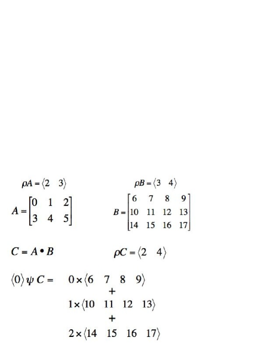
Data locality is maximized in that each row of the result (indicated by $<0>\psi C$ ) is computed at a time and the elements of $A$ and $B$ are accessed contiguously. In this figure we have illustrated some of the notational devices of MoA. In this formalism, the $\psi$ operator selects components and subarrays of a given array with the use of an index vector. In this case we select the zero’th row of $C$ with the operation $<0>\psi C$ . We see that each row of $B$ is multiplied by an element of $A$ and then added to the next row of $B$ multiplied by an element $A$ . This formulation of the inner product might seem simple but is actually quite subtle in the general case of two arbitrary multi-dimensional arrays. This way of organizing the operations leads to significant performance gains as will be demonstrated in the numerical tests to be described below.

In the rest of this paper we present performance tests of our routine for the computation of the standard matrix multiply in comparison with a benchmark routine (dgemm.f) taken from the BLAS library. We present tests of both sequential and OpenMP parallel implementations. We find that our routine is either competative or outperforms the BLAS routine.

As discussed more extensively below, our goal is to demonstrate the advantages of our design methodology using MoA. We don’t claim to have established the the best matrix multiply and in no way do we wish to enter such a competition. Indeed the matrix multiply has been extensively studied Dongarra et al. (1988a, b, 1990a, 1990b); Blackford et al. (2002); Whaley et al. (2001); Gunnels et al. (2001a, b); Gunnels et al. (2006); Geijn and Watts (1997); Low et al. (2005); Bientinesi et al. (2005a, b); Lawson et al. (1979a, b); Anderson et al. (1999) and we defer to the experts for those searching for the best matrix multiply. For our OpenMP version we also make no attempt at optimization. We simply adopt a “poor man’s” parallelism by wrapping sequential code with the simplest OpenMP statements (not even specifying a “chunk” size, for example). The point is that we take an “off the shelf” sequential benchmark, the standard BLAS routine dgemm.f and compare it with our generalized inner and outer product code for the limited case of matrix multiply and we find competative results without any optimizations other than the fortran compiler options $-O0$ , $-O1$ , $-O2$ and $-O3$ . For high performance parallel matrix multiply we again defer to the experts cited above as well as those in Refs. (Bentz and Kendal, 2005; Addison et al., 2003; Santos, 2003; Bilmes et al., 1997; Demmel et al., 2005; Bernsten, 1989; Choi et al., 1994; Huss-Lederman et al., 1993; Li, 2001; Irony et al., 2004).

II Numerical experiments

II.1 Computational Environment

A series of sequential and multi-processor tests were carried out for the MoA routine in comparison with the standard BLAS dgemm.f. The key code fragments are presented in the Appendix. A dedicated, non-shared, computational environment was used on the 5,120 processor machine “jaws” at the Maui High-Performance Computing Center. The following information is quoted from the website (www.mhpcc.hpc.mil):

“Jaws is a Dell PowerEdge 1955 blade server cluster comprised of 5,120 processors in 1,280 nodes. Each node contains 2 Dual Core 3.0 GHz 64-bit Woodcrest CPUs, 8GB of RAM, and 72GB of local SAS disk. Additionally, there is 200TB of shared disk available through the Lustre filesystem. The nodes are connected via Cisco Infiniband, running at 10Gbits/sec (peak). Jaws has a peak performance of 62400 GFlops, and LINPACK performance of 42390 GFlops.”

In the following we will present results for our new routine run in sequential and OpenMP multi-threaded tests.

II.2 Tests for matrix-matrix multiply

Our object of study is the computation of the matrix multiply $C=A*B$ where we consider $C$ to be a $m\times n$ matrix, where $m$ is the number of processors (threads) and $n$ is an integer power of $2$ and is varied from the smallest to largest sizes that can be accomodated. The matrix $A$ has dimensions $m\times\ell$ while $B$ has dimensions $\ell\times n$ . For these tests we keep $\ell$ fixed at the value $\ell=128$ .

There are two performance metrics of interest in this study: (1) the “time per thread” and (2) the “total time”. For a multi-thredded job the “time per thread” is simply the total time for the job to run. Note that a job with $m$ threads is dealing with a problem size that is $m$ times as large as the problem considered on $1$ thread. Thus if there were no communcation costs we would expect the curve of “time per thread” vs. $n$ to be the same, independent of the number of threads $m$ .

In some cases we wish to consider a fixed problem size and see how long it takes on $m=1$ , $2$ , $3$ , and $4$ processors. In this case we take the curves discussed in the previous paragraph and scale the $x$ axis (i.e. problem “size”) of each curve by multiplying by the corresponding number of processors $m$ . This type of plot should explicitly show the benefit of parallelism (if there is one) if the curve for $m$ threads is below that for $1$ thread.

II.3 Sequential tests

In a first series of numerical experiments we tested the MoA routine and the BLAS dgemm.f routine in sequential mode in a dedicated non-shared batch environment. Perl scripts were used in each case to compile the routine for a given value of $n$ and then the job is timed. This process is repeated three times for each $n$ and the timings were averaged. As reproducibility is a key concern, we also repeated several tests on different days of the week to make sure there were no substantial fluctuations. In all cases tested we found essentially identical results. From these careful considerations we conclude that all results presented in this work are reproducible.

Our initial interest was in determining the effect of compiler options on the performance of our routine and the BLAS routine. We thus ran our experiments with the four optimization flags: $-O0$ (no optimization), $-O1$ , $-O2$ and $-O3$ in four separate tests respectively. We used the Intel Fortran compiler “ifort” that was supplied with the machine. In all cases we found the compiler option $-O1$ to give the best performance. Thus in all results to be presented, we assume the compiler option $-O1$ to be in effect. Interestingly, for the MoA routine, we find a benefit on going from $-O0$ to $-O1$ but then no difference between $-O1$ , $-O2$ , and $-O3$ . In constrast, however, for the BLAS routine we find the speed to increase upon going from $-O0$ to $-O2$ and then to increase again upon going from $-O2$ to $-O1$ while the results for $-O2$ and $-O3$ were essentially identical.

Comparison of the MoA routine vs. the BLAS routine dgemm.f run in sequential mode are presented in Fig. 2. We see that the results are comparable with a slight benefit given by the MoA routine for small sizes. For the largest sizes that fit in real memory, the BLAS routine outperformes the MoA routine but for sizes requiring virtual memory the results are essentially the same. We will see that the superior performance of the BLAS routine at largest sizes is lost when we go to multiple threads using OpenMP.

II.4 Multiple-thread OpenMP

Our next set of computational experiments were performed using OpenMP multiple threads. On this machine (see description in first section) each node contains four processors (two dual cores) and so we restrict our attention in this series of experiments to $m=1$ , $2$ , $3$ , and $4$ threads. Making the transition from a sequential piece of code to open OpenMP is achieved by wraping the seqential algorithm, in each case with simple OpenMP directives. No attempt was made to optimize the parallel performance of either routine.

Our goal in the multi-threaded tests to be discussed herein is as follows. We are proceeding from a general, mathematically-based design methodology. Thus although our code was not designed to specifically exploit the multi-threading capabilities of this machine, we achieve impressive results in comparison with the BLAS benchmark. Again, we emphasize the design methodology. Our approach is completely mechanizable from the ONF (Operational Normal Form). That is given start, stop, stride, count, we can instantiate the software at any level of memory Hunt et al. ; Mullin and Raynolds (2008); Mullin (2005, 1991); Raynolds and Mullin (2005). We are not trying to claim that we have achieved the fastest multi-threaded matrix multiply. Nor are we comparing our results against a BLAS routine that has been designed for multi-processor, multi-threaded hardware. That is not our goal, but rather to argue the merits of a design methodology that consistently leads to efficient implementations by eliminating temporaries and exploiting data locality.

Figure 3 presents results for $m=1$ , $2$ , $3$ , and $4$ OpenMP threads for the MoA routine. We plot the time/thread for each job. In other words this is the total time for the job to run with the size of the problem proportional to the number of threads $m$ . This metric illustrates the communication cost associated with multiple threads because, in the absence of communication cost (i.e. in a situation of “perfect parallism”) the time/thread vs. $n$ (i.e. the number of columns of $C=AB$ ) would be independent of the number of threads $m$ .

In Fig. 4 we emphasize the net benefit of the use of multiple threads by considering the “total time” vs. the size of the problem. In other words, in this case, for each value of $m$ (i.e. the number of threads) we scale the $x$ -axis of the “time/thread” plot illustrated in Fig. 3 by $m$ . Thus for a given value of $n$ , if the curve for a given number of threads lies below that for $m=1$ , there is a net benefit to using multiple threads. We see that in this series of tests, there IS a net benefit to the use of $m=2$ threads but there is no net benefit for $m>2$ threads.

In Fig. 5 we plot the “time/thread” for the BLAS routine with $m=1$ , $2$ , $3$ and $4$ threads. The curves look similar to those for the MoA routine of Fig. 4 but as we will see the following figure there is a fundamental difference.

The results for the “total time” vs. $n$ for the BLAS routine are presented in Fig. 6. The results of Fig. 6, for the BLAS routine are fundamentally different from those for the MoA routine of Fig. 4 in that, while all the $m>1$ curves of Fig. 4 lie below the curve for $m=1$ , in Fig. 6 we see all $m>1$ curves lie above the $m=1$ result. Thus for this series of experiments there is no net benefit to the use of multiple threads for the BLAS routine.

In the next four figures we compare the “time/thread” for the MoA routine, directly with the BLAS routine. In Fig. 7 we compare the one-thread result for the MoA routine with the BLAS routine. We find that the MoA result out performs the BLAS routine for small matrix sizes and is equivalent to that of the BLAS routine for the largest sizes. Note that this figure should be directly compared with Fig. 2 for the sequential runs. We see that, although BLAS had the advantage for the largest sizes when running in sequential mode, the advantage is lost when going to $m=1$ thread using OpenMP.

For Figs. 8, through 10 we see that the MoA routine consistently out performs the BLAS routine for all sizes that fit into main memory. The BLAS routine out performs the MoA routine for sizes that only fit in virtual memory. The success of the MoA routine is due to the data locality of the algorithm’s contiguous access of all arguments: an output with two inputs.

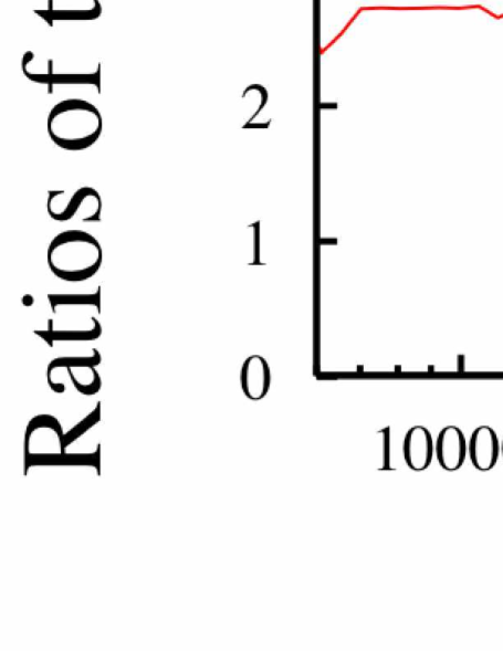
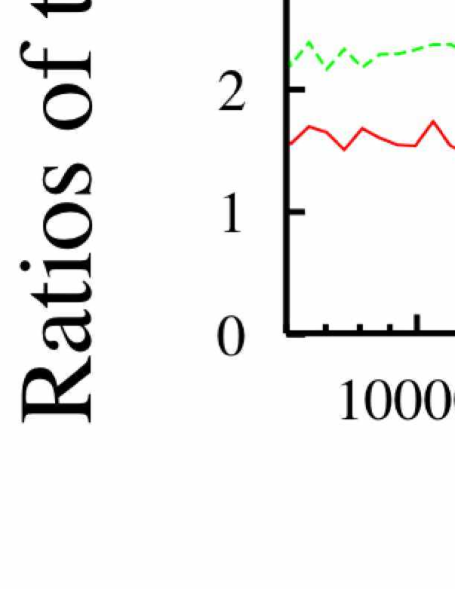
Another way to characterize the data we have considered so far is as follows. We consider the “time/processor” for each number of threads $m$ divided by the result for a single thread. Such results are presented in Figs. 11 and 12 for the BLAS routine and the MoA routine respectively. As argued previously, such a ratio should illustrate the effects of communication costs. If there were no communication cost, each ratio would be unity. Next, we consider the notion that if the ratio is greater than $m$ , there is no net benefit to using multiple threads as this would indicate that the job was more expensive than $m$ sequential jobs. For these (unoptimized) tests we conclude from Figs. 11 and 12 that there is no net benefit to the use of OpenMP multiple threads for the BLAS routine while there IS a net benefit to such use for the MoA routine.

Again, we emphasize that this result is not definitive for establishing a matrix multiply that is superior to BLAS. Indeed there are BLAS routines (and others) that are optimized for multiple threads and multiple processors Addison et al. (2003); Bentz and Kendal (2005); Santos (2003); Bernsten (1989); Chatterjee et al. ; Cherkassky and Smith (1988); Choi et al. (1994); Demmel et al. (1993); Fox et al. (1987); Huss-Lederman et al. (1993); Li (2001); Irony et al. (2004); Geijn and Watts (1997). We only emphasize the quality of our results as an advertisement for our methodical software design approach that exploits data locality as a fundamental principle.

III Conclusion

We have presented numerical tests of a generalized inner and outer product routine applicable to arbitrary multi-dimensional tensors specified at run time. Our algorithm computes either operation in a single piece of code. In this work we have focused on the limited case of matrix-matrix multiplication and have tested its performance for matrices from small sizes to the largest that can be possibly accomodated. As a benchmark reference we compare our results with the standard BLAS dgemm.f routine. We find that our routine is competative or out performs the BLAS routine. We have also presented tests of our routine using OpenMP parallelization without any machine specific optimizations (other than the compiler options $-O0$ , $-O1$ , $-O2$ and $-O3$ ). Again we find competative performance. As stated earlier, our goal is not to claim the best matrix multiply routine but rather to give definative tests of our routine for a well studied example: matrix multiply. Rather, we wish to emphasize the generality of our routine that can compute the inner and outer product between two arbitrary multi-dimensional arrays, as specified at run time, in a single piece of code.

Appendix A Code fragments for the numerical experiments

This appendix presents the key code fragments used in the testing of the BLAS routine (Fig. 13) and the MoA routine (Fig. 14)

c$OMP do private(i,j,l)
              DO 90 J = 1,N
                  IF (BETA.EQ.ZERO) THEN
                      DO 50 I = 1,M
                          C(I,J) = ZERO
   50                 CONTINUE
                  ELSE IF (BETA.NE.ONE) THEN
c  do 60 vectorized
                      DO 60 I = 1,M
                          C(I,J) = BETA*C(I,J)
   60                 CONTINUE
                  END IF
                  DO 80 L = 1,K
                      IF (B(L,J).NE.ZERO) THEN
                          TEMP = ALPHA*B(L,J)
c  do 70 vectorized
                          DO 70 I = 1,M
                              C(I,J) = C(I,J) + TEMP*A(I,L)
   70                     CONTINUE
                      END IF
   80             CONTINUE
   90         CONTINUE
c$OMP end do nowait

Figure 13: Key code fragment used in the benchmark tests of the BLAS routine. The first and last lines are the only OPenMP directives used in these tests and are the same as those used in the MoA tests.

c$OMP do private(k,i,l,j)
      do 100 k=0,(nthreads-1)
        do 120 i=k,(noproc-1),nthreads
          do 140 l=0,(rowsinred-1)
            do 160 j=0,(elsinop-1)
              RESADDR(1 + (i*restride) + j) =
     +              RESADDR(1 + (i*restride) + j) +
     +                 LADDR(1 + l + (i*lstride))*
     +                    RADDR(1 + (l*rstride) + j);
160         continue
140       continue
120     continue
100   continue
c$OMP end do nowait

Figure 14: Key code fragment used in the tests of the MoA routine. The first and last lines are the only OPenMP directives used in these tests and are the same as those used in the BLAS tests.

References

Mullin (1988) L. M. R. Mullin, Ph.D. thesis, Syracuse University (1988).
Dongarra et al. (1988a) J. J. Dongarra, J. D. Croz, S. Hammarling, and R. J. Hanson, ACM Trans. Math. Soft. 14, 1 (1988a).
Dongarra et al. (1988b) J. J. Dongarra, J. D. Croz, S. Hammarling, and R. J. Hanson, ACM Trans. Math. Soft. 14, 18 (1988b).
Dongarra et al. (1990a) J. J. Dongarra, J. D. Croz, S. Hammarling, and I. S. Duff, ACM Trans. Math. Soft. 16, 1 (1990a).
Dongarra et al. (1990b) J. J. Dongarra, J. D. Croz, I. S. Duff, and S. Hammarling, ACM Trans. Math. Soft. 16, 18 (1990b).
Blackford et al. (2002) L. S. Blackford, J. Demmel, J. Dongarra, I. Duff, S. Hammarling, G. Henry, M. Heroux, L. Kaufman, A. Lumsdain, A. Petitet, et al., ACM Trans. Math. Soft. 28, 135 (2002).
Whaley et al. (2001) R. C. Whaley, A. Petitet, and J. J. Dongarra, Parallel Computing 27, 3 (2001), also available as University of Tennessee LAPACK Working Note no. 147, UT-CS-00- 448, 2000 (http://www.netlib.org/lapack/lawns/lawn147.ps).
Gunnels et al. (2001a) J. A. Gunnels, G. M. Henry, and R. A. van de Geijn, in ICCS ’01: Proceedings of the International Conference on Computational Sciences-Part I (Springer-Verlag, London, UK, 2001a), pp. 51–60, ISBN 3-540-42232-3.
Gunnels et al. (2001b) J. Gunnels, F. Gustavson, G. Henry, and R. A. van de Geijn, Lecture Notes in Computer Science 2073, 51 (2001b).
Gunnels et al. (2006) J. Gunnels, F. Gustavson, G. Henry, and R. A. van de Geijn, Lecture Notes in Computer Science 3732, 256 (2006).
Geijn and Watts (1997) R. A. V. D. Geijn and J. Watts, Concurrencey: Practice and Experience 9, 255 (1997).
Low et al. (2005) T. M. Low, R. A. van de Geijn, and F. G. V. Zee, Proceedings of the Principles of Parallel Programming (POPP) p. 153 (2005).
Bientinesi et al. (2005a) P. Bientinesi, J. A. Gunnels, M. E. Myers, E. S. Quintana-Orti, and R. A. van de Geijn, ACM Transactions on Mathematical Software 31, 1 (2005a).
Bientinesi et al. (2005b) P. Bientinesi, E. S. Quintana-Orti, and R. A. van de Geijn, ACM Transactions on Mathematical Software 31, 27 (2005b).
Lawson et al. (1979a) C. L. Lawson, R. J. Hanson, D. Kincaid, and F. T. Krogh, ACM Trans. Math. Soft. 5, 308 (1979a).
Lawson et al. (1979b) C. L. Lawson, R. J. Hanson, D. Kincaid, and F. T. Krogh, ACM Trans. Math. Soft. 5, 324 (1979b).
Anderson et al. (1999) E. Anderson, Z. Bai, C. Bischof, S. Blackford, J. Demmel, J. Dongarra, J. D. Croz, A. Greenbaum, S. Hammarling, A. McKenney, et al., LAPACK User’s Guide. (SIAM, Philadelphia, PA, USA, 1999), third edition ed., also available in Japanese, published by Maruzen, Tokyo, translated by D. Oguni.
Bentz and Kendal (2005) J. L. Bentz and R. A. Kendal, Lecture Notes in Computer Science 3349, 1 (2005).
Addison et al. (2003) C. Addison, Y. Ren, and G. M. van Waveren, Scientific Programming 11, 95 (2003).
Santos (2003) E. E. Santos, J. Supercomp. 25, 155 (2003).
Bilmes et al. (1997) J. Bilmes, K. Asanovic, C. Chin, and J. Demmel, Proc. of Int. Conf. on Supercomputing, Vienna, Austria. (1997).
Demmel et al. (2005) J. Demmel, J. Dongarra, V. Eijkhout, E. Fuentes, A. Petitet, R. Vuduc, R. C. Whaley, and K. Yelick, Proceedings of the IEEE 93, 293 (2005).
Bernsten (1989) J. Bernsten, Parallel Computing 12, 335 (1989).
Choi et al. (1994) J. Choi, J. Dongarra, and D. W. Walker, Concurrency: Pract. & Exper. 6, 543 (1994).
Huss-Lederman et al. (1993) S. Huss-Lederman, E. M. Jacobson, and A. Tsao, in in Proceedings of the Scalable Parallel Libraries Conference, Starksville, MS (Society Press, 1993), pp. 142–149.
Li (2001) K. Li, Journal of Parallel and Distributed Computing 61, 1709 (2001).
Irony et al. (2004) D. Irony, S. Toldedo, and A. Tiskin, Journal of Parallel and Distributed Computing 64, 1017 (2004).
(28) H. B. Hunt, L. R. Mullin, D. J. Rosenkrantz, and J. E. Raynolds, A transformation–based approach for the design of parallel/distributed scientific software: the FFT, (arXiv:0811.2535, 2008).
Mullin and Raynolds (2008) L. R. Mullin and J. E. Raynolds, Conformal Computing: Algebraically connecting the hardware/software boundary using a uniform approach to high-performance computation for software and hardware applications (arXiv:0803.2386, 2008).
Mullin (2005) L. R. Mullin, Digital Signal Processing 15, 466 (2005).
Mullin (1991) L. R. Mullin, in Arrays, Functional Languages, and Parallel Systems (Kluwer Academic Publishers, 1991).
Raynolds and Mullin (2005) J. E. Raynolds and L. R. Mullin, Comp. Phys. Comm. 170, 1 (2005).
(33) S. Chatterjee, A. Lebeck, P. Patnala, and M. Thottethodi, Recursive array layouts and fast parallel matrix multiplication, in Proceedings of the Symposium on Parallel Algorithms and Architecture.
Cherkassky and Smith (1988) V. Cherkassky and R. Smith, J. Supercomputing 2, 7 (1988).
Demmel et al. (1993) J. W. Demmel, M. T. Heath, and H. A. van der Vorst, Tech. Rep. UCB/CSD 93/703, University of California at Berkeley, Berkeley, CA, USA (1993).
Fox et al. (1987) G. Fox, S. Otto, and A. Hey, Parallel Computing 4, 17 (1987).