A Generative Model of Symmetry Transformations
Abstract
Correctly capturing the symmetry transformations of data can lead to efficient models with strong generalization capabilities, though methods incorporating symmetries often require prior knowledge. While recent advancements have been made in learning those symmetries directly from the dataset, most of this work has focused on the discriminative setting. In this paper, we take inspiration from group theoretic ideas to construct a generative model that explicitly aims to capture the data’s approximate symmetries. This results in a model that, given a prespecified but broad set of possible symmetries, learns to what extent, if at all, those symmetries are actually present. Our model can be seen as a generative process for data augmentation. We provide a simple algorithm for learning our generative model and empirically demonstrate its ability to capture symmetries under affine and color transformations, in an interpretable way. Combining our symmetry model with standard generative models results in higher marginal test-log-likelihoods and improved data efficiency.
1 Introduction
Many physical phenomena exhibit symmetries; for example, many of the observable galaxies in the night sky share similar characteristics when accounting for their different rotations, velocities, and sizes. Hence, if we are to represent the world with generative models, they can be made more faithful and data-efficient by incorporating notions of symmetry. This has been well-understood for discriminative models for decades. Incorporating inductive biases such as invariance or equivariance to symmetry transformations dates back (at least) to ConvNets, which incorporate translation symmetries (LeCun et al., 1989)—and can be extended to reflection and rotation (Cohen and Welling, 2016)—and more recently, transformers, with permutation symmetries (Lee et al., 2019).
In many cases, it is not known a priori which symmetries are present in the data. Learning symmetries in discriminative modeling is an active field of research (Nalisnick and Smyth, 2018; van der Wilk et al., 2018; Benton et al., 2020; Schwöbel et al., 2021; van der Ouderaa and van der Wilk, 2022; Rommel et al., 2022; Romero and Lohit, 2022; Immer et al., 2022, 2023; Miao et al., 2023; Mlodozeniec et al., 2023). However, in these works—which focus on invariant discriminative models—the label is often assumed to be invariant, and thus, the symmetry information can be removed rather than explicitly modeled. On the other hand, a generative model must capture the factors of variation corresponding to the symmetry transformations of the data. Doing so can provide benefits such as better representation learning—by disentangling symmetry from other latent variables (Antorán and Miguel, 2019)—and data efficiency—due to compactly encoding of factor(s) of variation corresponding to symmetries. Furthermore, learning about underlying symmetries in data could be used for scientific discovery.
We propose a generative model that explicitly encodes the (approximate) symmetries in the data. Here, we are primarily interested in using this model to inspect the distribution over naturally occurring transformations for a given example , and resample new “naturally” augmented versions of the example. Our contributions are
-
1.
We propose a Symmetry-aware Generative Model (SGM). The SGM’s latent representation is separated into an invariant component and an equivariant component . The latter, , captures the symmetries in the data, while captures none. We recover by applying a parameterised transformation, . We call a prototype since each can produce arbitrarily transformed observations; see Figure˜1.
-
2.
We propose a two-stage algorithm for learning our SGM: first learning using a self-supervised approach and then learning via maximum likelihood. Importantly, this does not require modeling the distribution of prototypes , allowing the procedure to remain tractable even for complex data.
-
3.
We verify experimentally that our SGM correctly captures affine and color symmetries. A VAE’s marginal test-log-likelihood can be improved by using our SGM to incorporate symmetries. Additionally, unlike a standard VAE, explicitly modeling symmetries makes our VAE-SGM hybrid robust to the removal of three quarters of the training data.
Notation.
We use , , and (i.e., lower, bold lower, and bold upper case) for scalars, vectors, and matrices, respectively. We distinguish between random variables such as , , , and their realizations , , , by italicizing the realizations. Thus, for continuous , is a PDF that returns a density . We use to represent function composition, e.g., .
2 Symmetry-aware Generative Model (SGM)
Consider a dataset of observations on a space , and a collection of transformations parameterised by transformation parameters . We assume (abbreviated ) form a group. Loosely, our aim is to model the distribution over transformations present in the data. To do so, we model the distribution by decomposing it into two disparate parts: (1) a distribution over prototypes and (2) a distribution over parameters controlling transformations to be applied to a prototype. Concretely, we specify our generative model as follows (also depicted in Figure˜2):
| (1) | ||||
| (2) | ||||
| (3) |
That is, the SGM assumes that each observation is generated by applying a transformation —parameterized by a latent variable —to a latent prototype . Since , by assumption, contains no information about the symmetries in the data, must model the distribution over the transformations present in the data.
Motivation.
Why would we expect specifying in this way to be useful? Firstly, our SGM allows us to query a distribution over naturally occurring transformations for any input , given the matching prototype . Secondly, we expect our SGM to align with the true physical process of generating the data for many interesting datasets. As an illustrative example, when a person writes a digit, they first decide what kind of digit to write—e.g., the prototype could be an upright ‘3’—but when they put pen to paper, the digit they pictured is transformed due to various factors governing their handwriting111Our SGM does not always perfectly match the data-generating process. E.g., a person is unlikely to “imagine” the same prototype for both a ‘6’ or a ‘9’—which can often be transformed into one another with rotation.. Similarly, when a photographer captures an object, the photo is also a function of latent factors of variation, such as lighting, the lens, camera shake, etc.
What do we require of a prototype?
can informally be considered a canonical/reference example with no transformation applied to it. More precisely, we require that for any orbit of an element —defined as the set of elements in which can be mapped to by a transformation in —there is exactly one prototype in the orbit. Figure˜1 depicts an example orbit—a set of all rotated variants of a ‘3’—with a unique prototype.
Why do we want a group?
Having the transformations be a group simplifies things, since will then naturally partition the space into (disjoint) orbits. Within each orbit, every element can be transformed into one another with a transformation in . As an example of such a partition, if our collection of transformations were horizontal shifts acting on a point , then the different orbits will correspond to all points on a given horizontal line; see Figure˜3. Therefore, if we have chosen a unique prototype for each orbit and forms a group, any two elements will have the same prototype if and only if they can be transformed into one another.
In Section˜2.1, we describe a method for learning a transformation inference function , with parameters , that for returns transformation parameters as . These map to a prototype that generates 222The transformation is not necessarily unique.. We then apply standard generative modeling tools to learn given the generated data pairs .
2.1 Learning
We now discuss learning for the two NNs required by our model, and . In Appendix˜A, we connect our learning algorithm with MLL optimization using an ELBO.
Transformation inference function.
For , with given by , to map to a prototype , it must, by definition, map all elements in any given orbit to the same element in that orbit. In other words, the output of should be invariant to transformations of :
| (4) |
To learn such a function, we optimize for this property directly. To this end, we sample transformation parameters from some distribution over parameters . This allows us to get random samples in the orbit of any given element . Since we want full (i.e., strict) invariance, must have support on the entire orbit (van der Ouderaa and van der Wilk, 2022). We then learn an equivariant function 333 If is equivariant by construction, our SSL scheme is unnecessary. Alas, such constructions are unknown for many transformations, like those in this paper. Thus, we provide a general method for learning equivariances. via a self-supervised learning (SSL) scheme inspired by methods like BYOL (Grill et al., 2020) and, more directly, BINCE (Dubois et al., 2021). For example, we could use the objective illustrated in Figure˜4:
| (5) |
Our actual objective differs slightly. Since implies , we use
| (6) |
This change allows us to reduce the number of small discretization errors introduced with each transformation application by replacing repeated transformations with a single composed transformation; see Section˜3.1 for further discussion. Our SSL loss is given in Algorithm˜1 of Algorithm˜1.
Generative model of transformations.
Once we have a prototype inference function, we simply learn by maximum likelihood on the created data pairs . This is shown in ˜6 of Algorithm˜1. While we need to specify the kinds of symmetry transformations we expect to see in the data, by learning the model can learn the degree to which those transformations are present in the data. Thus, we can specify several potential symmetry transformations and learn that some are absent in the data. Furthermore, the required prior knowledge (the support of ) is small compared to what our SGM can learn (the shapes of the distributions for each of the present transformations).
Since we are primarily interested in using the model to (a) inspect the distribution over naturally occurring transformations for a given element , and (b) resample new “naturally” augmented versions of the element, we do not need to learn . We can do (a) by querying for , and we can do (b) by sampling and transforming to get . Of course, if one wanted to sample new prototypes, one could fit using, e.g., a VAE. Not learning greatly simplifies training for complicated datasets that would otherwise require a large generative model, an observation made by Dubois et al. (2021).
3 Practical Considerations and Further Motivations
Training our SGM, while simple, has potential pitfalls in practice. We discuss the key considerations in Section˜3.1 and provide further recommendations in Appendix˜B. We then provide motivation for several of our modeling choices in Section˜3.2.
3.1 Practical Considerations
Working with transformations.
Repeated application of transformations—e.g., in Figure˜4—can introduce unwanted artifacts such as blurring. For many useful transformations, we can compose transformations before applying them. For affine transformations of images, for example, we can directly multiply affine-transformation matrices. More generally, if there is some representation of the transformation parameters where composition can be performed—e.g., as matrix multiplication , in the case where is a group representation—then we recommend composing transformations in that space to minimize the number of applications.
Partial invertibility.
In many common settings, transformations are not fully invertible. We encounter two such issues when working with affine transformations of images living in a finite, discrete coordinate space. Firstly, affine transformations are only approximately invertible in the discrete space due to the information loss when interpolating the transformed image onto a discrete grid. Thus, while only a single prototype exists for any , it may not be clear what the correct prototype is. Secondly, transformations can cause information loss due to the finite coordinate space (e.g., by shifting the contents of the image out-of-bounds444 This can occur in practice since our SSL objective—which aims to make prototypes as similar as possible—can trivially be minimized by removing all of the contents of an image. ). If appropriate bounds are known a priori, we can prevent severe information loss by constraining and using , , and bijectors. Alternatively, we can augment the SSL loss in Algorithm˜1 with an invertibility loss
| (7) |
Learning with imperfect inference.
In practice, our transformation inference network will not be perfect; see Figure˜10. Even after training, there may be small variations in the prototypes corresponding to different elements in the orbit of . To make robust to these variations, we train it with prototypes corresponding to randomly transformed training data points. I.e., we modify the MLE objective in Algorithm˜1 as , where as in our SSL objective. Averaging the loss over multiple samples—e.g., 5—of is beneficial.
|
8 |
8 | |
|
8 |
8 | |
|
8 |
8 |
3.2 Modelling Choices
We now motivate some of the design choices for our SGM by means of illustrative examples. In each case, we assume that is counter-clockwise rotation; thus, is the angle.
1. The distribution is implemented as a normalizing flow.
Consider a dataset of ‘8’s rotated in the range to : { 8 , …, 8 , …, 8 }. Let us assume that the prototype is ‘8’. Figure˜5(a) shows , an example of the true distribution for given and , for several observations, under the data generating process555 Because ‘8’ is symmetric, could be any convex combination of the two delta distributions. However, for a more realistic example, consider a prototype ‘8’ with a smaller upper loop. In this case, the must be bimodal to capture ‘8’s with both smaller upper and lower loops. . These distributions are composed of deltas because only certain values of will transform into . Figures˜5(b) and 5(c) compare idealised examples of the learned —given a simple uni-modal Gaussian family and a more flexible bi-modal mixture-of-Gaussian family—with the aggregate true distribution . Here, the simple uni-modal distribution is clearly worse than the bi-modal distribution due to the large amount of probability mass being wasted on angles with low density under the true data-generating process. Of course, one might argue that the bi-modal distribution is also not flexible enough. Furthermore, ‘flexible enough’ will be problem-specific. We solve this problem by modeling with normalizing flows, which can match a wide range of distributions.
|
2 |
2 | |
|
2 |
2 | |
|
2 |
2 | |
|
8 |
8 | |
|
8 |
8 | |
|
8 |
8 |
2. The transformation parameters depend on the prototype .
Consider a dataset of ‘2’s and ‘8’s rotated in the range to : { 2 , …, 2 , …, 2 , 8 , …, 8 , …, 8 }, with prototypes ‘2’ and ‘8’. Figure˜6(a) shows , an example of a true distribution over , for several observations. Figures˜6(b) and 6(c) compare idealized examples of learned distributions over and . Without dependence on , the model must place probability mass between and , in order to capture the symmetries of the ‘8’s, however this results invalid digits—such as { 2 , 2 , 2 }—which do not come from true data distribution. On the other hand, when depends on , the distribution conditioned on the prototype for the ‘2’s only needs to place mass in .
| (a) Full | (b) Partial | (c) None | ||||
|---|---|---|---|---|---|---|
|
2 |
2 |
2 |
2 |
|||
|
2 |
2 |
2 |
2 |
|||
|
2 |
2 |
2 |
2 |
|||
3. The prototype is fully invariant to transformations of .
Models such as CNNs are most useful when we know a priori which symmetries are present in the data. However, in many cases, this must be learned. In the case of handwritten digit recognition, we know that the model should be invariant to some amount of rotation since people naturally write with some variation in angle. But a model that is invariant to rotations in the full range might be unable to distinguish between ‘6’ and ‘9’. Thus, in the literature for learning invariances in the discriminative setting, it is common to learn partially invariant functions that capture some degree of invariance (van der Wilk et al., 2018; Benton et al., 2020; van der Ouderaa and van der Wilk, 2022). However, as we will now show, this approach is unsuitable for our SGM, as it breaks our assumption that contains no information about the symmetries in the data.
Consider a dataset of ‘2’s rotated in the range to : { 2 , …, 2 , …, 2 }. Figure˜7(a) shows predicted prototypes and the corresponding distributions over for several observations. There are three cases: (a) a fully-invariant , i.e., there is a single prototype, (b) a partially-invariant , for which there are two prototypes in this example, and (c) a non-invariant , which takes the partially-invariant case to the extreme and has as many prototypes as observations. In the partially-invariant and non-invariant cases, we can get multiple prototypes rather than a single unique prototype per orbit, which is invalid under the generative model of the data. As a result, does not represent the distribution of naturally occurring transformations of in the data. This is illustrated in Figures˜7(b), 7(c) and 7(d), which show idealized examples of the learned in each case. While the distribution in Figure˜7(b) matches the distribution of transformations in the dataset, in Figures˜7(c) and 7(d) we see that the distributions corresponding to non-unique prototype do not.
To illustrate why this is a problem, let us say we would like to probe the probability of a particular transformed variant of an observed example. For example, given an example of a digit ‘3’, we want to know the probability of observing , that digit rotated by . Assuming we can find a prototype , we would like to represent all naturally occurring augmentations. Unless is unique, this won’t necessarily be the case, as shown in Figures˜7(c) and 7(d).
4 Experiments
In Section˜4.1, we explore our SGM’s ability to learn symmetries. We show that it produces valid prototypes, and generates plausible samples from the data distribution, given those prototypes. Then, in Section˜4.2, we leverage our SGM to improve data efficiency in deep generative models.
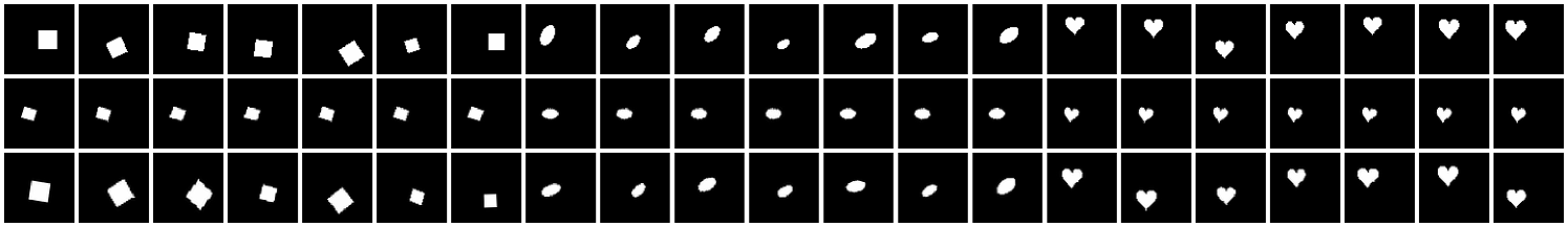
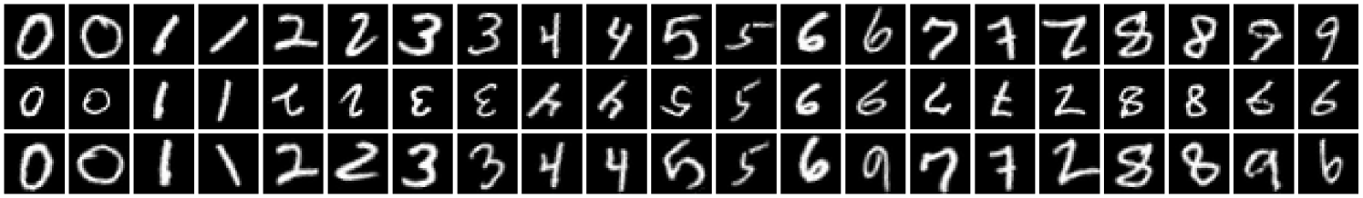
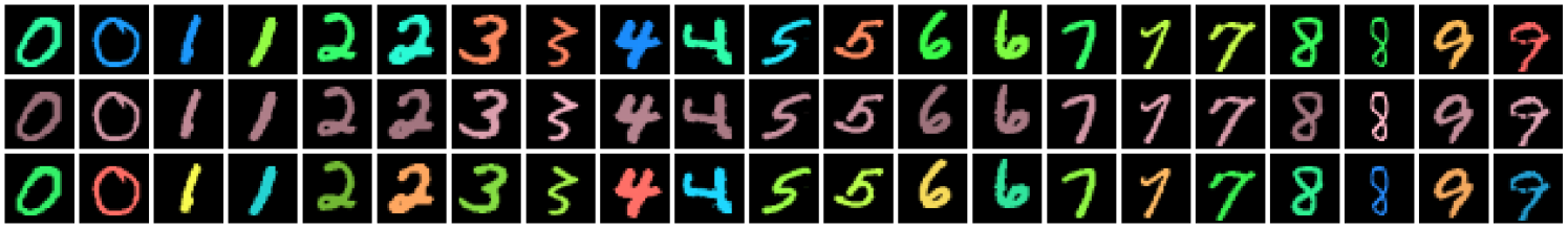
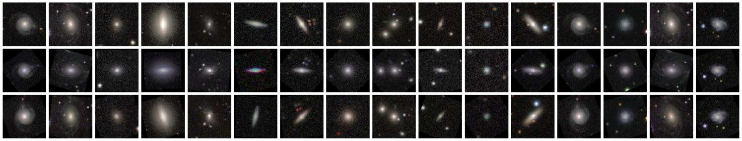
Here, we conduct experiments using three datasets—dSprites (Matthey et al., 2017), MNIST, and GalaxyMNIST (Walmsley et al., 2022)—and two kinds of transformations—affine and color. Results for PatchCamelyon (Veeling et al., 2018) are in Section˜E.2. In Section˜4.1, when working with MNIST under affine transformations, we add a small amount of rotation (in the range) to the original data to make rotations in the figures easier to see. For MNIST under color transformations, we first convert the grey-scale images to color images using only the red channel. We then add a random hue rotation in the range and a random saturation multiplier in the range . In the case of dSprites, we carefully control the rotations, positions, and sizes of all of the sprites. For example, in the case of the heart sprites, we have removed the rotations and set the -positions to be bimodal in the top and bottom of the images. We focus on learning affine transformations (shifting, rotation, and scaling) as they are expressive but easy to work with, as well as color transformations (hue, saturation, and value). Details about our experimental setup—including hyperparameter sweeps, our modified dSprites dataset, and parameterizations for —can be found in Appendix˜C.
4.1 Learning Symmetries
Exploring transformations and prototypes.
Figure˜8 shows that for both datasets and kinds of transformations we consider, our SGM produces close-to-invariant prototypes as well as realistic “natural” examples that are almost indistinguishable from test examples. There are several illustrative examples which warrant further discussion. The heart sprites in Figure˜8(a) show that our SGM was able to learn the absence of a transformation (namely rotation) in the dataset.
As expected, all of the prototypes for the sprites of the same shape are the same, since these shapes are in the same orbit as one another. This behaviour is also demonstrated for MNIST digits in Figures˜19 and 20. The ‘6’, ‘8’, and ‘9’ digits in Figure˜8(b) demonstrate the ability of our SGM to learn bimodal distributions (on rotation in this case). The figure’s third ‘7’ is interesting because our SGM interprets it as a ‘2’.
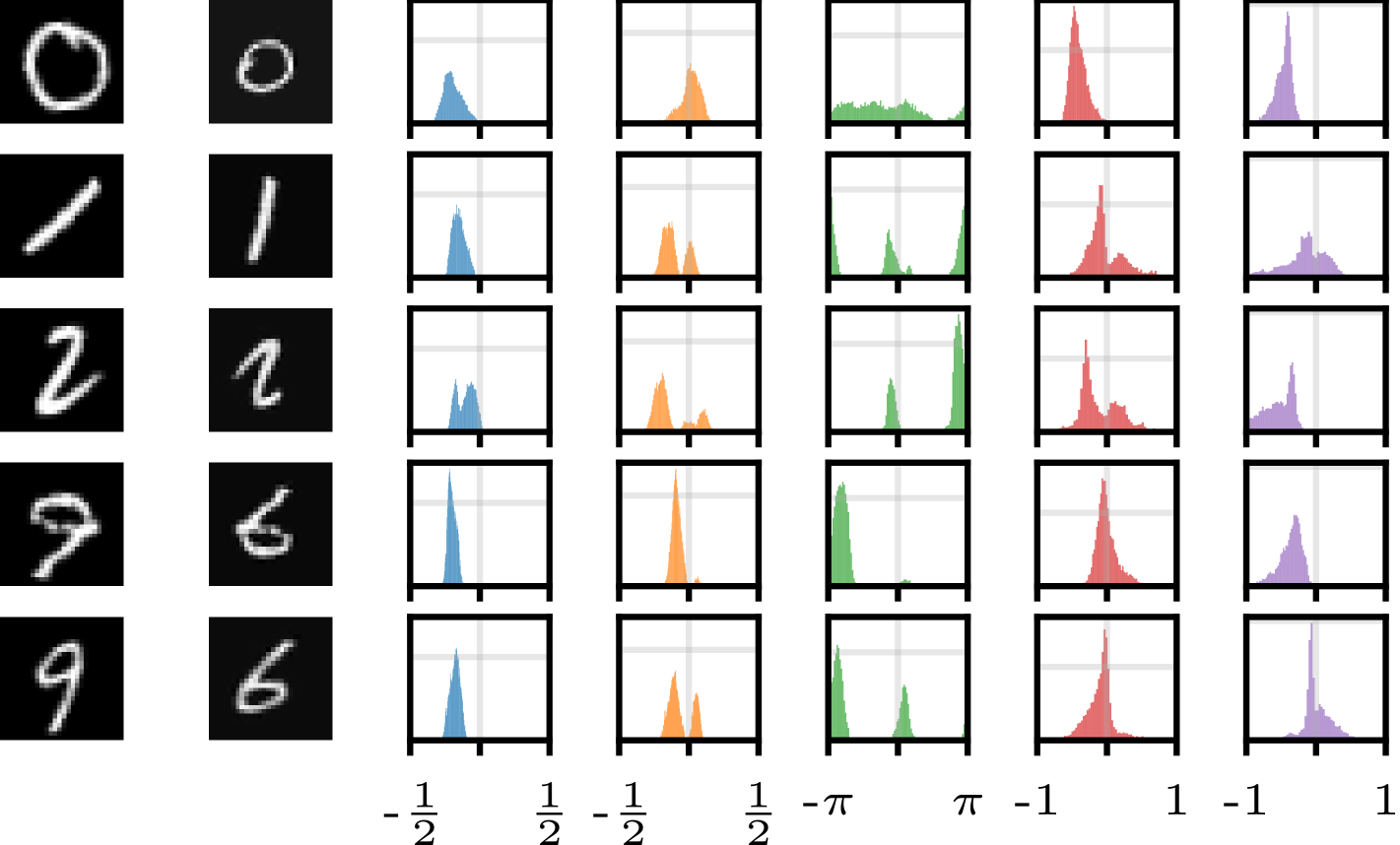
Flexibility is important.
In , each dimension corresponds to a different transformation. We refer to as the marginal distribution of a single transformation parameter. Figure˜9 shows the learnt marginal distributions for several digits from Figure˜8(b). We see that each of the parameters has its own range and shape. For rotations, which are easy to reason about, we see distributions that make sense—the round ‘0’ has an almost uniform distribution over rotations, and the ‘1’ and one of the ‘9’s are strongly bimodal as expected. The other ‘9’, which does not look as much like an upside-down ‘6’, has a much smaller mode. The ‘2’, which looks somewhat like an upside-down ‘7’, is also bimodal. We see that prototypes of different sizes result in corresponding distributions over scaling parameters with different ranges. Figure˜21 provides additional examples for MNIST with affine transformations, while Figure˜22 provides the same for color transformations, and Figure˜23 investigates the distributions for dSprites. These results provide experimental evidence of the need for flexibility in the generative model for , as conjectured in Section˜3.2. We also find significant dependencies between dimensions of (e.g., rotation and translation in dSprites).
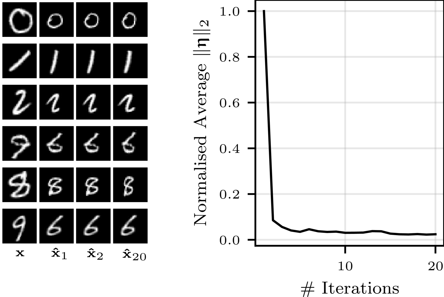
Invariance of and the prototypes.
In Figure˜10, we investigate the imperfections of the inference network by considering an iterative procedure in which prototypes are treated as observed examples, allowing us to infer a chain of successive prototypes. We show several examples of such chains, as well as the average magnitude of the transformation parameters at each iteration, normalized by the maximum magnitude (at iteration 0). The first prototype is most different from the previous , with successive prototypes being similar visually and as measured by the magnitude of the inferred transformation parameters. However, the magnitude of the inferred parameters does not tend towards 0, rather plateauing at around 5% of the maximum. This highlights that, although simple NNs can learn to be approximately invariant, a natively invariant architecture has the potential to improve performance.
4.2 VAE Data Efficiency
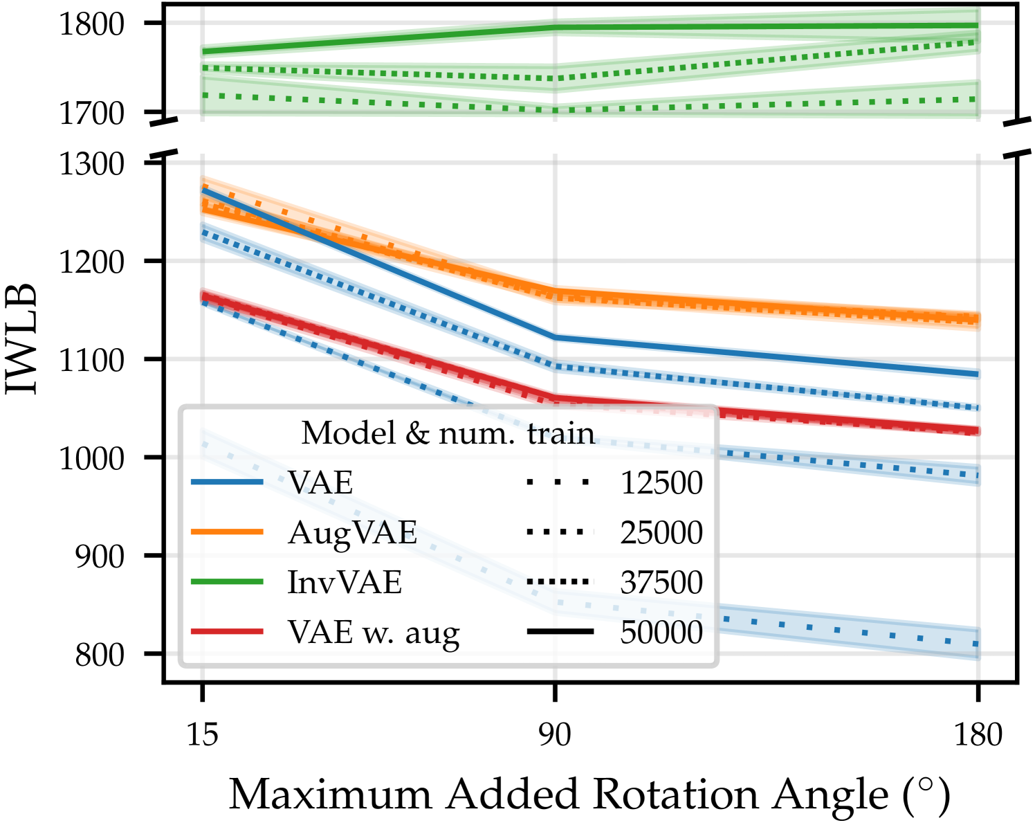
We use our SGM to build data-efficient and robust generative models. In Figure˜11, we compare a standard VAE to two VAE-SGM hybrid models—“AugVAE” and “InvVAE”—for different amounts of training data and added rotation of the MNIST digits. When adding rotation, each in the dataset set is always rotated by the same angle (sampled uniformly between , the maximum added rotation angle). Thus, adding rotation here is not data augmentation. AugVAE is a VAE that uses our SGM to re-sample transformed examples , introducing data augmentation at training time. InvVAE is a VAE that uses our SGM to convert each example to its prototype at both train and test time. That is, the VAE in InvVAE sees only the invariant representation of each example. We also compare against a VAE trained with standard data augmentation666 We use , zoom , and x/y-shift . . We use test-set importance-weighted lower bound (IWLB) (Domke and Sheldon, 2018) of , estimated with 300 samples of the VAE’s latent variable , and for InvVAE, to compare the models. Reconstruction error is provided in Appendix˜E. Further details—e.g., hyperparameter sweeps—are in Appendix˜C.
As expected, for the VAE ( ), as we decrease the amount of training data ( ) or increase the amount of randomly added rotation, performance degrades. This is because the VAE sees fewer training examples per-degree of rotation. On the other hand, the AugVAE ( ) is more data efficient. Its performance is unaffected by reducing the number of observations by three quarters. Furthermore, while the performance of AugVAE and the standard VAE are almost identical for small angles and large training sets, the drop in performance of AugVAE for larger random rotations is significantly smaller; AugVAE does not see less training examples per-degree of rotation. InvVAE ( ), which natively incorporates the inductive biases of our SGM, obtains a 500 nat larger likelihood than the other models. Its performance is almost perfectly robust to rotation in the dataset. Additionally, its metrics barely change () when trained on half the data. Finally, while the VAE with data augmentation ( ) improves on the standard VAE for less training data, it is substantially worse in the presence of more data. This contrasts our AugVAE, which is almost always better. This poor performance is because the augmentations are independent of the samples. Thus, highly rotated digits can be rotated too much, smaller digits become too small, and digits near the image edges are moved out of frame. This highlights the importance of augmenting data in accordance with the true data distribution.
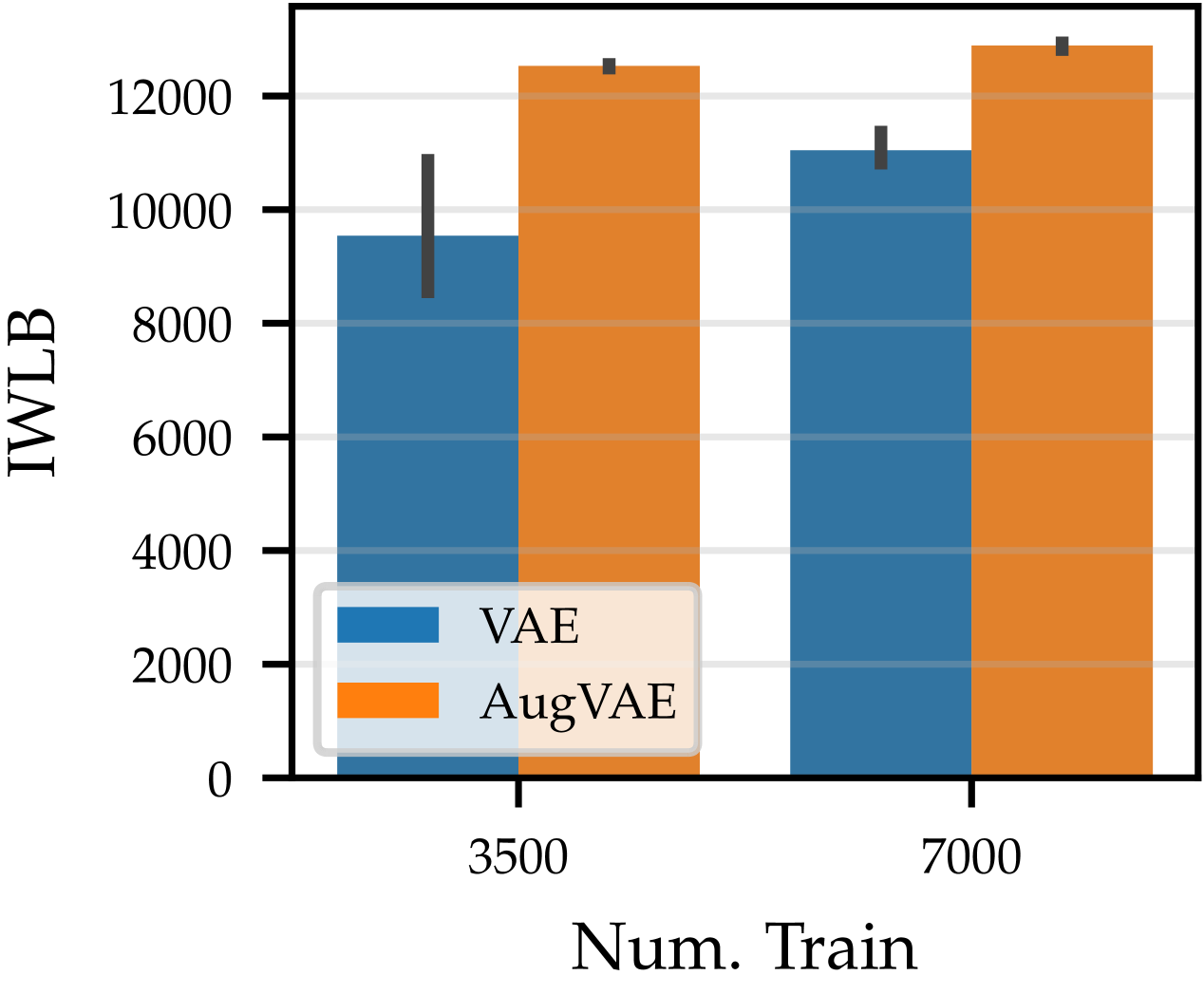
We further validate these results with the more complex GalaxyMNIST dataset and an enlarged set of both affine and color transformations. As with our rotated MNIST with affine transformation results, in Figure˜12, we see that AugVAE ( ) outperforms the standard VAE ( ). Furthermore, we see that AugVAE is robust to training with only half of the dataset. Our SGM captures the true data distribution with only 3500 training examples.
5 Related Work
Learning Lie groups.
Rao and Ruderman (1998); Miao and Rao (2007); Keurti et al. (2023) learn Lie groups from sequences of transformed images in an unsupervised fashion. Hashimoto et al. (2017) learn to represent an image as a linear combination of transformed versions of its nearest neighbors. Dehmamy et al. (2021) use Lie algebras to define CNNs for automatic symmetry discovery. Yang et al. (2023) use a GAN-based approach to learn transformations of examples that leave the original data distribution unchanged, thereby fooling a discriminator. Falorsi et al. (2019) introduce a reparameterization trick for learning densities on arbitrary, but known, Lie groups. Chau et al. (2022) learn a generative model over Lie group transformations applied to prototypical images that are themselves composed of sparse combinations of learned dictionary elements.
Learning a prototype.
Kaba et al. (2023) note that symmetry-based NNs are often constrained in their architectures. Like us, they propose to learn "canonicalization functions" that produce prototypical representations of the data. Mondal et al. (2023) show that such canonicalization functions can be used to make large-pre-trained NNs equivariant and, when combined with dataset-dependent symmetry priors, do not degrade performance. Similarly, Kim et al. (2023) learn architecture-agnostic equivariant functions by averaging a non-equivariant function over a probabilistic prototypical input. Finally, while not explicitly trained to produce prototypes, spatial transformer networks learn to undo transformations such as translation, scaling, and rotations (Jaderberg et al., 2015).
Data augmentations and symmetries.
Prior work makes several connections between data augmentation and symmetries relevant to our findings. Bouchacourt et al. (2021b) show that invariances in the model tend to result from natural variations in the data rather than data augmentation or model architecture. This supports our approach of learning data augmentation from the data and our architecture-agnostic self-supervised invariance learning method. Balestriero et al. (2022); Miao et al. (2023); Bouchacourt et al. (2021b) show that learned symmetries (i.e., data augmentation) should be class-dependent, much like our transformations are prototype-dependent.
Symmetry-aware latent spaces.
Encoding symmetries in latent space is well-studied. Higgins et al. (2018) posit that symmetry transformations that leave some parts of the world invariant are responsible for exploitable structure in any dataset. Thus, agents benefit from disentangled representations that separate out these transformations. Winter et al. (2022) split the latent space of an auto-encoder into invariant and equivariant partitions. However, they rely on in- and equivariant NN architectures, contrasting with our self-supervised learning approach. Furthermore, they do not learn a generative model—they reconstruct the input exactly—thus, they cannot sample new observations given a prototype. Xu et al. (2021) propose group equivariant subsampling layers that allow them to construct autoencoders with equivariant representations. Shu et al. (2018) propose an autoencoder whose representations are split such that the reconstruction of an observation is decomposed into a “template” (much like our prototypes) and a spatial deformation (transformation).
In the generative setting, Louizos et al. (2016) construct a VAE with a latent space that is invariant to pre-specified sensitive attributes of the data. However, these sensitive attributes are observed rather than learned. Similarly, Aliee et al. (2023) construct a VAE with a partitioned latent space with a component that is invariance spurious factors of variation in the data. Bouchacourt et al. (2018); Hosoya (2019) learn VAE with two latent spaces—a per-observation equivariant latent and an invariant latent shared across grouped examples. Other works have constructed rotation equivariant (Kuzina et al., 2022) and partitioned equivariant and invariant (Vadgama et al., 2022) latent spaces. Antorán and Miguel (2019); Ilse et al. (2020) split the latent space of a VAE into domain, class, and residual variation components. The first of which can capture rotation symmetry in hand-written digits. Unlike us, they require class labels and auxiliary classifiers. Keller and Welling (2021) construct a VAE with a topographically organized latent space such that an approximate equivariance is learned from sequences of observations. In contrast to the works above, Bouchacourt et al. (2021a) argue that learning symmetries should not be achieved via a partitioned latent space but rather learning equivariant operators that are applied to the whole latent space. Finally, while Nalisnick and Smyth (2017) do not learn symmetries, their information lower bound objective is reminiscent of several works above—and our own, see Appendix˜A—in minimizing the mutual information between two quantities when learning a prior.
Self-supervised Equivariant Learning
(Dangovski et al., 2022) generalize standard invariant SSL methods to produce representations that can be either insensitive (invariant) or sensitive (equivariant) to transformations in the data. Similarly, Eastwood et al. (2023) use a self-supervised learning approach to disentangle sources of variation in a dataset, thereby learning a representation that is equivariant to each of the sources while invariant to all others.
6 Conclusion
We have presented a Symmetry-aware Generative Model (SGM) and demonstrated that it is able to learn, in an unsupervised manner, a distribution over symmetries present in a dataset. This is done by modeling the observations as a random transformation of an invariant latent prototype. This is the first such model we are aware of. Building generative models that incorporate this understanding of symmetries significantly improves log-likelihoods and robustness to data sparsity. This is exciting in the context of modern generative models, which come increasingly close to exhausting all of the data on the internet. We are also excited about the use of SGM for scientific discovery, given that the framework is ideal for probing for naturally occurring symmetries present in systems. For example, we could apply SGM to marginalize out the idiosyncrasies of different measuring equipment and observation geometry in radio astronomy data. Additionally, given the success of using our SGM for data augmentation when training VAEs, it would be interesting to apply it to data augmentation in discriminative settings and compare it with methods such as Benton et al. (2020); Miao et al. (2023).
The main limitation of our SGM is that it requires specifying the super-set of possible symmetries. Future work might relax this requirement or explore how robust our SGM is to even larger sets. Furthermore, care must sometimes be taken when specifying the set of symmetries. For example, when rotating images with “content” at the boundaries of the image; see Section˜E.2.
Acknowledgements
The authors would like to thank Taliesin Beynon for helpful discussions and Emile Mathieu for providing feedback on the paper. This work has been performed using resources provided by the Cambridge Tier-2 system operated by the University of Cambridge Research Computing Service (http://www.hpc.cam.ac.uk) funded by EPSRC Tier-2 capital grant EP/T022159/1. This work was also supported with Cloud TPUs from Google’s TPU Research Cloud (TRC). JUA acknowledges funding from the EPSRC, the Michael E. Fisher Studentship in Machine Learning, and the Qualcomm Innovation Fellowship. JUA was also supported by an ELLIS mobility grant. SP acknowledges support from the Harding Distinguished Postgraduate Scholars Programme Leverage Scheme. JA acknowledges support from Microsoft Research, through its PhD Scholarship Programme, and from the EPSRC. JMH acknowledges support from a Turing AI Fellowship under grant EP/V023756/1. RET is supported by Google, Amazon, ARM, Improbable, EPSRC grant EP/T005386/1, and the EPSRC Probabilistic AI Hub (ProbAI, EP/Y028783/1).
References
- Aliee et al. (2023) Hananeh Aliee, Ferdinand Kapl, Soroor Hediyeh-Zadeh, and Fabian J. Theis. Conditionally invariant representation learning for disentangling cellular heterogeneity. CoRR, abs/2307.00558, 2023. doi: 10.48550/arXiv.2307.00558.
- Allingham et al. (2022) James Urquhart Allingham, Javier Antoran, Shreyas Padhy, Eric Nalisnick, and José Miguel Hernández-Lobato. Learning generative models with invariance to symmetries. In NeurIPS 2022 Workshop on Symmetry and Geometry in Neural Representations, 2022.
- Antorán and Miguel (2019) Javier Antorán and Antonio Miguel. Disentangling and learning robust representations with natural clustering. In M. Arif Wani, Taghi M. Khoshgoftaar, Dingding Wang, Huanjing Wang, and Naeem Seliya, editors, 18th IEEE International Conference On Machine Learning And Applications, ICMLA 2019, Boca Raton, FL, USA, December 16-19, 2019, pages 694–699. IEEE, 2019. doi: 10.1109/ICMLA.2019.00125. URL https://doi.org/10.1109/ICMLA.2019.00125.
- Balestriero et al. (2022) Randall Balestriero, Léon Bottou, and Yann LeCun. The effects of regularization and data augmentation are class dependent. In NeurIPS, 2022.
- Benton et al. (2020) Gregory W. Benton, Marc Finzi, Pavel Izmailov, and Andrew Gordon Wilson. Learning invariances in neural networks from training data. In Advances in Neural Information Processing Systems 33: Annual Conference on Neural Information Processing Systems 2020, NeurIPS 2020, December 6-12, 2020, virtual, 2020.
- Bouchacourt et al. (2018) Diane Bouchacourt, Ryota Tomioka, and Sebastian Nowozin. Multi-level variational autoencoder: Learning disentangled representations from grouped observations. In Proceedings of the Thirty-Second AAAI Conference on Artificial Intelligence, 2018.
- Bouchacourt et al. (2021a) Diane Bouchacourt, Mark Ibrahim, and Stéphane Deny. Addressing the topological defects of disentanglement via distributed operators. CoRR, abs/2102.05623, 2021a.
- Bouchacourt et al. (2021b) Diane Bouchacourt, Mark Ibrahim, and Ari S. Morcos. Grounding inductive biases in natural images: invariance stems from variations in data. In Advances in Neural Information Processing Systems 34: Annual Conference on Neural Information Processing Systems 2021, NeurIPS 2021, December 6-14, 2021, virtual, pages 19566–19579, 2021b.
- Chau et al. (2022) Ho Yin Chau, Frank Qiu, Yubei Chen, and Bruno A. Olshausen. Disentangling images with lie group transformations and sparse coding. In Sophia Sanborn, Christian Shewmake, Simone Azeglio, Arianna Di Bernardo, and Nina Miolane, editors, NeurIPS Workshop on Symmetry and Geometry in Neural Representations, 03 December 2022, New Orleans, Lousiana, USA, volume 197 of Proceedings of Machine Learning Research, pages 22–47. PMLR, 2022. URL https://proceedings.mlr.press/v197/chau23a.html.
- Cohen and Welling (2016) Taco Cohen and Max Welling. Group equivariant convolutional networks. In Proceedings of the 33nd International Conference on Machine Learning, ICML 2016, New York City, NY, USA, June 19-24, 2016, volume 48 of JMLR Workshop and Conference Proceedings, pages 2990–2999. JMLR.org, 2016.
- Dangovski et al. (2022) Rumen Dangovski, Li Jing, Charlotte Loh, Seungwook Han, Akash Srivastava, Brian Cheung, Pulkit Agrawal, and Marin Soljacic. Equivariant self-supervised learning: Encouraging equivariance in representations. In The Tenth International Conference on Learning Representations, ICLR 2022, Virtual Event, April 25-29, 2022. OpenReview.net, 2022. URL https://openreview.net/forum?id=gKLAAfiytI.
- Dehmamy et al. (2021) Nima Dehmamy, Robin Walters, Yanchen Liu, Dashun Wang, and Rose Yu. Automatic symmetry discovery with lie algebra convolutional network. In Marc’Aurelio Ranzato, Alina Beygelzimer, Yann N. Dauphin, Percy Liang, and Jennifer Wortman Vaughan, editors, Advances in Neural Information Processing Systems 34: Annual Conference on Neural Information Processing Systems 2021, NeurIPS 2021, December 6-14, 2021, virtual, pages 2503–2515, 2021. URL https://proceedings.neurips.cc/paper/2021/hash/148148d62be67e0916a833931bd32b26-Abstract.html.
- Domke and Sheldon (2018) Justin Domke and Daniel Sheldon. Importance weighting and variational inference. CoRR, abs/1808.09034, 2018. URL http://arxiv.org/abs/1808.09034.
- Dubois et al. (2021) Yann Dubois, Benjamin Bloem-Reddy, Karen Ullrich, and Chris J. Maddison. Lossy compression for lossless prediction. In Advances in Neural Information Processing Systems 34: Annual Conference on Neural Information Processing Systems 2021, NeurIPS 2021, December 6-14, 2021, virtual, pages 14014–14028, 2021.
- Durkan et al. (2019) Conor Durkan, Artur Bekasov, Iain Murray, and George Papamakarios. Neural spline flows. In Advances in Neural Information Processing Systems 32: Annual Conference on Neural Information Processing Systems 2019, NeurIPS 2019, December 8-14, 2019, Vancouver, BC, Canada, pages 7509–7520, 2019.
- Eastwood et al. (2023) Cian Eastwood, Julius von Kügelgen, Linus Ericsson, Diane Bouchacourt, Pascal Vincent, Bernhard Schölkopf, and Mark Ibrahim. Self-supervised disentanglement by leveraging structure in data augmentations. CoRR, abs/2311.08815, 2023. doi: 10.48550/ARXIV.2311.08815. URL https://doi.org/10.48550/arXiv.2311.08815.
- Falorsi et al. (2019) Luca Falorsi, Pim de Haan, Tim R. Davidson, and Patrick Forré. Reparameterizing distributions on lie groups. In Kamalika Chaudhuri and Masashi Sugiyama, editors, The 22nd International Conference on Artificial Intelligence and Statistics, AISTATS 2019, 16-18 April 2019, Naha, Okinawa, Japan, volume 89 of Proceedings of Machine Learning Research, pages 3244–3253. PMLR, 2019. URL http://proceedings.mlr.press/v89/falorsi19a.html.
- Grill et al. (2020) Jean-Bastien Grill, Florian Strub, Florent Altché, Corentin Tallec, Pierre H. Richemond, Elena Buchatskaya, Carl Doersch, Bernardo Ávila Pires, Zhaohan Guo, Mohammad Gheshlaghi Azar, Bilal Piot, Koray Kavukcuoglu, Rémi Munos, and Michal Valko. Bootstrap your own latent - A new approach to self-supervised learning. In Advances in Neural Information Processing Systems 33: Annual Conference on Neural Information Processing Systems 2020, NeurIPS 2020, December 6-12, 2020, virtual, 2020.
- Hashimoto et al. (2017) Tatsunori B. Hashimoto, Percy Liang, and John C. Duchi. Unsupervised transformation learning via convex relaxations. In Advances in Neural Information Processing Systems 30, 2017.
- Higgins et al. (2018) Irina Higgins, David Amos, David Pfau, Sébastien Racanière, Loïc Matthey, Danilo J. Rezende, and Alexander Lerchner. Towards a definition of disentangled representations. CoRR, abs/1812.02230, 2018. URL http://arxiv.org/abs/1812.02230.
- Hosoya (2019) Haruo Hosoya. Group-based learning of disentangled representations with generalizability for novel contents. In Proceedings of the Twenty-Eighth International Joint Conference on Artificial Intelligence, IJCAI, 2019.
- Ilse et al. (2020) Maximilian Ilse, Jakub M. Tomczak, Christos Louizos, and Max Welling. DIVA: domain invariant variational autoencoders. In International Conference on Medical Imaging with Deep Learning, MIDL 2020, 6-8 July 2020, Montréal, QC, Canada, volume 121 of Proceedings of Machine Learning Research, pages 322–348. PMLR, 2020.
- Immer et al. (2022) Alexander Immer, Tycho F. A. van der Ouderaa, Vincent Fortuin, Gunnar Rätsch, and Mark van der Wilk. Invariance learning in deep neural networks with differentiable laplace approximations. CoRR, abs/2202.10638, 2022.
- Immer et al. (2023) Alexander Immer, Tycho F. A. van der Ouderaa, Mark van der Wilk, Gunnar Rätsch, and Bernhard Schölkopf. Stochastic marginal likelihood gradients using neural tangent kernels. In International Conference on Machine Learning, ICML 2023, 23-29 July 2023, Honolulu, Hawaii, USA, volume 202 of Proceedings of Machine Learning Research, pages 14333–14352. PMLR, 2023.
- Jaderberg et al. (2015) Max Jaderberg, Karen Simonyan, Andrew Zisserman, and Koray Kavukcuoglu. Spatial transformer networks. In Advances in Neural Information Processing Systems 28: Annual Conference on Neural Information Processing Systems 2015, December 7-12, 2015, Montreal, Quebec, Canada, pages 2017–2025, 2015.
- Kaba et al. (2023) Sékou-Oumar Kaba, Arnab Kumar Mondal, Yan Zhang, Yoshua Bengio, and Siamak Ravanbakhsh. Equivariance with learned canonicalization functions. In Andreas Krause, Emma Brunskill, Kyunghyun Cho, Barbara Engelhardt, Sivan Sabato, and Jonathan Scarlett, editors, International Conference on Machine Learning, ICML 2023, 23-29 July 2023, Honolulu, Hawaii, USA, volume 202 of Proceedings of Machine Learning Research, pages 15546–15566. PMLR, 2023. URL https://proceedings.mlr.press/v202/kaba23a.html.
- Keller and Welling (2021) T. Anderson Keller and Max Welling. Topographic vaes learn equivariant capsules. In Marc’Aurelio Ranzato, Alina Beygelzimer, Yann N. Dauphin, Percy Liang, and Jennifer Wortman Vaughan, editors, Advances in Neural Information Processing Systems 34: Annual Conference on Neural Information Processing Systems 2021, NeurIPS 2021, December 6-14, 2021, virtual, pages 28585–28597, 2021. URL https://proceedings.neurips.cc/paper/2021/hash/f03704cb51f02f80b09bffba15751691-Abstract.html.
- Keurti et al. (2023) Hamza Keurti, Hsiao-Ru Pan, Michel Besserve, Benjamin F. Grewe, and Bernhard Schölkopf. Homomorphism autoencoder - learning group structured representations from observed transitions. 2023.
- Kim et al. (2023) Jinwoo Kim, Dat Nguyen, Ayhan Suleymanzade, Hyeokjun An, and Seunghoon Hong. Learning probabilistic symmetrization for architecture agnostic equivariance. In Alice Oh, Tristan Naumann, Amir Globerson, Kate Saenko, Moritz Hardt, and Sergey Levine, editors, Advances in Neural Information Processing Systems 36: Annual Conference on Neural Information Processing Systems 2023, NeurIPS 2023, New Orleans, LA, USA, December 10 - 16, 2023, 2023. URL http://papers.nips.cc/paper_files/paper/2023/hash/3b5c7c9c5c7bd77eb73d0baec7a07165-Abstract-Conference.html.
- Kuzina et al. (2022) Anna Kuzina, Kumar Pratik, Fabio Valerio Massoli, and Arash Behboodi. Equivariant priors for compressed sensing with unknown orientation. In International Conference on Machine Learning, ICML 2022, 17-23 July 2022, Baltimore, Maryland, USA, volume 162 of Proceedings of Machine Learning Research, pages 11753–11771. PMLR, 2022.
- LeCun et al. (1989) Yann LeCun, Bernhard E. Boser, John S. Denker, Donnie Henderson, Richard E. Howard, Wayne E. Hubbard, and Lawrence D. Jackel. Backpropagation applied to handwritten zip code recognition. Neural Comput., 1(4):541–551, 1989. doi: 10.1162/neco.1989.1.4.541.
- LeCun et al. (2010) Yann LeCun, Corinna Cortes, and CJ Burges. Mnist handwritten digit database. ATT Labs [Online]. Available: http://yann.lecun.com/exdb/mnist, 2, 2010.
- Lee et al. (2019) Juho Lee, Yoonho Lee, Jungtaek Kim, Adam R. Kosiorek, Seungjin Choi, and Yee Whye Teh. Set transformer: A framework for attention-based permutation-invariant neural networks. In Kamalika Chaudhuri and Ruslan Salakhutdinov, editors, Proceedings of the 36th International Conference on Machine Learning, ICML 2019, 9-15 June 2019, Long Beach, California, USA, volume 97 of Proceedings of Machine Learning Research, pages 3744–3753. PMLR, 2019. URL http://proceedings.mlr.press/v97/lee19d.html.
- Louizos et al. (2016) Christos Louizos, Kevin Swersky, Yujia Li, Max Welling, and Richard S. Zemel. The variational fair autoencoder. In 4th International Conference on Learning Representations, ICLR 2016, San Juan, Puerto Rico, May 2-4, 2016, Conference Track Proceedings, 2016.
- Maile et al. (2023) Kaitlin Maile, Dennis George Wilson, and Patrick Forré. Equivariance-aware architectural optimization of neural networks. In The Eleventh International Conference on Learning Representations, ICLR 2023, Kigali, Rwanda, May 1-5, 2023. OpenReview.net, 2023. URL https://openreview.net/pdf?id=a6rCdfABJXg.
- Matthey et al. (2017) Loic Matthey, Irina Higgins, Demis Hassabis, and Alexander Lerchner. dsprites: Disentanglement testing sprites dataset. https://github.com/deepmind/dsprites-dataset/, 2017.
- Miao et al. (2023) Ning Miao, Tom Rainforth, Emile Mathieu, Yann Dubois, Yee Whye Teh, Adam Foster, and Hyunjik Kim. Learning instance-specific augmentations by capturing local invariances. In International Conference on Machine Learning, ICML 2023, 23-29 July 2023, Honolulu, Hawaii, USA, volume 202 of Proceedings of Machine Learning Research, pages 24720–24736. PMLR, 2023.
- Miao and Rao (2007) Xu Miao and Rajesh P. N. Rao. Learning the lie groups of visual invariance. Neural Computation, 19(10):2665–2693, 2007.
- Mlodozeniec et al. (2023) Bruno Kacper Mlodozeniec, Matthias Reisser, and Christos Louizos. Hyperparameter optimization through neural network partitioning. In The Eleventh International Conference on Learning Representations, 2023.
- Mondal et al. (2023) Arnab Kumar Mondal, Siba Smarak Panigrahi, Oumar Kaba, Sai Mudumba, and Siamak Ravanbakhsh. Equivariant adaptation of large pretrained models. In Alice Oh, Tristan Naumann, Amir Globerson, Kate Saenko, Moritz Hardt, and Sergey Levine, editors, Advances in Neural Information Processing Systems 36: Annual Conference on Neural Information Processing Systems 2023, NeurIPS 2023, New Orleans, LA, USA, December 10 - 16, 2023, 2023. URL http://papers.nips.cc/paper_files/paper/2023/hash/9d5856318032ef3630cb580f4e24f823-Abstract-Conference.html.
- Nalisnick and Smyth (2017) Eric T. Nalisnick and Padhraic Smyth. Learning approximately objective priors. In Proceedings of the Thirty-Third Conference on Uncertainty in Artificial Intelligence, UAI 2017, Sydney, Australia, August 11-15, 2017. AUAI Press, 2017.
- Nalisnick and Smyth (2018) Eric T. Nalisnick and Padhraic Smyth. Learning priors for invariance. In International Conference on Artificial Intelligence and Statistics, AISTATS 2018, 9-11 April 2018, Playa Blanca, Lanzarote, Canary Islands, Spain, volume 84 of Proceedings of Machine Learning Research, pages 366–375. PMLR, 2018.
- Rao and Ruderman (1998) Rajesh P. N. Rao and Daniel L. Ruderman. Learning lie groups for invariant visual perception. In Michael J. Kearns, Sara A. Solla, and David A. Cohn, editors, Advances in Neural Information Processing Systems 11, NIPS, 1998.
- Romero and Lohit (2022) David W. Romero and Suhas Lohit. Learning partial equivariances from data. In Sanmi Koyejo, S. Mohamed, A. Agarwal, Danielle Belgrave, K. Cho, and A. Oh, editors, Advances in Neural Information Processing Systems 35: Annual Conference on Neural Information Processing Systems 2022, NeurIPS 2022, New Orleans, LA, USA, November 28 - December 9, 2022, 2022. URL http://papers.nips.cc/paper_files/paper/2022/hash/ec51d1fe4bbb754577da5e18eb54e6d1-Abstract-Conference.html.
- Rommel et al. (2022) Cédric Rommel, Thomas Moreau, and Alexandre Gramfort. Deep invariant networks with differentiable augmentation layers. In NeurIPS, 2022.
- Schwöbel et al. (2021) Pola Elisabeth Schwöbel, Martin Jørgensen, Sebastian W. Ober, and Mark van der Wilk. Last layer marginal likelihood for invariance learning. CoRR, abs/2106.07512, 2021.
- Shu et al. (2018) Zhixin Shu, Mihir Sahasrabudhe, Riza Alp Güler, Dimitris Samaras, Nikos Paragios, and Iasonas Kokkinos. Deforming autoencoders: Unsupervised disentangling of shape and appearance. In Vittorio Ferrari, Martial Hebert, Cristian Sminchisescu, and Yair Weiss, editors, Computer Vision - ECCV 2018 - 15th European Conference, Munich, Germany, September 8-14, 2018, Proceedings, Part X, volume 11214 of Lecture Notes in Computer Science, pages 664–680. Springer, 2018. doi: 10.1007/978-3-030-01249-6\_40. URL https://doi.org/10.1007/978-3-030-01249-6_40.
- Vadgama et al. (2022) Sharvaree Vadgama, Jakub Mikolaj Tomczak, and Erik J Bekkers. Kendall shape-vae: Learning shapes in a generative framework. In NeurIPS 2022 Workshop on Symmetry and Geometry in Neural Representations, 2022.
- van der Ouderaa and van der Wilk (2022) Tycho F. A. van der Ouderaa and Mark van der Wilk. Learning invariant weights in neural networks. CoRR, abs/2202.12439, 2022.
- van der Wilk et al. (2018) Mark van der Wilk, Matthias Bauer, S. T. John, and James Hensman. Learning invariances using the marginal likelihood. In Advances in Neural Information Processing Systems 31: Annual Conference on Neural Information Processing Systems 2018, NeurIPS 2018, December 3-8, 2018, Montréal, Canada, pages 9960–9970, 2018.
- Veeling et al. (2018) B. S. Veeling, J. Linmans, J. Winkens, T. Cohen, and M. Welling. Rotation equivariant cnns for digital pathology, September 2018. URL https://doi.org/10.1007/978-3-030-00934-2_24.
- Walmsley et al. (2022) Mike Walmsley, Chris Lintott, Tobias Géron, Sandor Kruk, Coleman Krawczyk, Kyle W. Willett, Steven Bamford, Lee S. Kelvin, Lucy Fortson, Yarin Gal, William Keel, Karen L. Masters, Vihang Mehta, Brooke D. Simmons, Rebecca Smethurst, Lewis Smith, Elisabeth M. Baeten, and Christine Macmillan. Galaxy Zoo DECaLS: Detailed visual morphology measurements from volunteers and deep learning for 314 000 galaxies. 509(3):3966–3988, January 2022.
- Winter et al. (2022) Robin Winter, Marco Bertolini, Tuan Le, Frank Noé, and Djork-Arné Clevert. Unsupervised learning of group invariant and equivariant representations. In NeurIPS, 2022.
- Xu et al. (2021) Jin Xu, Hyunjik Kim, Thomas Rainforth, and Yee Whye Teh. Group equivariant subsampling. In Marc’Aurelio Ranzato, Alina Beygelzimer, Yann N. Dauphin, Percy Liang, and Jennifer Wortman Vaughan, editors, Advances in Neural Information Processing Systems 34: Annual Conference on Neural Information Processing Systems 2021, NeurIPS 2021, December 6-14, 2021, virtual, pages 5934–5946, 2021. URL https://proceedings.neurips.cc/paper/2021/hash/2ea6241cf767c279cf1e80a790df1885-Abstract.html.
- Yang et al. (2023) Jianke Yang, Robin Walters, Nima Dehmamy, and Rose Yu. Generative adversarial symmetry discovery. In International Conference on Machine Learning, ICML, 2023.
Appendix A Connections to MLL Optimization
As we will now show, Algorithm˜1 has connections to marginal log-likelihood (MLL) maximization via VAE-like amortized inference. Given the graphical model in Figure˜2, we can derive an Evidence Lower BOund (ELBO) for jointly learning the generative and inference parameters with gradients:
| (8) | ||||
| (9) | ||||
| (10) | ||||
| (11) | ||||
| (12) |
where is some generative model—e.g., a VAE—for prototypes, with parameters , and . Now, we can show that the gradient of the likelihood term in the ELBO is approximated by the gradient of our SSL loss on Algorithm˜1 of Algorithm˜1:
| (13) | ||||
| : | ||||
| (14) | ||||
| take 1 sample, : | ||||
| (15) | ||||
| definition of Gaussian PDF: | ||||
| (16) | ||||
| drop constant term: | ||||
| (17) | ||||
The negative sign is due to the fact that the ELBO is maximized, whereas our SSL loss is minimized. The gradient of the KL-divergence term w.r.t. is approximated by the gradient of our MLE loss on ˜6 of Algorithm˜1:
| (18) | ||||
| definition of : | ||||
| (19) | ||||
| drop constant terms and use : | ||||
| (20) | ||||
| take 1 sample, : | ||||
| (21) | ||||
Note that the sampling approximations in both Equation˜15 and Equation˜21 also apply to VAE-like amortized inference algorithms.
While ELBO training and our algorithm share some similarities, some key differences exist. For instance, we do not learn the generative and inference models jointly. This disjoint training is equivalent to ignoring the gradient when training . This KL-divergence has two components: entropy and cross entropy . Assuming that is sufficiently flexible, the cross entropy term should not have a significant impact on since is trained to match . On the other hand, should be close to a delta since there should be a single prototype for each . Thus, encouraging high variance with an entropy term might actually be harmful. Another difference is that we do not need to learn , which has the benefit that we can learn the symmetries in a dataset without having to learn to generate the data itself, greatly simplifying training for the complicated dataset. Furthermore, actually evaluating the gradient of the likelihood term in Equation˜12 is challenging due to the fact that is a delta.
Given all of these differences, it might be natural to question the utility of the comparison between our algorithm and maximization of Equation˜12. Perhaps the most useful connection to draw is that of Equations˜18 and 21, which motivates our MLE learning objective for as being closely related to the process of learning a prior in an ELBO.
In an early version of this work [Allingham et al., 2022], we trained a variant of the SGM using an ELBO similar to Equation˜12, with the main difference being that was modeled using a VAE and invariance was incorporated into the VAE encoder. We constructed an invariant encoder from a non-invariant encoder :
| (22) |
following Benton et al. [2020], van der Ouderaa and van der Wilk [2022], Immer et al. [2022]. We found that this approach worked well for a single transformation (e.g., rotation) but that it quickly broke down as the space of transformations was expanded (e.g., to all affine transformations; see Figure˜13). We hypothesize that the averaging of many latent codes makes it difficult to learn an invariant representation without throwing away almost all of the information in . This further motivates our SSL algorithm for learning invariant prototypes. A similar observation was also made by Dubois et al. [2021], who found that an SSL-based objective was superior to an ELBO-based method for learning invariant representations in the context of compression.
Appendix B Further Practical Considerations
This section elaborates on Section˜3.1 and provides additional considerations.
Suitability of NN architectures.
The architecture of must be compatible with learning an equivariant mapping from to . For example, a standard CNN requires many convolutional filters to represent a function that is (approximately) equivariant to continuous rotations [Maile et al., 2023].
-space vs. -space SSL objective.
One might notice that it is possible to remove the operations from both paths of the SSL objective in Figure˜4 and still have a valid objective (in -space rather than -space). However, the -space version is preferred since different parameters can map to the same transformed element . E.g., consider rotation transformations applied to various shapes: for a square all map to the same transformed image, and an -space objective incorrectly penalizes differences of in values.
We compare rotation inference nets—with hidden layers of dimensions trained for 2k steps using the AdamW optimizer with a constant learning rate of and a batch size of 256—trained on fully rotated MNIST digits using both -space and -space SSL objectives:
| Objective | -mse | -mse |
|---|---|---|
| -space | 0.2387 | 0.9715 |
| -space | 0.3567 | 0.4736 |
| average of -space and -space | 0.3129 | 0.4619 |
When using the -space objective, we see the distance in -space is larger than when using the -space objective.
Learning instead of .
We found that learning probabilistically—i.e., allowing for some uncertainty in the transformation during the training process by parameterizing a density over with and sampling —provides small performance improvements. The distribution quickly collapses to a delta. Thus, we hypothesize that the added noise from sampling acts as a regularizer that is helpful at the start of training.
Inference network blurring schedule.
Occasionally, depending on the dataset, random seed, kind of transformations being applied, and other hyperparameters, training the inference network fails, and the prototype transformations are 100% lossy—i.e., they would result in completely empty images—regardless of the strength of the invertibility loss. We found that we could prevent this by adding a small amount of Gaussian blur to each example. Furthermore, we only needed to add this blur for a small fraction of the initial training steps to prevent the model from falling into this degenerate local optima.
Averaging multiple samples for the SSL loss.
Just as we found averaging the MLE loss over multiple samples to improve performance, so too does averaging the SSL loss.
We compare rotation inference nets—with hidden layers of dimensions trained for 2k steps using the AdamW optimizer with a cosine decayed with warmup learning rate schedule that starts at , increases to in 500 steps, and then decreases to , with a batch size of 256—trained on fully rotated MNIST digits using the SSL objective averaged over 1, 3, 5, 10, and 30 samples:
| Samples | -mse |
|---|---|
| 1 | 0.0981 |
| 3 | 0.0901 |
| 5 | 0.0840 |
| 10 | 0.0853 |
| 30 | 0.0870 |
As the number of samples increases, -mse decreases until saturating around 5 samples. Note that this relationship is not likely to be monotonically decreasing because there is random noise in each training run (i.e., due to random NN initialization, etc.). That said, we expect it will decrease on average as the number of samples increases. We find 5 samples to be a good trade-off between improved performance and increased compute.
Symmetric SSL loss.
In our SSL loss, based on Figure˜4, we are essentially comparing the prototypes given and (a randomly transformed version of ). An alternative is to compare the prototypes given and , two randomly transformed versions of :
| (23) |
As before, we modify this loss to allow us to compose transformations to get
| (24) |
The motivation for using this ‘symmetric’ SSL loss is that it provides the inference network with additional data augmentation—the inference network is now unlikely ever to see the twice. We find that while this works well for MNIST, it does not work well for dSprites. This is because the transformations in dSprites are more lossy than those for MNIST. E.g., it is easier to shift a small sprite out of the frame of an image compared to a large digit. Thus, the symmetric loss results in a much higher variance when used with dSprites, which negatively impacts training.
Composing affine transformations of images.
Care must be taken when composing affine transformations of images when implemented via a coordinate transformation (e.g., affine_grid & affine_sample in PyTorch, or scipy.map_coords in Jax). To compose two affine transformations parameterised by and , the affine matrices need to be right-multiplied with one another; in other words . This is because, in these implementations of affine transformation of images, the affine transformation is applied to the pixel grid (i.e., the reference frame), rather than to the image itself. In effect, the resulting transformation as applied to the objects in the image is the opposite; if the reference frame moves to the right, the objects in the image move to the left, etc. More generally, when the reference frame is affine-transformed by , the image itself is affine-transformed by .
Overfitting of the generative network.
While we did not observe any overfitting of the inference network (likely due to the built-in ‘data augmentation’ of our SSL loss, and the general difficulty of learning a function with equivariance to arbitrary transformations), we did find that the generative network is prone to overfitting. We address this by using a validation set to optimize several relevant hyper-parameters (e.g., dropout rates, number of flow layers, number of training epochs, etc.); see Appendix˜C.
Learning with imperfect inference, continued.
To encourage produce the same distribution for the inconsistent prototypes produced by , we add a consistency loss to ˜6 of Algorithm˜1 the MLE objective:
| (25) |
where and is due to the sample.
Appendix C Experimental Setup
We use jax with flax for NNs, distrax for probability distributions, and optax for optimizers. We use ciclo with clu to manage our training loops, ml_collections to specify our configurations, and wandb to track our experiments. The code is available at https://github.com/cambridge-mlg/sgm.
Unless otherwise specified, we use the following NN architectures and other hyperparameters for all of our experiments. We use the AdamW optimizer with weight decay of , global norm gradient clipping, and a linear warm-up followed by a cosine decay as a learning rate schedule. The exact learning rates and schedules for each model are discussed below. We use a batch size of 512.
All of our MLPs use gelu activations and LayerNorm. In some cases, we use Dropout. The structure of each layer is . Whenever we learn or predict a scale parameter , it is constrained to be positive using a softplus operation.
Inference network.
We use a MLP with hidden layers of dimension . The network outputs a mean prediction for each example and the uncertainty—as mentioned in Appendix˜B—is implemented as a homoscedastic scale parameter. We train for k steps. For each example, we average the loss over random augmentations. In some settings—also mentioned in Appendix˜B—we add a small amount of blur to the images with a Gaussian filter of size 5 for the first 1% of training steps. The value for the filter was linearly decayed from their maximum to 0. The initial maximum value is specified below.
Generative network.
Our generative model is a Neural Spline Flow [Durkan et al., 2019] with 6 bins in the range . We use an MLP with hidden layers of dimension as a shared feature extractor. The base normal distribution’s mean and scale parameters are predicted by another MLP, with hidden layers of dimension , whose input is the shared feature representation. The parameters of the spline at each layer of the flow are predicted by MLPs with a single hidden layer of dimension 256, with a dropout rate of 0.1, whose input is a concatenation of the shared feature representation, and the (masked) outputs of the previous layer. For each example, we average the loss over random augmentations.
C.1 MNIST under affine transformations
We make use of the MNIST dataset [LeCun et al., 2010], which is available under the MIT license.
We split the MNIST training set by removing the last 10k examples and using them exclusively for validation and hyperparameter sweeps.
When randomly augmenting the inputs for our SSL (see Sections˜2.1 and 4) and MLE (see Section˜3.1) losses, we sample transformation parameters from , where is the maximum (-shift, -shift, rotation, -scale, -scale) applied to the images. All affine transformations are applied with bi-cubic interpolation.
Inference network.
The invertibility loss Equation˜7 is multiplied by a factor of 0.1. For the VAE data-efficiency results in Figure˜11, we performed the following hyperparameter grid search for each random seed and amount of training data:
-
•
blur ,
-
•
gradient clipping norm ,
-
•
learning rate ,
-
•
initial learning rate multiplier ,
-
•
final learning rate multiplier , and
-
•
warm-up steps % .
All of the other MNIST affine transformation results use a blur of 0, a gradient clipping norm of 10, a learning rate of , an initial learning rate multiplier of , a final learning rate multiplier of , and a warm-up steps % of , which are the best hyperparameters for 50k training examples with an arbitrarily chosen random seed. We use the ‘symmetric’ SLL loss discussed in Appendix˜B.
Generative network.
We use an initial learning rate multiplier of , a gradient clipping norm of 2, and a warm-up steps % of . For the VAE data-efficiency results in Figure˜11, we performed the following hyperparameter grid search for each random seed and amount of training data:
-
•
learning rate ,
-
•
final learning rate multiplier ,
-
•
number of training steps ,
-
•
number of flow layers ,
-
•
shared feature extractor dropout rate , and
-
•
consistency loss multiplier (whether or not to use Equation˜25).
Note that we use the log-likelihood of the validation data under the generative model to select the best hyper-parameters. I.e., we do not use the total loss, which may or may not include the consistency term, since these losses are not directly comparable. We require a trained inference network when sweeping over the generative network hyperparameters. We use the inference network hyperparameters for the same (random seed, number of training examples) pair. All of the other MNIST affine transformation results use a learning rate of , a final learning rate multiplier of , 60k training steps, 6 flow layers, a dropout rate of 0.2 in the shared feature extractor, and a consistency loss multiplier of 1, which are the best hyperparameters for 50k training examples.
C.2 MNIST under color transformations
We follow the same setup as above for color transformation on the MNIST dataset, with the following exceptions. We do not use an invertibility loss when training the inference network. Instead, for both the inference and generative networks, we constrain the outputs to be in , where using with and bijectors. We randomly augment the inputs by sampling transformation parameters from .
Inference network.
We use a blur of 3, a gradient clipping norm of 2, a learning rate of , an initial learning rate multiplier of , a final learning rate multiplier of , and a warm-up steps % of 0.1, which were chosen using the same grid sweep as MNIST with affine transformations.
Generative network.
We use a learning rate of , with an initial learning rate multiplier of , a final learning rate multiplier of , 15k training steps, 6 flow layers, and a dropout rate of 0.2 in the shared feature extractor.
C.3 dSprites under affine transformations
We make use of the dSprites dataset [Matthey et al., 2017], which is available under the Apache 2.0 license.
For our dSprites experiments, we follow the same setup as for MNIST under affine transformations above, with the following exceptions. We do not use an invertibility loss when training the inference network. Instead, for both the inference and generative networks, we constrain their outputs to be in , where using with and bijectors. We do not use the ‘symmetric’ SSL loss discussed in Appendix˜B.
Inference network.
We randomly augment the inputs by sampling transformation parameters from , where matches the constraints above. We use a blur of 3, a gradient clipping norm of 3, a learning rate of , an initial learning rate multiplier of , a final learning rate multiplier of , and a warm-up steps % of , which were chosen using the same grid sweep as MNIST with affine transformations.
Generative network.
We randomly augment the inputs by sampling transformation parameters from , where matches the constraints above. We use a learning rate of , a final learning rate multiplier of , 60k training steps, 6 flow layers, and a dropout rate of 0.05 in the shared feature extractor, which were chosen using the same grid sweep as MNIST with affine transformations.
Although we swept over the consistency loss multiplier, we accidentally always used a consistency loss multiplier of 1 in our experiments. This means that for some (random seed, amount of training data) pairs the performance of our generative network is slightly lower than it should be since the chosen hyperparameters may correspond to a consistency loss multiplier of 0. We include this detail for reproducibility but note that it does not change our findings in any material way.
C.3.1 dSprites Setup
The original dSprites dataset contains sprites with the following factors of variation [Matthey et al., 2017].
-
•
Color: white
-
•
Shape: square, ellipse, heart
-
•
Scale: 6 values linearly spaced in
-
•
Orientation: 40 values linearly spaced in
-
•
X position: 32 values linearly spaced in
-
•
Y position: 32 values linearly spaced in
The dataset consists of sprites with the outer product of these factors, for a total of 737280 examples. We modified our data loader to resample the sprites proportional to the following distributions on the latent factors conditioned on the shape.
-
•
square
-
–
Scale:
-
–
Orientation:
-
–
X position:
-
–
Y position:
-
–
-
•
ellipse
-
–
Scale:
-
–
Orientation:
-
–
X position:
-
–
Y position:
-
–
-
•
heart
-
–
Scale:
-
–
Orientation:
-
–
X position:
-
–
Y position:
-
–
An example of the resulting empirical distributions over the latent factors is shown in Figure˜14. The three shapes are sampled with equal proportions.
C.4 GalaxyMNIST under affine and color transformations
We make use of the GalaxyMNIST dataset [Walmsley et al., 2022], which is available under the GPL-3.0 licence.
For our GalaxyMNIST experiments, we follow the same setup as for MNIST under affine transformations above, with the following exceptions. We do not use an invertibility loss when training the inference network. Instead, for both the inference and generative networks, we constrain their outputs to be in , where using with and bijectors. This dataset contains 10k examples. We use the last 2k as our test set, and the previous 1k as a validation set.
Inference network.
We use a MLP with hidden layers of dimension . We train for k steps. We randomly augment the inputs by sampling transformation parameters from , where matches the constraints above. For the VAE data-efficiency results in Figure˜12, we performed the same hyperparameter grid search as above for each random seed and amount of training data. All of the other GalaxyMNIST results use a blur of 0, a gradient clipping norm of 10, a learning rate of , an initial learning rate multiplier of , a final learning rate multiplier of , and a warm-up steps % of , which are the best hyperparameters for 7k training examples with an arbitrarily chosen random seed. We use the ‘symmetric’ SLL loss discussed in Appendix˜B.
Generative network.
We randomly augment the inputs by sampling transformation parameters from , where matches the constraints above. For the VAE data-efficiency results in Figure˜12, we perform the same hyperparameter grid search as above for each random seed and amount of training data, with the following changes.777Our GalaxyMNIST results have the same issue as our dSprites results—the sweep included a consistency loss multiplier which was always set to a value of 1 in our experiments. This results in some small performance degradations. The sweep for number of training steps is . All of the other GalaxyMNIST results use a learning rate of , a final learning rate multiplier of , 15k training steps, 4 flow layers, a dropout rate of 0.05 in the shared feature extractor, and a consistency loss multiplier of 1, which were chosen using the same grid sweep for an arbitrary random seed and 7k training examples.
C.5 PatchCamelyon under affine and color transformations
We make use of the PatchCamelyon dataset [Veeling et al., 2018], which is available under the Creative Commons Zero v1.0 Universal license.
We resized the images from pixels to using bilinear interpolation. The dataset has dedicated train, test, and validation splits which we use without any modifications.
We follow the same setup as for GalaxyMNIST under affine and color transformations above, with the exceptions listed below. We only used a single random seed.
Inference network.
We train for k steps.
Generative network.
The sweep for number of training steps is .888Our PatchCamelyon results have the same consistency multiplier issue as our dSprites and GalaxyMNIST results.
C.6 VAE, AugVAE, and InvVAE
Our VAEs use a latent code size of 20. The prior is a normal distribution with learnable mean and scale, initialized to 0s and 1s, respectively.
Our VAE encoders are LeNet-style CNNs with convolutional feature extractors followed by an MLP with a single hidden layer of size 256. The convolutional feature extractors use gelu activations and LayerNorm. The structure is . All Conv layers use filters. The first two Conv have a stride of 2, while all others have a stride of 1. In between the convolutional layers and the MLP, there is a special dimensionality reduction Conv with only 3 filters followed by a flatten. For each dimension of the latent code, the encoder predicts a mean and a scale . The means and scales are initialized to 0s and 1s, respectively.
Our VAE decoders are inverted versions of our encoders. That is, we reverse the order of all of the Dense and Conv layers. The dimensionality reduction Conv layer and the flatten operation are replaced with the appropriate Dense layer and reshape operation. We replace all other Conv layers with ConvTransposed layers For each pixel of an image, the decoder predicts a mean . We learn a homoscedastic per-pixel scale . The scales are initialized to 1.
We use an initial learning rate multiplier of , and a final learning rate multiplier of . We run the following grid sweep for each (random seed, number of training examples, maximum added rotation angle) triplet:
-
•
learning rate ,
-
•
convolutional filters ,
-
•
number of training steps , and
-
•
warm-up steps % .
When running the sweep for AugVAE and InvVAE, we use the inference and generative network hyperparameters for the same (random seed, number of training examples) pair.
C.6.1 PatchCamelyon
For our PatchCamelyon experiments, we use only a single random seed and a slightly modified hyperparameter sweep:
-
•
learning rate ,
-
•
convolutional filters ,
-
•
number of dense hidden layers ,
-
•
number of training steps , and
-
•
warm-up steps % .
C.7 Parametrisations of Symmetry transformations
We consider five affine transformations: shift in , shift in , rotation, scaling in , and scaling in . We represent these transformations using affine transformation matrices , where are generator matrices for rotation, translation, and scaling; see Benton et al. [2020]. The transformations are applied to an image by transforming the coordinates (, ) of each pixel, as in Jaderberg et al. [2015]: .
To parameterize color transformations, we use an equivalent representation of color images in Hue-Saturation-Value (HSV) space, where each pixel is represented as a tuple . Intuitively, HSV space represents the color of each pixel in a conical space where the hue corresponds to the rotation angle around the cone’s vertical axis, the saturation corresponds to the radial distance from the cone’s center, and the value corresponds to the distance along the cone’s vertical axis, with a value of 0 corresponding to the tip of the cone, and a value of 1 corresponding to the base of the cone. We color-transform an image by transforming each pixel as
| (26) |
We therefore obtain . We choose this specific form of parametrizing the parameters in order to gain the convenience of simply adding and subtracting in space when carrying out color transform compositions and inverses. More concretely, with our chosen parametrization, we obtain the property that . Therefore, we can easily perform compositions and inversions in space for color transformations without resorting to matrix multiplications. In order to achieve this, we first consider hue, which is easy to parametrize in an additive fashion using a modulo operation due to the fact that hue is represented as a rotation angle in HSV space. On the other hand, saturation and value are discontinuous parameters that vary between 0 and 1, and cannot be directly modeled in an additive fashion, as they can’t take values outside their range. Instead, we model them as multiplicative factors in , where we first exponentiate and to ensure the multiplicative factors are positive. We further clip the obtained values to ensure they are in the range . This parametrization allows us to effectively add parameters to compose them, as the multiplicative factors compose in exponent space.
In order to ensure that we can easily backpropagate through the clipping operation, we define a passthrough_clip function in Jax, where we define a custom gradient that doesn’t zero out gradients even if the inputs to the function are out of bounds. We find that using the passthrough_clip operation is essential to training the model.
Appendix D Compute Requirements
The experiments for this paper were performed on a cluster equipped with NVIDIA A100 GPUs. All model training requires only a single such GPU. However, we used up to 64 GPUs at a time to run our hyper-parameter searches in parallel. Including exploratory experiments, all hyperparameter sweeps, discarded runs, etc., the total compute used for this paper is approximately 250 A100 GPU days. The total cost to reproduce the experiments in the paper is approximately 135 A100 GPU days. We break this cost down as follows. Note that the cost for different figures do not naively sum as hyper-parameter sweeps for some figures are reused for others, as discussed in Appendix˜C.
- Figure 8(a):
-
6 days
- Inference net sweeps:
-
4 days
- Generative net sweeps:
-
2 days
- Figure 8(b):
-
3 days
- Inference net sweeps:
-
2 days
- Generative net sweeps:
-
1 day
- Figure 8(c):
-
3 days
- Inference net sweeps:
-
2 days
- Generative net sweeps:
-
1 day
- Figure 8(d):
-
7 days
- Inference net sweeps:
-
6 days
- Generative net sweeps:
-
1 day
- Figure 9:
-
3 days
- Inference net sweeps:
-
2 days
- Generative net sweeps:
-
1 day
- Figure 10:
-
2 days
- Inference net sweeps:
-
2 days
- Figure 11:
-
69 days
- Inference net sweeps:
-
30 days
- Generative net sweeps:
-
12 days
- VAE sweeps:
-
27 days
- Figure 12:
-
53 days
- Inference net sweeps:
-
36 days
- Generative net sweeps:
-
8 days
- VAE sweeps:
-
9 days
Appendix E Additional Results
E.1 Comparisons to LieGAN
In this section, we compare the ability of our method to learn symmetries to LieGAN [Yang et al., 2023], which uses a generator-discriminator framework to automatically discover equivariances from a dataset using generative adversarial training. Similar to [Yang et al., 2023], we transform the MNIST dataset to have rotations in the range , which ensures the dataset contains SE(2) symmetry (rotations and translations). The dataset is processed and our method is trained as described in Section˜4.1. For LieGAN, following the experimental design of [Yang et al., 2023], we set the number of generator channels to , and consider learnable 6-dimensional Lie matrices in the generator model. The discriminator model consists of a pre-trained LeNet5 feature extractor as the backbone, and the validator is a 3-layer MLP with 512 hidden units and ReLU activations. We train the GAN for 100 epochs with a batch size of 64, and obtain the Lie matrix below
In Figure˜15, we can see that LieGAN struggles to correctly recover the range of invariances present in the training dataset, especially for translations in . It is also unable to provide a fine-grained representation of invariances depending on specific examples or type of digits. We note that we re-implemented the rotated MNIST experiment from Yang et al. [2023], as the code for the image domain experiments was not open-source. Hence, the choice of using a pre-trained LeNet5 model for the discriminator, and the specific hyperparameter configurations, were informed decisions made by us based on ablations. However, our results appear to be inline with those presented by Yang et al. [2023]; concretely, we note that the results presented in their paper also display a mismatch between the invariances present in the dataset and those learned by LieGAN. For example, in their Figure 11, we see that the sampled digits are often rotated by significantly more than 45∘. Furthermore, we see evidence of typical GAN mode collapse, with many very similar rotations for each digit.
E.2 PatchCamelyon — Boundary Effects
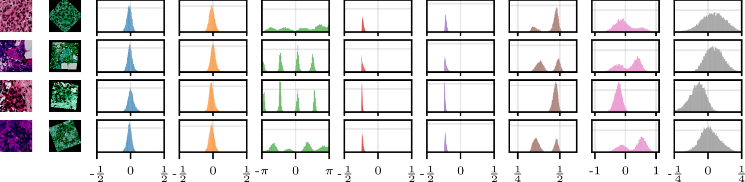
In this section, we provide a “negative” result for our SGM when applied to the PatchCamelyon dataset [Veeling et al., 2018]. The examples in this dataset, unlike those used in Section˜4, contain “content” up to the boundaries of the images.
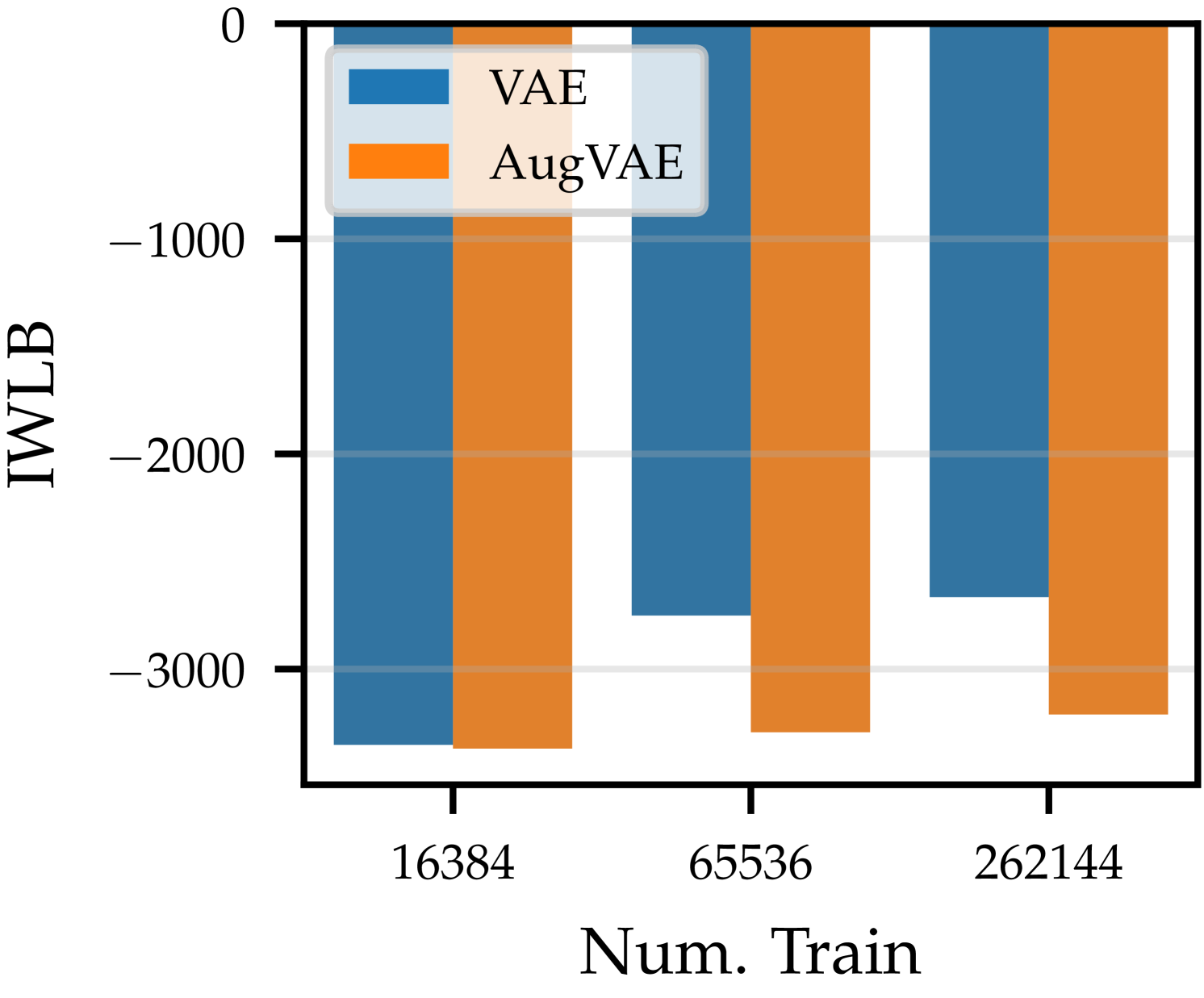
Figure˜16 shows examples of the prototypes and learned distributions for this dataset, with affine and color transformations. We allowed the model to learn any rotations within , while the actual dataset has a rotational invariance of . We see that in some cases the prototypes are rotated by close to relative to the original images. In other cases, the rotation of the prototypes relative to the original images is closer to . In the latter case, the learned distribution over rotation is close to the true distribution, but in the former case, the model learns a distribution that is closer to uniform. As a result, the resampled digits often display boundary effects that are not present in the original dataset. Otherwise, our SGM has learned reasonable distributions for translation, scaling, and HSV transformations.
Figure˜17 compares a standard VAE with AugVAE, an SGM-VAE hybrid model. We see that for small amounts of data, the VAE and AugVAE perform similarly. However, as the amount of training data increases, the VAE performs better. This is likely because the SGM has not learned the true distribution over rotations.
This “negative” result highlights the importance of correctly choosing the prior transformation distributions in certain settings. In this case, the performance of the SGM would have been improved by choosing a categorical distribution over rotations.
E.3 Additional Experiments
In this section, we provide additional plots to supplement those in Section˜4.
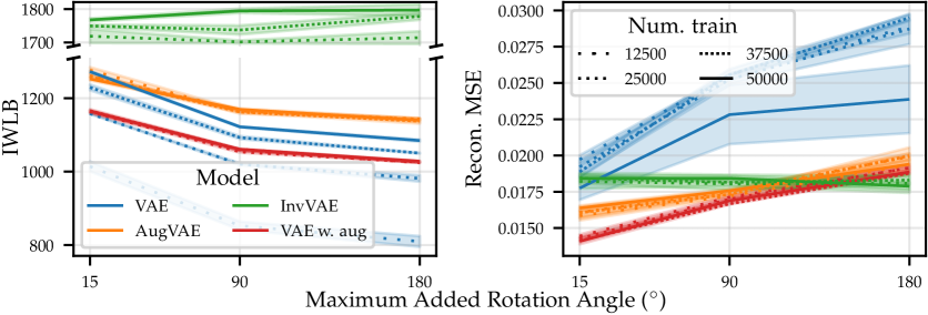
Figure˜18 extends the results in Figure˜11 to by including an additional metric: reconstruction MSE. Our findings with IWLB are consistent for this metric.
Figure˜19 expands on Figure˜8(b) in two ways. Firstly, it makes it clear that our inference network is able to provide the same or very similar prototype for observations in the same orbit. Secondly, it provides many more resampled examples of each digit, further demonstrating that our SGM has correctly captured the symmetries present in the dataset. Figure˜20 expands on Figure˜8(c) in the same way.
Figure˜21 extends Figure˜9 by including all of the digits shown in Figure˜19. The conclusions are much the same as before. We see that the learned distributions all make sense, especially for the most easily interpretable transformation parameter, rotation angle. Again, we note that smaller and bigger prototypes have appropriately different scaling distributions. Figure˜22 provides the learnt marginal distributions for the digits in Figure˜20. Here, we manually controlled the distributions over hue and saturation when loading the dataset, so we know that the range of the hue distribution should be approximately , while the range of the saturation distribution should be around . We see that this is indeed the case. We did not control the value of the images, so it is more difficult to interpret those. However, given that most (non-black) pixels are bright (i.e., close to 1) it makes sense that our SGM learns multiplicative values closer to 1.
Finally, Figure˜23 extends our dSprites results in two ways. Firstly, it provides many more resampled sprites, which also serves to demonstrate further that our SGM has captured the symmetries correctly. Secondly, the figure includes empirical distributions of positions of each of the classes of digits, which we have carefully controlled as described in Section˜C.3.1. These empirical distributions for the dataset are compared with empirical distributions for our resampled sprites. We see that although the resampled densities don’t match the original densities perfectly, their general shapes and ranges are correct.
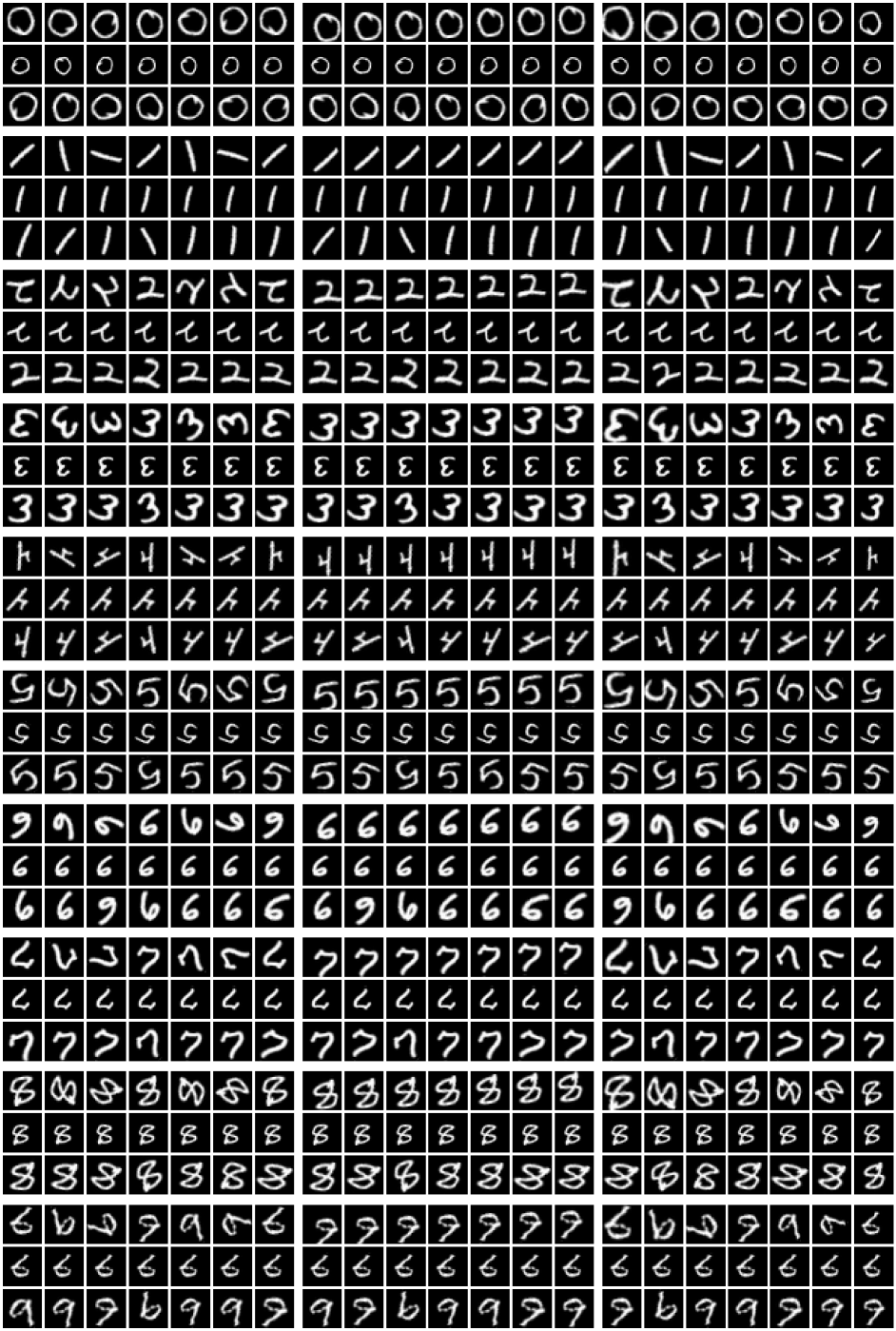
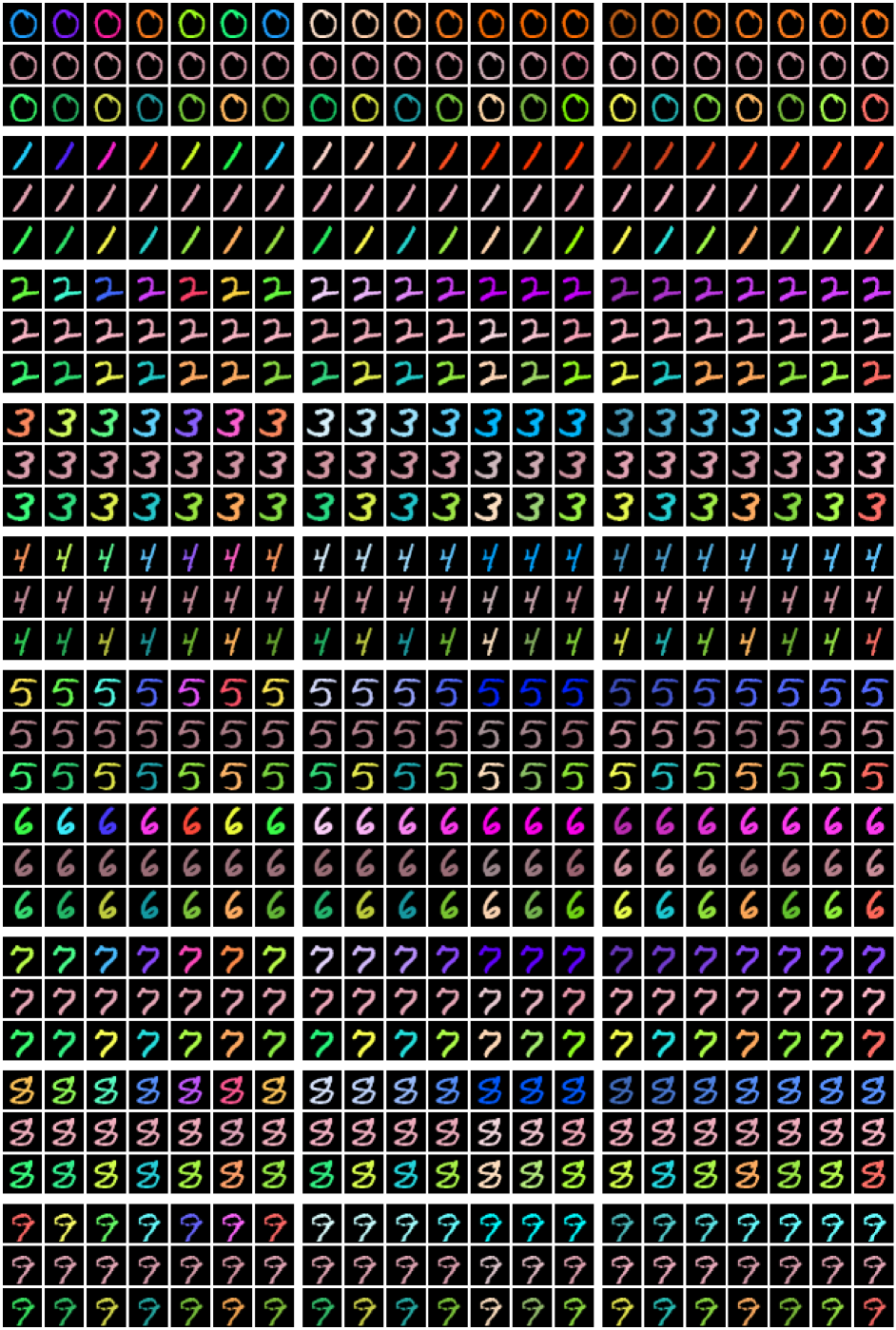
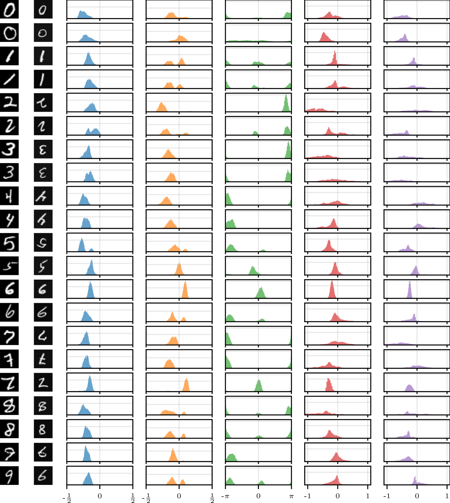
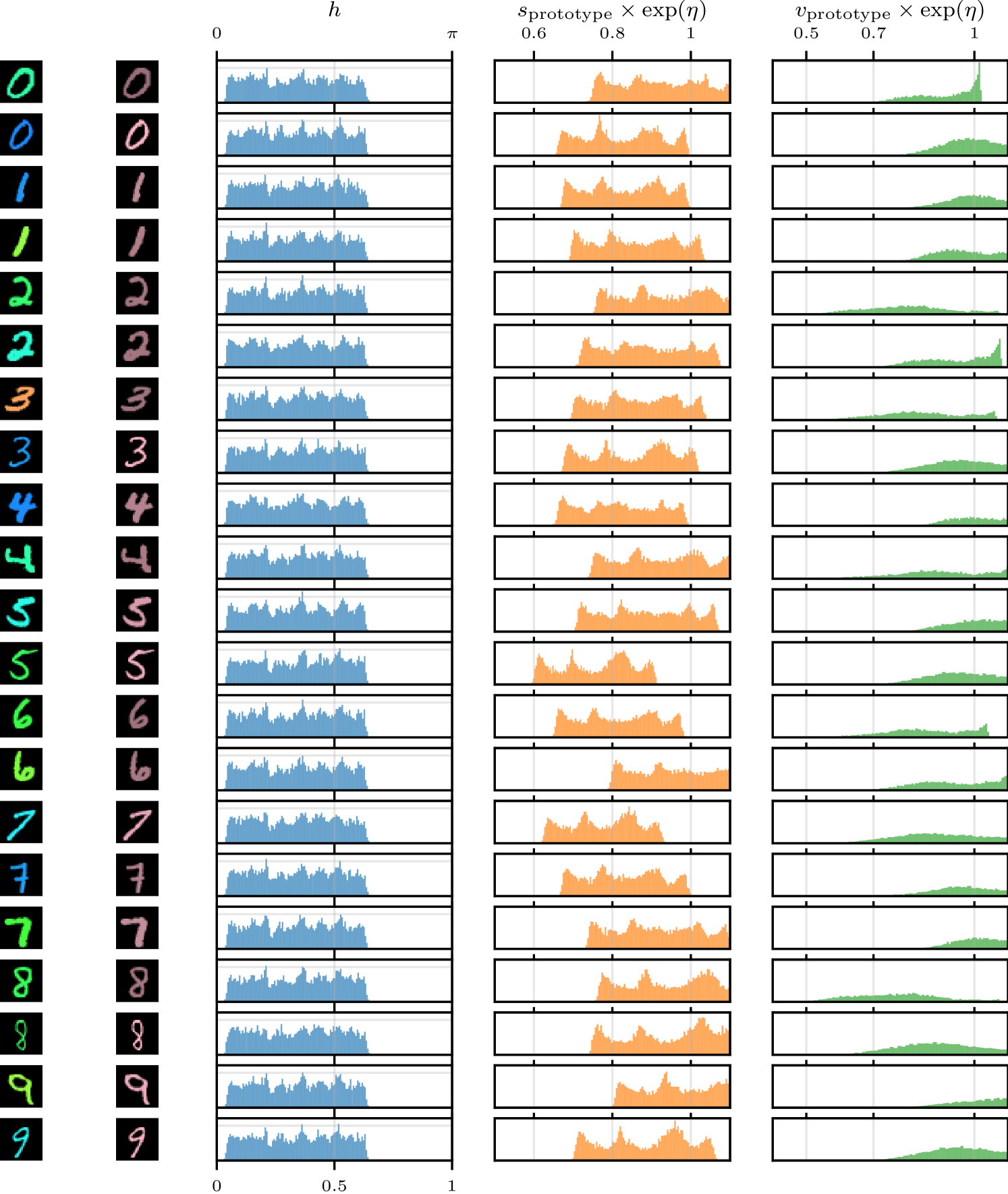
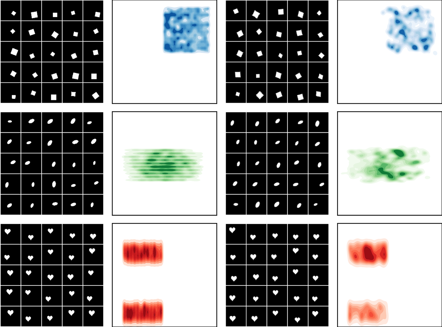
NeurIPS Paper Checklist
-
1.
Claims
-
Question: Do the main claims made in the abstract and introduction accurately reflect the paper’s contributions and scope?
-
Answer: [Yes]
-
Justification: In this paper we present a novel generative model of symmetry transformations. In our abstract and conclusion make two claims about this model: (1) it can accurately capture the symmetries in a dataset, and (2) when combined with a standard generative model we see improvements in data-efficiency. We believe that both of these claims reflect the paper’s contributions well. In the introduction, we also discuss some aspirational goals for disentanglement and scientific discovery, however, we are clear that these are not the focus of the paper.
-
Guidelines:
-
•
The answer NA means that the abstract and introduction do not include the claims made in the paper.
-
•
The abstract and/or introduction should clearly state the claims made, including the contributions made in the paper and important assumptions and limitations. A No or NA answer to this question will not be perceived well by the reviewers.
-
•
The claims made should match theoretical and experimental results, and reflect how much the results can be expected to generalize to other settings.
-
•
It is fine to include aspirational goals as motivation as long as it is clear that these goals are not attained by the paper.
-
•
-
2.
Limitations
-
Question: Does the paper discuss the limitations of the work performed by the authors?
-
Answer: [Yes]
-
Justification: Throughout the paper we provide footnotes to clarify the scope of our claims and point out their limitations (e.g., footnote 1 clarifies that our generative model does not always match the true generative process of the data). We also provide a detailed list of potential issues when using our method in practice. Furthermore, in our conclusion, we note that our method only learns approximate symmetries and requires a super-set of possible symmetries in the data to be specified. Finally, we provide some “negative results” in Section˜E.2, which are also mentioned as a limitation in our conclusion.
-
Guidelines:
-
•
The answer NA means that the paper has no limitation while the answer No means that the paper has limitations, but those are not discussed in the paper.
-
•
The authors are encouraged to create a separate "Limitations" section in their paper.
-
•
The paper should point out any strong assumptions and how robust the results are to violations of these assumptions (e.g., independence assumptions, noiseless settings, model well-specification, asymptotic approximations only holding locally). The authors should reflect on how these assumptions might be violated in practice and what the implications would be.
-
•
The authors should reflect on the scope of the claims made, e.g., if the approach was only tested on a few datasets or with a few runs. In general, empirical results often depend on implicit assumptions, which should be articulated.
-
•
The authors should reflect on the factors that influence the performance of the approach. For example, a facial recognition algorithm may perform poorly when image resolution is low or images are taken in low lighting. Or a speech-to-text system might not be used reliably to provide closed captions for online lectures because it fails to handle technical jargon.
-
•
The authors should discuss the computational efficiency of the proposed algorithms and how they scale with dataset size.
-
•
If applicable, the authors should discuss possible limitations of their approach to address problems of privacy and fairness.
-
•
While the authors might fear that complete honesty about limitations might be used by reviewers as grounds for rejection, a worse outcome might be that reviewers discover limitations that aren’t acknowledged in the paper. The authors should use their best judgment and recognize that individual actions in favor of transparency play an important role in developing norms that preserve the integrity of the community. Reviewers will be specifically instructed to not penalize honesty concerning limitations.
-
•
-
3.
Theory Assumptions and Proofs
-
Question: For each theoretical result, does the paper provide the full set of assumptions and a complete (and correct) proof?
-
Answer: [N/A]
-
Justification: This paper contains no theoretical results.
-
Guidelines:
-
•
The answer NA means that the paper does not include theoretical results.
-
•
All the theorems, formulas, and proofs in the paper should be numbered and cross-referenced.
-
•
All assumptions should be clearly stated or referenced in the statement of any theorems.
-
•
The proofs can either appear in the main paper or the supplemental material, but if they appear in the supplemental material, the authors are encouraged to provide a short proof sketch to provide intuition.
-
•
Inversely, any informal proof provided in the core of the paper should be complemented by formal proofs provided in appendix or supplemental material.
-
•
Theorems and Lemmas that the proof relies upon should be properly referenced.
-
•
-
4.
Experimental Result Reproducibility
-
Question: Does the paper fully disclose all the information needed to reproduce the main experimental results of the paper to the extent that it affects the main claims and/or conclusions of the paper (regardless of whether the code and data are provided or not)?
-
Answer: [Yes]
-
Justification: We provide a clear algorithm description (Algorithm˜1), discussions of all of the practical issues encountered when implementing our method (Sections˜3.1 and B, and detailed experimental setup descriptions—including dataset splits, model architectures, hyper-parameter settings and sweeps, transformation parameterisations, and a list of software libraries used—(Appendix˜C).
-
Guidelines:
-
•
The answer NA means that the paper does not include experiments.
-
•
If the paper includes experiments, a No answer to this question will not be perceived well by the reviewers: Making the paper reproducible is important, regardless of whether the code and data are provided or not.
-
•
If the contribution is a dataset and/or model, the authors should describe the steps taken to make their results reproducible or verifiable.
-
•
Depending on the contribution, reproducibility can be accomplished in various ways. For example, if the contribution is a novel architecture, describing the architecture fully might suffice, or if the contribution is a specific model and empirical evaluation, it may be necessary to either make it possible for others to replicate the model with the same dataset, or provide access to the model. In general. releasing code and data is often one good way to accomplish this, but reproducibility can also be provided via detailed instructions for how to replicate the results, access to a hosted model (e.g., in the case of a large language model), releasing of a model checkpoint, or other means that are appropriate to the research performed.
-
•
While NeurIPS does not require releasing code, the conference does require all submissions to provide some reasonable avenue for reproducibility, which may depend on the nature of the contribution. For example
-
(a)
If the contribution is primarily a new algorithm, the paper should make it clear how to reproduce that algorithm.
-
(b)
If the contribution is primarily a new model architecture, the paper should describe the architecture clearly and fully.
-
(c)
If the contribution is a new model (e.g., a large language model), then there should either be a way to access this model for reproducing the results or a way to reproduce the model (e.g., with an open-source dataset or instructions for how to construct the dataset).
-
(d)
We recognize that reproducibility may be tricky in some cases, in which case authors are welcome to describe the particular way they provide for reproducibility. In the case of closed-source models, it may be that access to the model is limited in some way (e.g., to registered users), but it should be possible for other researchers to have some path to reproducing or verifying the results.
-
(a)
-
•
-
5.
Open access to data and code
-
Question: Does the paper provide open access to the data and code, with sufficient instructions to faithfully reproduce the main experimental results, as described in supplemental material?
-
Answer: [Yes]
-
Justification: We have provided a link to a GitHub repository. We have provided instructions, model configurations, training scripts, and plotting notebooks to reproduce the main results from the paper.
-
Guidelines:
-
•
The answer NA means that paper does not include experiments requiring code.
-
•
Please see the NeurIPS code and data submission guidelines (https://nips.cc/public/guides/CodeSubmissionPolicy) for more details.
-
•
While we encourage the release of code and data, we understand that this might not be possible, so “No” is an acceptable answer. Papers cannot be rejected simply for not including code, unless this is central to the contribution (e.g., for a new open-source benchmark).
-
•
The instructions should contain the exact command and environment needed to run to reproduce the results. See the NeurIPS code and data submission guidelines (https://nips.cc/public/guides/CodeSubmissionPolicy) for more details.
-
•
The authors should provide instructions on data access and preparation, including how to access the raw data, preprocessed data, intermediate data, and generated data, etc.
-
•
The authors should provide scripts to reproduce all experimental results for the new proposed method and baselines. If only a subset of experiments are reproducible, they should state which ones are omitted from the script and why.
-
•
At submission time, to preserve anonymity, the authors should release anonymized versions (if applicable).
-
•
Providing as much information as possible in supplemental material (appended to the paper) is recommended, but including URLs to data and code is permitted.
-
•
-
6.
Experimental Setting/Details
-
Question: Does the paper specify all the training and test details (e.g., data splits, hyperparameters, how they were chosen, type of optimizer, etc.) necessary to understand the results?
-
Answer: [Yes]
-
Justification: We provide detailed experimental setup descriptions—including dataset splits, model architectures, hyper-parameter settings and sweeps, transformation parameterisations, and a list of software libraries used—in Appendix˜C.
-
Guidelines:
-
•
The answer NA means that the paper does not include experiments.
-
•
The experimental setting should be presented in the core of the paper to a level of detail that is necessary to appreciate the results and make sense of them.
-
•
The full details can be provided either with the code, in appendix, or as supplemental material.
-
•
-
7.
Experiment Statistical Significance
-
Question: Does the paper report error bars suitably and correctly defined or other appropriate information about the statistical significance of the experiments?
-
Answer: [Yes]
-
Justification: For all quantitative results, we report the mean and standard error over 3 random seeds.
-
Guidelines:
-
•
The answer NA means that the paper does not include experiments.
-
•
The authors should answer "Yes" if the results are accompanied by error bars, confidence intervals, or statistical significance tests, at least for the experiments that support the main claims of the paper.
-
•
The factors of variability that the error bars are capturing should be clearly stated (for example, train/test split, initialization, random drawing of some parameter, or overall run with given experimental conditions).
-
•
The method for calculating the error bars should be explained (closed form formula, call to a library function, bootstrap, etc.)
-
•
The assumptions made should be given (e.g., Normally distributed errors).
-
•
It should be clear whether the error bar is the standard deviation or the standard error of the mean.
-
•
It is OK to report 1-sigma error bars, but one should state it. The authors should preferably report a 2-sigma error bar than state that they have a 96% CI, if the hypothesis of Normality of errors is not verified.
-
•
For asymmetric distributions, the authors should be careful not to show in tables or figures symmetric error bars that would yield results that are out of range (e.g. negative error rates).
-
•
If error bars are reported in tables or plots, The authors should explain in the text how they were calculated and reference the corresponding figures or tables in the text.
-
•
-
8.
Experiments Compute Resources
-
Question: For each experiment, does the paper provide sufficient information on the computer resources (type of compute workers, memory, time of execution) needed to reproduce the experiments?
-
Answer: [Yes]
-
Justification: See Appendix˜D for estimates of the compute costs, in the form of A100 GPU days, for the whole project as well as each of the figures in the main text.
-
Guidelines:
-
•
The answer NA means that the paper does not include experiments.
-
•
The paper should indicate the type of compute workers CPU or GPU, internal cluster, or cloud provider, including relevant memory and storage.
-
•
The paper should provide the amount of compute required for each of the individual experimental runs as well as estimate the total compute.
-
•
The paper should disclose whether the full research project required more compute than the experiments reported in the paper (e.g., preliminary or failed experiments that didn’t make it into the paper).
-
•
-
9.
Code Of Ethics
-
Question: Does the research conducted in the paper conform, in every respect, with the NeurIPS Code of Ethics https://neurips.cc/public/EthicsGuidelines?
-
Answer: [Yes]
-
Justification: We have read and acknowledged the NeurIPS Code of Ethics. We believe that our paper conforms with this code in every respect.
-
Guidelines:
-
•
The answer NA means that the authors have not reviewed the NeurIPS Code of Ethics.
-
•
If the authors answer No, they should explain the special circumstances that require a deviation from the Code of Ethics.
-
•
The authors should make sure to preserve anonymity (e.g., if there is a special consideration due to laws or regulations in their jurisdiction).
-
•
-
10.
Broader Impacts
-
Question: Does the paper discuss both potential positive societal impacts and negative societal impacts of the work performed?
-
Answer: [N/A]
-
Justification: Our work is foundational research that is not tied to any particular application for which we see a direct path to negative applications.
-
Guidelines:
-
•
The answer NA means that there is no societal impact of the work performed.
-
•
If the authors answer NA or No, they should explain why their work has no societal impact or why the paper does not address societal impact.
-
•
Examples of negative societal impacts include potential malicious or unintended uses (e.g., disinformation, generating fake profiles, surveillance), fairness considerations (e.g., deployment of technologies that could make decisions that unfairly impact specific groups), privacy considerations, and security considerations.
-
•
The conference expects that many papers will be foundational research and not tied to particular applications, let alone deployments. However, if there is a direct path to any negative applications, the authors should point it out. For example, it is legitimate to point out that an improvement in the quality of generative models could be used to generate deepfakes for disinformation. On the other hand, it is not needed to point out that a generic algorithm for optimizing neural networks could enable people to train models that generate Deepfakes faster.
-
•
The authors should consider possible harms that could arise when the technology is being used as intended and functioning correctly, harms that could arise when the technology is being used as intended but gives incorrect results, and harms following from (intentional or unintentional) misuse of the technology.
-
•
If there are negative societal impacts, the authors could also discuss possible mitigation strategies (e.g., gated release of models, providing defenses in addition to attacks, mechanisms for monitoring misuse, mechanisms to monitor how a system learns from feedback over time, improving the efficiency and accessibility of ML).
-
•
-
11.
Safeguards
-
Question: Does the paper describe safeguards that have been put in place for responsible release of data or models that have a high risk for misuse (e.g., pretrained language models, image generators, or scraped datasets)?
-
Answer: [N/A]
-
Justification: Our work does not pose such risks.
-
Guidelines:
-
•
The answer NA means that the paper poses no such risks.
-
•
Released models that have a high risk for misuse or dual-use should be released with necessary safeguards to allow for controlled use of the model, for example by requiring that users adhere to usage guidelines or restrictions to access the model or implementing safety filters.
-
•
Datasets that have been scraped from the Internet could pose safety risks. The authors should describe how they avoided releasing unsafe images.
-
•
We recognize that providing effective safeguards is challenging, and many papers do not require this, but we encourage authors to take this into account and make a best faith effort.
-
•
-
12.
Licenses for existing assets
-
Question: Are the creators or original owners of assets (e.g., code, data, models), used in the paper, properly credited and are the license and terms of use explicitly mentioned and properly respected?
-
Answer: [Yes]
-
Justification: We cite and provide licenses for all of the datasets used in this paper.
-
Guidelines:
-
•
The answer NA means that the paper does not use existing assets.
-
•
The authors should cite the original paper that produced the code package or dataset.
-
•
The authors should state which version of the asset is used and, if possible, include a URL.
-
•
The name of the license (e.g., CC-BY 4.0) should be included for each asset.
-
•
For scraped data from a particular source (e.g., website), the copyright and terms of service of that source should be provided.
-
•
If assets are released, the license, copyright information, and terms of use in the package should be provided. For popular datasets, paperswithcode.com/datasets has curated licenses for some datasets. Their licensing guide can help determine the license of a dataset.
-
•
For existing datasets that are re-packaged, both the original license and the license of the derived asset (if it has changed) should be provided.
-
•
If this information is not available online, the authors are encouraged to reach out to the asset’s creators.
-
•
-
13.
New Assets
-
Question: Are new assets introduced in the paper well documented and is the documentation provided alongside the assets?
-
Answer: [N/A]
-
Justification: Our paper does not release any new assets.
-
Guidelines:
-
•
The answer NA means that the paper does not release new assets.
-
•
Researchers should communicate the details of the dataset/code/model as part of their submissions via structured templates. This includes details about training, license, limitations, etc.
-
•
The paper should discuss whether and how consent was obtained from people whose asset is used.
-
•
At submission time, remember to anonymize your assets (if applicable). You can either create an anonymized URL or include an anonymized zip file.
-
•
-
14.
Crowdsourcing and Research with Human Subjects
-
Question: For crowdsourcing experiments and research with human subjects, does the paper include the full text of instructions given to participants and screenshots, if applicable, as well as details about compensation (if any)?
-
Answer: [N/A]
-
Justification: We did not make use of any crowdsourcing or human subjects.
-
Guidelines:
-
•
The answer NA means that the paper does not involve crowdsourcing nor research with human subjects.
-
•
Including this information in the supplemental material is fine, but if the main contribution of the paper involves human subjects, then as much detail as possible should be included in the main paper.
-
•
According to the NeurIPS Code of Ethics, workers involved in data collection, curation, or other labor should be paid at least the minimum wage in the country of the data collector.
-
•
-
15.
Institutional Review Board (IRB) Approvals or Equivalent for Research with Human Subjects
-
Question: Does the paper describe potential risks incurred by study participants, whether such risks were disclosed to the subjects, and whether Institutional Review Board (IRB) approvals (or an equivalent approval/review based on the requirements of your country or institution) were obtained?
-
Answer: [N/A]
-
Justification: We did not make use of any crowdsourcing or human subjects.
-
Guidelines:
-
•
The answer NA means that the paper does not involve crowdsourcing nor research with human subjects.
-
•
Depending on the country in which research is conducted, IRB approval (or equivalent) may be required for any human subjects research. If you obtained IRB approval, you should clearly state this in the paper.
-
•
We recognize that the procedures for this may vary significantly between institutions and locations, and we expect authors to adhere to the NeurIPS Code of Ethics and the guidelines for their institution.
-
•
For initial submissions, do not include any information that would break anonymity (if applicable), such as the institution conducting the review.
-
•