A generic coordinate descent solver for nonsmooth convex optimization
Abstract
We present a generic coordinate descent solver for the minimization of a nonsmooth convex objective with structure. The method can deal in particular with problems with linear constraints. The implementation makes use of efficient residual updates and automatically determines which dual variables should be duplicated. A list of basic functional atoms is pre-compiled for efficiency and a modelling language in Python allows the user to combine them at run time. So, the algorithm can be used to solve a large variety of problems including Lasso, sparse multinomial logistic regression, linear and quadratic programs.
keywords:
Coordinate descent; convex optimization; generic solver; efficient implementation1 Introduction
Coordinate descent methods decompose a large optimization problem into a sequence of one-dimensional optimization problems. The algorithm was first described for the minimization of quadratic functions by Gauss and Seidel in [49]. Coordinate descent methods have become unavoidable in machine learning because they are very efficient for key problems, namely Lasso [20], logistic regression [67] and support vector machines [43, 52]. Moreover, the decomposition into small subproblems means that only a small part of the data is processed at each iteration and this makes coordinate descent easily scalable to high dimensions.
One of the main ingredients of an efficient coordinate descent solver is its ability to compute efficiently partial derivatives of the objective function [39]. In the case of least squares for instance, this involves the definition of a vector of residuals that will be updated during the run of the algorithm. As this operation needs to be performed at each iteration, and millions of iterations are usually needed, the residual update and directional derivative computation must be coded in a compiled programming language.
Many coordinate descent solvers have been written in order to solve a large variety of problems. However, most of the existing solvers can only solve problems of the type
where is the th block of , , is a matrix and is a vector, and where is a convex differentiable function and is a convex lower-semicontinuous function whose proximal operator is easy to compute (a.k.a. a proximal-friendly convex function). Each piece of code usually covers only one type of function [14, 42]. Moreover, even when the user has a choice of objective function, the same function is used for every block [6].
In this work, we propose a generic coordinate descent method for the resolution of the convex optimization problem
| (1) |
We shall call , and atom functions. Each of them may be different. We will assume that ’s are differentiable and convex, ’s and ’s are proximal-friendly convex functions. As before and are matrices, is a multiple of the identity matrix of size , , and are vectors, , and are positive real numbers, is a positive semi-definite matrix.
The algorithm we implemented is described in [15] and can be downloaded on https://bitbucket.org/ofercoq/cd_solver. The present paper focuses on important implementation details about residual updates and dual variable duplication. The novelty of our code is that it allows a generic treatment of these algorithmic steps and includes a modelling interface in Python for the definition of the optimization problem. Note that unlike most coordinate descent implementations, it can deal with nonseparable nonsmooth objectives and linear constraints.
2 Literature review on coordinate descent methods
A thorough review on coordinate descent is beyond the scope of this paper. We shall refer the interested reader to the review papers [63] and [54]. Instead, for selected papers dealing with smooth functions, separable non-smooth functions or non-separable non-smooth function, we list their main features. We also quickly review what has been done for non-convex functions. We sort papers in order of publication except when there are an explicit dependency between a paper and a follow-up.
2.1 Smooth functions
Smooth objectives are a natural starting point for algorithmic innovations. The optimization problem at stake writes
where is a convex differentiable function with Lipschitz-continuous partial derivatives.
In Table 1, we compare papers that introduced important improvements to coordinate descent methods. We shall in particular stress the seminal paper by Tseng and Yun [60]. It features coordinate gradient steps instead of exact minimization. Indeed a coordinate gradient steps gives similar iteration complexity both in theory and in practice for a much cheaper iteration cost. Moreover, this opened the door for many innovations: blocks of coordinates and the use of proximal operators were developed in the same paper. Another crucial step was made in [39]: Nesterov showed how randomization can help finding finite-time complexity bounds and proposed an accelerated version of coordinate descent. He also proposed to use a non-uniform sampling of coordinates depending on the coordinate-wise Lipschitz constants.
| Paper | Rate | Rand | Grad | Blck | Par | Acc | Notable feature |
|---|---|---|---|---|---|---|---|
| Seidel ’74 [49] | N | quadratic | |||||
| Warga ’63 [62] | N | strictly convex | |||||
| Luo & Tseng ’92 [34] | asymp | N | rate for weakly convex | ||||
| Leventhal & Lewis ’08 [28] | ✓ | Y | quadratic | ||||
| Tseng & Yun ’09 [60] | asymp | N | ✓ | ✓ | line search, proximal operator | ||
| Nesterov ’12 [39] | ✓ | Y | ✓ | not eff | 1st acc & 1st non-uniform | ||
| Beck & Tetruashvili ’13 [4] | ✓ | N | ✓ | ✓ | not eff | finite time analysis cyclic CD | |
| Lin & Xiao ’13 [33] | ✓ | Y | ✓ | ✓ | not eff | improvements on [39, 47] | |
| Lee & Sidford ’13 [27] | ✓ | Y | ✓ | ✓ | 1st efficient accelerated | ||
| Liu et al ’13 [31] | ✓ | Y | ✓ | ✓ | 1st asynchronous | ||
| Glasmachers & Dogan ’13 [22] | Y | ✓ | heuristic sampling | ||||
| Richtárik & Takáč ’16 [46] | ✓ | Y | ✓ | ✓ | 1st arbitrary sampling | ||
| Allen-Zhu et al ’16 [2] | ✓ | Y | ✓ | ✓ | ✓ | non-uniform sampling | |
| Sun et al ’17 [55] | ✓ | Y | ✓ | ✓ | ✓ | better asynchrony than [31] |
2.2 Separable non-smooth functions
A large literature has been devoted to composite optimization problems with separable non-smooth functions:
where is a convex differentiable function with Lipschitz-continuous partial derivatives and for all , is a convex function whose proximal operator is easy to compute. Indeed, regularized expected risk minimization problems often fit into this framework and this made the success of coordinate descent methods for machine learning applications.
Some papers study , where is strongly convex and apply coordinate descent to a dual problem written as
One of the challenges of these works is to show that even though we are solving the dual problem, one can still recover rates for a sequence minimizing the primal objective.
We present our selection of papers devoted to this type of problems in Table 2.
| Paper | Prx | Par | Acc | Dual | Notable feature |
|---|---|---|---|---|---|
| Tseng & Yun ’09 [60] | ✓ | 1st prox, line search, deterministic | |||
| S-Shwartz & Tewari ’09 [50] | 1st -regularized w finite time bound | ||||
| Bradley et al ’11 [7] | ✓ | -regularized parallel | |||
| Richtárik & Takáč ’14 [47] | ✓ | 1st proximal with finite time bound | |||
| S-Shwartz & Zhang ’13 [51] | ✓ | ✓ | 1st dual | ||
| Richtárik & Takáč ’15 [48] | ✓ | ✓ | 1st general parallel | ||
| Takáč et al ’13 [56] | ✓ | ✓ | ✓ | 1st dual & parallel | |
| S-Shwartz & Zhang ’14 [53] | ✓ | ✓ | ✓ | acceleration in the primal | |
| Yun ’14 [68] | ✓ | analysis of cyclic CD | |||
| Fercoq & Richtárik ’15 [18] | ✓ | ✓ | ✓ | 1st proximal and accelerated | |
| Lin, Lu & Xiao ’14 [30] | ✓ | ✓ | prox & accelerated on strong conv. | ||
| Richtárik & Takáč ’16 [45] | ✓ | ✓ | 1st distributed | ||
| Fercoq et al ’14 [17] | ✓ | ✓ | ✓ | distributed computation | |
| Lu & Xiao ’15 [33] | ✓ | improved complexity over [47, 39] | |||
| Li & Lin ’18 [29] | ✓ | ✓ | ✓ | acceleration in the dual | |
| Fercoq & Qu ’18 [16] | ✓ | ✓ | restart for obj with error bound |
2.3 Non-separable non-smooth functions
Non-separable non-smooth objective functions are much more challenging to coordinate descent methods. One wishes to solve
where is a convex differentiable function with Lipschitz-continuous partial derivatives, and are convex functions whose proximal operator are easy to compute and is a linear operator. Indeed, the linear operator introduces a coupling between the coordinates and a naive approach leads to a method that does not converge to a minimizer [3]. When , the convex indicator function of the set , we have equality constraints.
We present our selection of papers devoted to this type of problems in Table 3.
| Paper | Rate | Const | PD-CD | Notable feature |
| Platt ’99 [43] | ✓ | P | for SVM | |
| Tseng & Yun ’09 [61] | ✓ | ✓ | P | adapts Gauss-Southwell rule |
| Tao et al ’12 [57] | ✓ | P | uses averages of subgradients | |
| Necoara et al ’12 [38] | ✓ | ✓ | P | 2-coordinate descent |
| Nesterov ’12 [40] | ✓ | P | uses subgradients | |
| Necoara & Clipici ’13 [37] | ✓ | ✓ | P | coupled constraints |
| Combettes & Pesquet ’14 [11] | ✓ | ✓ | 1st PD-CD, short step sizes | |
| Bianchi et al ’14 [5] | ✓ | ✓ | distributed optimization | |
| Hong et al ’14 [24] | ✓ | updates all dual variables | ||
| Fercoq & Richtárik ’17 [19] | ✓ | P | uses smoothing | |
| Alacaoglu et al ’17 [1] | ✓ | ✓ | ✓ | 1st PD-CD w rate for constraints |
| Xu & Zhang ’18 [66] | ✓ | ✓ | better rate than [21] | |
| Chambolle et al ’18 [9] | ✓ | ✓ | updates all primal variables | |
| Fercoq & Bianchi ’19 [15] | ✓ | ✓ | ✓ | 1st PD-CD w long step sizes |
| Gao et al ’19 [21] | ✓ | ✓ | 1st primal-dual w rate for constraints | |
| Latafat et al ’19 [26] | ✓ | ✓ | ✓ | linear conv w growth condition |
2.4 Non-convex functions
The goal here is to find a local minimum to the problem
without any assumption on the convexity of nor . The function should be continuously differentiable and the proximal operator of each function should be easily computable. Note that in the non-convex setting, the proximal operator may be set-valued.
| Paper | Conv | Smth | Nsmth | Notable feature |
|---|---|---|---|---|
| Grippo & Sciandrone ’00 [23] | ✓ | 2-block or coordinate-wise quasiconvex | ||
| Tseng & Yun ’09 [60] | ✓ | ✓ | convergence under error bound | |
| Hsieh & Dhillon ’11 [25] | ✓ | non-negative matrix factorization | ||
| Breheny & Huang ’11 [8] | ✓ | regularized least squares | ||
| Mazumder et al ’11 [35] | ✓ | regularized least squares | ||
| Razaviyayn et al ’13 [44] | ✓ | ✓ | requires uniqueness of the prox | |
| Xu & Yin ’13 [64] | ✓ | ✓ | multiconvex | |
| Lu & Xiao ’13 [32] | ✓ | ✓ | random sampling | |
| Patrascu & Necoara ’15 [41] | ✓ | ✓ | randomized + 1 linear constraint | |
| Xu & Yin ’17 [65] | ✓ | ✓ | ✓ | convergence under KL |
3 Description of the Algorithm
3.1 General scheme
The algorithm we implemented is a coordinate descent primal-dual method developed in [15]. Let introduce the notation , , , , , and the spectral radius of matrix . We shall also denote , , the matrix which stacks the matrices and the matrix which stacks the matrices . The algorithm writes then as Algorithm 1.
Input: Differentiable function , matrix , functions and whose proximal operators are available.
Initialization: Choose , . Denote , , and the spectral radius of matrix . Choose step sizes and such that ,
| (2) |
For all , set .
For all , set
.
Iteration : Define:
For and for each , update:
Otherwise, set , , and .
We will denote the columns of the identity matrix corresponding to the blocks of , so that and the columns of the identity matrix corresponding to the blocks of .
3.2 Computation of partial derivatives
For simplicity of implementation, we are assuming that is separable and the blocks of variable will follow the block structure of . This implies in particular that at each iteration, only needs to be computed. This partial derivative needs to be calculated efficiently because it needs to be performed at each iteration of the algorithm. We now describe the efficient residual update method, which is classically used in coordinate descent implementations [39].
Denote and . By the chain rule, we have
If and are pre-computed, only operations are needed.
For an efficient implementation, we will update the residuals as follows, using the fact that only the coordinate block is updated:
Hence, updating also requires only iterations.
Similarly, updating the residuals , , and can be done in and operations.
Although this technique is well known, it is not trivial how to write it in a generic fashion, since residual updates are needed at each iteration and should be written in a compiled language. We coded the residual update using abstract atom functions in order to achieve this goal.
3.3 Computation of proximal operators using atom functions
Another major step in the method is the computation of the coordinate of for a given .
As is assumed to be diagonal, is separable. Hence, by the change of variable ,
where we used the abuse of notation that is either the scaled identity matrix or any of its diagonal elements. This derivation shows that to compute we only need linear algebra and the proximal operator of the atom function .
We can similarly compute . To compute , we use Moreau’s formula:
3.4 Duplication of dual variables
Algorithm 1 maintains duplicated dual variables as well as averaged dual variables where and is of size . The sets for all are given by the sparse column format representation of . Yet, for all , we need to construct the set of indices of that need to be updated. This is the table dual_vars_to_update in the code. Moreover, as is not separable in general, in order to compute , for , we need to determine the set of dual indices that belong to the same block as with respect to the block decomposition of . This is the purpose of the tables inv_blocks_h and blocks_h.
The procedure allows us to only compute the entries of that are required for the update of .
4 Code structure
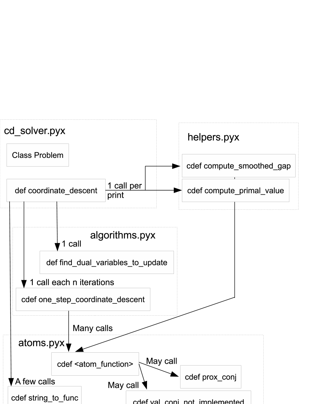
The code is organized in nine files. The main file is cd_solver.pyx. It contains the Python callable and the data structure for the problem definition. The other files are atoms.pyx/pxd, algorithm.pyx/pxd, helpers.pyx/pxd and screening.pyx/pxd. They contain the definition of the atom functions, the algorithms and the functions for computing the objective value. In Figure 1, we show for each subfunction, in which function it is used. The user needs to call the Python class Problem and the Python function coordinate_descent. Atom functions can be added by the user without modifying the main algorithm.
All tables are defined using Numpy’s array constructor in the coordinate_descent function. The main loop of coordinate descent and the atom functions are pre-compiled for efficiency.
5 Atom functions
The code allows us to define atom functions independently of the coordinate descent algorithm. As an example, we provide in Figure 2 the code for the square function atom.
cdef DOUBLE square(DOUBLE[:] x, DOUBLE[:] buff, int nb_coord, MODE mode,
        DOUBLE prox_param, DOUBLE prox_param2) nogil:
    # Function x -> x**2
    cdef int i
    cdef DOUBLE val = 0.
    if mode == GRAD:
        for i in range(nb_coord):
            buff[i] = 2. * x[i]
        return buff[0]
    elif mode == PROX:
        for i in range(nb_coord):
            buff[i] = x[i] / (1. + 2. * prox_param)
        return buff[0]
    elif mode == PROX_CONJ:
        return prox_conj(square, x, buff, nb_coord, prox_param, prox_param2)
    elif mode == LIPSCHITZ:
        buff[0] = 2.
        return buff[0]
    elif mode == VAL_CONJ:
        return val_conj_not_implemented(square, x, buff, nb_coord)
    else:  # mode == VAL
        for i in range(nb_coord):
            val += x[i] * x[i]
        return val
As inputs, it gets x (an array of numbers which is the point where the operation takes place), buff (the buffer for vectorial outputs), nb_coord (is the size of x), mode, prox_param and prox_param2 (numbers which are needed when computing the proximal operator). The input mode can be:
-
•
GRAD in order to compute the gradient.
-
•
PROX to compute the proximal operator.
-
•
PROX_CONJ uses Moreau’s formula to compute the proximal operator of the conjugate function.
-
•
LIPSCHITZ to return the Lipschitz constant of the gradient.
-
•
VAL_CONJ to return the value of the conjugate function. As this mode is used only by compute_smoothed_gap for printing purposes, its implementation is optional and can be approximated using the helper function val_conj_not_implemented. Indeed, for a small , , where .
-
•
VAL to return the value of the function.
Some functions naturally require multi-dimensional inputs, like or the log-sum-exp function. For consistency, we define all the atoms with multi-dimensional inputs: for an atom function , we extend it to an atom function by .
For efficiency purposes, we are bypassing the square atom function when computing a gradient and implemented it directly in the algorithm.
6 Modelling language
In order to use the code in all its generality, we defined a modelling language that can be used to define the optimization problem we want to solve (1).
The user defines a problem using the class Problem. Its arguments can be:
-
•
N the number of variables, blocks the blocks of coordinates coded in the same fashion as the indptr index of sparse matrices (default [0, 1, …, N]), x_init the initial primal point (default 0) and y_init the initial duplicated dual variable (default 0)
-
•
Lists of strings f, g and h that code for the atom functions used. The function string_to_func is responsible for linking the atom function that corresponds to the string. Our convention is that the string code is exactly the name of the function in atoms.pyx. The size of the input of each atom function is defined in blocks_f, blocks and blocks_h. The function strings f, g or h may be absent, which means that the function does not appear in the problem to solve.
-
•
Arrays and matrices cf, Af, bf, cg, Dg, bg, ch, Ah, bh, Q. The class initiator transforms matrices into the sparse column format and checks whether Dg is diagonal.
For instance, in order to solve the Lasso problem, , one can type
pb_lasso = cd_solver.Problem(N=A.shape[1], f=["square"]*A.shape[0], Af=A,
bf=b, cf=[0.5]*A.shape[0], g=["abs"]*A.shape[1], cg=[lambda]*A.shape[1])
cd_solver.coordinate_descent(pb_lasso)
7 Extensions
7.1 Non-uniform probabilities
We added the following feature for an improved efficiency. Under the argument sampling=’kink_half’, the algorithms periodically detects the set of blocks such that if is at a kink of . Then, block is selected with probability law
The rationale for this probability law is that blocks at kinks are likely to incur no move when we try to update them. We thus put more computational power for non-kinks. On the other hand, we still keep an update probability weight of at least for each block, so even in unfavourable cases, we should not observe too much degradation in the performance as compared to the uniform law.
7.2 Acceleration
We also coded accelerated coordinate descent [18], as well as its restarted [16] and primal-dual [1] variants. The algorithm is given in Algorithm 2. As before, and should not be computed: only the relevant coordinates should be computed.
Input: Differentiable function , matrix , functions and whose proximal operators are available.
Initialization: Choose , . Choose and denote .
Set , , , and .
Iteration : Define:
For , update:
Otherwise, set .
Compute as the unique positive root of
Update , and for all .
If Restart() is true:
Set .
Set and .
Reset , , , , .
The accelerated algorithms improve the worst case guarantee as explained in Table 5:
However, accelerated algorithms do not take profit of regularity properties of the objective like strong convexity. Hence, they are not guaranteed to be faster, even though restart may help.
7.3 Variable screening
The code includes the Gap Safe screening method presented in [36]. Note that the method has been studied only for the case where . Given a non-differentiability point of the function where the subdifferential has a non-empty interior, a test is derived to check whether is the variable of an optimal solution. If this is the case, one can set and stop updating this variable. This may lead to a huge speed up in some cases. As the test relies on the computation of the duality gap, which has a nonnegligible cost, it is only performed from time to time.
In order to state Gap Safe screening in a general setting, we need the concept of polar of a support function. Let be a convex set. The support function of is defined by
The polar to is
In particular, if , then . Denote , so that , , a solution to the optimization problem (1) and suppose we have a set such that . Gap Safe screening states that
Denote and 111We reuse the notation and here for the purpose of this section.. We choose as a sphere centered at
and with radius
where
and
Note that as is a rescaled version of , we do not need to know in order to compute . It is proved in [36] that this set contains for any optimal solutions to the primal problem. In the case where is a norm and , these expressions simplify since the is nothing else than the dual norm associated to .
For the estimation of , we use the fact that the polar of a support function is sublinear and positively homogeneous. Indeed, we have
Here is a point where has a nonempty interior. Some care should be taken when is unbounded, so that we first check whether for all .
Here also, the novelty lies in the genericity of the implementation.
8 Numerical validation
8.1 Performance
In order to evaluate the performance of the implementation, we compare our implementation with a pure Python coordinate descent solver and code written for specific problems: Scikit learn’s Lasso solver and Liblinear’s SVM solver. We run the code on an Intel Xeon CPU at 3.07GHz.
| Lasso | |
|---|---|
| Pure Python | 308.76s |
| cd_solver | 0.43s |
| Scikit learn Lasso | 0.11s |
| SVM | |
|---|---|
| Pure Python | 126.24s |
| cd_solver | 0.31s |
| Liblinear SVM | 0.13s |
We can see on Table 6 that our code is hundreds of times faster than the pure Python code. This is due to the compiled nature of our code, that does not suffer from the huge number of iterations required by coordinate descent. On the other hand, our code is about 4 times slower than state-of-the-art coordinate descent implementations designed for a specific problem. We can see it in both examples we chose. This overhead is the price of genericity.
We believe that, except for critical applications like Lasso or SVM, a 4 times speed-up does not justify writing a new code from scratch, since a separate piece of code for each problem makes it difficult to maintain and to improve with future algorithmic advances.
8.2 Genericity
We tested our algorithm on the following problems:
-
•
Lasso problem
-
•
Binomial logistic regression
where for all .
-
•
Sparse binomial logistic regression
-
•
Dual SVM without intercept
where is the convex indicator function of the set and encodes the constraint .
-
•
Dual SVM with intercept
-
•
Linearly constrained quadratic program
-
•
Linear program
-
•
TV+-regularized regression
where is the discrete gradient operator and .
-
•
Sparse multinomial logistic regression
where for all .
This list demonstrates that the method is able to deal with differentiable functions, separable or nonseparable nondifferentiable functions, as well as use several types of atom function in a single problem.
8.3 Benchmarking
In Table 7, we compare the performance of Algorithm 1 with and without screening, Algorithm 2 with and without screening as well as 2 alternative solvers for 3 problems exhibiting various situations:
-
•
Lasso: the nonsmooth function in the Lasso problem is separable;
-
•
the TV-regularized regression problem has a nonsmooth, nonseparable regularizer whose matrix is sparse;
-
•
the dual SVM with intercept has a single linear nonseparable constraint.
For Algorithm 2, we set the restart with a variable sequence as in [16]. We did not tune the algorithmic parameters for each instance. We evaluate the precision of a primal-dual pair as follows. We define the smoothed gap [59] as
and we choose the positive parameters and as
It is shown in [59] that when , and are small then the objective value and feasibility gaps are small.
For the Lasso problems, we compare our implementations of the coordinate descent method with scikit-learn’s coordinate descent [42] and CVXPY’s augmented Lagrangian method [12] called OSQP. As in Table 6, we have a factor 4 between Alg. 1 without screening and scikit-learn. Acceleration and screening allows us to reduce this gap without sacrificing generality. OSQP is efficient on small problems but is not competitive on larger instances.
For the TV-regularized regression problems, we compare ourself with FISTA where the proximal operator of the total variation is computed inexactly and with LBFGS where the total variation is smoothed with a decreasing smoothing parameter. Those two methods have been implemented for [13]. They manage to solve the problem to an acceptable accuracy in a few hours. As the problem is rather large, we did not run OSQP on it. For our methods, as is nonzero, we cannot use variable screening with the current theory. Alg. 1 quickly reduces the objective value but fails to get a high precision in a reasonable amount of time. On the other hand, Alg. 2 is the quickest among the four solvers tested here.
The third problem we tried is dual support vector machine with intercept. A very famous solver is libsvm [10], which implements SMO [43], a 2-coordinate descent method that ensures the feasibility of the constraints at each iteration. The conclusions are similar to what we have seen above. The specialized solver remains a natural choice. OSQP can only solve small instances. Alg. 1 has trouble finding high accuracy solutions. Alg. 2 is competitive with respect to the specialized solver.
| Problem | Dataset | Alternative solver 1 | Alternative solver 2 | Algorithm 1 | Algorithm 2 |
|---|---|---|---|---|---|
| Lasso () | triazines (=186, =60) | Scikit-learn: 0.005s | OSQP: 0.033s | 0.107s; scr: 0.101s | 0.066s; scr: 0.079s |
| scm1d (=9,803, =280) | Scikit-learn: 24.40s | OSQP: 33.21s | 91.97s; scr: 8.73s | 24.13; scr: 3.21s | |
| news20.binary (=19,996, =1,355,191) | Scikit-learn: 64.6s | OSQP: 2,000s | 267.3s; scr: 114.4s | 169.8s; scr: 130.7s | |
| TV-regularized regression | fMRI [58, 13] | inexact FISTA: 24,341s | LBFGS+homotopy: 6,893s | 25,000s | 2,734s |
| (=768, =65,280, =195,840) | |||||
| Dual SVM with intercept | ionosphere (=14, =351) | libsvm: 0.04s | OSQP: 0.12s | 3.23s | 0.42s |
| leukemia (=7,129, =72) | libsvm: 0.1s | OSQP: 3.2s | 25.5s | 0.8s | |
| madelon (=500, =2,600) | libsvm: 50s | OSQP: 37s | 3842s | 170s | |
| gisette (=5,000, =6,000) | libsvm: 70s | OSQP: 936s | 170s | 901s | |
| rcv1 (=47,236, =20,242) | libsvm: 195s | OSQP: Memory error | 5000s | 63s |
9 Conclusion
This paper introduces a generic coordinate descent solver. The technical challenge behind the implementation is the fundamental need for a compiled language in the low-level operations that are partial derivative and proximal operator computations. We solved it using pre-defined atom functions that are combined at run time using a python interface.
We show how genericity allows us to decouple algorithm development from a particular application problem. As an example, our software can solve at least 12 types of optimization problems on large instances using primal-dual coordinate descent, momentum acceleration, restart and variable screening.
As future works, apart from keeping the algorithm up to date with the state of the art, we plan to bind our solver with CVXPY in order to simplify further the user experience.
References
- [1] Ahmet Alacaoglu, Quoc Tran Dinh, Olivier Fercoq, and Volkan Cevher. Smooth primal-dual coordinate descent algorithms for nonsmooth convex optimization. In Advances in Neural Information Processing Systems, pages 5852–5861, 2017.
- [2] Zeyuan Allen-Zhu, Zheng Qu, Peter Richtárik, and Yang Yuan. Even faster accelerated coordinate descent using non-uniform sampling. In International Conference on Machine Learning, pages 1110–1119, 2016.
- [3] Alfred Auslender. Optimisation: Méthodes Numériques. Masson, Paris, 1976.
- [4] Amir Beck and Luba Tetruashvili. On the convergence of block coordinate descent type methods. SIAM journal on Optimization, 23(4):2037–2060, 2013.
- [5] Pascal Bianchi, Walid Hachem, and Iutzeler Franck. A stochastic coordinate descent primal-dual algorithm and applications. In 2014 IEEE International Workshop on Machine Learning for Signal Processing (MLSP), pages 1–6. IEEE, 2014.
- [6] Mathieu Blondel and Fabian Pedregosa. Lightning: large-scale linear classification, regression and ranking in Python, 2016.
- [7] Joseph K. Bradley, Aapo Kyrola, Danny Bickson, and Carlos Guestrin. Parallel Coordinate Descent for L1-Regularized Loss Minimization. In 28th International Conference on Machine Learning, 2011.
- [8] Patrick Breheny and Jian Huang. Coordinate descent algorithms for nonconvex penalized regression, with applications to biological feature selection. The annals of applied statistics, 5(1):232, 2011.
- [9] Antonin Chambolle, Matthias J Ehrhardt, Peter Richtárik, and Carola-Bibiane Schönlieb. Stochastic primal-dual hybrid gradient algorithm with arbitrary sampling and imaging applications. SIAM Journal on Optimization, 28(4):2783–2808, 2018.
- [10] Chih-Chung Chang and Chih-Jen Lin. LIBSVM: A library for support vector machines. ACM Transactions on Intelligent Systems and Technology (TIST), 2(3):27, 2011.
- [11] Patrick L Combettes and Jean-Christophe Pesquet. Stochastic Quasi-Fejér Block-Coordinate Fixed Point Iterations with Random Sweeping. SIAM Journal on Optimization, 25(2):1221–1248, 2015.
- [12] Steven Diamond and Stephen Boyd. CVXPY: A Python-embedded modeling language for convex optimization. Journal of Machine Learning Research, 17(83):1–5, 2016.
- [13] Elvis Dohmatob, Alexandre Gramfort, Bertrand Thirion, and Gaėl Varoquaux. Benchmarking solvers for TV-l1 least-squares and logistic regression in brain imaging. In Pattern Recognition in Neuroimaging (PRNI). IEEE, 2014.
- [14] Rong-En Fan, Kai-Wei Chang, Cho-Jui Hsieh, Xiang-Rui Wang, and Chih-Jen Lin. Liblinear: A library for large linear classification. Journal of machine learning research, 9(Aug):1871–1874, 2008.
- [15] Olivier Fercoq and Pascal Bianchi. A coordinate-descent primal-dual algorithm with large step size and possibly nonseparable functions. SIAM Journal on Optimization, 29(1):100–134, 2019.
- [16] Olivier Fercoq and Zheng Qu. Restarting the accelerated coordinate descent method with a rough strong convexity estimate. arXiv preprint arXiv:1803.05771, 2018.
- [17] Olivier Fercoq, Zheng Qu, Peter Richtárik, and Martin Takáč. Fast distributed coordinate descent for minimizing non-strongly convex losses. In IEEE International Workshop on Machine Learning for Signal Processing, 2014.
- [18] Olivier Fercoq and Peter Richtárik. Accelerated, parallel and proximal coordinate descent. SIAM Journal on Optimization, 25(4):1997–2023, 2015.
- [19] Olivier Fercoq and Peter Richtárik. Smooth minimization of nonsmooth functions with parallel coordinate descent methods. In Modeling and Optimization: Theory and Applications, pages 57–96. Springer, 2017.
- [20] Jerome Friedman, Trevor Hastie, Holger Höfling, and Robert Tibshirani. Pathwise coordinate optimization. Ann. Appl. Stat., 1(2):302–332, 2007.
- [21] Xiang Gao, Yangyang Xu, and Shuzhong Zhang. Randomized primal-dual proximal block coordinate updates. arXiv preprint arXiv:1605.05969, 2016.
- [22] Tobias Glasmachers and Urun Dogan. Accelerated coordinate descent with adaptive coordinate frequencies. In Asian Conference on Machine Learning, pages 72–86, 2013.
- [23] Luigi Grippo and Marco Sciandrone. On the convergence of the block nonlinear gauss–seidel method under convex constraints. Operations research letters, 26(3):127–136, 2000.
- [24] Mingyi Hong, Tsung-Hui Chang, Xiangfeng Wang, Meisam Razaviyayn, Shiqian Ma, and Zhi-Quan Luo. A block successive upper bound minimization method of multipliers for linearly constrained convex optimization. arXiv preprint arXiv:1401.7079, 2014.
- [25] Cho-Jui Hsieh and Inderjit S Dhillon. Fast coordinate descent methods with variable selection for non-negative matrix factorization. In Proceedings of the 17th ACM SIGKDD international conference on Knowledge discovery and data mining, pages 1064–1072. ACM, 2011.
- [26] Puya Latafat, Nikolaos M Freris, and Panagiotis Patrinos. A new randomized block-coordinate primal-dual proximal algorithm for distributed optimization. IEEE Transactions on Automatic Control, 2019.
- [27] Yin Tat Lee and Aaron Sidford. Efficient Accelerated Coordinate Descent Methods and Faster Algorithms for Solving Linear Systems. arXiv:1305.1922, 2013.
- [28] Dennis Leventhal and Adrian Lewis. Randomized Methods for Linear Constraints: Convergence Rates and Conditioning. Mathematics of Operations Research, 35(3):641–654, 2010.
- [29] Huan Li and Zhouchen Lin. On the complexity analysis of the primal solutions for the accelerated randomized dual coordinate ascent. arXiv preprint arXiv:1807.00261, 2018.
- [30] Qihang Lin, Zhaosong Lu, and Lin Xiao. An accelerated proximal coordinate gradient method. In Advances in Neural Information Processing Systems, pages 3059–3067, 2014.
- [31] Ji Liu, Stephen J Wright, Christopher Ré, Victor Bittorf, and Srikrishna Sridhar. An asynchronous parallel stochastic coordinate descent algorithm. The Journal of Machine Learning Research, 16(1):285–322, 2015.
- [32] Zhaosong Lu and Lin Xiao. Randomized block coordinate non-monotone gradient method for a class of nonlinear programming. arXiv preprint arXiv:1306.5918, 1273, 2013.
- [33] Zhaosong Lu and Lin Xiao. On the complexity analysis of randomized block-coordinate descent methods. Mathematical Programming, 152(1-2):615–642, 2015.
- [34] Zhi-Quan Luo and Paul Tseng. On the convergence of the coordinate descent method for convex differentiable minimization. Journal of Optimization Theory and Applications, 72(1):7–35, 1992.
- [35] Rahul Mazumder, Jerome H Friedman, and Trevor Hastie. Sparsenet: Coordinate descent with nonconvex penalties. Journal of the American Statistical Association, 106(495):1125–1138, 2011.
- [36] Eugène Ndiaye. Safe Optimization Algorithms for Variable Selection and Hyperparameter Tuning. PhD thesis, Université Paris-Saclay, 2018.
- [37] Ion Necoara and Dragos Clipici. Efficient parallel coordinate descent algorithm for convex optimization problems with separable constraints: application to distributed MPC. Journal of Process Control, 23:243–253, 2013.
- [38] Ion Necoara, Yurii Nesterov, and Francois Glineur. Efficiency of randomized coordinate descent methods on optimization problems with linearly coupled constraints. Technical report, Politehnica University of Bucharest, 2012.
- [39] Yurii Nesterov. Efficiency of coordinate descent methods on huge-scale optimization problems. SIAM Journal on Optimization, 22(2):341–362, 2012.
- [40] Yurii Nesterov. Subgradient Methods for Huge-Scale Optimization Problems. CORE DISCUSSION PAPER 2012/2, 2012.
- [41] Andrei Patrascu and Ion Necoara. Efficient random coordinate descent algorithms for large-scale structured nonconvex optimization. Journal of Global Optimization, 61(1):19–46, 2015.
- [42] Fabian Pedregosa, Gaël Varoquaux, Alexandre Gramfort, Vincent Michel, Bertrand Thirion, Olivier Grisel, Mathieu Blondel, Peter Prettenhofer, Ron Weiss, Vincent Dubourg, et al. Scikit-learn: Machine learning in python. Journal of machine learning research, 12(Oct):2825–2830, 2011.
- [43] John C Platt. Fast Training of Support Vector Machines using Sequential Minimal Optimization. In Bernhard Schölkopf, Christopher J. C. Burges, and Alexander J. Smola, editors, Advances in Kernel Methods - Support Vector Learning. MIT Press, 1999. http://www.csie.ntu.edu.tw/c̃jlin/libsvmtools/datasets.
- [44] Meisam Razaviyayn, Mingyi Hong, and Zhi-Quan Luo. A unified convergence analysis of block successive minimization methods for nonsmooth optimization. SIAM Journal on Optimization, 23(2):1126–1153, 2013.
- [45] Peter Richtárik and Martin Takáč. Distributed coordinate descent method for learning with big data. The Journal of Machine Learning Research, 17(1):2657–2681, 2016.
- [46] Peter Richtárik and Martin Takáč. On Optimal Probabilities in Stochastic Coordinate Descent Methods. Preprint arXiv:1310.3438, 2013.
- [47] Peter Richtárik and Martin Takáč. Iteration complexity of randomized block-coordinate descent methods for minimizing a composite function. Mathematical Programming, Ser. A, 144(1-2):1–38, 2014.
- [48] Peter Richtárik and Martin Takáč. Parallel coordinate descent methods for big data optimization. Mathematical Programming, pages 1–52, 2015.
- [49] Ludwig Seidel. Ueber ein Verfahren, die Gleichungen, auf welche die Methode der kleinsten Quadrate führt, sowie lineäre Gleichungen überhaupt, durch successive Annäherung aufzulösen:(Aus den Abhandl. dk bayer. Akademie II. Cl. XI. Bd. III. Abth. Verlag der k. Akademie, 1874.
- [50] Shai Shalev-Shwartz and Ambuj Tewari. Stochastic methods for -regularized loss minimization. Journal of Machine Learning Research, 12:1865–1892, 2011.
- [51] Shai Shalev-Shwartz and Tong Zhang. Proximal Stochastic Dual Coordinate Ascent. arXiv:1211.2717, 2012.
- [52] Shai Shalev-Shwartz and Tong Zhang. Stochastic Dual Coordinate Ascent Methods for Regularized Loss Minimization. Journal of Machine Learning Research, 14(1):567–599, 2013.
- [53] Shai Shalev-Shwartz and Tong Zhang. Accelerated proximal stochastic dual coordinate ascent for regularized loss minimization. In International Conference on Machine Learning, pages 64–72, 2014.
- [54] Hao-Jun Michael Shi, Shenyinying Tu, Yangyang Xu, and Wotao Yin. A primer on coordinate descent algorithms. arXiv preprint arXiv:1610.00040, 2016.
- [55] Tao Sun, Robert Hannah, and Wotao Yin. Asynchronous coordinate descent under more realistic assumptions. In Advances in Neural Information Processing Systems, pages 6182–6190, 2017.
- [56] Martin Takáč, Avleen Bijral, Peter Richtárik, and Nathan Srebro. Mini-batch primal and dual methods for SVMs. In 30th International Conference on Machine Learning, 2013.
- [57] Qing Tao, Kang Kong, Dejun Chu, and Gaowei Wu. Stochastic Coordinate Descent Methods for Regularized Smooth and Nonsmooth Losses. Machine Learning and Knowledge Discovery in Databases, pages 537–552, 2012.
- [58] Sabrina M Tom, Craig R Fox, Christopher Trepel, and Russell A Poldrack. The neural basis of loss aversion in decision-making under risk. Science, 315(5811):515–518, 2007.
- [59] Quoc Tran-Dinh, Olivier Fercoq, and Volkan Cevher. A smooth primal-dual optimization framework for nonsmooth composite convex minimization. SIAM Journal on Optimization, 28(1):96–134, 2018.
- [60] Paul Tseng and Sangwoon Yun. A coordinate gradient descent method for nonsmooth separable minimization. Mathematical Programming, 117:387–423, 2009.
- [61] Paul Tseng and Sangwoon Yun. Block-Coordinate Gradient Descent Method for Linearly Constrained Non Separable Optimization. Journal of Optimization Theory and Applications, 140:513–535, 2009.
- [62] Jack Warga. Minimizing certain convex functions. Journal of the Society for Industrial & Applied Mathematics, 11(3):588–593, 1963.
- [63] Stephen J Wright. Coordinate descent algorithms. Mathematical Programming, 151(1):3–34, 2015.
- [64] Yangyang Xu and Wotao Yin. A block coordinate descent method for regularized multiconvex optimization with applications to nonnegative tensor factorization and completion. SIAM Journal on imaging sciences, 6(3):1758–1789, 2013.
- [65] Yangyang Xu and Wotao Yin. A globally convergent algorithm for nonconvex optimization based on block coordinate update. Journal of Scientific Computing, 72(2):700–734, 2017.
- [66] Yangyang Xu and Shuzhong Zhang. Accelerated primal–dual proximal block coordinate updating methods for constrained convex optimization. Computational Optimization and Applications, 70(1):91–128, 2018.
- [67] Hsiang-Fu Yu, Fang-Lan Huang, and Chih-Jen Lin. Dual coordinate descent methods for logistic regression and maximum entropy models. Machine Learning, 85(1-2):41–75, 2011.
- [68] Sangwoon Yun. On the iteration complexity of cyclic coordinate gradient descent methods. SIAM Journal on Optimization, 24(3):1567–1580, 2014.