A Gromov–Wasserstein Geometric View of Spectrum-Preserving
Graph Coarsening
Abstract
Graph coarsening is a technique for solving large-scale graph problems by working on a smaller version of the original graph, and possibly interpolating the results back to the original graph. It has a long history in scientific computing and has recently gained popularity in machine learning, particularly in methods that preserve the graph spectrum. This work studies graph coarsening from a different perspective, developing a theory for preserving graph distances and proposing a method to achieve this. The geometric approach is useful when working with a collection of graphs, such as in graph classification and regression. In this study, we consider a graph as an element on a metric space equipped with the Gromov–Wasserstein (GW) distance, and bound the difference between the distance of two graphs and their coarsened versions. Minimizing this difference can be done using the popular weighted kernel -means method, which improves existing spectrum-preserving methods with the proper choice of the kernel. The study includes a set of experiments to support the theory and method, including approximating the GW distance, preserving the graph spectrum, classifying graphs using spectral information, and performing regression using graph convolutional networks. Code is available at https://github.com/ychen-stat-ml/GW-Graph-Coarsening.
1 Introduction
Modeling the complex relationship among objects by using graphs and networks is ubiquitous in scientific applications (Morris et al., 2020). Examples range from analysis of chemical and biological networks (Debnath et al., 1991; Helma et al., 2001; Dobson & Doig, 2003; Irwin et al., 2012; Sorkun et al., 2019), learning and inference with social interactions (Oettershagen et al., 2020), to image understanding (Dwivedi et al., 2020). Many of these tasks are faced with large graphs, the computational costs of which can be rather high even when the graph is sparse (e.g., computing a few extreme eigenvalues and eigenvectors of the graph Laplacian can be done with a linear cost by using the Lanczos method, while computing the round-trip commute times requiring the pesudoinverse of the Laplacian, which admits a cubic cost). Therefore, it is practically important to develop methods that can efficiently handle graphs as their size grows. In this work, we consider one type of methods, which resolve the scalability challenge through working on a smaller version of the graph. The production of the smaller surrogate is called graph coarsening.
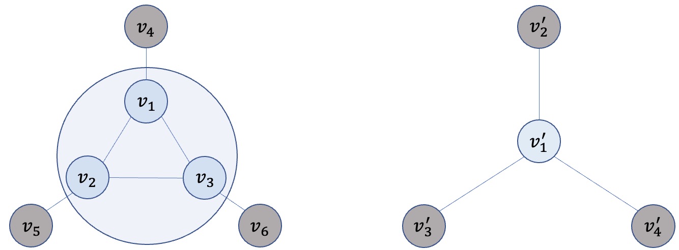
Graph coarsening is a methodology for solving large-scale graph problems. Depending on the problem itself, one may develop a solution based on the coarsened graph, or interpolate the solution back to the original one. Figure 1 illustrates a toy example of graph coarsening, whereby a cluster of nodes (, , and ) in the original graph are merged to a so-called supernode () in the coarsened graph. If the problem is graph classification (predicting classes of multiple graphs in a dataset), one may train a classifier by using these smaller surrogates, if it is believed that they inherit the characteristics of the original graphs necessary for classification. On the other hand, if the problem is node regression,111Machine learning problems on graphs could be on the graph level (e.g., classifying the toxicity of a protein graph) or on the node level (e.g., predicting the coordinates of each node (atom) in a molecular graph). In this work, our experiments focus on graph-level problems. one may predict the targets for the nodes in the coarsened graph and interpolate them in the original graph (Huang et al., 2021).
Graph coarsening has a long history in scientific computing, while it gains attraction in machine learning recently (Chen et al., 2022). A key question to consider is what characteristics should be preserved when reducing the graph size. A majority of work in machine learning focuses on the spectral properties (Loukas & Vandergheynst, 2018; Loukas, 2019; Hermsdorff & Gunderson, 2019; Jin et al., 2020). That is, one desires that the eigenvalues of the original graph are close to those of the coarsened graph . While being attractive, it is unclear why this objective is effective for problems involving a collection of graphs (e.g., graph classification), where the distances between graphs shape the classifier and the decision boundary. Hence, in this work, we consider a different objective, which desires that the distance of a pair of graphs, , is close to that of their coarsened versions, .
To achieve so, we make the following contributions.
-
•
We consider a graph as an element on the metric space endowed with the Gromov–Wasserstein (GW) distance (Chowdhury & Mémoli, 2019), which formalizes the distance of graphs with different sizes and different node weights. We analyze the distance between and as a major lemma for subsequent results.
-
•
We establish an upper bound on the difference of the GW distance between the original graph pair and that of the coarsened pair. Interestingly, this bound depends on only the respective spectrum change of each of the original graphs. Such a finding explains the effectiveness of spectrum-preserving coarsening methods for graph classification and regression problems.
-
•
We bridge the connection between the upper bound and weighted kernel -means, a popular clustering method, under a proper choice of the kernel. This connection leads to a graph coarsening method that we demonstrate to exhibit attractive inference qualities for graph-level tasks, compared with other spectrum-preserving methods.
2 Related Work
Graph coarsening was made popular by scientific computing many decades ago, where a major problem was to solve large, sparse linear systems of equations (Saad, 2003). (Geometric) Multigrid methods (Briggs et al., 2000) were used to solve partial differential equations, the discretization of which leads to a mesh and an associated linear system. Multigrid methods solve a smaller system on the coarsened mesh and interpolate the solution back to the original mesh. When the linear system is not associated with a geometric mesh, algebraic multigrid methods (Ruge & Stüben, 1987) were developed to treat the coefficient matrix as a general graph, so that graph coarsening results in a smaller graph and the procedure of “solving a smaller problem then interpolating the solution on the larger one” remains applicable.
Graph coarsening was introduced to machine learning as a methodology of graph summarization (Liu et al., 2018) through the concepts of “graph cuts,” “graph clustering,” and “graph partitioning.” A commonality of these concepts is that graph nodes are grouped together based on a certain objective. Graph coarsening plays an important role in multilevel graph partitioning (Karypis & Kumar, 1999). The normalized cut (Shi & Malik, 2000) is a well-known and pioneering method for segmenting an image treated as a graph. Dhillon et al. (2007) compute weighted graph cuts by performing clustering on the coarsest graph resulting from hierarchical coarsening and refining the clustering along the reverse hierarchy. Graph partitioning is used to form convolutional features in graph neural networks (Defferrard et al., 2016) and to perform neighborhood pooling (Ying et al., 2018). Graph coarsening is used to learn node embeddings in a hierarchical manner (Chen et al., 2018). For a survey of graph coarsening with comprehensive accounts on scientific computing and machine learning, see Chen et al. (2022).
A class of graph coarsening methods aim to preserve the spectra of the original graphs. Loukas & Vandergheynst (2018) and Loukas (2019) introduce the notion of “restricted spectral similarity” (RSS), requiring the eigenvalues and eigenvectors of the coarsened graph Laplacian, when restricted to the principal eigen-subspace, to approximate those of the original graph. Local variation algorithms are developed therein to achieve RSS. Jin et al. (2020) suggest the use of a spectral distance as the key metric for measuring the preservation of spectral properties. The authors develop two coarsening algorithms to maximally reduce the spectral distance between the original and the coarsened graph. Hermsdorff & Gunderson (2019) develop a probabilistic algorithm to coarsen a graph while preserving the Laplacian pseudoinverse, by using an unbiased procedure to minimize the variance.
Graph coarsening is increasingly used in deep learning. One limitation of traditional coarsening methods is that they mean to be universally applicable to any graphs, without the flexibility of adapting to a particular dataset or distribution of its own characteristics. Cai et al. (2021) address this limitation by adjusting the edge weights in the coarsened graph through graph neural networks (GNNs). Conversely, graph coarsening techniques can be applied to scale up GNNs by preprocessing the graphs (Huang et al., 2021). On a separate note, graph condensation (Jin et al., 2021) is another technique to accelerate GNNs, which uses supervised learning to condense node features and the graph structure. Furthermore, graph pooling can assign a node in the original graph to multiple supernodes (Grattarola et al., 2022), similar to the relaxation-based graph coarsening strategy explored in the algebraic multigrid literautre (Ron et al., 2011).
3 Notations and Preliminaries
In this section, we set up the notations for graph coarsening and review the background of Gromov–Wasserstein distance. Additional information can be found in Appendix A.
3.1 Graphs and Laplacians
We denote an undirected graph as , whose node set is with size and whose symmetric weighted adjacency is . The -by- (combinatorial) Laplacian matrix is defined as , where is the degree matrix. The normalized Lapalcian is . Without loss of generality, we assume that is connected, in which case the smallest eigenvalue of and is zero and is simple.
3.2 Graph coarsening and coarsened graphs
Given a graph , graph coarsening amounts to finding a smaller graph with nodes to approximate . One common coarsening approach obtains the coarsened graph from a parititioning of the node set (Loukas & Vandergheynst, 2018). In this approach, each subset of nodes are collapsed to a supernode in the coarsened graph and the edge weight between two supernodes is the sum of the edge weights crossing the two corresponding partitions. Additionally, the sum of the edge weights in a partition becomes the weight of the supernode. In the matrix notation, we use to denote the membership matrix induced by the partitioning , with the entry being , where is the indicator function. For notational convenience, we define the adjacency matrix of the coarsened graph to be . Note that includes not only edge weights but also node weights.
If we similarly define to be the degree matrix of the coarsened graph , then it can be verified that the matrix is a (combinatorial) Laplacian (because its smallest eigenvalue is zero and is simple). Additionally, is the normalized Laplacian.
In the literature, the objective of coarsening is often to minimize some difference between the original and the coarsened graph. For example, in spectral graph coarsening, Loukas (2019) proposes that the -norm of any -dimensional vector be close to the -norm of the -dimensional vector ; while Jin et al. (2020) propose to minimize the difference between the ordered eigenvalues of the Laplacian of and those of the lifted Laplacian of (such that the number of eigenvalues matches). Such objectives, while being natural and interesting in their own right, are not the only choice. Questions may be raised; for example, it is unclear why the objective is to preserve the Laplacian spectrum but not the degree distribution or the clustering coefficients. Moreover, it is unclear how preserving the spectrum benefits the downstream use. In this paper, we consider a different objective—preserving the graph distance—which may help, for example, maintain the decision boundary in graph classification problems. To this end, we review the Gromov–Wasserstein (GW) distance.
3.3 Gromov–Wasserstein distance and its induced metric space
The GW distance was originally proposed by Mémoli (2011) to measure the distance between two metric measure spaces and .222A metric measure space is the triple , where is a metric space with metric and is a Borel probability measure on . However, using metrics to characterize the difference between elements in sets and can be too restrictive. Peyré et al. (2016) relaxed the metric notion by proposing the GW discrepancy, which uses dissimilarity, instead of metric, to characterize differences. Chowdhury & Mémoli (2019) then extended the concept of GW distance/discrepancy from metric measure spaces to measure networks, which can be considered a generalization of graphs.
Definition 3.1 (Measure network).
A measure network is a triple , where is a Polish space (a separable and completely metrizable topological space), is a fully supported Borel probability measure, and is a bounded measurable function on .
In particular, a graph (augmented with additional information) can be taken as a discrete measure network. We let be the set of graph nodes and associate with it a probability mass , . Additionally, we associate with the node similarity matrix , whose entries are induced from the measurable map : . Note that the mass and the similarity do not necessarily need to be related to the node weights and edge weights, although later we will justify and advocate the use of some variant of the graph Lapalcian as .
For a source graph with nodes and mass and a target graph with nodes and mass , we can define a transport matrix , where specifies the probability mass transported from (the -th node of ) to (the -th node of ). We denote the collection of all feasible transport matrices as , which includes all that satisfy and . Using the transportation cost , Chowdhury & Mémoli (2019) define the distance for graphs as
| (1) |
whre the cross-graph dissimilarity matrix has entries (which by themselves are dependent on ).
The computation of the distance (GW distance for short) can be thought of as finding a proper alignment of nodes in two graphs, such that the aligned nodes and have similar interactions with other nodes in their respective graphs. Intuitively, this is achieved by assigning large transport mass to a node pair with small dissimilarity , making the GW distance a useful tool for graph matching (Xu et al., 2019b). We note that variants of the GW distance exist; for example, Titouan et al. (2019) proposed a fused GW distance by additioanlly taking into account the dissimilarity of node features. We also note that computing the GW distance is NP-hard, but several approximate methods were developed (Xu et al., 2019a; Zheng et al., 2022). In this work, we use the GW distance as a theoretical tool and may not need to compute it in action.
On closing this section, we remark that Chowdhury & Mémoli (2019, Theorem 18) show that the GW distance is indeed a metric for measure networks, modulo weak isomorphism.333The weak isomorphism allows a node to be split into several identical nodes with the mass preserved. See Definition 3 of Chowdhury & Mémoli (2019). Therefore, we can formally establish the metric space of interest.
Definition 3.2 ( space).
Let be the collection of all measure networks. For , we denote by the metric space of measure networks endowed with the distance defined in (3.3) and call it the space.
4 Graph Coarsening from a Gromov–Wasserstein Geometric View
In this section, we examine how the GW geometric perspective can shape graph coarsening. In Section 4.1, we provide a framework that unifies many variants of the coarsening matrices through the use of the probability mass introduced in the context of measure networks. Then, in Section 4.2, we analyze the variant associated with the similarity matrix . In particular, we establish an upper bound of the difference of the GW distances before and after coarsening. Based on the upper bound, in Section 4.3 we connect it with some spectral graph techniques and in Section 4.4 we advocate a choice of in practice.
4.1 A unified framework for coarsening matrices
The membership matrix is a kind of coarsening matrices: it connects the adjacency matrix with the coarsened version through . There are, however, different variants of coarsening matrices. We consider three here, all having a size .
-
(i)
Accumulation. This is the matrix . When multiplied to the left of , the -th row of the product is the sum of all rows of corresponding to the partition .
-
(ii)
Averaging. A natural alternative to summation is (weighted) averaging. We define the diagonal mass matrix and for each partition , the accumulated mass for all . Then, the averaging coarsening matrix is
This matrix takes the effect of averaging because of the division over . Moreover, when the probability mass is uniform (i.e., all ’s are the same), we have the relation .
-
(iii)
Projection. Neither nor is orthogonal. We define the projection coarsening matrix as
by noting that is the identity and hence has orthonoral rows. Therefore, the -by- matrix is a projection operator.
In Section 3.2, we have seen that the combinatorial Laplacian takes as the coarsening matrix, because the relationship inherits from . On the other hand, it can be proved that, if we take the diagonal mass matrix to be the degree matrix , the normalized Laplacian defined in Section 3.2 can be written as (see Section B.1). In other words, the normalized Laplacian uses as the coarsening matrix. The matrix is called a doubly-weighted Laplacian (Chung & Langlands, 1996).
For a general similarity matrix (not necessarily a Laplacian), we use the averaging coarsening matrix and define . This definition appears to be more natural in the GW setting; see a toy example in Section B.2. It is interesting to note that Vincent-Cuaz et al. (2022) proposed the concept of semi-relaxed GW (srGW) divergence, wherein the first-order optimality condition of the constrained srGW barycenter problem is exactly the equality . See Section B.3.
In the next subsection, we will consider the matrix . We define the coarsened version by using the projection coarsening matrix as in . We will bound the distance of the original and the coarsened graph by using the eigenvalues of and . The reason why and use different coarsening matrices lies in the technical subtlety of : absorbs this factor from .
4.2 Graph distance on the space
Now we consider the GW distance between two graphs. For theoretical and computational convenience, we take the transportation cost (i.e., taking in (3.3)). When two graphs and are concerned, we inherit the subscripts 1 and 2 to all related quantities, such as the probability masses and , avoiding verbatim redundancy when introducing notations. This pair of subscripts should not cause confusion with other subscripts, when interpreted in the proper context. Our analysis can be generalized from the distance to other distances, as long as the transportation cost satisfies the following decomposable condition.
Proposition 4.1.
(Peyré et al., 2016) Let be the optimal transport plan from to ,444The existence of is guaranteed by the fact that the feasible region of is compact and the object function is continuous with respect to . and be similarity matrices for . If the transport cost can be written as for some element-wise functions , then we can write in (3.3) as
Clearly, for the squared cost , we may take , , , and .
We start the analysis by first bounding the distance between and .
Theorem 4.2 (Single graph).
Consider a graph with positive semi-definite (PSD) similarity matrix and diagonal mass matrix and similarly the coarsened graph . Let be the sorted eigenvalues of and be the sorted eigenvalues of . Then,
| (2) |
where is non-negative and is independent of coarsening.
Remark 4.3.
(i) The bound is tight when because the right-hand side is zero in this case. (ii) The choice of coarsening only affects the spectral difference
| (3) |
because is independent of it. Each term in is non-negative due to the Poincaré separation theorem (see Section D.1). (iii) is a generalization of the spectral distance proposed by Jin et al. (2020), because our matrix is not necessarily the normalized Laplacian. For additional discussions, see Section B.4. (iv) When is taken as the normalized Laplacian, our bound is advantageous over the bound established by Jin et al. (2020) in the sense that is the only term impacted by coarsening and that no assumptions on the -means cost are imposed.
We now bound the difference of distances. The following theorem suggests that the only terms dependent on coarsening are and , counterparts of in Theorem 4.2, for graphs and respectively.
Theorem 4.4.
Given a pair of graphs and , we extend all notations in Theorem 4.2 by adding subscripts 1 and 2 respectively for and . We denote the optimal transport plan induced by as and let the normalized counterpart be . Additionally, we define with eigenvalues and with eigenvalues , both independent of coarsening. Then, is upper bounded by
where is from Theorem 4.2 and the other coarsening-independent terms are introduced in Lemma E.5 in Appendix E.
Remark 4.5.
(i) The above bound takes into account both the differences between two graphs and their respective coarsenings. Even when the two graphs are identical , the bound can still be nonzero if the coarsened graphs and do not match. (ii) The decoupling of and offers an algorithmic benefit when one wants to optimize the differences of distances for all graph pairs in a dataset: it suffices to optimize the distance between and for each graph individually. This benefit is in line with the prior practice of directly applying spectrum-preserving coarsening methods for graph-level tasks (Jin et al., 2020; Huang et al., 2021). Their experimental results and our numerical verification in Section 6 show that our bound is useful and it partly explains the empirical success of spectral graph coarsening.
4.3 Connections with truncated SVDs and Laplacian eigenmaps
The spectral difference in Theorem 4.2 can be used as the loss function for defining an optimal coarsening. Because and because is independent of coarsening, minimizing is equivalent to the following problem
| (4) |
by recalling that is a projector. The problem (4) is a well-known trace optimization problem, which has rich connections with many spectral graph techniques (Kokiopoulou et al., 2011).
Connection with truncated SVD. At first sight, a small trace difference does not necessarily imply the two matrices are close. However, because is a projector, the Poincaré separation theorem (see Section D.1) suggests that their eigenvalues can be close. A well-known example of using the trace to find optimal approximations is the truncated SVD, which retains the top singular values (equivalently eigenvalues for PSD matrices). The truncated SVD is a technique to find the optimal rank- approximation of a general matrix in terms of the spectral norm or the Frobenius norm, solving the problem
where is the class of all rank- orthogonal matrices. The projection coarsening matrix belongs to this class.
Connection with Laplacian eigenmaps. The Laplacian eigenmap (Belkin & Niyogi, 2003) is a manifold learning technique that learns an -dimensional embedding for points connected by a graph. The embedding matrix solves the trace problem . If we let , the problem is equivalent to
Different from truncated SVD, which uses the top singular vectors (eigenvectors) to form the solution, the Laplacian eigenmap uses the bottom eigenvectors of to form the solution.
4.4 Signless Laplacians as similarity matrices
The theory established in Section 4.2 is applicable to any PSD matrix , but for practical uses we still have to define it. Based on the foregoing exposition, it is tempting to let be the Laplacian or the normalized Laplacian , because they are PSD and they reveal important information of the graph structure (Tsitsulin et al., 2018). In fact, as a real example, Chowdhury & Needham (2021) used the heat kernel as the similarity matrix to define the GW distance (and in this case the GW framework is related to spectral clustering). However, there are two problems that make such a choice troublesome. First, the (normalized) Laplacian is sparse but its off-diagonal, nonzero entries are negative. Thus, when is interpreted as a similarity matrix, a pair of nodes not connected by an edge becomes more similar than a pair of connected nodes, causing a dilema. Second, under the trace optimization framework, one is lured to intuitively look for solutions toward the bottom eigenvectors of , like in Laplacian eigenmaps, an opposite direction to the true solution of (4), which is toward the top eigenvectors instead.
To resolve these problems, we propose to use the signless Laplacian (Cvetković et al., 2007), , or its normalized version, , as the similarity matrix . These matrices are PSD and their nonzero entries are all positive. With such a choice, the spectral difference in (3) has a fundamentally different behavior from the spectral distance used by Jin et al. (2020) when defining the coarsening objective.
5 Computational Equivalence between Graph Coarsening and Weighted Kernel -means
By recalling that and that is a projector, we rewrite the coarsening objective in (4) as
| (5) |
When is PSD, it could be interpreted as a kernel matrix such that there exists a set of feature vectors for which for . Then, with simple algebraic manipulation, we see that (5) is equivalent to the well-known clustering objective:
| (6) |
where the norm is induced by the inner product . Here, is the weighted center of for all nodes belonging to cluster . Hence, the weighted kernel -means algorithm (Dhillon et al., 2004, 2007) can be applied to minimize (6) by iteratively recomputing the centers and updating cluster assignments according to the distance of a node to all centers. We denote the squared distance between and any by , which is
| (7) |
The -means algorithm is summarized in Algorithm 1 and we call this method kernel graph coarsening (KGC).
Input: : similarity matrix, : node mass vector, : number of clusters
Output: : node partition
KGC as a post-refinement of graph coarsening. KGC can be used as a standalone coarsening method. A potential drawback of this usage is that the -means algorithm is subject to initialization and the clustering quality varies significantly sometimes. Even advanced initialization techniques, such as -means++ (Arthur & Vassilvitskii, 2006), are not gauranteed to work well in practice. Moreover, KGC, in the vanilla form, does not fully utilize the graph information (such as node features), unless additional engineering of the similarity matrix is conducted. Faced with these drawbacks, we suggest a simple alternative: initialize KGC by the output of another coarsening method and use KGC to improve it (Scrucca & Raftery, 2015). In our experience, KGC almost always monotonically reduces the spectral difference and improves the quality of the initial coarsening.
Time complexity. Let be the number of -means iterations. The time complexity of KGC is , where is the number of nonzeros in . See Section B.5 for the derivation of this cost and a comparison with the cost of spectral graph coarsening (Jin et al., 2020).
6 Numerical Experiments
We evaluate graph coarsening methods, including ours, on eight benchmark graph datasets: MUTAG (Debnath et al., 1991; Kriege & Mutzel, 2012), PTC (Helma et al., 2001), PROTEINS (Borgwardt et al., 2005; Schomburg et al., 2004), MSRC (Neumann et al., 2016), IMDB (Yanardag & Vishwanathan, 2015), Tumblr (Oettershagen et al., 2020), AQSOL (Sorkun et al., 2019; Dwivedi et al., 2020), and ZINC (Irwin et al., 2012). Information of these datasets is summarized in Table 1.
| Dataset | Classes | Size | ||
|---|---|---|---|---|
| MUTAG | 2 | 188 | 17.93 | 19.79 |
| PTC | 2 | 344 | 14.29 | 14.69 |
| PROTEINS | 2 | 1113 | 39.06 | 72.82 |
| MSRC | 8 | 221 | 39.31 | 77.35 |
| IMDB | 2 | 1000 | 19.77 | 96.53 |
| Tumblr | 2 | 373 | 53.11 | 199.78 |
| AQSOL | 9823 | 17.57 | 17.86 | |
| ZINC | 12000 | 23.16 | 49.83 | |
We compare our method with the following baseline methods (Loukas, 2019; Jin et al., 2020): Variation Neighborhood Graph Coarsening (VNGC); Variation Edge Graph Coarsening (VEGC); Multilevel Graph Coarsening (MGC); and Spectral Graph Coarsening (SGC). For our method, we consider the vanilla KGC, which uses -means++ for initialization, and the variant KGC(A), which takes the output of the best-performing baseline method for initialization. More implementation details are provided in Appendix C.
6.1 GW distance approximation
For a sanity check, we evaluate each coarsening method on the approximation of the GW distance, to support our motivation of minimizing the upper bound in Theorem 4.2.
We first compare the average squared GW distance, by using the normalized signless Laplacian as the similarity matrix (see Section 4.4). We vary the coarsened graph size for . For each graph in PTC and IMDB, we compute and report the average in Table 5, Appendix C.1. We obtain similar observations across the two datasets. In particular, KGC and KGC(A) outperform baselines. When is small, it is harder for -means clustering to find the best clustering plan and hence KGC(A) works better. When gets larger, KGC can work better, probably because the baseline outputs are poor intiializations.
We then report the average gap between the left- and right-hand sides of the bound (2) in Table 6, Appendix C.1. For all methods, including the baselines, the gap is comparable to the actual squared distance shown in Table 5, showcasing the quality of the bound. Moreover, the gap decreases when increases, as expected.
We next compute the matrix of GW distances, (before coarsening) and (after coarsening), and compute the change . Following previous works (Chan & Airoldi, 2014; Xu et al., 2020), we set . The similarity matrix for the coarsened graph uses the averaging coarsening matrix as advocated in Section 4.1; that is, . Additionally, we use a variant of the similarity matrix, , resulting from the projection coarsening matrix, for comparison.
| Coars. Mat. | Methods | Frob. Error | Time |
|---|---|---|---|
| Projection | VNGC | ||
| VEGC | |||
| MGC | |||
| SGC | |||
| Averaging | VNGC | ||
| VEGC | |||
| MGC | |||
| SGC | |||
| KGC | |||
| KGC(A) | |||
Table 2 summarizes the results for PTC. It confirms that using “Averaging” is better than using “Projection” for the coarsening matrix. Additionally, KGC(A) initialized with MGC (the best baseline) induces a significantly small change (though no better than the change caused by KGC), further verifying that minimizing the loss (4) will lead to a small change in the GW distance. The runtime reported in the table confirms the analysis in Section 5, showing that KGC is efficient. Moreover, the runtime of KGC(A) is nearly negligible compared with that of the baseline method used for initializing KGC(A).
6.2 Laplacian spectrum preservation
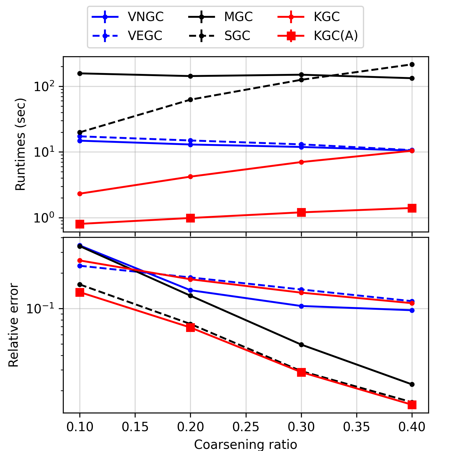
We evaluate the capability of the methods in preserving the Laplacian spectrum, by noting that the spectral objectives of the baseline methods differ from that of ours (see remarks after Theorem 4.2). We coarsen each graph to its , and size and evaluate the metric (the relative error of the first five largest eigenvalues). The experiment is conducted on Tumblr and the calculation of the error metric is repeated ten times.
In Figure 2, we see that KGC has a comparable error to the variational methods VNGC and VEGC, while incurring a lower time cost, especially when the coarsening ratio is small. Additionally, KGC(A) consistently improves the initialization method SGC and attains the lowest error.
| Datasets | MUTAG | PTC | PROTEINS | MSRC | IMDB | Tumblr |
|---|---|---|---|---|---|---|
| VNGC | ||||||
| VEGC | ||||||
| MGC | ||||||
| SGC | ||||||
| KGC | ||||||
| KGC(A) | ||||||
| EIG | ||||||
| FULL | ||||||
6.3 Graph classification using Laplacian spectrum
We test the performance of the various coarsening methods for graph classification. We follow the setting of Jin et al. (2020) and adopt the Network Laplacian Spectral Descriptor (Tsitsulin et al., 2018, NetLSD) along with a -NN classifier as the classification method. We set . For evaluation, we select the best average accuracy of 10-fold cross validations among three different seeds. Additionally, we add two baselines, EIG and FULL, which respectively use the first eigenvalues and the full spectrum of in NetLSD. Similarly to before, we initialize KGC(A) with the best baseline.
Table 3 shows that preserving the spectrum does not necessarily leads to the best classification, since EIG and FULL, which use the original spectrum, are sometime outperformed by other methods. On the other hand, our proposed method, KGC or KGC(A), is almost always the best.
6.4 Graph regression using GCNs
We follow the setting of Dwivedi et al. (2020) to perform graph regression on AQSOL and ZINC (see Appendix C.4 for details). For evaluation, we pre-coarsen the whole datasets, reduce the graph size by 70%, and run GCN on the coarsened graphs. Table 4 suggests that KGC(A) initialized with VEGC (the best baseline) always returns the best test MAE. On ZINC, KGC sometimes suffers from the initialization, but its performance is still comparable to a reported MLP baseline (Dwivedi et al., 2020, TestMAE ).
| Methods | TestMAEs.d. | TrainMAEs.d. | Epochs |
|---|---|---|---|
| VNGC | |||
| VEGC | |||
| MGC | |||
| SGC | |||
| KGC | |||
| KGC(A) | |||
| FULL | |||
| Methods | TestMAEs.d. | TrainMAEs.d. | Epochs |
|---|---|---|---|
| VNGC | |||
| VEGC | |||
| MGC | |||
| SGC | |||
| KGC | |||
| KGC(A) | |||
| FULL | |||
7 Conclusions
In this work, we propose a new perspective to study graph coarsening, by analyzing the distance of graphs on the GW space. We derive an upper bound on the change of the distance caused by coarsening, which depends on only the spectral difference . This bound in a way justifies the idea of preserving the spectral information as the main objective of graph coarsening, although our definition of “spectral-preserving” differs from prior spectral coarsening techniques. More importantly, we point out the equivalence between the bound and the objective of weighted kernel -means clustering. This equivalence leads to a new coarsening method we termed KGC. Our experiment results validate the theoretical analysis, showing that KGC preserves the GW distance between graphs and improves the accuracy of graph-level classification and regression tasks.
Acknowledgements
We wish to appreciate all the constructive and insightful comments from the anonymous reviewers. Yun Yang’s research was supported in part by U.S. NSF grant DMS-2210717. Jie Chen acknowledges supports from the MIT-IBM Watson AI Lab.
References
- Arthur & Vassilvitskii (2006) Arthur, D. and Vassilvitskii, S. k-means++: The advantages of careful seeding. Technical report, Stanford, 2006.
- Belkin & Niyogi (2003) Belkin, M. and Niyogi, P. Laplacian eigenmaps for dimensionality reduction and data representation. Neural computation, 15(6):1373–1396, 2003.
- Bellman (1997) Bellman, R. Introduction to matrix analysis. SIAM, 1997.
- Borgwardt et al. (2005) Borgwardt, K. M., Ong, C. S., Schönauer, S., Vishwanathan, S., Smola, A. J., and Kriegel, H.-P. Protein function prediction via graph kernels. Bioinformatics, 21(suppl_1):i47–i56, 2005.
- Briggs et al. (2000) Briggs, W. L., Henson, V. E., and McCormick, S. F. A Multigrid Tutorial. Society for Industrial and Applied Mathematics, 2nd edition, 2000.
- Cai et al. (2021) Cai, C., Wang, D., and Wang, Y. Graph coarsening with neural networks. In 9th International Conference on Learning Representations, ICLR 2021, Virtual Event, Austria, May 3-7, 2021. OpenReview.net, 2021.
- Chan & Airoldi (2014) Chan, S. and Airoldi, E. A consistent histogram estimator for exchangeable graph models. In Xing, E. P. and Jebara, T. (eds.), Proceedings of the 31st International Conference on Machine Learning, volume 32 of Proceedings of Machine Learning Research, pp. 208–216, Bejing, China, 22–24 Jun 2014. PMLR. URL https://proceedings.mlr.press/v32/chan14.html.
- Chen et al. (2018) Chen, H., Perozzi, B., Hu, Y., and Skiena, S. HARP: Hierarchical representation learning for networks. In AAAI, 2018.
- Chen et al. (2022) Chen, J., Saad, Y., and Zhang, Z. Graph coarsening: from scientific computing to machine learning. SeMA Journal, 79(1):187–223, 2022.
- Chowdhury & Mémoli (2019) Chowdhury, S. and Mémoli, F. The gromov–wasserstein distance between networks and stable network invariants. Information and Inference: A Journal of the IMA, 8(4):757–787, 2019.
- Chowdhury & Needham (2021) Chowdhury, S. and Needham, T. Generalized spectral clustering via gromov-wasserstein learning. In International Conference on Artificial Intelligence and Statistics, pp. 712–720. PMLR, 2021.
- Chung & Langlands (1996) Chung, F. R. and Langlands, R. P. A combinatorial laplacian with vertex weights. journal of combinatorial theory, Series A, 75(2):316–327, 1996.
- Cvetković et al. (2007) Cvetković, D., Rowlinson, P., and Simić, S. K. Signless laplacians of finite graphs. Linear Algebra and its applications, 423(1):155–171, 2007.
- Debnath et al. (1991) Debnath, A. K., Lopez de Compadre, R. L., Debnath, G., Shusterman, A. J., and Hansch, C. Structure-activity relationship of mutagenic aromatic and heteroaromatic nitro compounds. correlation with molecular orbital energies and hydrophobicity. Journal of medicinal chemistry, 34(2):786–797, 1991.
- Defferrard et al. (2016) Defferrard, M., Bresson, X., and Vandergheynst, P. Convolutional neural networks on graphs with fast localized spectral filtering. In Advances in Neural Information Processing Systems 29: Annual Conference on Neural Information Processing Systems 2016, December 5-10, 2016, Barcelona, Spain, pp. 3837–3845, 2016.
- Dhillon et al. (2004) Dhillon, I. S., Guan, Y., and Kulis, B. Kernel k-means: spectral clustering and normalized cuts. In Proceedings of the tenth ACM SIGKDD international conference on Knowledge discovery and data mining, pp. 551–556, 2004.
- Dhillon et al. (2007) Dhillon, I. S., Guan, Y., and Kulis, B. Weighted graph cuts without eigenvectors a multilevel approach. IEEE transactions on pattern analysis and machine intelligence, 29(11):1944–1957, 2007.
- Dobson & Doig (2003) Dobson, P. D. and Doig, A. J. Distinguishing enzyme structures from non-enzymes without alignments. Journal of molecular biology, 330(4):771–783, 2003.
- Dwivedi et al. (2020) Dwivedi, V. P., Joshi, C. K., Luu, A. T., Laurent, T., Bengio, Y., and Bresson, X. Benchmarking graph neural networks. arXiv preprint arXiv:2003.00982, 2020.
- Flamary et al. (2021) Flamary, R., Courty, N., Gramfort, A., Alaya, M. Z., Boisbunon, A., Chambon, S., Chapel, L., Corenflos, A., Fatras, K., Fournier, N., Gautheron, L., Gayraud, N. T., Janati, H., Rakotomamonjy, A., Redko, I., Rolet, A., Schutz, A., Seguy, V., Sutherland, D. J., Tavenard, R., Tong, A., and Vayer, T. Pot: Python optimal transport. Journal of Machine Learning Research, 22(78):1–8, 2021. URL http://jmlr.org/papers/v22/20-451.html.
- Grattarola et al. (2022) Grattarola, D., Zambon, D., Bianchi, F. M., and Alippi, C. Understanding pooling in graph neural networks. IEEE Transactions on Neural Networks and Learning Systems, 2022.
- Helma et al. (2001) Helma, C., King, R. D., Kramer, S., and Srinivasan, A. The predictive toxicology challenge 2000–2001. Bioinformatics, 17(1):107–108, 2001.
- Hermsdorff & Gunderson (2019) Hermsdorff, G. B. and Gunderson, L. M. A unifying framework for spectrum-preserving graph sparsification and coarsening. In Advances in Neural Information Processing Systems 32: Annual Conference on Neural Information Processing Systems 2019, NeurIPS 2019, December 8-14, 2019, Vancouver, BC, Canada, pp. 7734–7745, 2019.
- Hu et al. (2020) Hu, W., Fey, M., Zitnik, M., Dong, Y., Ren, H., Liu, B., Catasta, M., and Leskovec, J. Open graph benchmark: Datasets for machine learning on graphs. Advances in neural information processing systems, 33:22118–22133, 2020.
- Huang et al. (2021) Huang, Z., Zhang, S., Xi, C., Liu, T., and Zhou, M. Scaling up graph neural networks via graph coarsening. In Proceedings of the 27th ACM SIGKDD Conference on Knowledge Discovery & Data Mining, pp. 675–684, 2021.
- Irwin et al. (2012) Irwin, J. J., Sterling, T., Mysinger, M. M., Bolstad, E. S., and Coleman, R. G. Zinc: a free tool to discover chemistry for biology. Journal of chemical information and modeling, 52(7):1757–1768, 2012.
- Ivashkin & Chebotarev (2016) Ivashkin, V. and Chebotarev, P. Do logarithmic proximity measures outperform plain ones in graph clustering? In International Conference on Network Analysis, pp. 87–105. Springer, 2016.
- Jin et al. (2021) Jin, W., Zhao, L., Zhang, S., Liu, Y., Tang, J., and Shah, N. Graph condensation for graph neural networks. arXiv preprint arXiv:2110.07580, 2021.
- Jin et al. (2020) Jin, Y., Loukas, A., and JáJá, J. Graph coarsening with preserved spectral properties. In The 23rd International Conference on Artificial Intelligence and Statistics, AISTATS 2020, 26-28 August 2020, Online [Palermo, Sicily, Italy], volume 108 of Proceedings of Machine Learning Research, pp. 4452–4462. PMLR, 2020.
- Karypis & Kumar (1999) Karypis, G. and Kumar, V. A fast and high quality multilevel scheme for partitioning irregular graphs. SIAM Journal on Scientific Computing, 20(1):359–392, 1999.
- Kipf & Welling (2017) Kipf, T. N. and Welling, M. Semi-supervised classification with graph convolutional networks. In 5th International Conference on Learning Representations, ICLR 2017, Toulon, France, April 24-26, 2017, Conference Track Proceedings. OpenReview.net, 2017.
- Kokiopoulou et al. (2011) Kokiopoulou, E., Chen, J., and Saad, Y. Trace optimization and eigenproblems in dimension reduction methods. Numerical Linear Algebra with Applications, 18(3):565–602, 2011.
- Kriege & Mutzel (2012) Kriege, N. M. and Mutzel, P. Subgraph matching kernels for attributed graphs. In Proceedings of the 29th International Conference on Machine Learning, ICML 2012, Edinburgh, Scotland, UK, June 26 - July 1, 2012. icml.cc / Omnipress, 2012.
- Liu et al. (2018) Liu, Y., Safavi, T., Dighe, A., and Koutra, D. Graph summarization methods and applications: A survey. ACM Comput. Surv., 51(3), jun 2018. ISSN 0360-0300. doi: 10.1145/3186727. URL https://doi.org/10.1145/3186727.
- Loukas (2019) Loukas, A. Graph reduction with spectral and cut guarantees. Journal of Machine Learning Research, 20(116):1–42, 2019.
- Loukas & Vandergheynst (2018) Loukas, A. and Vandergheynst, P. Spectrally approximating large graphs with smaller graphs. In Proceedings of the 35th International Conference on Machine Learning, ICML 2018, Stockholmsmässan, Stockholm, Sweden, July 10-15, 2018, volume 80 of Proceedings of Machine Learning Research, pp. 3243–3252. PMLR, 2018.
- Mémoli (2011) Mémoli, F. Gromov–wasserstein distances and the metric approach to object matching. Foundations of computational mathematics, 11(4):417–487, 2011.
- Minka (2000) Minka, T. P. Old and new matrix algebra useful for statistics, 2000. https://tminka.github.io/papers/matrix/.
- Morris et al. (2020) Morris, C., Kriege, N. M., Bause, F., Kersting, K., Mutzel, P., and Neumann, M. Tudataset: A collection of benchmark datasets for learning with graphs. In ICML 2020 Workshop on Graph Representation Learning and Beyond (GRL+ 2020), 2020.
- Neumann et al. (2016) Neumann, M., Garnett, R., Bauckhage, C., and Kersting, K. Propagation kernels: efficient graph kernels from propagated information. Machine Learning, 102(2):209–245, 2016.
- Oettershagen et al. (2020) Oettershagen, L., Kriege, N. M., Morris, C., and Mutzel, P. Temporal graph kernels for classifying dissemination processes. In Proceedings of the 2020 SIAM International Conference on Data Mining, SDM 2020, Cincinnati, Ohio, USA, May 7-9, 2020, pp. 496–504. SIAM, 2020. doi: 10.1137/1.9781611976236.56.
- Peyré et al. (2016) Peyré, G., Cuturi, M., and Solomon, J. Gromov-wasserstein averaging of kernel and distance matrices. In Proceedings of the 33nd International Conference on Machine Learning, ICML 2016, New York City, NY, USA, June 19-24, 2016, volume 48 of JMLR Workshop and Conference Proceedings, pp. 2664–2672. JMLR.org, 2016.
- Ron et al. (2011) Ron, D., Safro, I., and Brandt, A. Relaxation-based coarsening and multiscale graph organization. Multiscale Modeling & Simulation, 9(1):407–423, 2011.
- Ruge & Stüben (1987) Ruge, J. W. and Stüben, K. Algebraic multigrid. In Multigrid methods, pp. 73–130. SIAM, 1987.
- Ruhe (1970) Ruhe, A. Perturbation bounds for means of eigenvalues and invariant subspaces. BIT Numerical Mathematics, 10(3):343–354, 1970.
- Saad (2003) Saad, Y. Iterative Methods for Sparse Linear Systems. Society for Industrial and Applied Mathematics, 2nd edition, 2003.
- Schomburg et al. (2004) Schomburg, I., Chang, A., Ebeling, C., Gremse, M., Heldt, C., Huhn, G., and Schomburg, D. Brenda, the enzyme database: updates and major new developments. Nucleic acids research, 32(suppl_1):D431–D433, 2004.
- Scrucca & Raftery (2015) Scrucca, L. and Raftery, A. E. Improved initialisation of model-based clustering using gaussian hierarchical partitions. Advances in data analysis and classification, 9(4):447–460, 2015.
- Shi & Malik (2000) Shi, J. and Malik, J. Normalized cuts and image segmentation. IEEE Transactions on pattern analysis and machine intelligence, 22(8):888–905, 2000.
- Sorkun et al. (2019) Sorkun, M. C., Khetan, A., and Er, S. Aqsoldb, a curated reference set of aqueous solubility and 2d descriptors for a diverse set of compounds. Scientific data, 6(1):1–8, 2019.
- Titouan et al. (2019) Titouan, V., Courty, N., Tavenard, R., and Flamary, R. Optimal transport for structured data with application on graphs. In International Conference on Machine Learning, pp. 6275–6284. PMLR, 2019.
- Tsitsulin et al. (2018) Tsitsulin, A., Mottin, D., Karras, P., Bronstein, A. M., and Müller, E. Netlsd: Hearing the shape of a graph. In Proceedings of the 24th ACM SIGKDD International Conference on Knowledge Discovery & Data Mining, KDD 2018, London, UK, August 19-23, 2018, pp. 2347–2356. ACM, 2018. doi: 10.1145/3219819.3219991.
- Vincent-Cuaz et al. (2022) Vincent-Cuaz, C., Flamary, R., Corneli, M., Vayer, T., and Courty, N. Semi-relaxed gromov-wasserstein divergence and applications on graphs. In International Conference on Learning Representations, 2022. URL https://openreview.net/forum?id=RShaMexjc-x.
- Xu et al. (2019a) Xu, H., Luo, D., and Carin, L. Scalable gromov-wasserstein learning for graph partitioning and matching. Advances in neural information processing systems, 32, 2019a.
- Xu et al. (2019b) Xu, H., Luo, D., Zha, H., and Carin, L. Gromov-wasserstein learning for graph matching and node embedding. In Proceedings of the 36th International Conference on Machine Learning, ICML 2019, 9-15 June 2019, Long Beach, California, USA, volume 97 of Proceedings of Machine Learning Research, pp. 6932–6941. PMLR, 2019b.
- Xu et al. (2020) Xu, H., Luo, D., Carin, L., and Zha, H. Learning graphons via structured gromov-wasserstein barycenters. In AAAI Conference on Artificial Intelligence, 2020.
- Yanardag & Vishwanathan (2015) Yanardag, P. and Vishwanathan, S. V. N. Deep graph kernels. In Proceedings of the 21th ACM SIGKDD International Conference on Knowledge Discovery and Data Mining, Sydney, NSW, Australia, August 10-13, 2015, pp. 1365–1374. ACM, 2015. doi: 10.1145/2783258.2783417.
- Ying et al. (2018) Ying, R., You, J., Morris, C., Ren, X., Hamilton, W. L., and Leskovec, J. Hierarchical graph representation learning with differentiable pooling. In NeurIPS, 2018.
- Zheng et al. (2022) Zheng, L., Xiao, Y., and Niu, L. A brief survey on computational gromov-wasserstein distance. Procedia Computer Science, 199:697–702, 2022.
Appendix A List of notations
| Notations | Meaning |
|---|---|
| (coarsened) graph Laplacian matrix | |
| (coarsened) normalized graph Laplacian matrix | |
| coarsened graph | |
| (coarsened) degree matrix | |
| (coarsened) adjacency matrix | |
| membership matrix, coarsening matrix with entries | |
| orthogonal coarsening matrix, a variant of coarsening matrix | |
| weighted averaging matrix, a variant of coarsening matrix | |
| projection matrix induced by | |
| diagonal node mass matrix | |
| () | (coarsened) similarity matrix |
We elaborate more about the family of coarsening matrices here. Specifically, we define the matrix as
Let be the number of nodes in the -th partition and be the number of partitioning. Then, we define the weight matrix and let . We can thus give the definition of the weighted averaging matrix as
and the orthogonal coarsening matrix
Let the projection matrix be . We can check that .
Appendix B Derivations Omitted in the Main Text
B.1 Weighted graph coarsening leads to doubly-weighted Laplacian
We show in the following that can reproduce the normalized graph Laplacian . In this case, and interestingly , indicating
The results above imply we can unify previous coarsening results under the weighted graph coarsening framework in this paper, with a proper choice of similarity matrix and node measure .
B.2 A toy example of coarsening a 3-node graph
Consider a fully-connected 3-node graph with equal weights for nodes and the partition . Its similarity matrix and the three possible coarsened similarity matrices will respectively be
It is clear that , which will have the most appropriate entry magnitude to give the minimal GW-distance, is different from proposed in Jin et al. (2020) and (Cai et al., 2021). We note in the edge weight (similarity) is still 1, since we explicitly specify the node weight of the supernode becomes . The new GW geometric framework thus decouples the node weights and similarity intensities.
B.3 Deriving the “Averaging” magnitude from the constrained srGW barycenter problem
We first introduce the definition of srGW divergence. For a given graph with node mass distribution and similarity matrix , we can construct another graph with given similarity matrix and unspecified node mass distribution . To better reflect the dependence of on node mass distribution and similarity matrix, we abuse the notation as and in this subsection. Vincent-Cuaz et al. (2022) then defined
and we can further find an optimal (w.r.t. the srGW divergence) by solving the following srGW barycenter problem with only one input , i.e.
| (8) |
We can then do the following transform to Equation 8 to reveal its connection with our proposed “Averaging” magnitude for the coarsened similarity matrix .
In the display above, we use and to show the dependence terms of the cross-graph dissimilarity matrix and the transport matrix . The last equation holds since for a given transport matrix the new node mass distribution is uniquely decided by .
Notably, there is a closed-form solution for the inner minimization problem . Peyré et al. (2016, Equation (14)) derive that the optimal reads
If we then enforce the restriction that the node mass transport must be performed in a clustering manner (i.e., the transport matrix for a certain membership matrix ), we exactly have . The derivation above verifies the effectiveness of the “Averaging” magnitude we propose.
B.4 Comparing spectral difference to spectral distance in Jin et al. (2020)
Jin et al. (2020) proposed to specify the graph coarsening plan by minimizing the following full spectral distance term (c.f. their Equation (8)):
where ’s and ’s correspond to the eigenvalues (in an ascending order) of the normalized Laplacian and , and and are defined as . The last equation holds due to their Interlacing Property 4.1 (similar to Theorem D.1).
We note (i) the two “spectral” loss functions, and , refer to different spectra. We leverage the spectrum of while they focus on graph Laplacians. Our framework is more general and takes node weights into consideration. (ii) They actually divided ’s into two sets and respectively compared them to and ; the signs for and are thus different.
B.5 Time complexity of Algorithm 1
We first recall the complexity of Algorithm 1 stated in Section 5. Let be the upper bound of the -means iteration, the time complexity of Algorithm 1 is , where is the number of non-zero elements in .
The cost mainly comes from the computation of the “distance” (7), which takes time to obtain the second term in Equation 7 and pre-compute the third term (independent of ); obtaining the exact for all the pairs requires another time. Compared to the previous spectral graph coarsening method (Jin et al., 2020), Algorithm 1 removes the partial sparse eigenvalue decomposition, which takes time using Lanczos iteration with restarts. The -means part of spectral graph coarsening takes for a certain choice of the eigenvector feature dimension (Jin et al., 2020, Section 5.2), while weighted kernel -means clustering nested in our algorithm can better utilize the sparsity in the similarity matrix.
Appendix C Details of Experiments
We first introduce the hardware and the codebases we utilize in the experiments. The algorithms tested are all implemented in unoptimized Python code, and run with one core of a server CPU (Intel(R) Xeon(R) Gold 6240R CPU @ 2.40GHz) on Ubuntu 18.04. Specifically, our method KGC is developed based on the (unweighted) kernel -means clustering program provided by Ivashkin & Chebotarev (2016); for the other baseline methods, the variation methods VNGC and VEGC are implemented by Loukas (2019), and the spectrum-preserving methods MGC and SGC are implemented by Jin et al. (2020); The S-GWL method (Xu et al., 2019a; Chowdhury & Needham, 2021) is tested as well (can be found in the GitHub repository of this work), while this algorithm cannot guarantee that the number of output partition is the same as specified. For the codebases, we implement the experiments mainly using the code by Jin et al. (2020); Dwivedi et al. (2020), for graph classification and graph regression respectively. More omitted experimental settings in Section 6 will be introduced along the following subsections.
| Dataset | Methods | ||||
|---|---|---|---|---|---|
| PTC | VNGC | 0.05558 | 0.04880 | 0.03781 | 0.03326 |
| VEGC | 0.03064 | 0.02352 | 0.01614 | 0.00927 | |
| MGC | 0.05290 | 0.04360 | 0.02635 | 0.00598 | |
| SGC | 0.03886 | 0.03396 | 0.02309 | 0.00584 | |
| KGC | 0.03332 | 0.02369 | 0.01255 | 0.00282 | |
| KGC(A) | 0.03055 | 0.02346 | 0.01609 | 0.00392 | |
| IMDB | VNGC | 0.05139 | 0.05059 | 0.05043 | 0.05042 |
| VEGC | 0.02791 | 0.02106 | 0.01170 | 0.00339 | |
| MGC | 0.02748 | 0.02116 | 0.01175 | 0.00339 | |
| SGC | 0.02907 | 0.02200 | 0.01212 | 0.00352 | |
| KGC | 0.02873 | 0.02111 | 0.01137 | 0.00320 | |
| KGC(A) | 0.02748 | 0.02106 | 0.01170 | 0.00337 | |
C.1 Details of GW distance approximation in Section 6.1
| Dataset | Methods | ||||
|---|---|---|---|---|---|
| PTC | VNGC | 0.06701 | 0.06671 | 0.05393 | 0.04669 |
| VEGC | 0.06246 | 0.06129 | 0.04424 | 0.02577 | |
| MGC | 0.03203 | 0.03200 | 0.02167 | 0.00540 | |
| SGC | 0.04599 | 0.04156 | 0.02488 | 0.00554 | |
| KGC | 0.05145 | 0.05173 | 0.03530 | 0.00852 | |
| KGC(A) | 0.06519 | 0.06402 | 0.04702 | 0.00372 | |
| IMDB | VNGC | 0.009281 | 0.00927 | 0.009278 | 0.009268 |
| VEGC | 0.016879 | 0.016735 | 0.01636 | 0.008221 | |
| MGC | 0.017307 | 0.01663 | 0.016309 | 0.008179 | |
| SGC | 0.015719 | 0.015793 | 0.015934 | 0.008049 | |
| KGC | 0.016054 | 0.016679 | 0.016687 | 0.008347 | |
| KGC(A) | 0.017307 | 0.016735 | 0.01636 | 0.008177 | |
We compute the pair-wise distance matrix for graphs in PTC and IMDB, with the normalized signless Laplacians set as the similarity matrices. For the computation of the distance, we mainly turn to the popular OT package POT (Flamary et al., 2021, Python Optimal Transport).
The omitted tables of average squared GW distance and average empirical bound gaps are presented in Tables 5 and 6.
Regarding time efficiency, we additionally remark our method KGC works on the dense graph matrix, even though it has a better theoretical complexity using a sparse matrix; for small graphs in MUTAG, directly representing them by dense matrices would even be faster, when a modern CPU is used.
C.2 Details of Laplacian spectrum preservation in Section 6.2
C.3 Details of Graph classification with Laplacian spectrum in Section 6.3
C.4 Details of Graph regression with GCNs in Section 6.4
We mainly follow the GCN settings in Dwivedi et al. (2020). More detailed settings are stated as follows.
Graph regression. The procedure of graph regression is as follows: Taking a graph as input, a GCN will return a graph embedding ; Dwivedi et al. (2020) then pass to an MLP and compute the prediction score as
where . They will then use , the loss (the MAE metric in Table 4) between the predicted score and the groundtruth score , both in training and performance evaluation.
Data splitting. They apply a scaffold splitting (Hu et al., 2020) to the AQSOL dataset in the ratio to have , and samples for train, validation, and test sets.
Training hyperparameters. For the learning rate strategy across all GCN models, we follow the existing setting to choose the initial learning rate as , the reduce factor is set as , and the stopping learning rate is . Also, all the GCN models tested in our experiments share the same architecture—the network has layers and tunable parameters.
As for the concrete usage of graph coarsening to GCNs, we discuss the main idea in Section C.4.1 and leave the technical details to Section C.4.2.
C.4.1 Application of graph coarsening to GCNs
Motivated by the GW setting, we discuss the application of graph coarsening to a prevailing and fundamental graph model—GCN555We omit the introduction to GCN here and refer readers to Kipf & Welling (2017) for more details.. After removing the bias term for simplicity and adapting the notations in this paper, we take a vanilla -layer GCN as an example and formulate it as
where is the graph representation of a size- graph associated with the adjacency matrix , is an arbitrary activation function, is the embedding matrix for nodes in the graph, and is the weight matrix for the linear transform in the layer. We take the mean operation in the GCN as an implication of even node weights (therefore no subscript for coarsening matrices), and intuitively incorporate graph coarsening into the computation by solely replacing with and denote as the corresponding representation. We have
| (9) |
and the graph matrix is supposed to be coarsened as , which can be extended to multiple layers. Due to the space limit, we defer the derivation to Appendix C.4.2 and solely leave some remarks here.
The propagation above is guided by the GW setting along this paper: even the nodes in the original graph are equally-weighted, the supernodes after coarsening can have different weights, which induces the new readout operation ( is the mass vector of the supernodes). Furthermore, an obvious difference between Equation 9 and previous designs (Huang et al., 2021; Cai et al., 2021) of applying graph coarsening to GNNs is the asymmetry of the coarsened graph matrix . The design (9) is tested for the graph regression experiment in Section 6.4. More technical details are introduced in the subsequent subsection.
C.4.2 Derivation of the GCN propagation in the GW setting
We consider a general layer- GCN used by Dwivedi et al. (2020). We first recall the definition (normalization modules are omitted for simplicity):
where is an activation function and from now on we will abuse here to denote ; is the embedding matrix of the graph nodes in the -th layer, and is the weight matrix of the same layer.
To apply the coarsened graph, we enforce the following regulations:
To reduce the computation in node aggregation, we utilize the two properties that and , for any element-wise activation function and matrix with a proper shape (considering simply “copy” the rows from ); for the top two layers, we then have
Note ; for the top two layers we finally obtain
implying that we can replace with in the propagation of the top two layers. The trick can indeed be repeated for each layer, and specifically, in the bottom layer we can have
which well corresponds to the node weight concept in the GW setting: uses the average embedding of the nodes within the cluster to represent the coarsened centroid. We then finish the justification of the new GCN propagation in Equation 9.
Appendix D Useful Facts
D.1 Poincaré separation theorem
For convenience of the reader, we repeat Poincaré separation theorem (Bellman, 1997) in this subsection.
Theorem D.1 (Poincaré separation theorem).
Let be an real symmetric matrix and an semi-orthogonal matrix such that . Denote by and the eigenvalues of and , respectively (in descending order). We have
| (10) |
D.2 Ruhe’s trace inequality
For convenience of the reader, Ruhe’s trace inequality (Ruhe, 1970) is stated as follows.
Lemma D.2 (Ruhe’s trace inequality).
If are both PSD matrices with eigenvalues,
then
Appendix E Proof of Theorem 4.2 and Theorem 4.4
We will first prove an intermediate result Lemma E.1 for coarsened graph and un-coarsend graph to introduce necessary technical tools for Theorem 4.2 and Theorem 4.4. The ultimate proof of Theorem 4.2 and Theorem 4.4 will be stated in Appendix E.2 and Appendix E.3 respectively.
E.1 Lemma E.1 and Its Proof
We first give the complete statement of Lemma E.1. In Lemma E.1, we consider the case in which only graph is coarsened, and the notations are slightly simplified: when the context is clear, the coarsening-related terms without subscripts specific to graphs, e.g. , are by default associated with unless otherwise announced. We follow the simplified notation in the statement and proof of Theorem 4.2, which focuses on solely and the indices are not involved. For Theorem 4.4, we will explicitly use specific subscripts, such as , for disambiguation.
Lemma E.1.
Let . If both and are PSD, we have
| (11) | ||||
Here, are eigenvalues of , with eigenvalues , and with eigenvalues , and we let and be two non-negative constants.
Remark E.2.
To illustrate our idea more clearly, we will start from the following decomposition of distance. The detailed proofs of all the lemmas in this section will be provided to Appendix E.4 for the readers interested.
Lemma E.3.
For any two graphs and , we have
where
do not depend on the choice of transport map, while
requires the optimal transport map from the graph to the graph .
Replacing the -related terms in Equation 15 with their counterparts, we know that the distance between and is , where:
| (12) |
(co represents the transport from the “c”oarsened graph to the “o”riginal graph) here is the optimal transport matrix induced by the GW distance and .
The key step to preserve the GW distance is to control the difference and , since will cancel each other. We will start from the bound of .
Lemma E.4.
Let . If the similarity matrix is PSD, we have
Here, are the eigenvalues of , and is non-negative.
We can similarly bound with an additional tool Ruhe’s trace inequality (a variant of Von Neumann’s trace inequality specific to PSD matrices, c.f. Appendix D.2).
Lemma E.5.
Let be the normalized optimal transport matrix, and with eigenvalues . If both and are PSD, we have
Here, is non-negative.
Now we have
considering that and . Then, combining all the pieces above yields the bound in Lemma E.1.
E.2 Proof of Theorem 4.2
With the above dissection of the terms , we can now give a finer control of the distance . We first expand as
where the notation is now abused as the optimal transport matrix induced by . Applying the optimality inequality in Lemma E.7, we have
where we remark is a qualified transport matrix for and .
To further simplify the upper bound above, we show the equivalence between and as follows:
Combing the above pieces together, we obtain
which uses Lemma E.4 for the last inequality. The proof of Theorem 4.2 is now complete.
Remark E.6.
Theorem 4.2 can be leveraged to directly control . Note that is a pseudo-metric and satisfies triangular inequality (Chowdhury & Mémoli, 2019), which implies
and similarly we have
This implies
Here, the last inequality is due to Theorem 4.2. We comment the above result obtained from a direct application of triangle inequality is indeed weaker than the result stated in Theorem 4.4; we will then devote the remaining part of this section to the proof thereof.
E.3 Proof of Theorem 4.4
For one side of the result, we can follow the derivation in Lemma E.3 and apply Theorem 4.2 to have
where we recall and now is ( is the optimal transport matrix for and ).
For the other side, we still decompose the object as , and similarly we can follow Lemma E.4 to bound the first two terms. The next task is to disassemble .
We first prepare some notations for the analysis. To clarify the affiliation, we redefine with eigenvalues , with eigenvalues 666We index as since it is associated with and is an matrix., with eigenvalues , with eigenvalues , and similarly re-introduce , , and
Recalling Lemma E.7, we can analogously obtain ; replacing with , we have
where we apply the same derivation as in Equation (16) to obtain the second line above. For simplicity, we let and . We can now bound as
| (13) | ||||
E.4 Proof of some technical results
E.4.1 Proof of Lemma E.3
Proof.
Following the definition in Section 3.3, we rewrite the GW distance in the trace form and have
| (14) |
the third equation above holds because for any , and .
In the classical square loss case, we can immediately have and , where denotes the Hadamard product of two matrices with the same size. We can accordingly expand the first term in Equation 14 as
in which the proof of the last equation is provided in a summary sheet by Minka (2000). We note and is constructed symmetric; combining the pieces above we have
and similarly we obtain . The GW distance (14) can be therefore represented as
| (15) |
E.4.2 Proof of Lemma E.4
E.4.3 Proof of Lemma E.5
Proof.
By applying Lemma E.7, we have
Recall that are eigenvalues of , and let be eigenvalues of . Applying Ruhe’s trace inequality (c.f. Appendix D.2), we further have
| (18) |
(i) is by Ruhe’s trace inequality (Lemma D.2), since both and are PSD, and both (ii) and (iii) are by Poincaré separation theorem (Theorem D.1).
E.5 Other technical lemmas
Lemma E.7.
We have
Proof.
The proof is based on the optimality of , i.e. the GW distance induced by must be upper bounded by any other transport matrix. Intuitively, we can imagine the mass of a cluster center is transported to the same target nodes in as the original source nodes within this cluster, which corresponds to the transport matrix . We can verify is feasible, since and .
To derive the upper bound, applying the optimality of yields
| (19) | |||
| (20) | |||
| (21) | |||
| (22) |
The treatment is similar for the lower bound. We replace with . Then again due to the optimality of :
given our definition.
Remark. An intuitive scheme to control the upper bound (22) is to upper bound the trace of the -related matrix difference , since in coarsening we have no information about ; we will shortly showcase the term is the key to bound the whole GW distance difference as well.
Lemma E.8.
Consider a non-negative matrix in which all the elements . We keep to denote , and . Then we have .
Proof.
Motivated by the regular proof for bounding the eigenvalues of normalized Laplacian matrices, with two arbitrary vectors on the unit spheres we can recast the target statement as
| (23) |
We denote the diagonals for and respectively as and ; then we can rewrite the right-hand-side quantity in Inequality (23) as
where the second equation holds due to the conditions and , and the last inequality holds since .
Lemma E.9.
Consider a positive semi-definite (PSD) similarity matrix along with the probability mass vector and the diagonal matrix . For any non-overlapping partition , we denote the corresponding coarsening matrices and the projection matrix . Let . Then we have
| (24) |
Proof.
We first transform as follows:
and the last two equations hold due to .
We notice is symmetric and we can apply Poincaré separation theorem (c.f. Appendix D.1 for the complete statement) to control the eigenvalues of . Specifically, let be the eigenvalues of , and let be the eigenvalues of ; for all we have (being non-negative due to the PSD-ness of ); and a further conclusion . We can therefore complete the proof with .