A hierarchical decomposition for explaining ML performance discrepancies
Abstract
Machine learning (ML) algorithms can often differ in performance across domains. Understanding why their performance differs is crucial for determining what types of interventions (e.g., algorithmic or operational) are most effective at closing the performance gaps. Existing methods focus on aggregate decompositions of the total performance gap into the impact of a shift in the distribution of features versus the impact of a shift in the conditional distribution of the outcome ; however, such coarse explanations offer only a few options for how one can close the performance gap. Detailed variable-level decompositions that quantify the importance of each variable to each term in the aggregate decomposition can provide a much deeper understanding and suggest much more targeted interventions. However, existing methods assume knowledge of the full causal graph or make strong parametric assumptions. We introduce a nonparametric hierarchical framework that provides both aggregate and detailed decompositions for explaining why the performance of an ML algorithm differs across domains, without requiring causal knowledge. We derive debiased, computationally-efficient estimators, and statistical inference procedures for asymptotically valid confidence intervals.
1 Introduction
The performance of an ML algorithm can differ across domains due to shifts in the data distribution. To understand what contributed to this performance gap, prior works have suggested decomposing the gap into that due to a shift in the marginal distribution of the input features versus that due to a shift in the conditional distribution of the outcome (Cai et al., 2023; Zhang et al., 2023; Liu et al., 2023; Qiu et al., 2023; Firpo et al., 2018). Although such aggregate decompositions can be helpful, more detailed explanations that quantify the importance of each variable to each term in this decomposition can provide deeper insight to ML teams trying to understand and close the performance gap. However, there is currently no principled framework that provides both aggregate and detailed decompositions for explaining performance gaps of ML algorithms.
As a motivating example, suppose an ML deployment team has an algorithm that predicts the risk of patients being readmitted to the hospital given data from the Electronic Health Records (EHR), e.g. demographic variables and diagnosis codes. The algorithm was trained for a general patient population. The team intends to deploy it for heart failure (HF) patients and observes a large performance drop (e.g. in accuracy) in this subgroup. An aggregate decomposition of the performance drop into the marginal versus conditional components ( and ) provides only a high-level understanding of the underlying cause and limited suggestions on how the model can be fixed. A small conditional term in the aggregate decomposition but a large marginal term is typically addressed by retraining the model on a reweighted version of the original data that matches the target population (Quionero-Candela et al., 2009); otherwise, the standard suggestion is to collect more data from the target population to recalibrate/fine-tune the algorithm (Steyerberg, 2009). A detailed decomposition would help the deployment team conduct a root cause analysis and assess the utility of targeted variable-specific interventions. For instance, if the performance gap is primarily driven by a marginal shift in a few diagnoses, the team can investigate why the rates of these diagnoses differ between general and HF patients. The team may find that certain diagnoses differ due to variations in patient case mix, which may be better addressed through model retraining, whereas others are due to variations in documentation practices, which may be better addressed through operational interventions.
Existing approaches for providing a detailed understanding of why the performance of an ML algorithm differs across domains fall into two general categories. One category, which is also the most common in the applied literature, is to quantify how much the data distribution shifted (Liu et al., 2023; Budhathoki et al., 2021; Kulinski et al., 2020; Rabanser et al., 2019), e.g. one can compare how the distribution of each input variable differs across domains (Cummings et al., 2023). However, given the complex interactions and non-linearities in (black-box) ML algorithms, it is difficult to quantify how exactly such shifts contribute to changes in performance. For instance, a large shift with respect to a given variable does not necessarily translate to a large shift in model performance, as that variable may have low importance in the algorithm or the performance metric may be insensitive to that shift. Thus the other category of approaches—which is also the focus of this manuscript—is to directly quantify how a shift with respect to a variable (subset) influences model performance. Existing proposals only provide detailed variable-level breakdowns for either the marginal or conditional terms in the aggregate decomposition, but no unified framework exists. Moreover, existing methods either require knowledge of the causal graph relating all variables (Zhang et al., 2023) or strong parametric assumptions (Wu et al., 2021; Dodd & Pepe, 2003).
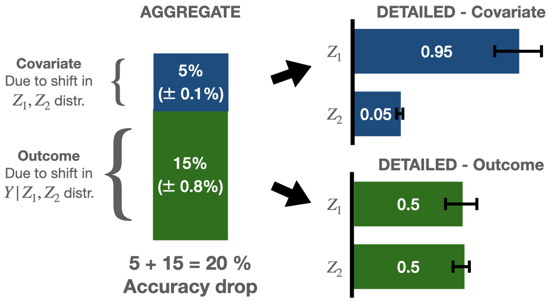
This work introduces a unified nonparametric framework for explaining the performance gap of an ML algorithm that first decomposes the gap into terms at the aggregate level and then provides detailed variable importance (VI) values for each aggregate term (Fig 1). Whereas prior works only provide point estimates for the decomposition, we derive debiased, asymptotically linear estimators for the terms in the decomposition which allow for the construction of confidence intervals (CIs) with asymptotically valid coverage rates. Uncertainty quantification is crucial in this setting, as one often has limited labeled data from the target domain. The estimation and statistical inference procedure is computationally efficient, despite the exponential number of terms in the Shapley value definition. We demonstrate the utility of our framework in real-world examples of prediction models for hospital readmission and insurance coverage.
2 Prior work
Describing distribution shifts. This line of work focuses on detecting and localizing which distributions shift between datasets (Kulinski et al., 2020; Rabanser et al., 2019). Budhathoki et al. (2021) identify the main variables contributing to a distribution shift via a Shapley framework, Kulinski & Inouye (2023) fits interpretable optimal transport maps, and Liu et al. (2023) finds the region with the largest shift in the conditional outcome distribution. However, these works do not quantify how these shifts contribute to changes in performance, the metric of practical importance.
Explaining loss differences across subpopulations. Understanding differences in model performance across subpopulations in a single dataset is similar to understanding differences in model performance across datasets, but the focus is typically to find subpopulations with poor performance rather than to explain how distribution shifts contributed to the performance change. Existing approaches include slice discovery methods (Plumb et al., 2023; Jain et al., 2023; d’Eon et al., 2022; Eyuboglu et al., 2022) and structured representations of the subpopulation using e.g. Euclidean balls (Ali et al., 2022).
Attributing performance changes. Prior works have described similar aggregate decompositions of the performance change into covariate and conditional outcome shift components (Cai et al., 2023; Qiu et al., 2023). To provide more granular explanations of performance shifts, existing works quantify the importance of shifts in each variable assuming the true causal graph is known (Zhang et al., 2023); covariate shifts restricted to variable subsets assuming partial shifts follow a particular structure (Wu et al., 2021); and conditional shifts in each variable assuming a parametric model (Dodd & Pepe, 2003). However, the strong assumptions made by these methods make them difficult to apply in practice, and model misspecification can lead to unintuitive interpretations. In addition, there is no unifying framework for decomposing both covariate and outcome shifts, and many methods do not output CIs, which is important when the amount of labeled data from a given domain is limited. A summary of how the proposed framework compares against prior works is shown in Table 1 of the Appendix.
Decomposition methods in econometrics. Explaining performance differences is similar to the long-studied problem of explaining income and health disparities between groups in econometrics. There, researchers regularly use frameworks such as the Oaxaca-Blinder decomposition (Oaxaca, 1973; Blinder, 1973; Fortin et al., 2011), which decomposes disparities into components quantifying the impact of covariate shifts and outcome shifts. These frameworks commonly decompose the components further to describe the importance of each variable (Oaxaca, 1973; Kirby et al., 2006). Existing methods typically rely on strong parametric assumptions (Fairlie, 2005; Yun, 2004; Firpo et al., 2018), which is inappropriate for the complex data settings in ML.
In summary, the distinguishing contribution of this work is that it unifies aggregate and detailed decompositions under a nonparametric framework with uncertainty quantification.
3 A hierarchical explanation framework
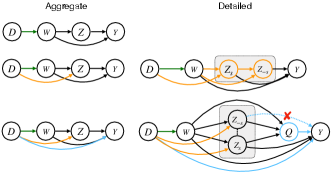
Here we introduce how the aggregate and detailed decompositions are defined for explaining the performance gap of a risk prediction algorithm for binary outcomes across source and target domains, denoted by and , respectively. Let the performance of be quantified in terms of a loss function , such as the 0-1 misclassification loss . Suppose variables can be partitioned into and , where . This partitioning allows for a factorization of the data distribution in the source domain and target domain into
| (1) |
(see Fig 2 top left). As such, we refer to as baseline variables and as conditional covariates. For the readmission example, may refer to demographics and to diagnosis codes. The total change in performance of can thus be written as where denotes the expectation over the distribution . A summary of notation used is provided in Table 2 of the Appendix.
Aggregate. At the aggregate level, the framework quantifies how replacing each factor in (1) from source to target contributes to the performance gap. We refer to such replacements as “aggregate shifts,” as the shift is not restricted to a particular subset of variables. This leads to the aggregate decomposition , where quantifies the impact of a shift in the baseline distribution (also known as marginal or covariate shifts (Quionero-Candela et al., 2009)), quantifies the impact of a shift in the conditional covariate distribution , and quantifies the impact of a shift in the outcome distribution (also known as concept shift). More concretely,
Prior works have proposed similar aggregate decompositions (Cai et al., 2023; Liu et al., 2023; Firpo et al., 2018).
Detailed. At the detailed level, the framework outputs Shapley-based variable attributions that describe how shifts with respect to each variable contribute to each term in the aggregate decomposition. Based on the VI values, an ML development team can better understand the underlying cause for a performance gap and brainstorm which mixture of operational interventions (e.g. changing data collection) and algorithmic interventions (e.g. retraining the model with respect to the variable(s)) would be most effective at closing the performance gap. For instance, a variable with high importance to the conditional covariate shift term can be due to differences in missingness rates, prevalence, or selection bias; and a variable with high importance to the conditional outcome shift term may indicate inherent differences in the conditional distribution (also known as effect modification), differences in measurement error or outcome definitions, or omission of variables predictive of the outcome. Note that the framework does not output a detailed decomposition of the baseline shift term , for reasons we discuss later.
We leverage the Shapley attribution framework for its axiomatic properties, which result in VI values with intuitive interpretations (Shapley, 1953; Charnes et al., 1988). Recall that for a real-valued value function defined for all subsets , the attribution to element is defined as the average gain in value due to the inclusion of to every possible subset, i.e.
So to define a detailed decomposition, the key question is how to define the value of a partial distribution shift only with respect to a variable subset ; henceforth we refer to such shifts as -partial shifts. It turns out that the answer is far from straightforward.
3.1 Value of partial distribution shifts
If the true causal graph is known, it would be straightforward to determine how the data distribution shifted with respect to a given variable subset : we would assign the value of subset as the change in overall performance due to shifts only in with respect to this graph. However, in the absence of more detailed causal knowledge, one can only hypothesize the form of partial distribution shifts. Some proposals define importance as the change in average performance due to hypothesized partial shifts (see e.g. Wu et al. (2021)), but it can lead to unintuitive behavior where a hypothesized distribution shift inconsistent with the true causal graph is attributed high importance. We illustrate such an example in a simulation in Section 5.
Instead, our proposal defines the importance of variable subset as the proportion of variation in performance changes across strata explained by its corresponding hypothesized -partial shift, denoted by . The definition generalizes the traditional measure in statistics, which quantifies how well do covariates explain variation in outcome rather than in performance changes. Prior works on variable importance have leveraged similar definitions (Williamson et al., 2021; Hines et al., 2023). For the conditional covariate decomposition, we define the value of as
| (2) |
where is the performance gap observed at in strata when is replaced with . (Note that we overload the notation where means source domain, means target domain, and means an -partial shift.) Setting , we denote the corresponding Shapley values by . Similarly, for the conditional outcome decomposition, we define the importance of as how well the hypothesized -partial outcome shift explains the variation in performance gaps across strata , i.e.
where Setting , we denote the corresponding Shapley values by . Because this framework defines importance in terms of variance explained, it does not provide a detailed decomposition of the baseline shift.
3.2 Candidate partial shifts
The previous section defines a general scoring scheme for quantifying the importance of any hypothesized -partial shift. In this work, we consider partial shifts of the following forms. We leave other forms of partial shifts to future work.
-partial conditional covariate shift: We hypothesize that is downstream of and define as , as illustrated in Fig 2 right top. A similar proposal was considered in Wu et al. (2021). For , note that .
In the readmission example, such a shift would hypothesize that certain diagnosis codes in are upstream of the others. For instance, one could reasonably hypothesize that diagnosis codes that describe family history of disease are upstream of the other diagnosis codes. Similarly, medical treatments/procedures are likely downstream of a patient’s baseline characteristics and comorbidities.
-partial conditional outcome shift: Shifting the conditional distribution of only with respect to a variable subset but not requires care. We cannot simply split into and , and define the distribution of solely as a function of and , because defining for some generally implies that even when .
Instead, we define an -partial outcome shift based on models commonly used in model recalibration/revision (Steyerberg, 2009; Platt, 1999), where the modified risk is a function of the risk in the source domain , , and . In particular, we define the shift as
| (3) | |||
By defining the shifted outcome distribution solely as a function of , and , it encompasses the special scenario where there is no conditional outcome shift and eliminates any direct effect from to . Note that may be non-zero when the risk in the target domain is a recalibration (i.e. temperature-scaling) of the risk in the source domain (Platt, 1999; Guo et al., 2017). For instance, there may be general environmental factors such that readmission risks in the target domain are uniformly lower.
In the readmission example, a partial outcome distribution shift may be due to, for instance, a hospital protocol where HF patients with given diagnoses (e.g. kidney failure) are scheduled for more frequent follow-ups than just having those diagnoses alone. Thus readmission risks in the HF population can be viewed as a fine-tuning of readmission risks in the general patient population with respect to .
4 Estimation and Inference
The key estimands in this hierarchical attribution framework are the aggregate terms , and and the Shapley-based detailed terms and for . We now provide nonparametric estimators for these quantities as well as statistical inference procedures for constructing CIs. Nearly all prior works for decomposing performance gaps have relied on plug-in estimators, which substitute in estimates of the conditional means (also known as outcome models) or density ratios (Sugiyama et al., 2007), which we collectively refer to as nuisance parameters. For instance, given ML estimators and for the conditional means and , respectively, the empirical mean of with respect to the target domain is a plug-in estimator for . However, because ML estimators typically converge to the true nuisance parameters at a rate slower than , plug-in estimators generally fail to be consistent at a rate of and cannot be used to construct CIs (Kennedy, 2022). Nevertheless, using tools from semiparametric inference theory (e.g. one-step correction and Neyman orthogonality), one can derive debiased ML estimators that facilitate statistical inference (Chernozhukov et al., 2018; Tsiatis, 2006). Here we derive debiased ML estimators for terms in the aggregate and detailed decompositions. The detailed conditional outcome decomposition is particularly interesting, as its unique structure is not amenable to standard techniques for debiasing ML estimators.
For ease of exposition, theoretical results are presented for split-sample estimators; nonetheless, the results readily extend to cross-fitted estimators under standard convergence criteria (Chernozhukov et al., 2018; Kennedy, 2022). Let denote independent and identically distributed (IID) observations from the source and target domains and , respectively. Let a fixed fraction of the data be partitioned towards “training” (Tr) and the remaining to “evaluation” (Ev); let be the number of observations in the evaluation partition. Let denote the expectation with respect to domain and denote the empirical average over observations in partition Ev from domain . All estimators are denoted using hat notation. Proofs, detailed theoretical results, and psuedocode are provided in the Appendix.
4.1 Aggregate decomposition
The aggregate decomposition terms can be formulated as an average treatment effect, a well-studied estimand in causal inference, where domain corresponds to treatment. As such, one can use augmented inverse probability weighting (AIPW) to define debiased ML estimators of the aggregate decomposition terms (e.g. (Kang & Schafer, 2007)). We review estimation and inference for these terms below.
Estimation. Using the training data, estimate outcome models and and density ratio models and . The debiased ML estimators for are
Inference. Assuming the estimators for the outcome and density ratio models converge at a fast enough rate, the AIPW estimators for the aggregate decomposition terms converge at the desired rate.
Theorem 4.1.
Suppose and are bounded; estimators , , , and are consistent; and
Then and are asymptotically linear estimators of their respective estimands.
4.2 Detailed decomposition
The Shapley-based detailed decomposition terms and for are an additive combination of the value functions that quantify the proportion of variability explained by -partial shifts. Below, we present novel estimators for values for -partial conditional outcome shifts, their theoretical properties, and computationally efficient estimation for their corresponding Shapley values. Due to space constraints, results pertaining to partial conditional covariate shifts are provided in Section B.1 of the Appendix.
4.2.1 Value of -partial outcome shifts
Standard recipes for deriving asymptotically linear, nonparametric efficient estimators rely on pathwise differentiability of the estimand and analyzing its efficient influence function (EIF) (Kennedy, 2022). However, is not pathwise differentiable because it is a function of (3), which conditions on the source risk equalling some value . Taking the pathwise derivative of requires taking a derivative of the indicator function , which generally does not exist. Given the difficulties in deriving an asymptotically normal estimator for , we propose estimating a close alternative that is pathwise differentiable.
The idea is to replace in (3) with its binned variant for some , which discretizes outputs from into disjoint bins. As long as is sufficiently high, the binned version of the estimand, denoted , is a close approximation to . (We use in the empirical analyses, which we believe to be sufficient in practice.) The benefit of this binned variant is that the derivative of the indicator function is zero almost everywhere as long as observations with source risks exactly equal to a bin edge is measure zero. More formally, we require the following:
Condition 4.2.
Let be the set of such that falls precisely on some bin edge but is not equal to zero or one. The set is measure zero.
Under this condition, is pathwise differentiable and, using one-step correction, we derive a debiased ML estimator that has the unique form of a V-statistic (this follows from the integration over “phantom” in (3)). We represent V-statistics using the operator , which takes the average over all pairs of observations from the evaluation partition with replacement, i.e. for some function . Calculation of this estimator and its theoretical properties are as follows.
Estimation. Using the training partition, estimate a density ratio model defined as and the -shifted outcome model . The estimator for is where is
| (4) | |||
where and is
| (5) | |||
Inference. This estimator is asymptotically linear assuming the nuisance estimators converge at a fast enough rate.
Theorem 4.3.
Suppose Condition 4.2 holds. For variable subset , suppose are bounded; ; estimator is consistent; estimators and converge at an rate, and
| (6) | ||||
Then the estimator is asymptotically normal centered at the estimand .
Convergence rate of can be achieved by ML estimators in a wide variety of conditions, and such assumptions are commonly used to construct debiased ML estimators. The additional requirement in (6) that converges at a rate is new, but fast or even super-fast convergence rates of binned risks is achievable under suitable margin conditions (Audibert & Tsybakov, 2007).
4.2.2 Shapley values
Calculating the exact Shapley value is computationally intractable as it involves an exponential number of terms. Nevertheless, Williamson & Feng (2020) showed that calculating the exact Shapley value for variable importance measures is not necessary when the importance measures are estimated with uncertainty. One can instead estimate the Shapley values by sampling variable subsets and inflate the corresponding CIs to reflect the additional uncertainty due to subset sampling. As long as the number of subsets scales linearly or super-linearly in , one can show that this additional uncertainty will not be larger than that due to estimation of subset values themselves. Here we follow the same procedure to estimate and construct CIs for the detailed decomposition Shapley values (see Algorithm 4).
5 Simulation
We now present simulations that verify the theoretical results by showing that the proposed procedure achieves the desired coverage rates (Sec 5.1) and illustrate how the proposed method provides more intuitive explanations of performance gaps (Sec 5.2). In all empirical analyses, performance of the ML algorithm is quantified in terms of 0-1 accuracy. Below, we briefly describe the simulation settings; full details are provided in Sec E in the Appendix.
5.1 Verifying theoretical properties
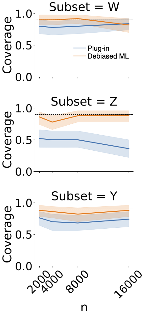
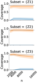
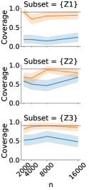
We first verify that the inference procedures for the decomposition terms have CIs with coverage close to their nominal rate. We check the coverage of the aggregate decomposition as well as the value of -partial conditional covariate and partial conditional outcome shifts for . are sampled from independent normal distributions with different means in source and target, while is simulated from logistic regression models with different coefficients. CIs for the debiased ML estimator converge to the nominal 90% coverage rate with increasing sample size, whereas those for the naïve plug-in estimator do not (Fig 3).
(a) Conditional covariate
(b) Conditional outcome
| Method | Acc-1 | Acc-2 | Acc-3 |
|---|---|---|---|
| ParametricChange | 0.78 | 0.80 | 0.81 |
| ParametricAcc | 0.75 | 0.80 | 0.80 |
| RandomForestAcc | 0.78 | 0.80 | 0.80 |
| OaxacaBlinder | 0.78 | 0.78 | 0.80 |
| Proposed | 0.80 | 0.80 | 0.81 |
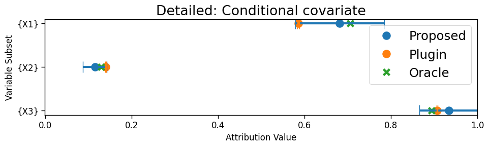
5.2 Comparing explanations
We now compare the proposed definitions for the detailed decomposition with existing methods. For the detailed conditional covariate decomposition, the comparators are:
-
•
MeanChange Tests for a difference in means for each variable. Defines importance as p-value.
-
•
Oaxaca-Blinder: Fits a linear model of the logit-transformed expected loss with respect to in the source domain. Defines importance of as its coefficient multiplied by the difference in the mean of (Blinder, 1973).
-
•
WuShift (Wu et al., 2021): Defines importance of subset as change in overall performance due to -partial conditional covariate shifts. Applies Shapley framework to obtain VIs.
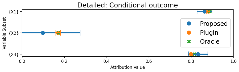
For the detailed decomposition of the performance gap due to shifts in the outcome, we compare against:
-
•
ParametricChange: Fits a logistic model for with interaction terms between domain and . Defines importance of as the coefficient of its interaction term.
-
•
ParametricAcc: Same as ParametricChange but models the 0-1 loss rather than .
-
•
RandomForestAcc: Compares VI of RFs trained on data from both domains with input features , , and to predict the 0-1 loss.
-
•
Oaxaca-Blinder: Fits linear models for the logit-transformed expected loss in each domain. Defines importance of as its mean in the target domain multiplied by the difference in its coefficients across domains.
Although the proposed method agrees on important features with these other methods in certain cases, there are important situations where the methods differ as highlighted below.
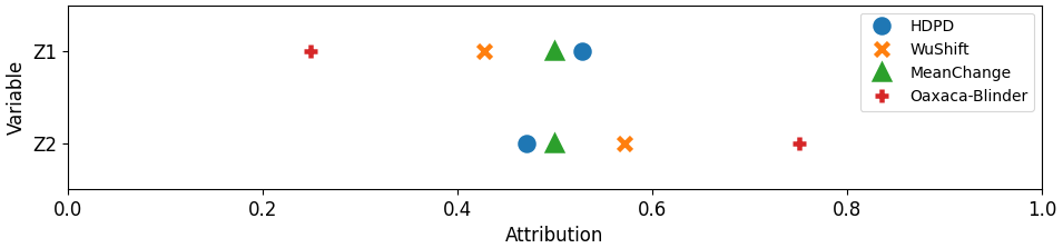
Conditional covariate. (Fig 4a) We simulate from a standard normal distribution, from a mixture of two Gaussians whose means depend on the value of (i.e. ), and from a logistic regression model depending on . We induce a shift from the source domain to the target domain by shifting only the distribution of , so that . Only the proposed estimator correctly recovers that is more important than , because this shift explains all the variation in performance gaps across strata . The other methods incorrectly assign higher importance to because they simply assess the performance change due to hypothesized -partial shifts but do not check if the hypothesized shifts are good explanations in the first place.
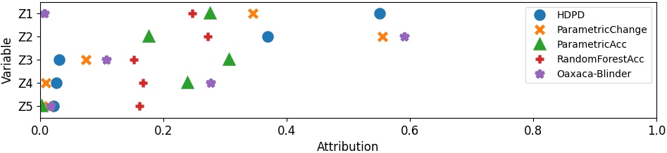
Conditional outcome. (Fig 4b) and are simulated from the same distribution in both domains. is generated from a logistic regression model with coefficients for as in the source and in the target. Interestingly, none of the methods have the same ranking of the features. ParametricChange identifies as having the largest shift on the logit scale, but this does not mean that it is the most important explanation for changes in the loss. According to our decomposition framework, is actually the most important for explaining changes in model performance due to outcome shifts. Oaxaca-Blinder and ParametricAcc have odd behavior—Oaxaca-Blinder assigns the lowest importance and ParametricAcc assigns the highest importance), because the models are misspecified. The VI from RandomForestAcc is also difficult to interpret because it measures which variables are good predictors of performance, not performance shift.
(a) Readmission risk prediction
(b) Insurance coverage prediction
Perhaps a more objective evaluation is to compare the utility of the different explanations. To this end, we define a targeted algorithmic modification as one where the source risk is revised with respect to a subset of features by fitting an ML algorithm with input features as , , and on the target domain. Comparing the performance of the targeted algorithmic modifications that take in the top features from each explanation method, we find that model revisions based on the proposed method achieve the highest performance for to .
6 Real-world data case studies
We now analyze two datasets with naturally-occurring shifts.
Hospital readmission. Using electronic health record data from a large safety-net hospital, we analyzed performance of a Gradient Boosted Tree (GBT) trained on the general patient population (source) to predict 30-day readmission risk but applied to patients diagnosed with HF (target). Features include 4 demographic variables () and 16 diagnosis codes (). Each domain supplied observations.
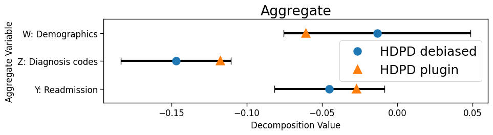
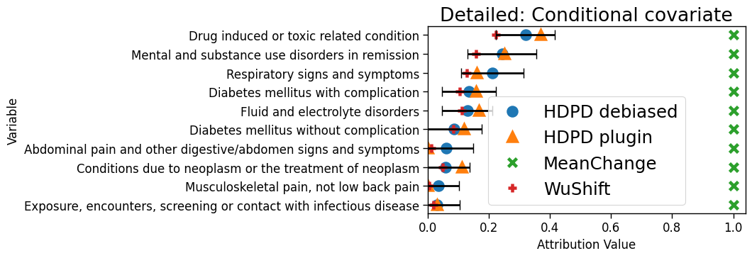
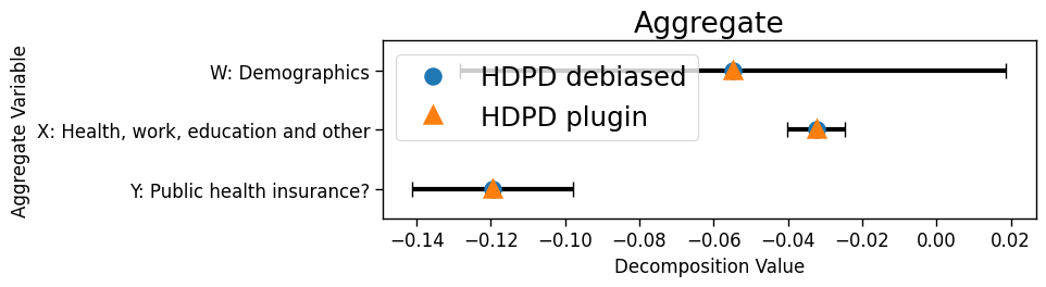
Model accuracy drops from 70% to 53%. From the aggregate decompositions (Fig 5a), we observe that the drop is mainly due to covariate shift. If one performed the standard check to see which variables significantly changed in their mean value (MeanChange), then one would find a significant shift in nearly every variable. Little support is offered to identify main drivers of the performance drop. In contrast, the detailed decomposition from the proposed framework estimates diagnoses “Drug-induced or toxic-related condition” and “mental and substance use disorder in remission” as having the highest estimated contributions to the conditional covariate shift, and most other variables having little to no contribution. Upon discussion with clinicians from this hospital, differences in the top two diagnoses may be explained by (i) substance use being a major cause of HF at this hospital, with over eighty percent of its HF patients reporting current or prior substance use, and (ii) substance use and mental health disorders often occurring simultaneously in this HF patient population. Based on these findings, closing the performance gap may require a mixture of both operational and algorithmic interventions. Finally, CIs from the debiased ML procedure provide valuable information on the uncertainty of the estimates and highlight, for instance, that more data is necessary to determine the true ordering between the top two features. In contrast, existing methods do not provide (asymptotically valid) CIs.
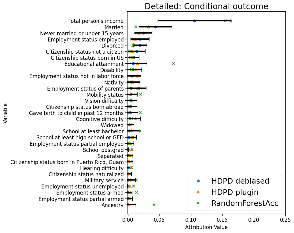
ACS Public Coverage. We analyze a neural network trained to predict whether a person has public health insurance using data from Nebraska in the American Community Survey (source, ), applied to data from Louisiana (target, ). Baseline variables include 3 demographics (sex, age, race), and covariates include 31 variables related to health conditions, employment, marital status, citizenship status, and education.
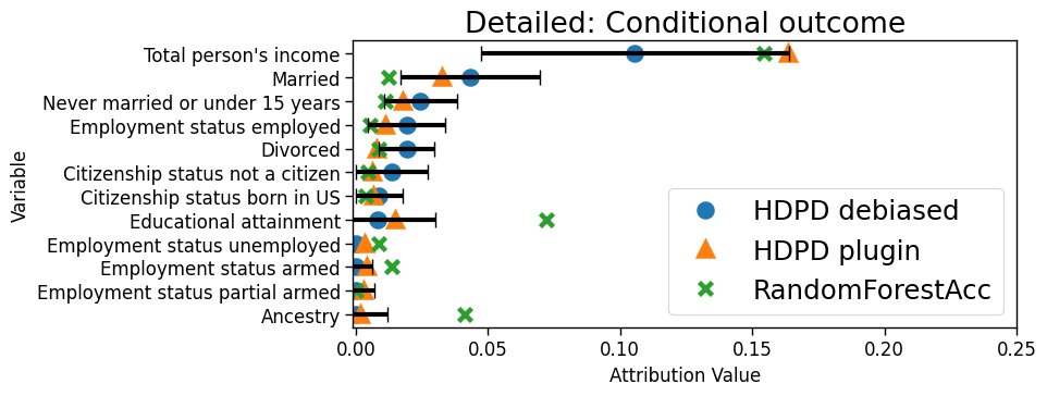
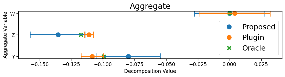
Model accuracy drops from 84% to 66% across the two states. The main driver is the shift in the outcome distribution per the aggregate decomposition (Fig 5b) and the most important contributor to the outcome shift is annual income, perhaps due to differences in cost of living across the two states. Income is significantly more important than all the other variables; the ranking between the remaining variables is unclear. In comparing the performance of targeted model revisions with respect to the top variables from each explanation method, we find that model revisions based on top variables identified by the proposed procedure lead to AUCs that are better or as good as those based on RandomForestAcc (Table 3 in the Appendix).
7 Discussion
ML algorithms regularly encounter distribution shifts in practice, leading to drops in performance. We present a novel framework that helps ML developers and deployment teams build a more nuanced understanding of the shifts. Compared to past work, the approach is nonparametric, does not require fine-grained knowledge of the causal relationship between variables, and quantifies the uncertainty of the estimates by constructing confidence intervals. We present case studies on real-world datasets to demonstrate the use of the framework for understanding and guiding interventions to reduce performance drops.
Extensions of this work include relaxing the assumption of overlapping support of covariates such as by restricting to the common support (Cai et al., 2023), allowing for decompositions of more complex measures of model performance such as AUC, and analyzing other factorizations of the data distribution (e.g. label or prior shifts (Kouw & Loog, 2019)). For unstructured data (e.g. image and text), the current framework can be applied to low-dimensional embeddings or by extracting interpretable concepts (Kim et al., 2018); more work is needed to extend this framework to directly analyze unstructured data. Finally, the focus of this work is to interpret performance gaps. Future work may extend ideas in this work to design optimal interventions for closing the performance gap.
Impact statement
This work presents a method for understanding failures of ML algorithms when they are deployed in settings or populations different from the ones in development datasets. Therefore, the work can be used to suggest ways of improving the algorithms or mitigating their harms. The method is generally applicable to tabular data settings for any classification algorithm, hence, it can potentially be applied across multiple domains where ML is used including medicine, finance, and online commerce.
Acknowledgments
We would like to thank Lucas Zier, Avni Kothari, Berkman Sahiner, Nicholas Petrick, Gene Pennello, Mi-Ok Kim, and Romain Pirracchio for their invaluable feedback on the work. This work was funded through a Patient-Centered Outcomes Research Institute® (PCORI®) Award (ME-2022C1-25619). The views presented in this work are solely the responsibility of the author(s) and do not necessarily represent the views of the PCORI®, its Board of Governors or Methodology Committee, and the Food and Drug Administration.
References
- Ali et al. (2022) Ali, A., Cauchois, M., and Duchi, J. C. The lifecycle of a statistical model: Model failure detection, identification, and refitting, 2022. URL https://arxiv.org/abs/2202.04166.
- Audibert & Tsybakov (2007) Audibert, J.-Y. and Tsybakov, A. B. Fast learning rates for plug-in classifiers. Ann. Stat., 35(2):608–633, April 2007.
- Blinder (1973) Blinder, A. S. Wage discrimination: Reduced form and structural estimates. The Journal of Human Resources, 8(4):436–455, 1973. ISSN 0022166X. URL http://www.jstor.org/stable/144855.
- Budhathoki et al. (2021) Budhathoki, K., Janzing, D., Bloebaum, P., and Ng, H. Why did the distribution change? In Banerjee, A. and Fukumizu, K. (eds.), Proceedings of The 24th International Conference on Artificial Intelligence and Statistics, volume 130 of Proceedings of Machine Learning Research, pp. 1666–1674. PMLR, 13–15 Apr 2021. URL https://proceedings.mlr.press/v130/budhathoki21a.html.
- Cai et al. (2023) Cai, T. T., Namkoong, H., and Yadlowsky, S. Diagnosing model performance under distribution shift. March 2023. URL http://arxiv.org/abs/2303.02011.
- Charnes et al. (1988) Charnes, A., Golany, B., Keane, M., and Rousseau, J. Extremal principle solutions of games in characteristic function form: Core, chebychev and shapley value generalizations. In Sengupta, J. K. and Kadekodi, G. K. (eds.), Econometrics of Planning and Efficiency, pp. 123–133. Springer Netherlands, Dordrecht, 1988.
- Chernozhukov et al. (2018) Chernozhukov, V., Chetverikov, D., Demirer, M., Duflo, E., Hansen, C., Newey, W., and Robins, J. Double/debiased machine learning for treatment and structural parameters. Econom. J., 21(1):C1–C68, February 2018.
- Cummings et al. (2023) Cummings, B. C., Blackmer, J. M., Motyka, J. R., Farzaneh, N., Cao, L., Bisco, E. L., Glassbrook, J. D., Roebuck, M. D., Gillies, C. E., Admon, A. J., et al. External validation and comparison of a general ward deterioration index between diversely different health systems. Critical Care Medicine, 51(6):775, 2023.
- d’Eon et al. (2022) d’Eon, G., d’Eon, J., Wright, J. R., and Leyton-Brown, K. The spotlight: A general method for discovering systematic errors in deep learning models. In 2022 ACM Conference on Fairness, Accountability, and Transparency, FAccT ’22, pp. 1962–1981, New York, NY, USA, 2022. Association for Computing Machinery. ISBN 9781450393522. doi: 10.1145/3531146.3533240. URL https://doi.org/10.1145/3531146.3533240.
- Dodd & Pepe (2003) Dodd, L. E. and Pepe, M. S. Semiparametric regression for the area under the receiver operating characteristic curve. J. Am. Stat. Assoc., 98(462):409–417, 2003.
- Eyuboglu et al. (2022) Eyuboglu, S., Varma, M., Saab, K. K., Delbrouck, J.-B., Lee-Messer, C., Dunnmon, J., Zou, J., and Re, C. Domino: Discovering systematic errors with cross-modal embeddings. In International Conference on Learning Representations, 2022. URL https://openreview.net/forum?id=FPCMqjI0jXN.
- Fairlie (2005) Fairlie, R. W. An extension of the blinder-oaxaca decomposition technique to logit and probit models. Journal of economic and social measurement, 30(4):305–316, 2005.
- Firpo et al. (2018) Firpo, S. P., Fortin, N. M., and Lemieux, T. Decomposing wage distributions using recentered influence function regressions. Econometrics, 6(2), 2018. ISSN 2225-1146. doi: 10.3390/econometrics6020028. URL https://www.mdpi.com/2225-1146/6/2/28.
- Fortin et al. (2011) Fortin, N., Lemieux, T., and Firpo, S. Chapter 1 - decomposition methods in economics. volume 4 of Handbook of Labor Economics, pp. 1–102. Elsevier, 2011. doi: https://doi.org/10.1016/S0169-7218(11)00407-2. URL https://www.sciencedirect.com/science/article/pii/S0169721811004072.
- Guo et al. (2017) Guo, C., Pleiss, G., Sun, Y., and Weinberger, K. Q. On calibration of modern neural networks. International Conference on Machine Learning, 70:1321–1330, 2017.
- Hines et al. (2022) Hines, O., Diaz-Ordaz, K., and Vansteelandt, S. Variable importance measures for heterogeneous causal effects. April 2022.
- Hines et al. (2023) Hines, O., Diaz-Ordaz, K., and Vansteelandt, S. Variable importance measures for heterogeneous causal effects, 2023.
- Jain et al. (2023) Jain, S., Lawrence, H., Moitra, A., and Madry, A. Distilling model failures as directions in latent space. In The Eleventh International Conference on Learning Representations, 2023. URL https://openreview.net/forum?id=99RpBVpLiX.
- Kang & Schafer (2007) Kang, J. D. Y. and Schafer, J. L. Demystifying Double Robustness: A Comparison of Alternative Strategies for Estimating a Population Mean from Incomplete Data. Statistical Science, 22(4):523 – 539, 2007. doi: 10.1214/07-STS227. URL https://doi.org/10.1214/07-STS227.
- Kennedy (2022) Kennedy, E. H. Semiparametric doubly robust targeted double machine learning: a review. March 2022.
- Kim et al. (2018) Kim, B., Wattenberg, M., Gilmer, J., Cai, C., Wexler, J., Viegas, F., and sayres, R. Interpretability beyond feature attribution: Quantitative testing with concept activation vectors (TCAV). In Dy, J. and Krause, A. (eds.), Proceedings of the 35th International Conference on Machine Learning, volume 80 of Proceedings of Machine Learning Research, pp. 2668–2677. PMLR, 10–15 Jul 2018. URL https://proceedings.mlr.press/v80/kim18d.html.
- Kirby et al. (2006) Kirby, J. B., Taliaferro, G., and Zuvekas, S. H. Explaining racial and ethnic disparities in health care. Medical Care, 44(5):I64–I72, 2006. ISSN 00257079. URL http://www.jstor.org/stable/3768359.
- Kouw & Loog (2019) Kouw, W. M. and Loog, M. An introduction to domain adaptation and transfer learning, 2019.
- Kulinski & Inouye (2023) Kulinski, S. and Inouye, D. I. Towards explaining distribution shifts. In Krause, A., Brunskill, E., Cho, K., Engelhardt, B., Sabato, S., and Scarlett, J. (eds.), Proceedings of the 40th International Conference on Machine Learning, volume 202 of Proceedings of Machine Learning Research, pp. 17931–17952. PMLR, 23–29 Jul 2023. URL https://proceedings.mlr.press/v202/kulinski23a.html.
- Kulinski et al. (2020) Kulinski, S., Bagchi, S., and Inouye, D. I. Feature shift detection: Localizing which features have shifted via conditional distribution tests. In Larochelle, H., Ranzato, M., Hadsell, R., Balcan, M., and Lin, H. (eds.), Advances in Neural Information Processing Systems, volume 33, pp. 19523–19533. Curran Associates, Inc., 2020. URL https://proceedings.neurips.cc/paper/2020/file/e2d52448d36918c575fa79d88647ba66-Paper.pdf.
- Liu et al. (2023) Liu, J., Wang, T., Cui, P., and Namkoong, H. On the need for a language describing distribution shifts: Illustrations on tabular datasets. July 2023.
- Oaxaca (1973) Oaxaca, R. Male-female wage differentials in urban labor markets. International Economic Review, 14(3):693–709, 1973. ISSN 00206598, 14682354. URL http://www.jstor.org/stable/2525981.
- Pedregosa et al. (2011) Pedregosa, F., Varoquaux, G., Gramfort, A., Michel, V., Thirion, B., Grisel, O., Blondel, M., Prettenhofer, P., Weiss, R., Dubourg, V., Vanderplas, J., Passos, A., Cournapeau, D., Brucher, M., Perrot, M., and Duchesnay, E. Scikit-learn: Machine learning in Python. Journal of Machine Learning Research, 12:2825–2830, 2011.
- Platt (1999) Platt, J. Probabilistic outputs for support vector machines and comparisons to regularized likelihood methods. Advances in large margin classifiers, 10(3):61–74, 1999.
- Plumb et al. (2023) Plumb, G., Johnson, N., Cabrera, A., and Talwalkar, A. Towards a more rigorous science of blindspot discovery in image classification models. Transactions on Machine Learning Research, 2023. ISSN 2835-8856. URL https://openreview.net/forum?id=MaDvbLaBiF. Expert Certification.
- Qiu et al. (2023) Qiu, H., Tchetgen, E. T., and Dobriban, E. Efficient and multiply robust risk estimation under general forms of dataset shift. June 2023.
- Quionero-Candela et al. (2009) Quionero-Candela, J., Sugiyama, M., Schwaighofer, A., and Lawrence, N. D. Dataset shift in machine learning. The MIT Press, 2009.
- Rabanser et al. (2019) Rabanser, S., Günnemann, S., and Lipton, Z. Failing loudly: An empirical study of methods for detecting dataset shift. In Wallach, H., Larochelle, H., Beygelzimer, A., d'Alché-Buc, F., Fox, E., and Garnett, R. (eds.), Advances in Neural Information Processing Systems, volume 32. Curran Associates, Inc., 2019. URL https://proceedings.neurips.cc/paper/2019/file/846c260d715e5b854ffad5f70a516c88-Paper.pdf.
- Shapley (1953) Shapley, L. S. 17. a value for n-person games. In Kuhn, H. W. and Tucker, A. W. (eds.), Contributions to the Theory of Games (AM-28), Volume II, pp. 307–318. Princeton University Press, Princeton, December 1953.
- Steyerberg (2009) Steyerberg, E. W. Clinical Prediction Models: A Practical Approach to Development, Validation, and Updating. Springer, New York, NY, 2009.
- Sugiyama et al. (2007) Sugiyama, M., Nakajima, S., Kashima, H., Buenau, P., and Kawanabe, M. Direct importance estimation with model selection and its application to covariate shift adaptation. Adv. Neural Inf. Process. Syst., 2007.
- Tsiatis (2006) Tsiatis, A. A. Semiparametric Theory and Missing Data. Springer New York, 2006.
- van der Vaart (1998) van der Vaart, A. W. Asymptotic Statistics. Cambridge University Press, October 1998.
- Williamson & Feng (2020) Williamson, B. D. and Feng, J. Efficient nonparametric statistical inference on population feature importance using shapley values. International Conference on Machine Learning, 2020. URL https://proceedings.icml.cc/static/paper_files/icml/2020/3042-Paper.pdf.
- Williamson et al. (2021) Williamson, B. D., Gilbert, P. B., Carone, M., and Simon, N. Nonparametric variable importance assessment using machine learning techniques. Biometrics, 77(1):9–22, 2021. doi: https://doi.org/10.1111/biom.13392. URL https://onlinelibrary.wiley.com/doi/abs/10.1111/biom.13392.
- Wu et al. (2021) Wu, E., Wu, K., and Zou, J. Explaining medical AI performance disparities across sites with confounder shapley value analysis. November 2021. URL http://arxiv.org/abs/2111.08168.
- Yun (2004) Yun, M.-S. Decomposing differences in the first moment. Economics Letters, 82(2):275–280, 2004. ISSN 0165-1765. doi: https://doi.org/10.1016/j.econlet.2003.09.008. URL https://www.sciencedirect.com/science/article/pii/S0165176503002866.
- Zhang et al. (2023) Zhang, H., Singh, H., Ghassemi, M., and Joshi, S. ”Why did the model fail?”: Attributing model performance changes to distribution shifts. In Krause, A., Brunskill, E., Cho, K., Engelhardt, B., Sabato, S., and Scarlett, J. (eds.), Proceedings of the 40th International Conference on Machine Learning, volume 202 of Proceedings of Machine Learning Research, pp. 41550–41578. PMLR, 23–29 Jul 2023. URL https://proceedings.mlr.press/v202/zhang23ai.html.
Appendix A Contents of the Appendix
-
•
Table 1 summarizes the comparison with prior work.
-
•
Table 2 collects all the notation used for reference.
- •
-
•
Section B describes the estimation and inference for detailed decomposition of conditional covariate shift.
-
•
Section C provides the derivations of the results.
- •
-
•
Section F provides additional details on the two real world datasets and results.
| Papers | Aggregate decomp. | Detailed decomp. | Does not require knowing causal DAG | Confidence intervals | Nonparametric | |
| Cond. covariate | Cond. outcome | |||||
| Zhang et al. (2023) | ||||||
| Cai et al. (2023) | ||||||
| Wu et al. (2021) | ||||||
| Liu et al. (2023) | ||||||
| Dodd & Pepe (2003) | ||||||
| Oaxaca (1973), Blinder (1973) | ||||||
| HDPD (this paper) | ||||||
| Symbol | Meaning |
|---|---|
| Variables: Baseline, Conditional covariates, Outcome | |
| Prediction model being analyzed | |
| or | Loss function e.g. 0-1 loss |
| and | Indicators for source and target domain |
| Probability density (or mass) function for the two domains | |
| Expectation over the distribution | |
| Source domain risk at , i.e. | |
| Tr and Ev | Training dataset used to fit models and evaluation dataset used to compute decompositions |
| and | Shapley values for variable in the detailed decomposition of conditional covariate and outcome shifts |
| and | Value of a subset for -partial conditional covariate shift and -partial outcome shift |
| and | Numerator and denominator of the ratio defined in the value of a subset |
| Models | Outcome models for the conditional expectation of the loss across different settings |
| Models | Density ratio models for feature densities across datasets |
| Notation for expectation | |
| and | sample average over source and target data in the evaluation dataset |
| Influence function defined in the linear approximation of an estimand, see e.g. (11) |
Input: Source and target data for , loss function .
Output: Performance change due to baseline, conditional covariate, and conditional outcome shifts .
Split source and target data into training Tr and evaluation Ev partitions. Let be the total number of data points in the Ev partition.
Estimate using fitted nuisance parameters on the Ev partitions following the equations in Section 4.1.
Compute -level confidence intervals as for , where is the inverse CDF of the standard normal distribution.
return and confidence intervals
Input: Training Tr and evaluation Ev partitions of source and target data, subset of variables .
Output: Value for -partial conditional outcome shift for subset .
Estimate variance of influence function as defined in (63).
Compute -level confidence interval as .
return and confidence interval
Input: Training Tr and evaluation Ev partitions of source and target data, subset of variables .
Output: Value for -partial conditional covariate shift for subset .
Estimate by using (10) on the Ev partition.
Estimate variance of influence function as defined in (30).
Compute -level confidence interval as .
return and confidence interval
Input: Source and target data for , loss function , .
Output: Detailed decomposition for conditional outcome or covariate shift, or .
Split source and target data into training Tr and evaluation Ev partitions. Let be the total number of data points in the Ev partition.
Subsample subsets from with respect to Shapley weights, including and , denoted .
Estimate ValueConditionalOutcome(s) and ValueConditionalCovariate(s) for .
Get estimated Shapley values and by solving constrained linear regression problems in (7) in Williamson & Feng (2020) with value functions and , respectively.
Compute confidence intervals based on the influence functions defined in Theorem 1 in Williamson & Feng (2020).
return Shapley values and and confidence intervals
Appendix B Estimation and Inference
B.1 Value of -partial conditional covariate shifts
Estimation. Using the training partition, estimate the density ratio and the outcome models
| (7) | ||||
| (8) | ||||
| (9) |
in addition to the other nuisance models previously mentioned. We propose the estimator , where
| (10) | ||||
and .
Inference. The estimator is asymptotically normal as long as the outcome and density ratio models are estimated at a fast enough rate defined formally as follows.
Condition B.1.
For variable subset , suppose the following holds
-
•
is bounded
-
•
-
•
-
•
-
•
-
•
(Positivity) and almost everywhere, such that the density ratios and are well-defined and between .
Theorem B.2.
For variable subset , suppose and Condition B.1 hold. Then the estimator is asymptotically normal.
Appendix C Proofs
Notation. For all proofs, we will write to mean (and likewise for the empirical version) for notational simplicity.
Overview of derivation strategy. We first present the general strategy for proving asymptotic normality of the estimators for the decompositions. Details on nonparametric debiased estimation can be found in texts such as Tsiatis (2006) and Kennedy (2022).
Let be a pathwise differentiable quantity that is a function of the true regular (differentiable in quadratic mean) probability distribution over random variable . For instance, in the case of mean is defined as . Let denote an arbitrary regular estimator of , such as the maximum likelihood estimator. The plug-in estimator is then defined as .
The von-Mises expansion of the functional (which linearizes in analogy to the first-order Taylor expansion), given it is pathwise differentiable, gives
| (11) |
Here, the function is called an influence function (or a functional gradient of at ). is a second-order remainder term. The one-step corrected estimators we consider have the form of where denotes a sample average. Following the expansion above, the one-step corrected estimator can be analyzed as follows,
Our goal will be to analyze each of the three terms and to show that they are asymptotically negligible at -rate, such that the one-step corrected estimator satisfies
where we used the property of influence functions that they have zero mean. Thus the one-step corrected estimator is asymptotically normal with mean and variance , which allows for the construction of CIs. In the following proofs, we present the influence functions without derivations; see Kennedy (2022) and Hines et al. (2022) for strategies for deriving influence functions.
C.1 Aggregate decompositions
Let the nuisance parameters in the one-step estimators be denoted by respectively. Denote the estimated nuisances by . The canonical gradients for the three estimands are
| (12) | ||||
| (13) | ||||
| (14) |
Theorem C.1 (Theorem 4.1).
Under conditions outlined in Theorem 4.1, the one-step corrected estimators for the aggregate decomposition terms, baseline, conditional covariate, and conditional outcome , , and , are asymptotically linear, i.e.
| (15) |
Proof.
The estimands have similarities to the standard average treatment effect (ATE) in the causal inference literature (see (Kennedy, 2022, Example 2). Hence, the estimators and their asymptotic properties directly follow. For treatment , outcome , and confounders , the mean outcome under among the population with is identified as
| (16) |
and its one-step corrected estimator can be derived from the canonical gradient of , which takes the following form after plugging in the estimates of the nuisance models:
satisfies
where and as long as the following conditions hold:
-
•
almost everywhere such that the density ratios are well-defined and bounded,
-
•
.
We establish the estimators and their influence functions by showing that they can all be viewed as mean outcomes of the form (16).
Baseline term . The first term is a mean outcome with respect to , which is the same as that in (16) but with as the outcome, as the confounder, and as the (flipped) treatment. The second term is a simple average over population whose influence function is the itself.
Conditional covariate term . First term is the mean outcome with respect to , where the chief difference is is the confounder. Second term is also a mean outcome, as discussed above.
Conditional outcome term . First term is a simple average over the population. ∎
C.2 Value of -partial conditional covariate shifts
Let nuisance parameters in the one-step estimator be denoted and the set of estimated nuisances by . The canonical gradient of is
| (17) |
Lemma C.2.
Under Condition B.1, satisfies
| (18) | ||||
| (19) |
Proof.
Consider the following decomposition
| (20) | ||||
| (21) | ||||
| (22) |
We note that (21) converges to a normal distribution per CLT assuming the variance of is finite. The empirical process term (21) is asymptotically negligible, as the nuisance parameters are estimated using a separate training data split from the evaluation data and (Kennedy, 2022, Lemma 1) states that
as long as estimators for all nuisance parameters are consistent. We now establish that the remainder term (22) is also asymptotically negligible. Integrating with respect to , we have that
| (23) | ||||
| (24) | ||||
| (25) | ||||
| (26) |
From convergence conditions in Condition B.1, this simplifies to
| (27) | ||||
| (28) | ||||
| (29) |
Given the true density ratios, we can further simplify the expectations over weighted by the density ratios in the expression above to expectations over . By definition of in (7) and in (9) and the definition of and in Section 4.1, (22) simplifies to
which is as long as the convergence conditions in Condition B.1 hold.
As the denominator is equal to the numerator , it follows that the one-step estimator for the denominator is asymptotically linear with influence function . ∎
C.3 Value of -partial conditional outcome shifts
Let the nuisance parameters in be denoted and its estimate as .
We represent the one-step corrected estimator for as the V-statistic
| (32) | ||||
| (33) | ||||
| (34) | ||||
| (35) |
In more detail, the conditions in Theorem 4.3 are as follows.
Condition C.3.
For variable subset , suppose the following hold
-
•
is bounded
-
•
is consistent
-
•
-
•
-
•
-
•
-
•
.
Lemma C.4.
Assuming Condition C.3 holds, is an asymptotically linear estimator for , i.e.
| (36) |
with influence function
| (37) |
Proof.
Defining the symmetrized version of in (35) as , we rewrite the estimator as
Consider the decomposition
| (38) | ||||
| (39) | ||||
| (40) | ||||
| (41) |
We analyze each term in turn.
Term (38): Suppose . Via a straightforward extension of the proof in Theorem 12.3 in van der Vaart (1998), one can show that
Then by Theorem 11.2 in van der Vaart (1998) and Slutsky’s lemma, we have
Term (39): We perform sample splitting to estimate the nuisance parameters and calculate the estimator for . Then by Lemma 1 in Kennedy (2022), we have that
as long as the estimators for the nuisance parameters are consistent.
Term (40): This term follows an asymptotic normal distribution per CLT.
Condition C.5 (Convergence conditions for ).
Suppose the following holds
-
•
-
•
-
•
is bounded
-
•
(Positivity) almost everywhere, such that the density ratios are well-defined and bounded.
Let the nuisance parameters in the one-step estimator be denoted by and the set of estimated nuisances by .
Lemma C.6.
Assuming Condition C.5 holds, then is an asymptotically linear estimator for , i.e.
with influence function
| (46) | ||||
| (47) | ||||
| (48) | ||||
| (49) |
Proof.
Consider the following decomposition of bias in the one-step corrected estimate
| (50) | ||||
| (51) | ||||
| (52) |
We observe that (50) converges to a normal distribution per CLT assuming that the variance of is finite. The empirical process term (51) is asymptotically negligible since the nuisance parameters are evaluated on an separate evaluation data split from the training data used for estimation. In addition assuming that the estimators for the nuisance parameters are consistent, Kennedy (2022, Lemma 1) states that
Appendix D Implementation details
Here we describe how the nuisance parameters can be estimated in each of the decompositions. In general, density ratio models can be estimated via a standard reduction to a classification problem where a probabilistic classifier is trained to discriminate between source and target domains (Sugiyama et al., 2007).
Note on computation time. Shapley value computation can be parallelized over the subsets. For high-dimensional tabular data, grouping together variables can further reduce computation time (and increase interpretability).
D.1 Aggregate decompositions
Density ratio models. Using direct importance estimation (Sugiyama et al., 2007), density ratio models and can be estimated by fitting classifiers on the combined source and target data to predict or from features and , respectively.
Outcome models. The outcome models and can be fit in a number of ways. One option is to estimate the conditional distribution of the outcome (i.e. or ) using binary classifiers, from which one can obtain an estimate of the conditional expectation of the loss. Alternatively, one can estimate the conditional expectations of the loss directly by fitting regression models.
D.2 Detailed decomposition for -partial outcome shift
Density ratio models. The density ratio in (4) can be estimated as follows. Create a second (“phantom”) dataset of the target domain in which is independent of by permuting the original in the target domain. Compute for all observations in the original dataset and the permuted dataset. Concatenate the original dataset from the target domain with the permuted dataset. Train a classifier to predict if an observation is from the original versus the permuted dataset.
Outcome models. The outcome models and can be similarly fit by estimating the conditional distribution and on the target domain, and then taking expectation of the loss.
Computing U-statistics. Calculating the double average in the estimator requires evaluating all pairs of data points in target domain. This can be computationally expensive, so a good approximation is to subsample the inner average. We take 2000 subsamples. We did not see large changes in the bias of the estimates compared to calculating the exact U-statistics.
D.3 Detailed decomposition for -partial conditional outcome shift
Density ratio models. The ratio can be similarly fit using direct importance estimation.
Outcome models. We require the following models.
For all models, we use cross-validation to select among model types and hyperparameters. Model selection is important so that the convergence rate conditions for the asymptotic normality results are met.
Appendix E Simulation details
Data generation: We generate synthetic data under two settings. For the coverage checks in Section 5.1, all features are sampled independently from a multivariate normal distribution. The mean of the in the source and target domains are and , respectively. The outcome in the source and target domains are simulated from a logistic regression model with coefficients and .
In the second setting for baseline comparisons in Figure 4b, each feature in and is sampled independently from the rest from a uniform distribution over . The binary outcome is sampled from a logistic regression model with coefficients in source and in target.
Sample-splitting: We fit all models on 80% of the data points from both source and target datasets which is the Tr partition, and keep the remaining 20% for computing the estimators which is the Ev partition.
Model types: We use scikit-learn implementations for all models (Pedregosa et al., 2011). We use 3-fold cross validation to select models. For density models, we fit random forest classifiers and logistic regression models with polynomial features of degree 3. Depending on whether the target outcome in outcome models is binary or real-valued, we fit random forest classifiers or regressors, and logistic regression or linear regression models with ridge penalty. Specific hyperparameter ranges for the grid search will be provided in the code, to be made publicly available.
Computing time and resources: Computation for the VI estimates can be quite fast, as Shapley value computation can be parallelized over the subsets and the number of unique variable subsets sampled in the Shapley value approximation is often quite small. For instance, for the ACS Public Coverage case study with 34 features, the unique subsets is even when the number of sampled subsets is , and it takes around 160 seconds to estimate the value of a single variable subset. All experiments are run on a 2.60 GHz processor with 8 CPU cores.
Appendix F Data analysis details
Synthetic. We describe accuracy of the ML algorithm after it is retrained with the top features and predictions from the original model.
Hospital readmission. Using data from the electronic health records of a large safety-net hospital in the US, we analyzed the transferability of performance measures of a Gradient Boosted Tree (GBT) trained to predict 30-day readmission risk for the general patient population (source) but applied to patients diagnosed with heart failure (target). Each of the source and target datasets have 3750 observations for analyzing the performance gap. The GBT is trained on a held-out sample of 18,873 points from the general population. Features include 4 demographic variables () and 16 diagnosis codes (). While training, we reweigh samples by class weights to address class imbalance.
ACS Public Coverage. We extract data from the American Community Survey (ACS) to predict whether a person has public health insurance. The data only contains persons of age less than 65 and having an income of less than $30,000. We analyze a neural network (MLP) trained on data from Nebraska (source) to data from Louisiana (target) given 3000 and 6000 observations from the source and target domains, respectively. Another 3300 from source for training the model. Figure 7 shows the detailed decomposition of conditional outcome shift for the dataset.
| k | Diff AUC-k | Lower CI | Upper CI |
|---|---|---|---|
| 1 | 0.000 | 0.000 | 0.000 |
| 2 | 0.006 | 0.001 | 0.010 |
| 3 | -0.002 | -0.007 | 0.002 |
| 4 | 0.004 | -0.002 | 0.008 |
| 5 | -0.001 | -0.006 | 0.003 |
| 6 | -0.002 | -0.008 | 0.003 |
| 7 | 0.007 | 0.002 | 0.011 |
| 8 | 0.006 | 0.001 | 0.010 |