A high-order study of the quantum critical behavior of a frustrated spin-$\frac{1}{2}$ antiferromagnet on a stacked honeycomb bilayer

Quantum spin-lattice models, in which various types of interactions between pairs of spins compete to form different types of order in the system, provide a rich arena in which to study a wide variety of quantum phase transitions (QPTs) Sachdev (2011, 2008). Such competition can occur either with or without magnetic frustration between the interaction bonds. In the latter case the bonds are typically spatially anisotropic. Simple examples of such systems comprise models containing nearest-neighbor (NN) exchange interactions between spins $\mathbf{s}_{i}$ on lattice sites $i$ of the Heisenberg type, $J_{ij}\,\mathbf{s}_{i}\cdot\mathbf{s}_{j}$, all with bond strength $J_{ij}>0$, and thus all acting to promote antiferromagnetic (AFM) long-range order (LRO), but where the strengths $J_{ij}$ are not all equal. The so-called coupled-dimer magnets comprise a particularly simple, yet important and nontrivial, class of this type.

Dimerized quantum Heisenberg antiferromagnets (HAFMs) are obtained by placing quantum spins, with spin quantum number $s$, on a regular $d$-dimensional lattice with an even number of spins per unit cell. Each unit cell is divided into non-overlapping pairs of spins (dimers). In the limit where the intradimer exchange constant $J_{ij}$ are much stronger than all of the corresponding interdimer constants, the zero-temperature ($T=0$) ground-state (GS) phase of the system is a simple paramagnetic product of non-magnetic spin singlets, which preserves the full spin-rotational invariance. This state has a nonzero energy gap to the lowest-lying spin triplet excitation, formed by breaking one of the spin-singlet dimers. As the interdimer exchange interactions are turned on these triplet excitations acquire mobility on the lattice, resulting in the appearance of a spin-1 bosonic quasiparticle, viz., the triplon Schmidt and Uhrig (2003). In principle, of course, such bosons may undergo Bose-Einstein condensation (BEC) under suitable conditions and become superfluid. Indeed, such a superfluid state has been observed experimentally in the magnetic insulator TlCuCl₃ Nikuni et al. (2000); Cavadini et al. (2001); Rüegg et al. (2003); Oosawa et al. (2003), which is a physical realization of such a coupled-dimer magnet, in which pairs of Cu²⁺ ions are antiferromagnetically coupled to form a crystalline network of dimers in a specific pattern. The BEC is induced by placing the compound in an external magnetic field, which thereby Zeeman splits the otherwise degenerate three magnetic triplet sub-states. At some critical field strength the lowest-lying triplet state intersects the GS dimer singlet, and BEC into this triplon sub-state occurs, with the consequent appearance of the magnetic LRO corresponding to the off-diagonal LRO that characterizes BEC in the boson-mapped equivalent system. The whole area of BEC in magnetic insulators Giamarchi et al. (2008) has become one of considerable activity in recent years, at both the theoretical and experimental levels. The applied magnetic field here thus acts as a chemical potential that promotes dimer spin-singlets (leaving a hole) to spin-triplets (creating a triplon).

In principle, another way to induce magnetic LRO in a coupled-dimer magnet, without the application of an external magnetic field, is to increase the relative strength of the interdimer couplings $J_{ij}$ with respect to their intradimer counterparts. For example, for all two-dimensional (2D) bipartite lattices and with all couplings $J_{ij}$ between NN pairs only, when all $J_{ij}$ are equal the system will have Néel AFM magnetic LRO. Thus, if we consider the class of so-called $J$–$J^{\prime}$ models on bipartite lattices, in which the intradimer NN bonds all have the same strength $J^{\prime}>0$ and the interdimer NN bonds all have the same strength $J>0$, there will clearly be same critical value of the relative strength parameter, $(J^{\prime}/J)_{c}>1$, that marks a QPT between a Néel-ordered AFM GS phase and a dimerized paramagnetic GS phase. Experimentally, both in principle and sometimes in practice, such QPTs can be driven by the application of pressure to the system.

On the 2D square lattice with NN interactions only, $J$–$J^{\prime}$ models with specific arrangements of the $J^{\prime}$ bonds that have been studied include the columnar-dimer, staggered-dimer, and herringbone-dimer models (and see, e.g., Ref. Fritz et al. (2011)). The first two, each with two sites per unit cell, both have the dimer $J^{\prime}$ bonds parallel (say, along the row direction of the square lattice). Whereas in the columnar arrangement each basic square plaquette contains either two or no dimer $J^{\prime}$ bonds, in the staggered arrangement each basic square plaquette contains a single $J^{\prime}$ dimer bond. Finally, the herringbone-dimer model contains four sites per unit cell with two isolated (non-touching) dimer $J^{\prime}$ bonds perpendicular to one another. Each basic square plaquette also contains a single $J^{\prime}$ dimer bond. Interestingly, in the limit $J^{\prime}/J\rightarrow 0$, both the staggered-dimer and herringbone-dimer models become equivalent to the HAFM on a hexagonal lattice. Thus, both of these models interpolate between HAFMs on the hexagonal and square 2D lattices for values of $J^{\prime}/J$ in the range $0\leq J^{\prime}/J\leq 1$.

So far we have considered coupled-dimer magnets that include competition between bonds without frustration. The inclusion of extra bonds can now lead us into the realm of magnetic frustration, which adds further to the complexity and inherent interest of these models. For example, increasing frustration can have the effect of enhancing the repulsive interactions between triplons. In turn this can then eventually lead to the stablization of incompressible phases that break the translational symmetry of the lattice. If such GS phases of the system are placed in an external magnetic field, the itinerant triplons become localized in a crystalline phase.

Such phases have been observed experimentally in the spin-gap material SrCu₂(BO₃)₂ Kageyama et al. (1999); Kodama et al. (2002); Miyahara and Ueda (2003), which is well modeled Miyahara and Ueda (1999) by the 2D Shastry-Sutherland model Sriram Shastry and Sutherland (1981). This is a spin-$\frac{1}{2}$ coupled-dimer model on a square lattice, with four sites per unit cell, in which all NN pairs have an AFM Heisenberg bond of equal strength $J$, and the equivalent AFM dimer bonds, all of equal strength $J^{\prime}$, join non-overlapping diagonal next-nearest-neighbor (NNN) pairs in an orthogonal pattern. The unit cell thus contains two orthogonal dimers arranged across NNN diagonal pairs. Clearly, in the limit $J\rightarrow 0$ the model reduces to a Hamiltonian of decoupled dimers. This dimerized state then remains the exact GS phase Sriram Shastry and Sutherland (1981) for all values of $(J^{\prime}/J)$ above a certain critical value $(J^{\prime}/J)_{c}$. In the opposite limit, when $J^{\prime}\rightarrow 0$, the model reduces to the pure spin-$\frac{1}{2}$ HAFM (i.e., with NN interactions only) on the square lattice, which has Néel AFM magnetic LRO. In between, when $J^{\prime}=J$, the model reduces to the pure spin-$\frac{1}{2}$ HAFM on another of the 11 2D Archimedean lattices, the GS phase of which is also known to have Néel order Farnell et al. (2014), which implies $(J^{\prime}/J)_{c}>1$. Various theoretical studies (see, e.g., Refs. Koga and Kawakami (2000); Corboz and Mila (2013)) yield $(J^{\prime}/J)_{c}\approx 1.48$. In the Shastry-Sutherland material SrCu₂(BO₃)₂, for which $(J^{\prime}/J)\approx 1.6$, the triplon crystalline phases show up as a series of magnetization plateaux at unconventional filling fractions Kodama et al. (2002); Miyahara and Ueda (2003) that are stabilized by complex many-body interactions among the triplons Fritz et al. (2011); Miyahara and Ueda (2003); Abendschein and Capponi (2008); Dorier et al. (2008). Indeed, the magnetization plateaux in SrCu₂(BO₃)₂ at low magnetization are now quite well understood in terms of triplon bound states Corboz and Mila (2014); Foltin et al. (2014).

Since both BEC and crystalline phases of triplons can occur in frustrated coupled dimer magnets subjected to an external magnetic field, it is natural to wonder whether such systems might also exhibit the magnetic equivalent of supersolidity, in which a stable GS phase exhibits simultaneously both the diagonal LRO typical of a solid and the off-diagonal LRO typical of a superfluid. Such field-induced spin supersolidity has particularly been investigated for various frustrated spin-$\frac{1}{2}$ models on a square-lattice bilayer Giamarchi et al. (2008); Laflorencie and Mila (2007); Schmidt et al. (2008); Picon et al. (2008); Chen et al. (2010); Albuquerque et al. (2011); Murakami et al. (2013).

Such bilayer models provide other examples of coupled-dimer magnets. The simplest such bilayer models comprise two layers stacked directly on top of one another and with only NN bonds, where the intralayer bonds all have equal strength $J_{1}$ and the interlayer (dimer) bonds all have equal strength $J_{1}^{\perp}$. Such models on the square lattice, where the bonds compete without frustration, have been studied fairly extensively Sandvik et al. (1995); Chubukov and Morr (1995); Millis and Monien (1996); Wang et al. (2006); Ganesh et al. (2011). As the ratio $J_{1}^{\perp}/J_{1}$ is increased beyond a critical value $(J_{1}^{\perp}/J_{1})_{c}$ a QPT occurs from a Néel-ordered GS phase to a paramagnetic GS phase that is approximately the product of interlayer dimer valence bonds between NN pairs coupled by $J_{1}^{\perp}$ bonds. As we have already noted above, the $T=0$ GS phase diagram becomes appreciably richer in the additional presence of frustrating bonds of either the intralayer or interlayer type. Such frustrated square-lattice bilayer models have been much studied in recent years, using a variety of theoretical techniques, both in the absence Lin and Shen (2000); Alet et al. (2016) and presence Giamarchi et al. (2008); Chen et al. (2010); Albuquerque et al. (2011); Murakami et al. (2013); Richter et al. (2006); Derzhko et al. (2010) of an external magnetic field.

In the last several years attention has also been paid to analogous honeycomb-lattice bilayer models, both in the staggered Bernal AB stacking (see, e.g., Ref. Lee and Sachdev (2014)) relevant to bilayer graphene and in the $AA$ stacking (see, e.g., Refs. Ganesh et al. (2011); Oitmaa and Singh (2012); Zhang et al. (2014); Arlego et al. (2014); Bishop and Li (2017); Zhang et al. (2016); Gómez Albarracín and Rosales (2016); Krokhmalskii et al. (2017)) where the two layers are stacked directly on top of one another. Since the $AA$ stacking yields the simpler form of coupled-dimer magnets we restrict attention here to this form of honeycomb bilayer. After the unfrustrated $J_{1}$–$J_{1}^{\perp}$ honeycomb bilayer was studied Ganesh et al. (2011), various authors have studied the effects of both intralayer frustration Oitmaa and Singh (2012); Zhang et al. (2014); Arlego et al. (2014); Bishop and Li (2017) and interlayer frustration Zhang et al. (2016); Gómez Albarracín and Rosales (2016); Krokhmalskii et al. (2017) on the system, by including NNN interactions between spins within the layers or between the layers, respectively. In the latter case the model has been studied both in the absence Zhang et al. (2016) and presence Gómez Albarracín and Rosales (2016); Krokhmalskii et al. (2017) of an external magnetic field.

There has also been experimental interest in frustrated stacked honeycomb-lattice bilayer HAFMs. For example, the Mn⁴⁺ sites in the bismuth manganese oxynitrate material Bi₃Mn₄O₁₂NO₃ Smirnova et al. (2009); Okubo et al. (2010) form a frustrated spin-$\frac{1}{2}$ $AA$-stacked bilayer honeycomb lattice. By replacing the Mn⁴⁺ ions in this material with V⁴⁺ ions, it might also be possible to realize experimentally a spin-$\frac{1}{2}$ HAFM on the $AA$-stacked honeycomb bilayer. Ultracold atoms trapped in optical lattices formed by a periodic potential, which is created by standing waves formed from a suitable array of lasers, are now also regularly being used to simulate quantum magnets in a controllable manner Bloch et al. (2008). For example, in the present context, by interfering three coplanar laser beams propagating at relative angles of $\pm 120^{\circ}$ one may form a honeycomb lattice Duan et al. (2003). Even more excitingly, concrete proposals have also been given to form optical lattices representing honeycomb-lattice bilayers in both $AA$ and AB stacking Tao et al. (2014); Dey and Sensarma (2016), using five lasers.

The present study has as one of its goals to investigate the effects of intralayer frustration on a particularly interesting AA-stacked bilayer honeycomb-lattice version of a spin-$\frac{1}{2}$ coupled-dimer HAFM that, to our knowledge, has not been studied before. In each layer the spins interact via NN, NNN, and next-next-nearest-neighbor (NNNN) couplings, all of isotropic Heisenberg type, and with respective exchange constants $J_{1}$, $J_{2}$, and $J_{3}$. When all couplings are AFM in nature (i.e., $J_{i}>0;\;i=1,2,3$) the classical version of the model (i.e., the limit $s\rightarrow\infty$) exhibits three phases, viz., two collinear AFM phases and a spiral (or helical) phase Rastelli et al. (1979); Fouet et al. (2001). These meet at a classical triple point located at $J_{3}=J_{2}=\frac{1}{2}J_{1}$. The line $J_{3}=J_{2}$ $(\equiv\alpha J_{1})$ is thus of special interest, and represents the line of maximal frustration in some sense, which includes the transition point $\alpha_{{\rm cl}}=\frac{1}{2}$ where the classical GS phase is macroscopically degenerate. This $J_{1}$–$J_{2}$–$J_{3}$ model on the honeycomb lattice has therefore been extensively studied for the case $s=\frac{1}{2}$, where the effects of quantum fluctuations are expected to be greatest, especially for the case $J_{3}=J_{2}$ (and see, e.g., Refs. Cabra et al. (2011); Farnell et al. (2011); Bishop and Li (2012); Li et al. (2012a) and references cited therein).

The plan of the rest of the paper is as follows. In Sec. II we describe the model in more detail, including the known results for the case of vanishing interlayer coupling ($\delta=0$). To include the interlayer coupling we will use the same theoretical formalism, i.e., the coupled cluster method (CCM), that has been used previously with great success for the corresponding monolayer case. We will thus briefly review the main elements of the CCM in Sec. III before presenting our results for the phase boundaries in the $\alpha\delta$ plane of the two quasiclassical collinear AFM GS phases in Sec. IV. We conclude with a discussion and summary in Sec. V.

The $J_{1}$–$J_{2}$–$J_{3}$–$J_{1}^{\perp}$ model on the bilayer honeycomb lattice is described by the Hamiltonian

$$H=J_{1}{\displaystyle\sum_{{\langle i,j\rangle},\alpha}}\mathbf{s}_{i,\alpha}\cdot\mathbf{s}_{j,\alpha}+J_{2}{\displaystyle\sum_{{\langle\langle i,k\rangle\rangle},\alpha}}\mathbf{s}_{i,\alpha}\cdot\mathbf{s}_{k,\alpha}+J_{3}{\displaystyle\sum_{{\langle\langle\langle i,l\rangle\rangle\rangle},\alpha}}\mathbf{s}_{i,\alpha}\cdot\mathbf{s}_{l,\alpha}+J_{1}^{\perp}{\displaystyle\sum_{i}}\mathbf{s}_{i,A}\cdot\mathbf{s}_{i,B}\,,$$

(1)

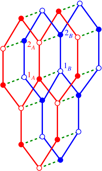
where the index $\alpha=A,B$ labels the two layers. Each site $i$ on each of the two honeycomb layers carries a spin-$s$ particle denoted by the usual SU(2) spin operators ${\bf s}_{i,\alpha}\equiv(s^{x}_{i,\alpha},s^{y}_{i,\alpha},s^{z}_{i,\alpha})$, with ${\bf s}^{2}_{i,\alpha}=s(s+1)$, and where for present purposes we restrict attention to the case $s=\frac{1}{2}$. In Eq. (1) the sums over $\langle i,j\rangle$, $\langle\langle i,k\rangle\rangle$ and $\langle\langle\langle i,l\rangle\rangle\rangle$ run respectively over all NN, NNN and NNNN intralayer bonds on each honeycomb-lattice monolayer, counting each Heisenberg bond once and once only in each sum. The last sum in Eq. (1) describes the interlayer Heisenberg bonds between NN pairs of spins across the two vertically stacked layers. The pattern of bonds is shown in Figs. 1(a) and 1(b).

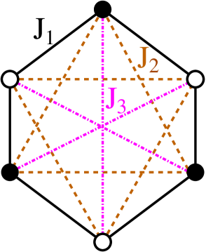
In the present paper we will be interested in the case when all 4 bonds are AFM in nature (i.e., $J_{i}>0,\,i=1,2,3$, and $J_{1}^{\perp}>0$). We will also restrict attention, as discussed in Sec. I, to the particularly interesting case when $J_{3}=J_{2}$. Since we may regard the exchange coupling constant $J_{1}$ as simply setting the overall energy scale, the relevant parameters are thus $(J_{3}/J_{1}=)J_{2}/J_{1}\equiv\alpha$, and $J_{1}^{\perp}/J_{1}\equiv\delta$.

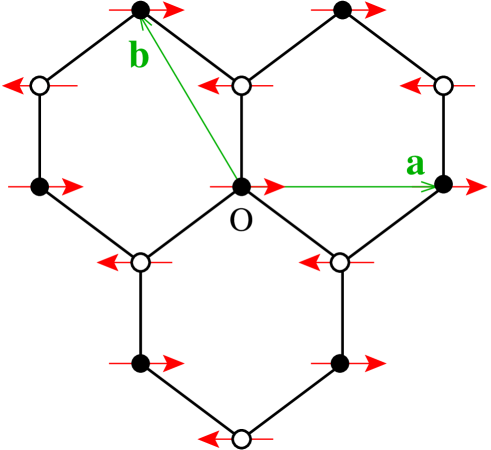
The honeycomb lattice itself is non-Bravais. It has a 2-site unit cell, with two triangular sublattices 1 and 2, and triangular Bravais lattice vectors ${\mathbf{a}}$ and ${\mathbf{b}}$, as shown in Fig. 1(c). In terms of unit vectors $\hat{x}$ and $\hat{z}$ that define the $xz$ plane of the monolayers, we have ${\mathbf{a}}=\sqrt{3}d\hat{x}$ and ${\mathbf{b}}=\frac{1}{2}d(-\sqrt{3}\hat{x}+3\hat{z})$, where $d$ is the NN spacing on the hexagonal lattice. Sites on sublattice 1 are at positions ${\mathbf{R}}_{i}=m{\mathbf{a}}+n{\mathbf{b}}$, where $m,n\in\mathbb{Z}$. Each unit cell $i$ at position vector ${\mathbf{R}}_{i}$ on each layer comprises two sites, one at ${\mathbf{R}}_{i}$ on sublattice 1 and the other at ${\mathbf{R}}_{i}+d\hat{z}$ on sublattice 2. In Fig. 1(a) we also show the corresponding four sites of the $AA$-stacked bilayer unit cell.

In position space the Wigner-Seitz cell for the monolayer is simply the parallelogram formed by the triagonal Bravais lattice vectors ${\mathbf{a}}$ and ${\mathbf{b}}$. Equivalently, it may be chosen to be one of the primitive real-space hexagons of the lattice with side length $d$, centered on a point of sixfold symmetry. In that case, in reciprocal space the first Brillouin zone is then itself also a hexagon, but which is now rotated by 90^∘ with respect to the real-space Wigner-Seitz hexagon, and with side length $4\pi/(3\sqrt{3}d)$. Its first three corners are thus at positions ${\mathbf{K}}^{(1)}=4\pi/(3\sqrt{3}d)\hat{x}$, ${\mathbf{K}}^{(2)}=2\pi/(3\sqrt{3}d)\hat{x}+2\pi/(3d)\hat{z}$, and ${\mathbf{K}}^{(3)}=-2\pi/(3\sqrt{3}d)\hat{x}+2\pi/(3d)\hat{z}$. The remaining three corners are at positions ${\mathbf{K}}^{(i+3)}=-{\mathbf{K}}^{(i)};\;i=1,2,3$.

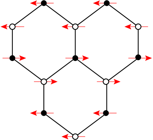
Let us first briefly review the situation for the model under consideration when $\delta=0$ (i.e., for the monolayer). Along the line $J_{3}=J_{2}=\alpha J_{1}$ in the classical case there is a direct transition between the two collinear AFM phases at $\alpha_{{\rm cl}}=\frac{1}{2}$. These are the Néel phase shown in Fig. 1(c), which is the GS phase for $\alpha<\alpha_{{\rm cl}}$, and the striped phase shown in Fig. 1(d), which is the GS phase for $\alpha>\alpha_{{\rm cl}}$. Whereas the Néel phase on the honeycomb-lattice monolayer has all three NN pairs of spins antiparallel to one another at each site, the striped phase has only one NN pair antiparallel and the other two parallel to one another. Equivalently, the striped phase is composed of parallel ferromagnetic zigzag (or sawtooth) chains along one of the three equivalent honeycomb directions, with neighboring chains coupled antiferromagnetically. The striped state shown in Fig. 1(d) thus has two other equivalent states rotated with respect to it by $\pm 120^{\circ}$ in the lattice plane.

As usual, the classical phases may generically be described by an ordering wave vector ${\mathbf{Q}}$, together with a parameter $\theta$ that measures the angle between the two spins in each monolayer unit cell $i$ at position vector ${\mathbf{R}}_{i}$. The classical spins, of length $s$, are thus written as

$${\mathbf{s}}_{i,\rho}=s[\cos({\mathbf{Q}}\cdot{\mathbf{R}}_{i}+\theta_{\rho})\hat{x}_{s}+\sin({\mathbf{Q}}\cdot{\mathbf{R}}_{i}+\theta_{\rho})\hat{z}_{s}]\,,$$

(2)

where the index $\rho$ labels the two sites in the unit cell, and $\hat{x}_{s}$ and $\hat{z}_{s}$ are two orthogonal unit vectors that define the plane of the spins. The angles $\theta_{\rho}$ may be chosen with no loss of generality so that $\theta_{1}=0$ for spins on triangular-sublattice 1 and $\theta_{2}=\theta$ for spins on triangular-sublattice 2. In this description of the classical phases the Néel phase shown in Fig. 1(c) has wave vector ${\mathbf{Q}}=0$ and $\theta=\pi$. Similarly, the striped phase shown in Fig. 1(d) has wave vector ${\mathbf{Q}}={\mathbf{M}}^{(2)}$ and $\theta=\pi$, where ${\mathbf{M}}^{(2)}=2\pi/(3d)\hat{z}$ is the vector of the midpoint of the edge joining the corners of the hexagonal first Brillouin zone at positions ${\mathbf{K}}^{(2)}$ and ${\mathbf{K}}^{(3)}$. The two other inequivalent striped states are hence described by the wave vectors of the remaining inequivalent midpoints of the other two edges of the first Brillouin zone, and in each case now with $\theta=0$. Thus, the other two striped states have wave vectors ${\mathbf{Q}}={\mathbf{M}}^{(1)}=\pi/(\sqrt{3}d)\hat{x}+\pi/(3d)\hat{z}$ (that is the midpoint of the edge joining corners ${\mathbf{K}}^{(1)}$ and ${\mathbf{K}}^{(2)}$), and ${\mathbf{Q}}={\mathbf{M}}^{(3)}=-\pi/(\sqrt{3}d)\hat{x}+\pi/(3d)\hat{z}$ (that is the midpoint of the edge joining corners ${\mathbf{K}}^{(3)}$ and ${\mathbf{K}}^{(4)}$).

Let us now compare this classical result for the monolayer ($\delta=0$) version of our model with the corresponding case when $s=\frac{1}{2}$. In the spin-$\frac{1}{2}$ case the classical transition point is split into two quantum critical points (QCPs) at $\alpha_{c_{1}}<\alpha_{{\rm cl}}$ and $\alpha_{c_{2}}>\alpha_{{\rm cl}}$, with a magnetically disordered paramagnetic GS phase in the intermediate region Cabra et al. (2011); Farnell et al. (2011). Lowest-order spin-wave theory, for example, provides the estimates Cabra et al. (2011) $\alpha_{c_{1}}\approx 0.29$ and $\alpha_{c_{2}}\approx 0.55$. By contrast, the more powerful, and potentially more accurate, method of Schwinger-boson mean-field theory (SBMFT) yields the estimates Cabra et al. (2011) $\alpha_{c_{1}}\approx 0.41$ and $\alpha_{c_{2}}\approx 0.6$. SBMFT also predicts a quantum disordered phase in the intermediate regime $\alpha_{c_{1}}<\alpha<\alpha_{c_{2}}$, where a gap opens up in the bosonic dispersion and the spin-spin correlation function displays traces of Néel short-range order. These results are broadly confirmed by high-order CCM calculations Farnell et al. (2011), which yield the values $\alpha_{c_{1}}\approx 0.47$ and $\alpha_{c_{2}}\approx 0.60$. Furthermore, CCM calculations of the plaquette valence-bond crystalline (PVBC) susceptibility Farnell et al. (2011) provide strong evidence for the intermediate paramagnetic phase to be a gapped state with PVBC order over the entire region.

Of special interest for the spin-$\frac{1}{2}$ monolayer, the QPT at $\alpha_{c_{1}}$ between the Néel phase (that is the stable GS phase for $\alpha<\alpha_{c_{1}}$) and the paramagnetic phase (that is the stable GS phase for $\alpha_{c_{1}}<\alpha<\alpha_{c_{2}}$) appears to be continuous, while that at $\alpha_{c_{2}}$ appears to be of first-order type Farnell et al. (2011). Since the Néel and intermediate phases break different symmetries, the QPT at $\alpha_{c_{1}}$ is thus favored to be described by the scenario of deconfined quantum criticality Senthil et al. (2004a); *Senthil:2004_PRB_deconfinedQC_merge. In view of this rich scenario it seems of considerable interest to study the comparable spin-$\frac{1}{2}$ $J_{1}$–$J_{2}$–$J_{3}$–$J_{1}^{\perp}$ model on the $AA$-stacked honeycomb bilayer, where we now include AFM interlayer NN bonds of strength $J_{1}^{\perp}>0$. Once again we will study the model here along the line $J_{3}=J_{2}\equiv\alpha J_{1}$ with $J_{1}^{\perp}\equiv\delta J_{1}$. Specific goals will be to study how the QCPs $\alpha_{c_{1}}$ and $\alpha_{c_{2}}$ now depend on the interlayer coupling parameter $\delta$. To that end we will use the same theoretical technique, viz., the coupled cluster method (CCM), as has been used previously to describe accurately the corresponding monolayer case ($\delta=0$) Farnell et al. (2011).

Let us now turn to the corresponding case of the $J_{1}$–$J_{2}$–$J_{3}$–$J_{1}^{\perp}$ model (with $J_{3}=J_{2}$), on the $AA$-stacked honeycomb-lattice bilayer, which we aim to study here for the spin-$\frac{1}{2}$ case. At the classical $(s\rightarrow\infty)$ level the inclusion of an NN interlayer coupling with strength $J_{1}^{\perp}>0$ introduces no extra frustration, and its effect is essentially trivial. Simply the NN interlayer pairs of spins anti-align, with each monolayer having the same Néel order for $\alpha<\alpha_{{\rm cl}}$ or striped order for $\alpha>\alpha_{{\rm cl}}$ as in the absence of interlayer pairing. By contrast, as we have discussed in detail in Sec. I, the spin-$\frac{1}{2}$ case is expected to be of greater interest and subtlety, due to the expected formation of NN interlayer spin-singlet dimers in the large-$\delta$ limit, where the GS phase will thus be a valence-bond crystalline (VBC) phase formed from interlayer dimers. This interlayer dimer VBC (IDVBC) phase will be gapped, by contrast to the gapless nature of the quasiclassical Néel and striped phases with magnetic LRO, where the magnon excitations are massless Goldstone modes. In the complete IDVBC phase (i.e., in the limit $\delta\rightarrow\infty$) the lowest-lying excited state is a spin-1 state formed by breaking a single NN interlayer dimer from a spin-singlet to a spin-triplet state. Thus, we expect the scaled triplet spin gap to be given, in the limiting case, by

$$\frac{\Delta}{J_{1}}\xrightarrow[\delta\to\infty]{}\delta\,.$$

(3)

As we have noted above, the phase diagram of the model along the line $\delta=0$ (i.e., for the monolayer) is already a rich one, with two QCPs in the range $0\leq\alpha\leq 1$ of the frustration parameter, with one being continuous (and hence probably of a deconfined quantum critical nature) and the other being of first-order type. Clearly, the enlargement of the model by the addition of the extra parameter $\delta$ can only increase our understanding of the quantum phase diagram, even for the case of the monolayer. In particular, the two QCPs for the limiting case $\delta=0$ now become quantum critical lines (or quantum phase boundary lines) in the $\alpha\delta$ plane. As a foretaste of our overall results, one of our most important findings is that these two phase boundary lines display a marked “avoided crossing” behavior, with both curves consequently exhibiting a distinct reentrant nature. This finding by itself clearly throws new light on the phase diagram of the monolayer ($\delta=0$), as discussed more fully in Secs. IV and V.

In order to examine the effect of interlayer coupling on the QCPs $\alpha_{c_{1}}$ and $\alpha_{c_{2}}$ of the spin-$\frac{1}{2}$ honeycomb-lattice monolayer we will therefore present in Sec. IV results for both the magnetic order parameter (i.e., the average local on-site GS magnetization) $M$ and the triplet spin gap $\Delta$, for each of the Néel and striped quasiclassical phases, as functions of both parameters $\alpha$ and $\delta$. We utilize both perfectly-ordered states as model wave functions, on top of which we include quantum fluctuations in a fully systematic formalism (viz., the CCM), as we first demonstrate in Sec. III. In particular we show how the CCM can be implemented in very high orders in a well-defined and fully systematic approximation hierarchy, to yield sequences of approximants for both $M$ and $\Delta$. We show further how these sequences can then also be extrapolated, in a controlled and stable manner, to the limit where the corresponding wave functions are exact in principle. These extrapolations are the only approximations made. In Sec. IV we will show explicitly how the results for both $M$ and $\Delta$ yield accurate and consistent estimates of the phase boundaries, $\alpha_{c_{1}}(\delta)$ and $\alpha_{c_{2}}(\delta)$, of the Néel and striped GS phases.

The CCM Kümmel et al. (1978); Bishop and Lührmann (1978, 1982); Arponen (1983); Bishop and Kümmel (1987); Arponen et al. (1987); Bartlett (1989); Arponen and Bishop (1991); Bishop (1991, 1998); Zeng et al. (1998); Farnell and Bishop (2004) is one of the very few size-extensive and size-consistent techniques of quantum many-body theory. It thereby provides results in the $N\rightarrow\infty$ limit (where $N$ is the number of particles, i.e., lattice spins in our case) from the outset, at all levels of approximation. Hence, no finite-size scaling is ever required. Particularly apposite to the CCM also is the fact that both the Goldstone linked-cluster theorem and the very important Hellmann-Feynman theorem are also preserved at every level of approximate implementation of the formalism. The latter plays a large part in ensuring that the method yields accurate, self-consistent, and robust results for a variety of physical parameters for a given system. The method has been applied very widely, yielding results of great (and often unsurpassed) accuracy to systems as diverse as finite nuclei Kümmel et al. (1978), the electron gas (or jellium) Bishop and Lührmann (1978, 1982), atoms and molecules of interest in quantum chemistry Bartlett (1989), and a broad spectrum of spin-lattice problems of interest in quantum magnetism Farnell et al. (2014); Bishop and Li (2017); Zeng et al. (1998); Farnell and Bishop (2004); Bishop et al. (1994); Zeng et al. (1995, 1996); Bishop et al. (2000); Krüger et al. (2000); Farnell et al. (2001); Darradi et al. (2005); Bishop et al. (2008a, b, 2009, 2010a, 2010b); Bishop and Li (2011); Li and Bishop (2012); Li et al. (2012b, c); Bishop et al. (2012, 2013); Richter et al. (2015); Bishop and Li (2015); Bishop et al. (2015); Bishop and Li (2016); Li et al. (2016); Li and Bishop (2016, 2018).

To initiate the CCM in practice one needs to choose a suitable model (or reference) state to act as a generalized vacuum state. The quantum correlations present in the exact GS or excited-state (ES) wave function of the system are then systematically incorporated on top of the model state in a hierarchical scheme that becomes exact in some limit, which is usually unattainable at particular levels of computational implementation. Appropriate conditions for a state to be a suitable CCM model state have been discussed extensively in the literature Arponen (1983); Arponen et al. (1987); Bishop (1991, 1998); Zeng et al. (1998); Farnell and Bishop (2004). For spin-lattice models, however, all (quasi)classical states with perfect magnetic LRO are suitable CCM model states. Hence, we use here both the Néel and striped states shown in Figs. 1(c) and 1(d) respectively, for each honeycomb-lattice monolayer, in each case with NN interlayer spins on the $AA$-stacked bilayer aligned antiparallel to each other, as our two choices for CCM model state. We will present independent sets of results in Sec. IV based on both model states taken separately.

We shall only briefly review here some of the principal features and most important elements of the CCM, and refer the reader to Refs. Bishop and Li (2017); Kümmel et al. (1978); Bishop and Lührmann (1978, 1982); Arponen (1983); Bishop and Kümmel (1987); Arponen et al. (1987); Bartlett (1989); Arponen and Bishop (1991); Bishop (1991, 1998); Zeng et al. (1998); Farnell and Bishop (2004) for a fuller description. It is very convenient to be able to treat each lattice spin in each model state as being equivalent to one another. A simple way to do so is to perform a separate passive rotation of each such spin so that they all point in the same direction, say downwards (i.e., along the local negative $z_{s}$ axis), in its own local spin-coordinate frame. Accordingly, after such a choice of local spin-coordinate frames has been made, each model state takes the universal form $|\Phi\rangle=|\downarrow\downarrow\downarrow\cdots\downarrow\rangle$. Naturally, the Hamiltonian also needs to be rewritten appropriately for each such choice.

For a completely general quantum many-body system, its exact GS energy eigenket $|\Psi\rangle$, where $H|\Psi\rangle=E|\Psi\rangle$, is expressed in the exponentiated form,

$$|\Psi\rangle={\rm e}^{S}|\Phi\rangle\,;\quad S=\sum_{I\neq 0}{\cal{S}}_{I}C_{I}^{+}\,,$$

(4)

that is a hallmark of the CCM. Its GS energy eigenbra counterpart $\langle\tilde{\Psi}|$, where $\langle\tilde{\Psi}|H=E\langle\tilde{\Psi}|$, is correspondingly expressed in the CCM parametrization,

$$\langle\tilde{\Psi}|=\langle\Phi|\tilde{S}{\rm e}^{-S}\,;\quad\tilde{S}=1+\sum_{I\neq 0}{\cal{\tilde{S}}}_{I}C_{I}^{-}\,,$$

(5)

where $C_{I}^{-}\equiv(C_{I}^{+})^{\dagger}$, and $C_{0}^{+}\equiv 1$, the identity operator. The set-index $I$ here represents a multiparticle configuration, such that the set of states $\{C_{I}^{+}|\Phi\rangle\}$ completely spans the many-body Hilbert space. The model state $|\Phi\rangle$ and the complete set of mutually commuting, multiconfigurational creation operators $\{C_{I}^{+}\}$ must be chosen so that the former is a fiducial vector (or generalized vacuum state) with regard to the latter, in the sense that they obey the conditions,

$$\langle\Phi|C_{I}^{+}=0=C_{I}^{-}|\Phi\rangle\,,\quad\forall I\neq 0\,,$$

(6)

as well as

$$[C_{I}^{+},C_{J}^{+}]=0\,,\quad\forall I,J\,.$$

(7)

The model state $|\Phi\rangle$ is chosen to be normalized, $\langle\Phi|\Phi\rangle\equiv 1$, and the CCM parametrization of Eq. (4) ensures that the exact GS wave function $|\Psi\rangle$ obeys the intermediate normalization condition, $\langle\Phi|\Psi\rangle=1$. Similarly, the CCM parametrization of Eq. (5) for $\langle\tilde{\Psi}|$ ensures the automatic fulfillment of the normalization condition $\langle\tilde{\Psi}|\Psi\rangle=1$. In practice, it is also convenient to orthonormalize the set of states $\{C_{I}^{+}|\Phi\rangle\}$, i.e., so that they obey the relations,

$$\langle\Phi|C_{I}^{-}C_{J}^{+}|\Phi\rangle=\delta_{I,J}\,,\quad\forall I,J\neq 0\,,$$

(8)

where $\delta_{I,J}$ is a suitably generalized Kronecker symbol.

We note that Hermiticity clearly ensures that the destruction correlation operator $\tilde{S}$ may formally be expressed in terms of its creation counterpart $S$ via the relation

$$\langle\Phi|\tilde{S}=\frac{\langle\Phi|{\rm e}^{S^{\dagger}}{\rm e}^{S}}{\langle\Phi|{\rm e}^{S^{\dagger}}{\rm e}^{S}|\Phi\rangle}\,.$$

(9)

A key feature of the CCM is that the constraint of Eq. (9) is not imposed explicitly. Rather, the operator $\tilde{S}$ is formally decomposed independently of $S$, as in Eq. (5). Naturally, in the exact limit, when all multiconfigurational clusters specified by the complete set $\{I\}$ are retained, Eq. (9) would be exactly fulfilled. In practice, when approximations are made to restrict the set $\{I\}$ to some manageable subset, Eq. (9) may only be approximately fulfilled. This manifest loss of Hermiticity, however, is more than compensated by the gain that the Hellmann-Feynman theorem is itself exactly fulfilled by the CCM parametrizations of Eqs. (4) and (5), even when the sums over the multiconfigurational indices $\{I\}$ are restricted.

Turning now to the specific case of a quantum spin-lattice system, in the local spin-coordinate frames discussed above, where the CCM model state takes the universal form $|\Phi\rangle=|\downarrow\downarrow\downarrow\cdots\downarrow\rangle$, the operator $C_{I}^{+}$ can now also be chosen to have the universal form of a product of single-spin raising operators, $s_{k}^{+}\equiv s_{k}^{x}+is_{k}^{y}$. Thus, the set-index $I$ now takes the form of a set of site indices,

$$I\equiv\{k_{1},k_{2},\cdots,k_{n}\,;\quad n=1,2\cdots 2sN\}\,,$$

(10)

in which no given site index $k_{i}$ may appear more than 2$s$ times. Correspondingly, the operator $C_{I}^{+}$ creates a multispin configuration cluster,

$$C^{+}_{I}\equiv s^{+}_{k_{1}}s^{+}_{k_{2}}\cdots s^{+}_{k_{n}};\;\quad n=1,2,\cdots 2sN\,.$$

(11)

Clearly, all the GS quantities may now be expressed wholly in terms of the CCM correlation coefficients $\{{\cal S}_{I},\tilde{{\cal S}}_{I}\}$. For example, the GS magnetic order parameter, which is simply the average local on-site magnetization, takes the form

$$M=-\frac{1}{N}\langle\Phi|\tilde{S}\sum_{k=1}^{N}{\rm e}^{-S}s_{k}^{z}{\rm e}^{S}|\Phi\rangle\,,$$

(12)

where $s_{k}^{z}$ is expressed in the local rotated spin axes described above. Thus, all that remains for the GS calculations is to calculate the coefficients $\{{\cal S}_{I},\tilde{{\cal S}}_{I}\}$.

Formally, this is done by minimizing the GS energy expectation functional,

$$\bar{H}=\bar{H}[{\cal S}_{I},{\tilde{\cal S}_{I}}]\equiv\langle\Phi|\tilde{S}{\rm e}^{-S}H{\rm e}^{S}|\Phi\rangle\,,$$

(13)

with respect to all coefficients $\{{\cal S}_{I},{\tilde{\cal S}}_{I}\,;\forall I\neq 0\}$. Extremization with respect to $\tilde{{\cal S}}_{I}$, using Eq. (5), trivially yields the relations

$$\langle\Phi|C^{-}_{I}{\rm e}^{-S}H{\rm e}^{S}|\Phi\rangle=0\,,\quad\forall I\neq 0\,,$$

(14)

which are a coupled set of nonlinear equations for the coefficients $\{{\cal S}_{I}\}$. Similarly, use of Eq. (4) and extremization of $\bar{H}$ with respect to ${\cal S}_{I}$, yields the relations

$$\langle\Phi|\tilde{S}({\rm e}^{-S}H{\rm e}^{S}-E)C^{+}_{I}|\Phi\rangle=0\,,\quad\forall I\neq 0\,,$$

(15)

where we have also used the simple relation $[S,C_{I}^{+}]=0$, which follows from the explicit CCM parametrization of Eq. (4) together with Eq. (7). Equation (15) is just a set of linear equations for the coefficients $\{\tilde{{\cal S}}_{I}\}$, once the coefficients $\{{\cal S}_{I}\}$ are input, having first been obtained by solving Eq. (14).

An ES energy eigenket $|\Psi_{e}\rangle$, where $H|\Psi_{e}\rangle=E_{e}|\Psi_{e}\rangle$ is similarly expressed in the CCM formalism in terms of a linear excitation operator, $X^{e}$, as

$$|\Psi_{e}\rangle=X^{e}{\rm e}^{S}|\Phi\rangle\,;\quad X^{e}=\sum_{I\neq 0}{\cal X}_{I}^{e}C_{I}^{+}\,,$$

(16)

as the analog of Eq. (4) for the GS counterpart. Using the obvious commutativity relation, $[X^{e},S]=0$, which follows from Eqs. (4), (7), and (16), it is easy to combine the GS and ES Schrödinger equations to yield the equation

$$e^{-S}[H,X^{e}]e^{S}|\Phi\rangle=\Delta_{e}X^{e}|\Phi\rangle\,,$$

(17)

where $\Delta_{e}$ is the excitation energy,

$$\Delta_{e}\equiv E_{e}-E\,.$$

(18)

By taking the inner product of Eq. (17) with $\langle\Phi|C_{I}^{-}$, and making use of Eq. (8), one may readily derive the set of equations,

$$\langle\Phi|C_{I}^{-}({\rm e}^{-S}H{\rm e}^{S}-E)X^{e}|\Phi\rangle=\Delta_{e}{\cal X}_{I}^{e}\,,\quad\forall I\neq 0\,.$$

(19)

Once the operator $({\rm e}^{-S}H{\rm e}^{S}-E)$ has been input into Eq. (19) from the solution to Eq. (14), Eq. (19) is simply a set of generalized linear eigenvalue equations for the ES ket-state CCM correlation coefficients $\{{\cal X}_{I}^{e}\}$ and the excitation energy (eigenvalue) $\Delta_{e}$.

Everything so far has been formally exact, and we turn now to where approximations may be needed for computational implementation of the CCM formalism. One possible source of approximation could involve the evaluation of the exponentiated operators ${\rm e}^{\pm S}$ that lie at the heart of the CCM parametrizations of Eqs. (4), (5), and (16). However, we note that in each of Eqs. (14), (15), and (19) that need to be solved for the CCM correlation coefficients $\{{\cal S}_{I}\}$, $\{{\tilde{\cal S}}_{I}\}$ and $\{{\cal X}_{I}^{e}\}$, these appear only in the combination ${\rm e}^{-S}H{\rm e}^{S}$ of a similarity transform of the system Hamiltonian. We have described in detail elsewhere (and see, e.g., Refs. Farnell and Bishop (2004); Bishop et al. (2015); Li and Bishop (2016) and references cited therein) how the otherwise infinite-order nested commutator expansion

$${\rm e}^{-S}H{\rm e}^{S}=\sum_{n=0}^{\infty}\frac{1}{n!}[H,S]_{n}\,,$$

(20)

where $[H,S]_{n}$, the $n$-fold nested commutator, is defined iteratively as

$$[H,S]_{n}\equiv[[H,S]_{n-1},S]\,;\quad[H,S]_{0}=H\,,$$

(21)

actually terminates exactly in the present case at the term with $n=2$. Similarly, all GS expectation values, such as the magnetic order parameter $M$ of Eq. (12) may be evaluated without any truncations of the similarity transform ${\rm e}^{-S}s_{k}^{z}{\rm e}^{S}$.

Hence, the sole approximation made is in the choices of which subsets of multispin-flip configurations $\{I\}$ to retain in the expansions of correlation coefficients for both the GS wave functions, as in Eqs. (4), (5), and the ES wave function considered, as in Eq. (16). In the present case we restrict attention to the lowest-lying spin-triplet excitation, so that $\Delta_{e}$ now becomes equal to the spin-triplet gap, which we denote by $\Delta$. For both the GS and ES calculations we employ the well-known lattice animal-based subsystem (LSUB$n$) truncation hierarchy, which has been much studied and utilized for a wide variety of spin-lattice problems in the past (and see e.g., Refs. Farnell et al. (2014); Bishop and Li (2017); Farnell et al. (2011); Li et al. (2012a); Zeng et al. (1998); Farnell and Bishop (2004); Li and Bishop (2016) and references cited therein).

At the LSUB$n$ level of approximation one retains all multispin-flip configurations $I$ in the CCM correlation operators ${\cal S}$, $\tilde{{\cal S}}$ and ${\cal X}^{e}$ defined in Eqs. (4), (5), and (16), respectively, which are restrained to all distinct locales on the lattice that contain no more than $n$ contiguous sites. A cluster of sites is said to be contiguous (or to form a lattice animal or polyomino) when each site of the cluster is NN to at least one other, taking into account the geometrical definition of NN sites employed. For the GS calculation we restrict the multispin-flip configurations at each LSUB$n$ level to have $s_{T}^{z}=0$, where $s_{T}^{z}\equiv\sum_{k=1}^{N}s_{k}^{z}$, defined in the global spin axes (i.e., before the local rotations discussed above have been performed). Similarly, for the ES calculation of the triplet spin gap $\Delta$, we restrict the comparable configurations to have $s_{T}^{z}=1$. In both cases we utilize the space- and point-group symmetries of the Hamiltonian and the CCM model state $|\Phi\rangle$ being employed to reduce the number of fundamentally distinct configurations to a minimum, $N_{f}(n)$. Since the number $N_{f}(n)$ increases rapidly as a function of truncation index $n$, it soon becomes necessary to use supercomputing resources and massive parallelization, together with custom-made computer-algebraic packages, to enumerate the independent cluster configurations retained and to derive the corresponding CCM equations at a given LSUB$n$ level, and then finally to solve them Zeng et al. (1998); ccm . For the present bilayer model we are thereby able to perform both the GS and ES calculations reported in Sec. IV at LSUB$n$ levels of approximation with $n\leq 10$. For the GS calculation we have $N_{f}(10)=70\,118$ $(175\,223)$ using the bilayer Néel (striped) states described previously as CCM model states. For the corresponding ES calculation of $\Delta$ we have $N_{f}(10)=121\,103$ $(320\,476)$ using the bilayer Néel (striped) states as CCM model states. Both numbers are larger for the striped state than the Néel state since the former has less symmetries than the latter. We note that for this model the geometric definition of contiguous sites for the LSUB$n$ configurations simply corresponds to NN pairs connected by $J_{1}$ or $J_{1}^{\perp}$ bonds.

Finally, to obtain estimates for our results in the formally exact limit, $n\rightarrow\infty$, we need to extrapolate the raw LSUB$n$ data. Such extrapolations thereby comprise the sole approximation that we make. While exact extrapolation rules are not known, much practical experience from applications of the LSUB$n$ hierarchy to many different spin-lattice models, has shown the widespread accuracy of the consistent use of rather simple schemes for the relevant physical parameters. In this respect the magnetic order parameter $M$ is of special interest, since two different schemes have been employed for differing situations.

Thus, for unfrustrated spin systems or for ones with only small amounts of frustration, an appropriate extrapolation scheme is found to be Li et al. (2012b); Bishop et al. (2012); Bishop and Li (2012); Bishop et al. (2013); Farnell et al. (2014); Bishop et al. (2000); Krüger et al. (2000); Farnell et al. (2001); Darradi et al. (2005); Bishop et al. (2009, 2010a, 2010b); Bishop and Li (2011, 2017)

$$M(n)=m_{0}+m_{1}n^{-1}+m_{2}n^{-2}\,,$$

(22)

from fits to which we obtain the extrapolated LSUB$\infty$ value $m_{0}$ for $M$. By contrast, a more appropriate scheme for systems that exhibit a GS order-disorder QPT, or for phases whose order parameter $M$ is zero or small, is Farnell et al. (2011); Li et al. (2012b); Bishop et al. (2012); Bishop and Li (2012); Li et al. (2012a); Bishop et al. (2013); Li et al. (2016); Li and Bishop (2016); Farnell et al. (2014); Bishop et al. (2008a, b); Li et al. (2012c); Bishop and Li (2017); Li and Bishop (2018)

$$M(n)=\mu_{0}+\mu_{1}n^{-1/2}+\mu_{2}n^{-3/2}\,,$$

(23)

which yields the respective LSUB$\infty$ extrapolant $\mu_{0}$ for $M$.

For the triplet spin gap $\Delta$ an extrapolation scheme with leading power of $n^{-1}$, like that in Eq. (22) for $M$, has been found to give a very good fit to the LSUB$n$ approximants $\Delta(n)$ for both of the above cases of unfrustrated (or slightly frustrated) and highly frustrated systems Li and Bishop (2016); Bishop et al. (2015); Krüger et al. (2000); Richter et al. (2015); Bishop and Li (2015, 2017); Li and Bishop (2018),

$$\Delta(n)=d_{0}+d_{1}n^{-1}+d_{2}n^{-2}\,,$$

(24)

from fits to which we obtain the extrapolated LSUB$\infty$ estimate $d_{0}$ for $\Delta$.

Clearly, for each of the fits of Eqs. (22)–(24), it is best to use four or more fitting points (i.e., different $n$ values of the LSUB$n$ sequence) to obtain robust and the most reliable results. Furthermore, the LSUB2 result is expected, a priori to be too close to mean-field theory and too far from the exact $n\rightarrow\infty$ limit to be used in each fit, if it can be avoided. For this reason, our preferred sets of LSUB$n$ approximants for the fits are those with $n=\{4,6,8,10\}$ in the present case where it is computationally infeasible to calculate results for $n>10$.

We also note, however, that a $(4m-2)/4m$ staggering effect, where $m\in\mathbb{Z}^{+}$ is a positive integer, has been observed Bishop et al. (2012, 2013); Li and Bishop (2016) in LSUB$n$ sequences of CCM results for various physical parameters on frustrated honeycomb-lattice monolayers. Such staggering implies that the two sub-sequences with $n=4m-2$ and with $n=4m$ need to be extrapolated separately from one another. In some cases corresponding adjacent pairs of curves from each sub-sequence (e.g., those with $n=2$ and $n=4$, or with $n=6$ and $n=8$) even cross one another as some coupling parameter is varied. Such staggering has been possibly attributed Li and Bishop (2016) to the fact that the honeycomb lattice comprises two interlocking triangular Bravais lattices, on each of which a more well-known $(2m-1)/2m$ (i.e., odd/even) staggering effect is commonly seen, exactly analogous to the same effect that is well understood in perturbation theory. Indeed, this is precisely the reason why LSUB$n$ results with odd values of the truncation index $n$ are not included in our CCM extrapolations here. In view of these prior observations on frustrated honeycomb-lattice monolayers, we shall also compare our results in Sec. IV between extrapolations based on the preferred sequences with $n=\{4,6,8,10\}$ and those based on $n=\{2,6,10\}$. The latter sequence is sub-optimal in the two aspects that it both includes the LSUB2 result and is based on only three fitting points to extract three parameters. Nevertheless, it avoids mixing results from the two staggered sub-sequences.

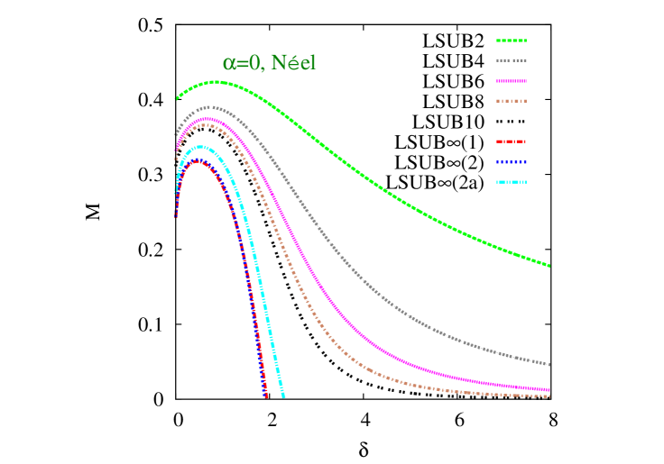
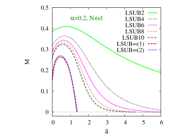
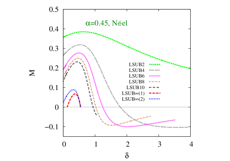
We first show in Fig. 2 our CCM results for the GS magnetic order parameter $M$ of Eq. (12) in the Néel phase, as a function of the scaled interlayer exchange coupling constant, $\delta\equiv J_{1}^{\perp}/J_{1}$, for three particular representative values of the intralayer frustration parameter, $\alpha\equiv J_{2}/J_{1}$. In each case we show the “raw” LSUB$n$ data with $n=2,4,6,8,10$, based on the Néel state of Fig. 1(c) as the CCM model state, together with various LSUB$\infty$ extrapolations. We note in particular that the two extrapolations based on the scheme of Eq. (23), but using the two respective LSUB$n$ data sets with $n=\{2,6,10\}$ and $n=\{4,6,8,10\}$ give results in very close agreement with one another for all three values of $\alpha$ shown and for most values of $\delta$. Generally, the only exception, where there is some slight sensitivity to the extrapolation input data is the joint region of the highest values of intralayer frustration (near to where Néel order disappears) and the lowest values of interlayer AFM coupling, as seen in Fig. 2(c), for example.

It is interesting to note that in each case the effect of turning on the interlayer coupling is first to enhance the stability of the Néel order, up to some particular value of $\delta$, which depends on the intralayer frustration parameter $\alpha$. Increasing $\delta$ beyond this value then leads to a decrease in the Néel order parameter $M$, out to some critical value $\delta_{c_{1}}^{>}(\alpha)$ at which $M\rightarrow 0$. Furthermore, we note that Néel order persists in the honeycomb-lattice monolayer $(\delta=0)$ for all values of the frustration parameter in the range $\alpha<\alpha_{c_{1}}(0)$. In this range we find an upper critical value $\delta_{c_{1}}^{>}(\alpha)$ of the scaled interlayer exchange coupling constant, such that Néel order persists over the range $0<\delta<\delta_{c_{1}}^{>}(\alpha)$. Very interestingly, however, as may be seen from Fig. 2(c), for example, for higher values of $\alpha$ in the range $\alpha_{c_{1}}(0)<\alpha<\alpha_{1}^{>}$, we find a reentrant type of behavior in which Néel order now exists only over the range $\delta_{c_{1}}^{<}(\alpha)<\delta<\delta_{c_{1}}^{>}(\alpha)$, with $\delta_{c_{1}}^{<}(\alpha)>0$. The corresponding upper and lower critical values coincide when $\alpha=\alpha_{1}^{>}$, at which point, we thus have $\delta_{c_{1}}^{<}(\alpha_{1}^{>})=\delta_{c_{1}}^{>}(\alpha_{1}^{>})$. Finally, Néel order is absent for $\alpha>\alpha_{1}^{>}$, for all values of $\delta$.

The extrapolation scheme of Eq. (23), used for the LSUB$\infty(1)$ and LSUB$\infty(2)$ results shown in each of Figs. 2(a), 2(b), and 2(c), is certainly valid for all these cases when the frustration is appreciable, especially for systems close to a QCP as here, at which the magnetic order parameter vanishes. However, for unfrustrated systems or ones that are only slightly unfrustrated, the scheme of Eq. (22) provides a better fit to the LSUB$n$ input data. Accordingly, we also show in Fig. 2(a) alone the LSUB$\infty(2a)$ extrapolation based on Eq. (22) and the input data set $n=\{4,6,8,10\}$. This extrapolation is then valid for this case of zero intralayer frustration $(\alpha=0)$ only for a small range of values of the scaled interlayer coupling, $\delta\lesssim 0.2$, say.

In particular, the LSUB$\infty(2a)$ curve gives a value $M=0.2741(1)$ for the unfrustrated honeycomb-lattice monolayer (i.e., with $\alpha=0=\delta$), where the quoted error is simply the least-squares error associated with the fit. The corresponding result using Eq. (22) and the input data set $n=\{2,6,10\}$ is $M=0.2761$. There is clearly a small sensitivity associated with the LSUB$n$ input data set used of about $1\%$ or so. In this case $(\alpha=0=\delta)$ alone, where “minus-sign problems” are absent, we may compare our CCM results with recent values obtained from two different quantum Monte Carlo (QMC) simulations, which yielded the corresponding respective values $M=0.2681(8)$ Löw (2009) and $M=0.26882(3)$ Jiang (2012). The agreement with our own CCM estimates is very good, and we expect a corresponding accuracy (i.e., of the order of $2\%$) for all the results that we present. Indeed, for the monolayer case, where we are also able to perform LSUB$n$ calculations with $n=12$, our corresponding extrapolated value, based on the data set $n=\{8,10,12\}$, again with only three fitting points, for example, is $M=0.2715$, in even better agreement $(1\%)$ with the QMC result.

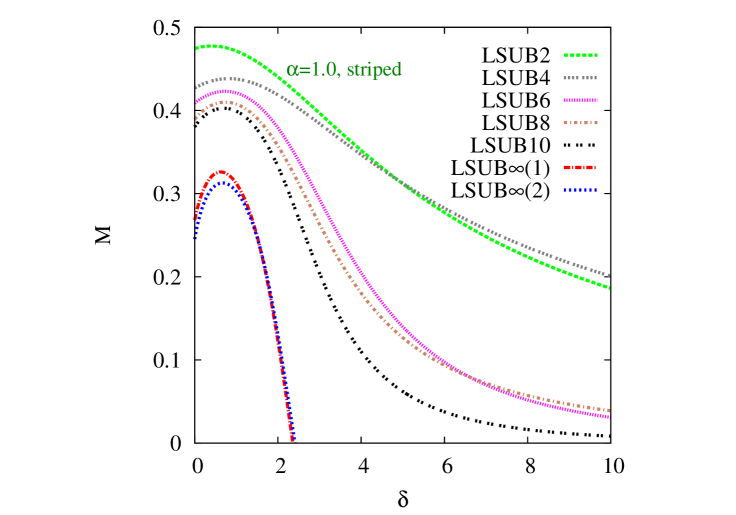
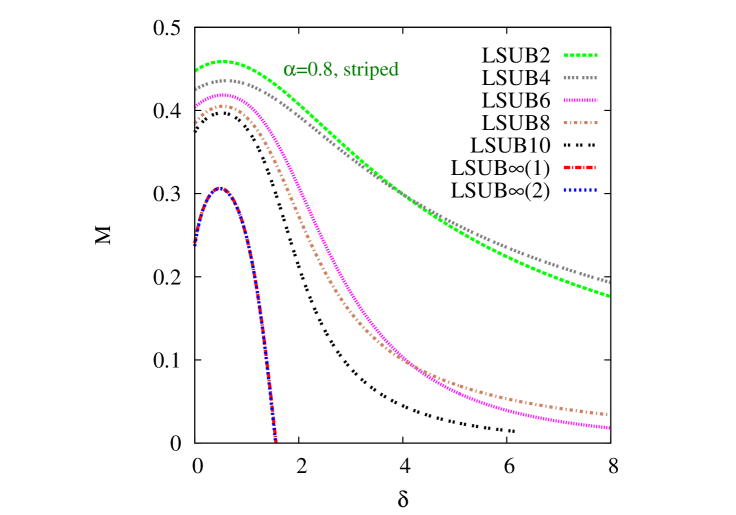
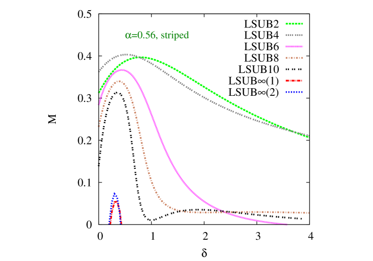
In Fig. 3 we show corresponding results for the GS magnetic order parameter $M$ of Eq. (12) in the striped phase to those shown in Fig. 2 for the Néel phase. Again, we show results for $M(\delta)$ for three particular representative values of the intralayer frustration parameter $\alpha$. In each case we show the same “raw” LSUB$n$ data with $n=2,4,6,8,10$, but now based on the striped state of Fig. 1(d) as the CCM model state. We also display in Fig. 3 the same LSUB$\infty(1)$ and LSUB$\infty(2)$ extrapolations as those shown in Fig. 2, both of which are based on the appropriate scheme of Eq. (23), but with the two respective LSUB$n$ input data sets $n=\{2,6,10\}$ and $n=\{4,6,8,10\}$.

Again, we note that the two extrapolations are in remarkable agreement with each other in every case, despite the $(4m-2)/4m$ staggering that has been discussed in Sec. III and which is now clearly visible in each of Figs. 3(a), 3(b), and 3(c), where it manifests itself most vividly as actual crossings of corresponding adjacent pairs of curves (viz., LSUB2 and LSUB4, corresponding to $m=1$, and LSUB6 and LSUB8, corresponding to $m=2$). Presumably, the very close agreement between the LSUB$\infty(1)$ and LSUB$\infty(2)$ extrapolations, the former of which takes the staggering into account and the latter of which does not, is related to the fact that the crossings occur only for unphysical values of $\delta$, far beyond the associated QCP at which the (extrapolated) striped order parameter has vanished.

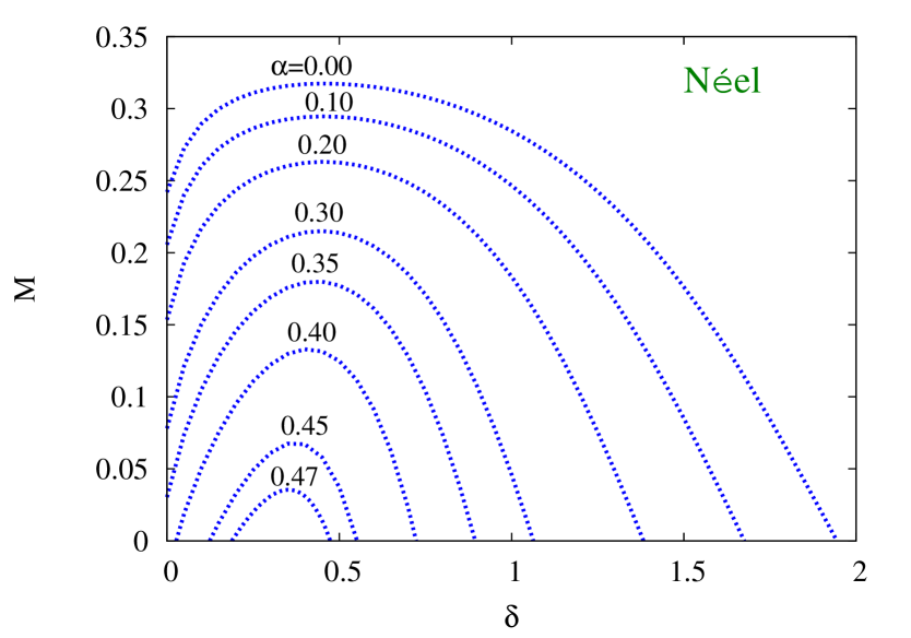
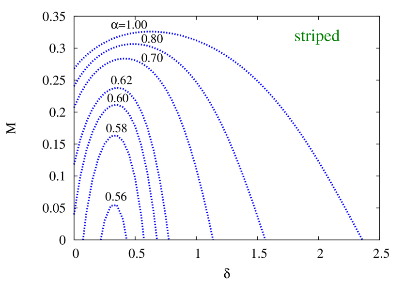
Figure 3 exhibits a reentrant behavior very similar to that seen in Fig. 2, and discussed above, for the Néel phase. Thus, striped order is present in the honeycomb-lattice monolayer $(\delta=0)$ for all values of the intralayer frustration parameter in the range $\alpha>\alpha_{c_{2}}(0)$. In this range we observe from Fig. 3 that as the AFM bilayer coupling is turned on, striped order persists over the range $0<\delta<\delta_{c_{2}}^{>}(\alpha)$ of the scaled interlayer exchange coupling. However, now for somewhat lower values of $\alpha$ in the range $\alpha_{2}^{<}<\alpha<\alpha_{c_{2}}(0)$, we again observe a reentrant behavior in which striped order reappears over the range $\delta_{c_{2}}^{<}(\alpha)<\delta<\delta_{c_{2}}^{>}(\alpha)$, with $\delta_{c_{2}}^{<}(\alpha)>0$. Similar to the Néel case, these respective upper and lower critical values for the striped phase coalesce when $\alpha=\alpha_{2}^{<}$, such that $\delta_{c_{2}}^{<}(\alpha_{2}^{<})=\delta_{c_{2}}^{>}(\alpha_{2}^{<})$. Striped order is then absent for all values of $\delta$ for $\alpha<\alpha_{2}^{<}$.

The reentrant behavior for both the Néel and striped phases is also demonstrated more graphically in Fig. 4. Here we show sequences of extrapolated results for the magnetic order parameter of both phases as functions of $\delta$, for a variety of values of $\alpha$ in both cases. All of the extrapolations shown are based on the scheme of Eq. (23), used with the corresponding LSUB$n$ input data sets with $n=\{2,6,10\}$. With this particular extrapolation the two QCPs for the monolayers are $\alpha_{c_{1}}(0)\approx 0.379$ and $\alpha_{c_{2}}(0)\approx 0.595$. These may be compared, for example, with the corresponding results Cabra et al. (2011), $\alpha_{c_{1}}(0)\approx 0.41$ and $\alpha_{c_{2}}(0)\approx 0.6$, from using a rotationally-invariant version of Schwinger boson mean-field theory, which has proven itself to be a fairly accurate technique for taking quantum fluctuations into account. By contrast, lowest-order (or linear) spin-wave theory gives the less accurate results Cabra et al. (2011), $\alpha_{c_{1}}(0)\approx 0.29$ and $\alpha_{c_{2}}(0)\approx 0.55$. Our own corresponding CCM results for $\alpha_{1}^{>}$ and $\alpha_{2}^{<}$ are $\alpha_{1}^{>}\approx 0.487$ and $\alpha_{2}^{<}\approx 0.556$, again based on the extrapolation scheme of Eq. (23) used with the LSUB$n$ input data set with $n=\{2,6,10\}$.

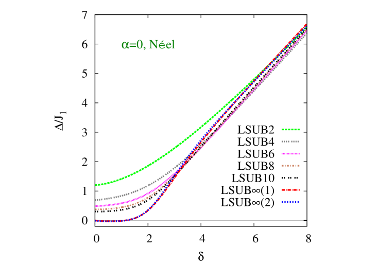
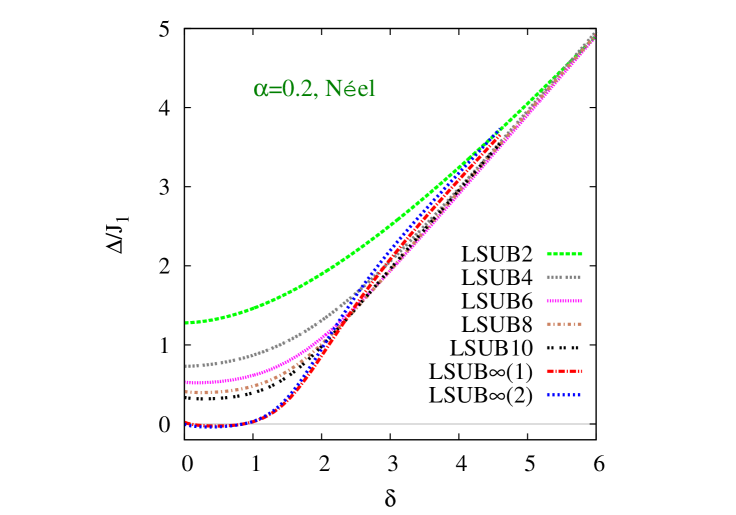
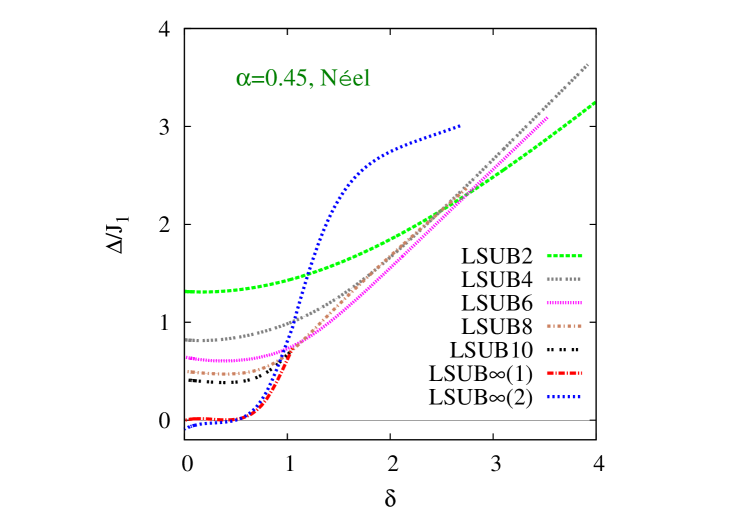
We turn now to our respective results for the triplet spin gap $\Delta$. We first show in Fig. 5 results based on the Néel state as our CCM model state as a function of the scaled interlayer exchange coupling constant, $\delta\equiv J_{1}^{\perp}/J_{1}$, for the same three representative values of the intralayer frustration parameter, $\alpha\equiv J_{2}/J_{1}$, as were shown in Fig. 2 for the GS magnetic order parameter $M$. We note that the two sets of extrapolations, now both based on Eq. (24) but using the two LSUB$n$ input data sets with $n=\{2,6,10\}$ and $n=\{4,6,8,10\}$, are in excellent agreement with one another. Both give results for $\Delta$ that are zero, within very small numerical errors, when Néel order is present, as expected, i.e., for $\delta<\delta_{c_{1}}^{>}(\alpha)$. Furthermore, the values obtained for $\delta_{c_{1}}^{>}(\alpha)$ are in good agreement with the independent values obtained from Fig. 2 for where the GS magnetic order parameter $M$ vanishes. It is clear too that in each case the non-magnetic phase that opens up after the melting of Néel order is gapped, consistent with it having a VBC character.

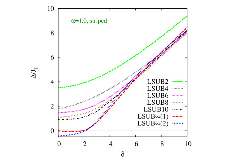
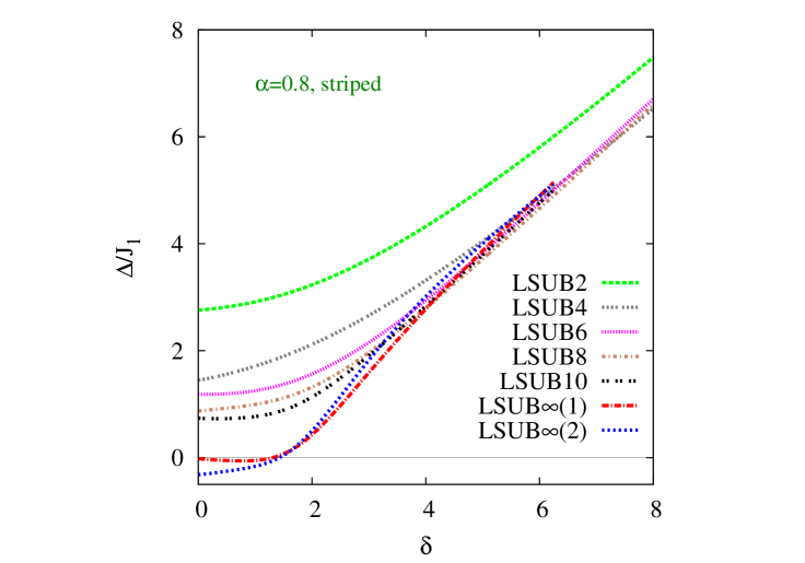
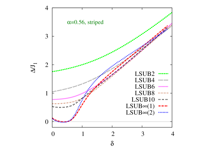
Our corresponding CCM results for the triplet spin gap $\Delta$ based on the striped state as the model state are shown in Fig. 6. Once again we display results as a function of $\delta$, now for the same three representative values of $\alpha$ as were shown in Fig. 3 for the magnetic order parameter $M$. In this case the extrapolated LSUB$\infty(1)$ results, based on the input LSUB$n$ data set $n=\{2,6,10\}$, give results that $\Delta$ is zero, within extremely small numerical errors, for all three values of $\alpha$ shown, over essentially the same ranges of values of $\delta$, viz., $0<\delta<\delta_{c_{2}}^{>}(\alpha)$ for $\alpha>\alpha_{c_{2}}(0)$ and $\delta_{c_{2}}^{<}<\delta<\delta_{c_{2}}^{>}(\alpha)$ for $\alpha_{2}^{<}<\alpha<\alpha_{c_{2}}(0)$, for which the striped magnetic order parameter $M$ is positive in Fig. 3. By contrast, for the striped state, the LSUB$\infty(2)$ extrapolation, based on the input LSUB$n$ data set with $n=\{4,6,8,10\}$, is definitely not as accurate or reliable as the LSUB$\infty(1)$ extrapolation in this respect. This is surely due now to the $(4m-2)/4m$ staggering effect that is clearly visible in the LSUB$n$ sequences of results shown in Fig. 6(a)–(c).

By way of further elucidation of the extrapolation of sequences of approximants that display a staggering as in Fig. 6, it is instructive to consider an analogous situation in $n$th-order perturbation theory (PT), for which exact extrapolation laws can be derived for various physical quantities. However, as is very well known, the even ($n=2m$, where $m\in\mathbb{Z}^{+}$) and odd ($n=2m-1$) sequences of PT approximants involve an additional staggering effect, exactly as is also seen in corresponding CCM LSUB$n$ approximants. In both cases the even and odd sequences obey an extrapolation scheme of the same sort (i.e., with the same leading exponent), but one should not mix even and odd terms together in a single approximation scheme, unless the staggering is incorporated somehow, since the coefficients are not identical for both sequences. The explicit inclusion of the staggering is always very difficult to achieve in a robust manner, and hence in practice one always extrapolates only the even-order terms or the odd-order terms, as mentioned in Sec. III. For honeycomb-lattice models of the sort considered here, it has been observed previously, as discussed above, that there is an additional staggering in the even-order sequence of LSUB$n$ terms between those with $n=4m$ and those with $n=4m-2$. This staggering can clearly be seen by visual inspection of the LSUB$n$ curves shown in Fig. 6. Once again, both subsequences still separately obey Eq. (24). If we do, however, despite the staggering, mix terms from the latter two subsequences, as in our LSUB$\infty(2)$ extrapolation scheme, we get a poorer fit, leading, for example, to the observed negative values for the spin gap in Fig. 6. Such an obviously incorrect result is simply due to the staggering effect not having been incorporated.

We note, with regard to our CCM spin gap results, that the LSUB$n$ curves in both Figs. 5 and 6 clearly show a linear increase with $\delta$ for large values of this parameter. This is precisely as expected for an IDVBC phase, as expressed by Eq. (3). We note too that for true quantum critical behavior we expect the spin gap $\Delta$ to vanish (for a fixed value of the frustration parameter $\alpha$, say) at some critical value $\delta_{c}$ of the interlayer coupling as $\Delta\rightarrow\kappa|\delta-\delta_{c}|^{\varepsilon}$ as $\delta\rightarrow\delta_{c}$, with a critical exponent $\varepsilon$ and with $\kappa$ a constant. Our LSUB$n$ curves shown in Figs. 5 and 6, both for the “raw” curves with $n$ finite and the extrapolated values with $n\rightarrow\infty$, are clearly more consistent with a value $\varepsilon>1$ (i.e., so that $\Delta$ vanishes with a zero slope, rather than the infinite slope expected for $\varepsilon<1$) at both critical points $\delta_{c_{1}}(\alpha)$ and $\delta_{c_{2}}(\alpha)$.

While the phase boundaries obtained from our CCM results for $M$ and $\Delta$ for both quasiclassical magnetic phases are thus clearly in excellent agreement with each other, those obtained from $M$ are surely more accurate. This is simply due to the respective shapes of the curves for $M$ and $\Delta$ as functions of the parameters $\alpha$ and $\delta$. Thus, the (extrapolated) curves for $\Delta$, which are zero (within numerical errors) in the magnetically ordered phase, generally depart from zero (to indicate a gapped state) with zero slope. Thus, the estimates for the QCPs from the results for $\Delta$ have much larger associated errors than those obtained from the vanishing of the order parameter $M$, since the slope of the curve for $M$ as a function of the corresponding coupling constant is generally nonzero at the points where $M\rightarrow 0$.

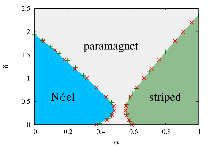
Thus, finally, in Fig. 7 we show our best estimate for the $T=0$ phase diagram of the model in the $\alpha\delta$ plane. For reasons given above the phase boundaries are determined from LSUB$\infty(1)$ points at which the magnetic order parameter $M$ vanishes. These points are determined from extrapolating our LSUB$n$ results for both quasiclassical AFM phases with Eq. (23), and using the data sets with $n=\{2,6,10\}$, which overcome any errors associated with the $(4m-2)/4m$ staggering effects discussed above, as input. Points on the two (i.e., Néel and striped) phase boundaries are shown both at fixed values of $\alpha$ and fixed values of $\delta$. The former [indicated by green plus $(+)$ symbols] are obtained from curves such as those shown in Fig. 4. They thereby represent the corresponding points $\delta_{c_{1}}^{>}(\alpha)$ [and also $\delta_{c_{1}}^{<}(\alpha)$ for fixed $\alpha$ in the range $\alpha_{c_{1}}(0)<\alpha<\alpha_{1}^{>}$] for the Néel phase, and $\delta_{c_{2}}^{>}(\alpha)$ [and also $\delta_{c_{2}}^{<}(\alpha)$ for fixed $\alpha$ in the range $\alpha_{2}^{<}<\alpha<\alpha_{c_{2}}(0)$] for the striped phase. The latter [indicated by red cross $(\times)$ symbols] are similarly obtained from corresponding extrapolated curves for $M$ as a function of $\alpha$ for various fixed values of $\delta$. They are hence the respective points $\alpha_{c_{1}}(\delta)$ for the Néel phase and $\alpha_{c_{2}}(\delta)$ for the striped phase.

One can clearly see from Fig. 7 that on both phase boundaries the two sets of critical points, obtained from the completely independent results at fixed values of $\alpha$ and fixed values of $\delta$, agree extremely well with one another. This is definite evidence for both the consistency and high accuracy of the extrapolation procedure that we have adopted.

Perhaps the most striking aspect of the $T=0$ phase diagram is the marked “avoided crossing” behavior of the two reentrant phase boundaries. We note that the major portions of the upper parts of both boundaries (i.e., for $0\leq\alpha\lesssim 0.4$ for the Néel case and $\alpha\gtrsim 0.6$ for the striped case) are quite well approximated as straight lines. Thus, if these (approximate) straight lines were then to be extended they would cross, and the Néel line would intersect the $\delta=0$ axis at a value rather close to the monolayer striped QCP at $\alpha_{c_{2}}(0)$, while the striped line would intersect the $\delta=0$ axis at a value close to the monolayer Néel QCP at $\alpha_{c_{1}}(0)$.

We have studied a frustrated spin-$\frac{1}{2}$ $J_{1}$–$J_{2}$–$J_{3}$–$J_{1}^{\perp}$ Heisenberg antiferromagnet on an $AA$-stacked honeycomb lattice in the case when $J_{1}>0$, $J_{3}=J_{2}\equiv\alpha J_{1}>0$, and $J_{1}^{\perp}\equiv\delta J_{1}>0$. In particular, we have used the CCM implemented to very high order of approximation to give an accurate description of its $T=0$ quantum phase diagram in the window $0\leq\alpha\leq 1$, $0\leq\delta\leq 1$ of the $\alpha\delta$ plane. This window includes two quasiclassical phases with AFM magnetic order (viz., the Néel and striped phases), plus an intermediate paramagnetic phase that exhibits VBC order of various types.

References

- Sachdev (2011) S. Sachdev, Quantum Phase Transitions, 2nd ed. (Cambridge University Press, Cambridge, UK, 2011).
- Sachdev (2008) S. Sachdev, Nat. Phys. 4, 173 (2008).
- Schmidt and Uhrig (2003) K. P. Schmidt and G. S. Uhrig, Phys. Rev. Lett 90, 227204 (2003).
- Nikuni et al. (2000) T. Nikuni, M. Oshikawa, A. Oosawa, and H. Tanaka, Phys. Rev. Lett. 84, 5868 (2000).
- Cavadini et al. (2001) N. Cavadini, G. Heigold, W. Henggeler, A. Furrer, H.-U. Güdel, K. Krämer, and H. Mutka, Phys. Rev. B 63, 172414 (2001).
- Rüegg et al. (2003) Ch. Rüegg, N. Cavadini, A. Furrer, H.-U. Güdel, K. Krämer, H. Mutka, A. Wildes, K. Habicht, and P. Vorderwisch, Nature 423, 62 (2003).
- Oosawa et al. (2003) A. Oosawa, M. Fujisawa, T. Osakabe, K. Kakurai, and H. Tanaka, J. Phys. Soc. Jpn. 72, 1026 (2003).
- Giamarchi et al. (2008) Th. Giamarchi, Ch. Rüegg, and O. Tchernyshyov, Nat. Phys. 4, 198 (2008).
- Fritz et al. (2011) L. Fritz, R. L. Doretto, S. Wessel, S. Wenzel, S. Burdin, and M. Vojta, Phys. Rev. B 83, 174416 (2011).
- Kageyama et al. (1999) H. Kageyama, K. Yoshimura, R. Stern, N. V. Mushnikov, K. Onizuka, M. Kato, K. Kosuge, C. P. Slichter, T. Goto, and Y. Ueda, Phys. Rev. Lett. 82, 3168 (1999).
- Kodama et al. (2002) K. Kodama, M. Takigawa, M. Horvatić, C. Berthier, H. Kageyama, Y. Ueda, S. Miyahara, F. Becca, and F. Mila, Science 298, 395 (2002).
- Miyahara and Ueda (2003) S. Miyahara and K. Ueda, J. Phys.: Condens. Matter 15, R327– (2003).
- Miyahara and Ueda (1999) S. Miyahara and K. Ueda, Phys. Rev. Lett. 82, 3701 (1999).
- Sriram Shastry and Sutherland (1981) B. Sriram Shastry and B. Sutherland, Physica B+C 108, 1069 (1981).
- Farnell et al. (2014) D. J. J. Farnell, O. Götze, J. Richter, R. F. Bishop, and P. H. Y. Li, Phys. Rev. B 89, 184407 (2014).
- Koga and Kawakami (2000) A. Koga and N. Kawakami, Phys. Rev. Lett. 84, 4461 (2000).
- Corboz and Mila (2013) P. Corboz and F. Mila, Phys. Rev. B 87, 115144 (2013).
- Abendschein and Capponi (2008) A. Abendschein and S. Capponi, Phys. Rev. Lett. 101, 227201 (2008).
- Dorier et al. (2008) J. Dorier, K. P. Schmidt, and F. Mila, Phys. Rev. Lett. 101, 250402 (2008).
- Corboz and Mila (2014) P. Corboz and F. Mila, Phys. Rev. Lett. 112, 147203 (2014).
- Foltin et al. (2014) G. R. Foltin, S. R. Manmana, and K. P. Schmidt, Phys. Rev. B 90, 104404 (2014).
- Laflorencie and Mila (2007) N. Laflorencie and F. Mila, Phys. Rev. Lett. 99, 027202 (2007).
- Schmidt et al. (2008) K. P. Schmidt, J. Dorier, A. M. Läuchli, and F. Mila, Phys. Rev. Lett. 100, 090401 (2008).
- Picon et al. (2008) J.-D. Picon, A. F. Albuquerque, K. P. Schmidt, N. Laflorencie, M. Troyer, and F. Mila, Phys. Rev. B 78, 184418 (2008).
- Chen et al. (2010) P. Chen, C.-Y. Lai, and M.-F. Yang, Phys. Rev. B 81, 020409(R) (2010).
- Albuquerque et al. (2011) A. F. Albuquerque, N. Laflorencie, J.-D. Picon, and F. Mila, Phys. Rev. B 83, 174421 (2011).
- Murakami et al. (2013) Y. Murakami, T. Oka, and H. Aoki, Phys. Rev. B 88, 224404 (2013).
- Sandvik et al. (1995) A. W. Sandvik, A. V. Chubukov, and S. Sachdev, Phys. Rev. B 51, 16483 (1995).
- Chubukov and Morr (1995) A. V. Chubukov and D. K. Morr, Phys. Rev. B 52, 3521 (1995).
- Millis and Monien (1996) A. J. Millis and H. Monien, Phys. Rev. B 54, 16172 (1996).
- Wang et al. (2006) L. Wang, K. S. D. Beach, and A. W. Sandvik, Phys. Rev. B 73, 014431 (2006).
- Ganesh et al. (2011) R. Ganesh, S. V. Isakov, and A. Paramekanti, Phys. Rev. B 84, 214412 (2011).
- Lin and Shen (2000) H.-Q. Lin and J. L. Shen, J. Phys. Soc. Jpn. 69, 878 (2000).
- Alet et al. (2016) F. Alet, K. Damle, and S. Pujari, Phys. Rev. Lett. 117, 197203 (2016).
- Richter et al. (2006) J. Richter, O. Derzhko, and T. Krokhmalskii, Phys. Rev. B 74, 144430 (2006).
- Derzhko et al. (2010) O. Derzhko, T. Krokhmalskii, and J. Richter, Phys. Rev. B 82, 214412 (2010).
- Lee and Sachdev (2014) J. Lee and S. Sachdev, Phys. Rev. B 90, 195427 (2014).
- Oitmaa and Singh (2012) J. Oitmaa and R. R. P. Singh, Phys. Rev. B 85, 014428 (2012).
- Zhang et al. (2014) H. Zhang, M. Arlego, and C. A. Lamas, Phys. Rev. B 89, 024403 (2014).
- Arlego et al. (2014) M. Arlego, C. A. Lamas, and H. Zhang, J. Phys.: Conf. Ser. 568, 042019 (2014).
- Bishop and Li (2017) R. F. Bishop and P. H. Y. Li, Phys. Rev. B 95, 134414 (2017).
- Zhang et al. (2016) H. Zhang, C. A. Lamas, M. Arlego, and W. Brenig, Phys. Rev. B 93, 235150 (2016).
- Gómez Albarracín and Rosales (2016) F. A. Gómez Albarracín and H. D. Rosales, Phys. Rev. B 93, 144413 (2016).
- Krokhmalskii et al. (2017) T. Krokhmalskii, V. Baliha, O. Derzhko, J. Schulenburg, and J. Richter, Phys. Rev. B 95, 094419 (2017).
- Smirnova et al. (2009) O. Smirnova, M. Azuma, N. Kumada, Y. Kusano, M. Matsuda, Y. Shimakawa, T. Takei, Y. Yonesaki, and N. Kinomura, J. Am. Chem. Soc. 131, 8313 (2009).
- Okubo et al. (2010) S. Okubo, F. Elmasry, W. Zhang, M. Fujisawa, T. Sakurai, H. Ohta, M. Azuma, O. A. Sumirnova, and N. Kumada, J. Phys.: Conf. Ser. 200, 022042 (2010).
- Bloch et al. (2008) I. Bloch, J. Dalibard, and W. Zwerger, Rev. Mod. Phys. 80, 885 (2008).
- Duan et al. (2003) L.-M. Duan, E. Demler, and M. D. Lukin, Phys. Rev. Lett. 91, 090402 (2003).
- Tao et al. (2014) H.-S. Tao, Y.-H. Chen, H.-F. Lin, H.-D. Liu, and W.-M. Liu, Sci. Rep. 4, 5367 (2014).
- Dey and Sensarma (2016) S. Dey and R. Sensarma, Phys. Rev. B 94, 235107 (2016).
- Rastelli et al. (1979) E. Rastelli, A. Tassi, and L. Reatto, Physica B & C 97, 1 (1979).
- Fouet et al. (2001) J. B. Fouet, P. Sindzingre, and C. Lhuillier, Eur. Phys. J. B 20, 241 (2001).
- Cabra et al. (2011) D. C. Cabra, C. A. Lamas, and H. D. Rosales, Phys. Rev. B 83, 094506 (2011).
- Farnell et al. (2011) D. J. J. Farnell, R. F. Bishop, P. H. Y. Li, J. Richter, and C. E. Campbell, Phys. Rev. B 84, 012403 (2011).
- Bishop and Li (2012) R. F. Bishop and P. H. Y. Li, Phys. Rev. B 85, 155135 (2012).
- Li et al. (2012a) P. H. Y. Li, R. F. Bishop, D. J. J. Farnell, and C. E. Campbell, Phys. Rev. B 86, 144404 (2012a).
- Senthil et al. (2004a) T. Senthil, A. Vishwanath, L. Balents, S. Sachdev, and M. P. A. Fisher, Science 303, 1490 (2004a).
- Senthil et al. (2004b) T. Senthil, L. Balents, S. Sachdev, A. Vishwanath, and M. P. A. Fisher, Phys. Rev. B 70, 144407 (2004b).
- Kümmel et al. (1978) H. Kümmel, K. H. Lührmann, and J. G. Zabolitzky, Phys Rep. 36C, 1 (1978).
- Bishop and Lührmann (1978) R. F. Bishop and K. H. Lührmann, Phys. Rev. B 17, 3757 (1978).
- Bishop and Lührmann (1982) R. F. Bishop and K. H. Lührmann, Phys. Rev. B 26, 5523 (1982).
- Arponen (1983) J. Arponen, Ann. Phys. (N.Y.) 151, 311 (1983).
- Bishop and Kümmel (1987) R. F. Bishop and H. G. Kümmel, Phys. Today 40(3), 52 (1987).
- Arponen et al. (1987) J. S. Arponen, R. F. Bishop, and E. Pajanne, Phys. Rev. A 36, 2519 (1987).
- Bartlett (1989) R. J. Bartlett, J. Phys. Chem. 93, 1697 (1989).
- Arponen and Bishop (1991) J. S. Arponen and R. F. Bishop, Ann. Phys. (N.Y.) 207, 171 (1991).
- Bishop (1991) R. F. Bishop, Theor. Chim. Acta 80, 95 (1991).
- Bishop (1998) R. F. Bishop, in Microscopic Quantum Many-Body Theories and Their Applications, Lecture Notes in Physics Vol. 510, edited by J. Navarro and A. Polls (Springer-Verlag, Berlin, 1998) pp. 1–70.
- Zeng et al. (1998) C. Zeng, D. J. J. Farnell, and R. F. Bishop, J. Stat. Phys. 90, 327 (1998).
- Farnell and Bishop (2004) D. J. J. Farnell and R. F. Bishop, in Quantum Magnetism, Lecture Notes in Physics Vol. 645, edited by U. Schollwöck, J. Richter, D. J. J. Farnell, and R. F. Bishop (Springer-Verlag, Berlin, 2004) pp. 307–348.
- Bishop et al. (1994) R. F. Bishop, R. G. Hale, and Y. Xian, Phys. Rev. Lett. 73, 3157 (1994).
- Zeng et al. (1995) C. Zeng, I. Staples, and R. F. Bishop, J. Phys.: Condens. Matter 7, 9021 (1995).
- Zeng et al. (1996) C. Zeng, I. Staples, and R. F. Bishop, Phys. Rev. B 53, 9168 (1996).
- Bishop et al. (2000) R. F. Bishop, D. J. J. Farnell, S. E. Krüger, J. B. Parkinson, J. Richter, and C. Zeng, J. Phys.: Condens. Matter 12, 6887 (2000).
- Krüger et al. (2000) S. E. Krüger, J. Richter, J. Schulenburg, D. J. J. Farnell, and R. F. Bishop, Phys. Rev. B 61, 14607 (2000).
- Farnell et al. (2001) D. J. J. Farnell, K. A. Gernoth, and R. F. Bishop, Phys. Rev. B 64, 172409 (2001).
- Darradi et al. (2005) R. Darradi, J. Richter, and D. J. J. Farnell, Phys. Rev. B 72, 104425 (2005).
- Bishop et al. (2008a) R. F. Bishop, P. H. Y. Li, R. Darradi, and J. Richter, EPL 83, 47004 (2008a).
- Bishop et al. (2008b) R. F. Bishop, P. H. Y. Li, R. Darradi, J. Richter, and C. E. Campbell, J. Phys.: Condens. Matter 20, 415213 (2008b).
- Bishop et al. (2009) R. F. Bishop, P. H. Y. Li, D. J. J. Farnell, and C. E. Campbell, Phys. Rev. B 79, 174405 (2009).
- Bishop et al. (2010a) R. F. Bishop, P. H. Y. Li, D. J. J. Farnell, and C. E. Campbell, Phys. Rev. B 82, 024416 (2010a).
- Bishop et al. (2010b) R. F. Bishop, P. H. Y. Li, D. J. J. Farnell, and C. E. Campbell, Phys. Rev. B 82, 104406 (2010b).
- Bishop and Li (2011) R. F. Bishop and P. H. Y. Li, Eur. Phys. J. B 81, 37 (2011).
- Li and Bishop (2012) P. H. Y. Li and R. F. Bishop, Eur. Phys. J. B 85, 25 (2012).
- Li et al. (2012b) P. H. Y. Li, R. F. Bishop, D. J. J. Farnell, J. Richter, and C. E. Campbell, Phys. Rev. B 85, 085115 (2012b).
- Li et al. (2012c) P. H. Y. Li, R. F. Bishop, C. E. Campbell, D. J. J. Farnell, O. Götze, and J. Richter, Phys. Rev. B 86, 214403 (2012c).
- Bishop et al. (2012) R. F. Bishop, P. H. Y. Li, D. J. J. Farnell, and C. E. Campbell, J. Phys.: Condens. Matter 24, 236002 (2012).
- Bishop et al. (2013) R. F. Bishop, P. H. Y. Li, and C. E. Campbell, J. Phys.: Condens. Matter 25, 306002 (2013).
- Richter et al. (2015) J. Richter, R. Zinke, and D. J. J. Farnell, Eur. Phys. J. B 88, 2 (2015).
- Bishop and Li (2015) R. F. Bishop and P. H. Y. Li, EPL 112, 67002 (2015).
- Bishop et al. (2015) R. F. Bishop, P. H. Y. Li, O. Götze, J. Richter, and C. E. Campbell, Phys. Rev. B 92, 224434 (2015).
- Bishop and Li (2016) R. F. Bishop and P. H. Y. Li, J. Magn. Magn. Mater. 407, 348 (2016).
- Li et al. (2016) P. H. Y. Li, R. F. Bishop, and C. E. Campbell, J. Phys.: Conf. Ser. 702, 012001 (2016).
- Li and Bishop (2016) P. H. Y. Li and R. F. Bishop, Phys. Rev. B 93, 214438 (2016).
- Li and Bishop (2018) P. H. Y. Li and R. F. Bishop, J. Magn. Magn. Mater. 449, 127 (2018).
- (96) We use the program package CCCM of D. J. J. Farnell and J. Schulenburg, see http://www-e.uni-magdeburg.de/jschulen/ccm/index.html.
- Löw (2009) U. Löw, Condensed Matter Physics 12, 497 (2009).
- Jiang (2012) F. J. Jiang, Eur. Phys. J. B 85, 402 (2012).