A high-sensitivity polarimeter using a ferro-electric liquid crystal modulator
Abstract
We describe the HIgh Precision Polarimetric Instrument (HIPPI), a polarimeter built at UNSW Australia and used on the Anglo-Australian Telescope (AAT). HIPPI is an aperture polarimeter using a ferro-electric liquid crystal modulator. HIPPI measures the linear polarization of starlight with a sensitivity in fractional polarization of 4 10-6 on low polarization objects and a precision of better than 0.01% on highly polarized stars. The detectors have a high dynamic range allowing observations of the brightest stars in the sky as well as much fainter objects. The telescope polarization of the AAT is found to be 48 5 10-6 in the g′ band.
keywords:
polarization – instrumentation: polarimeters – techniques: polarimetric.1 Introduction
Stellar polarization can be measured to very high sensitivity with ground-based telescopes. Unlike photometry where atmospheric effects limit the achievable precision, polarimetry is a differential measurement and so there is no fundamental limit on the sensitivity. Kemp et al. (1987) measured the polarization of the Sun to levels of parts in ten million, and astronomical polarimeters have been built that measure stellar polarization at the parts per million level (Hough et al., 2006; Wiktorowicz & Matthews, 2008). Interest in such instruments has been driven, in particular, by the possibility of detecting polarized scattered light from hot Jupiter type exoplanets, which is predicted to be at levels of or less in the combined light of the star and the planet (Seager, Whitney & Sasselov, 2000; Lucas et al., 2009). Such instruments also have other applications such as the study of the local interstellar medium (Bailey, Lucas & Hough, 2010; Frisch et al., 2012) and the scattered light from debris disks (Wiktorowicz et al., 2010).
The standard method used for most high sensitivity polarization studies has been the use of the photoelastic modulator (PEM) technology pioneered by James Kemp (Kemp, 1969; Kemp & Barbour, 1981; Kemp et al., 1987). These devices modulate polarization at frequencies of 20 – 100 kHz by means of the stress birefringence in an optical material made to vibrate at its natural frequency using piezoelectric transducers. While PEMs have proved very successful in this role they nevertheless have a number of disadvantages. While a high modulation frequency is desirable to minimize the effects of variations due to seeing and tracking errors, the frequency of PEMs is higher than is really needed for this purpose. The high frequency can present problems in providing a suitable detector system. Many detector types can either not operate at the required speed, or can only do so with some compromise in their noise performance. PEMs are inherently sine-wave modulators and thus the efficiency of a PEM polarimeter is less than that of an ideal square wave modulator by a factor of at least (actually slightly more than this, see Hough et al. 2006). PEMs are also quite bulky and thus difficult to use where space is limited.
In this paper we describe a high-sensitivity polarimeter using an alternate type of polarization modulator, a ferro-electric liquid crystal modulator (FLC). FLCs are electrically switchable wave plates consisting of a thin layer of liquid crystal material sandwiched between two glass plates. They have a fixed retardation and the orientation of the optical axis can be controlled by an applied drive voltage. FLCs have been used, in particular, for solar polarimetry (e.g. Gandorfer, 1999; Martínez Pillet et al., 1999; Hanaoka, 2004) and also for the Extreme Polarimeter (ExPo Rodenhuis et al., 2012), a high contrast imaging polarimeter and the SPHERE/ZIMPOL instrument for the ESO VLT (Bazzon et al., 2012; Roelfsema et al., 2014).
Our polarimeter HIPPI (HIgh Precision Polarimetric Instrument) has been used on the 3.9m Anglo-Australian Telescope (AAT) at Siding Spring Observatory for two observing runs during 2014. The design of HIPPI has been based on that of the previous PlanetPol instrument (Hough et al., 2006). However, HIPPI differs from PlanetPol in being optimised for observation at blue wavelengths. This is based on results such as those of Pont et al. (2013) and Evans et al. (2013) that indicate the presence of strong Rayleigh scattering at blue wavelengths from the exoplanet HD 189733b making these wavelengths the most suitable for detecting exoplanet polarization.
2 Instrument Description
2.1 Overview
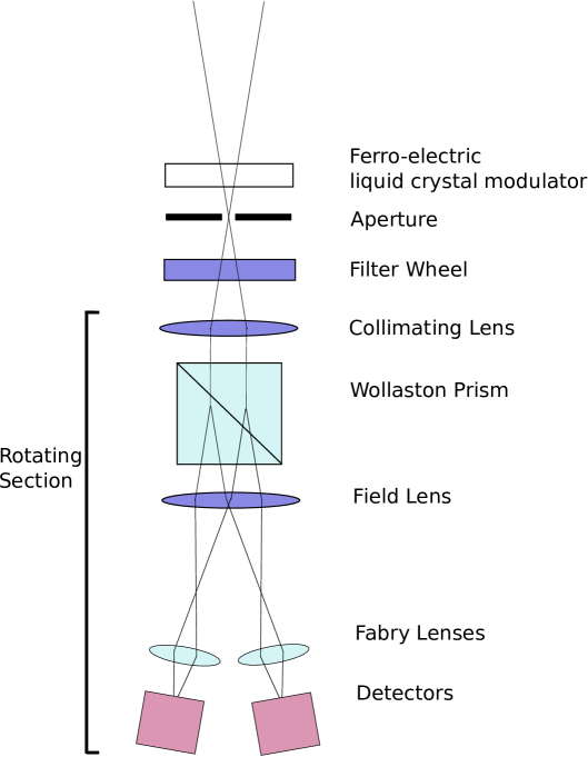
A schematic diagram of the HIPPI optical system is given in figure 1. The FLC modulator is the first element in the optical system. This is an important design feature since any optics placed ahead of the modulator could potentially induce spurious polarization effects, for example, polarization due to inclined mirrors or residual stress birefringence in refracting elements. Following the FLC is an aperture of 1 mm diameter corresponding to 6.7 arc seconds at the AAT f/8 focus. This is followed by a six position filter wheel.
The filters used with HIPPI have been Sloan Digital Sky Survey (SDSS, Fukugita et al., 1996) g′ and r′ filters (from Omega Optical, giving wavelength ranges of 400 – 550 nm and 550 – 700 nm respectively). There is also a short pass filter which passes wavelengths shorter than 500 nm (referred to as 500SP). The instrument has little throughput below about 350 nm due to absoprtion in the calcite prism so the range of this filter is from 350 – 500 nm. The filter wheel also includes a clear position and a blank setting that can be used for taking dark measurements.
The polarization analyser is a calcite Wollaston prism that provides a 20 degree beam separation. This is placed between two lenses to collimate the light through the prism. A Fabry lens in each beam images the telescope pupil onto the two detectors. The whole optical system from the collimating lens to the detectors is rotatable about the optical axis using a Thorlabs NR360S NanoRotator stage. Rotating this system through 90 degrees relative to the modulator has the effect of reversing the sign of the modulation seen by the detectors and provides a “second stage chopping” which helps to improve accuracy by eliminating some systematic effects (Kemp & Barbour, 1981). A similar system was used in PlanetPol (Hough et al., 2006). All the optics are anti-reflection coated for the wavelength range 350 – 700 nm.
The instrument components are mounted on a standard 300 mm square aluminium optical breadboard that is attached by 90 degree brackets to a mounting plate that bolts to the back of the telescope. Many of the structural components, optical mounts and electronics enclosures have been constructed by 3D printing in ABS plastic. The instrument is therefore compact and lightweight (10 kg).
2.2 Ferro-electric liquid crystal modulators
Two different FLC modulators have been used with HIPPI. The first is a LV1300-AR-OEM device from Micron Technology111This company no longer supplies such devices. It is designed for the 400–700 nm range and is 12.7 mm in diameter housed in a 25 mm diameter cell. The second is an MS Series polarization rotator from Boulder Nonlinear Systems (BNS) designed for the wavelength range 425 – 675 nm and is 22 mm in diameter with a 15 mm useful aperture. Both devices are designed to be half-wave retarders at a wavelength near 500 nm, and depart from half-wave away from this wavelength as discussed further in section 3.6.
The two modulators are very similar in their operation and provide good polarization modulation with a 5 V drive waveform. However, we have found the BNS modulator to produce much lower levels of instrumental polarization, and it is therefore currently the preferred option.
Electrically the modulators are equivalent to capacitors of 200 nF and therefore require a drive circuit capable of driving at high speed into a capacitive load. The devices can also be damaged by sustained DC voltages. We have desiged and built a drive circuit consisting of a two-pole Butterworth high pass filter followed by an amplifier using a NPN/PNP transistor pair output stage. The filter ensures no DC or low frequency components reach the device. The drive amplifier has the high slew rate, and high drive current needed to drive a square wave into the capacitive load.
The drive waveforms are generated in software. A simple square wave between +5 V and 5 V has been used for all the observations described in this paper. Our system allows selection of modulation frequencies between 200 Hz and 2 kHz. We have found 500 Hz to be a good choice for actual observing, providing a close to square wave modulation, while being fast enough to be insensitive to intensity fluctuations due to seeing or tracking errors.
FLCs are temperature sensitive devices. The switching is faster at higher temperatures and the switching angle is also temperature dependent. To ensure consistent and stable operation we mount the FLC in a temperature controlled lens tube and operate it at a constant temperaure of 25∘ C, maintained to about 0.1∘ C.
2.3 Detectors
The detectors used in HIPPI are compact photomultiplier tube (PMT) modules. The modules contain a metal packaged photomultiplier tube combined with an integrated HT supply. PMTs have substantial advantages of large detector area and low dark noise compared with possible solid-state alternatives such as avalanche photodiodes (as used in PlanetPol) or so-called “silicon photomultipliers”.
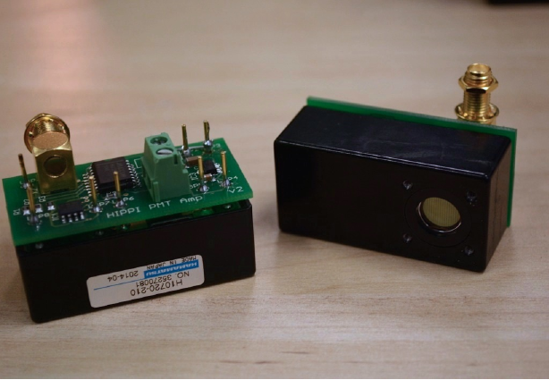
HIPPI uses Hamamatsu H10720-210 PMT modules which have ultra-bialkali photocathodes (Nakamura et al., 2010) providing a quantum efficiency (QE) of 43% at 400 nm. They are compact modules operating off a single 5V supply. For the high photon rates required with HIPPI it is not possible to use the PMT in a photon counting mode. Instead we use a transimpedance amplifier to amplify the photo-current. The amplifiers designed and built for HIPPI use an ultra low noise Texas Instruments OPA 129 operational amplifier with an extremely low input current noise of 0.1 fA Hz-1/2. Remotely switchable transimpedance gains of 105, 106 and 107 V/A can be selected. The PMT module itself provides selectable HT voltages from 500 V to 1100 V corresponding to a variation of the PMT gain from to electrons per photon. The ability to remotely vary both the photomultiplier gain and amplifier gain over a wide range provides a very high dynamic range, allowing HIPPI to observe objects from the brightest stars in the sky to quite faint objects while still providing close to photon noise limited performance.
The PMT amplifiers have been built in surface-mount construction on a compact printed circuit board 25 50 mm that fits on the back of the PMT module as shown in figure 2.
2.4 Instrument Control and Data Acquisition
HIPPI is controlled by software running on a rack mount computer (Intel quad core i7, 8 GB RAM, 2 1 TB disks). The computer runs the Windows 7 Professional operating system and the software has been developed using the National Instruments LabVIEW graphical programming environment.
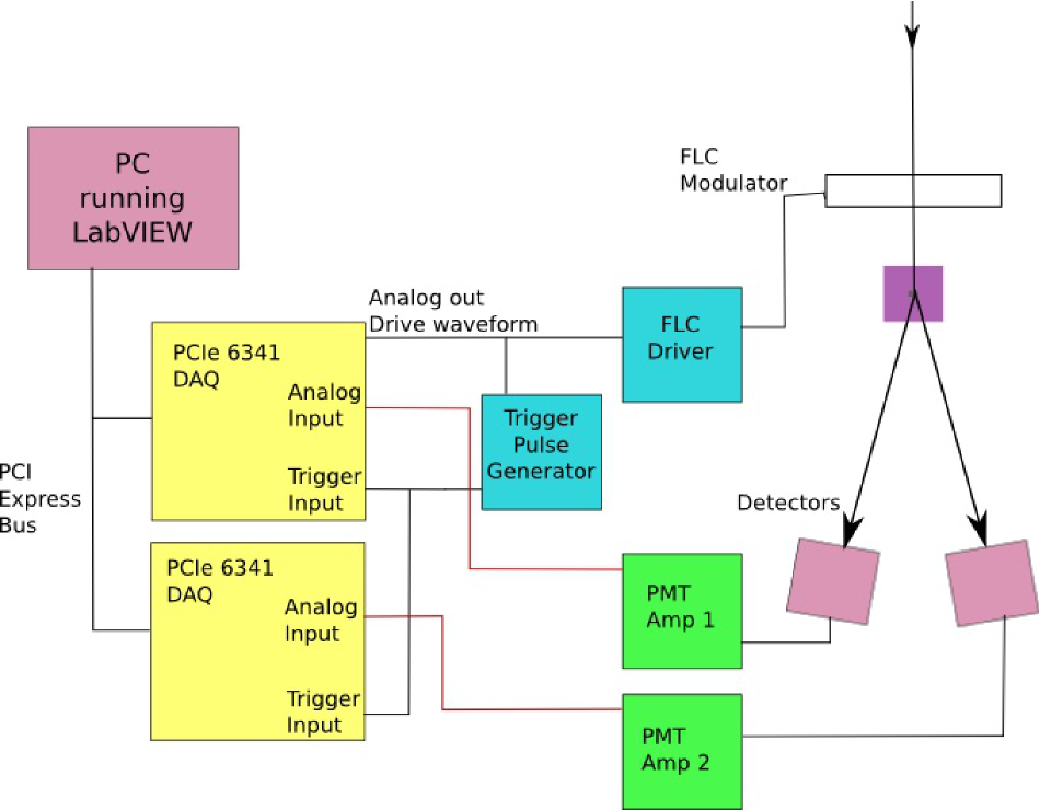
The interface to drive the FLC and read data from the detectors makes use of two National Instruments data acquisition modules (PCIe 6341) each of which provides 16-bit analog input and output channels. The drive waveform for the modulator is generated in software and output from one of the modules. A trigger digital input signal is generated from the rising edge of the square wave and fed to both modules. The detector signals are read by analog input channels on each module. A schematic diagram of the system is shown in figure 3.
The HIPPI software system also provides control of the FLC temperature, the filter wheel selection, the rotation of the Wollaston prism and detector section of the optics, and the gain and HT voltage settings for the detectors.
In operation the analog input channels are sampled at 10 microsecond intervals and read for an integration time of typically 1 second resulting in 100000 data points for each channel. The timing is controlled to start on the trigger input so that the sampling always has the same phase relationship with the modulator waveform. The data are then folded in software over the modulation cycle. For our standard 500 Hz modulation this results in an array of 200 points from each channel.
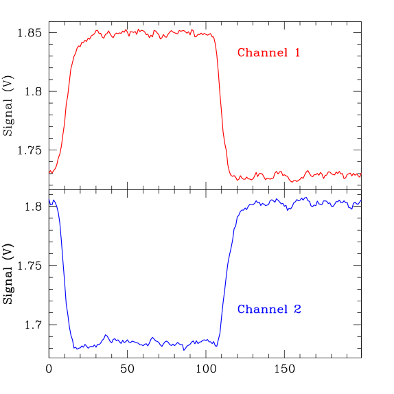
Figure 4 shows what the resulting waveforms look like when a polarized star is being observed. The modulation is of opposite sign in the two channels as they correspond to the two orthogonal polarization states from the Wollaston prism. Zero on the diagram corresponds to the rising edge of the square wave drive signal to the FLC. The delay of about 100 s in the observed signal is a combination of the finite switching time of the FLC, and the time constant (22 s) of the detector amplifiers.
These modulation waveforms are displayed to the user and output to the data files every integration. The amplitude of the modulation is a measure of the polarization of the source. A quick-look data reduction capability is built into the observing software and derives the fractional polarization (p) as follows.
| (1) |
where X is the signal from the first flat part of the waveform (points from about 20 – 100 in figure 4), and Y is the signal from the second flat section (about 120 – 200), with points around the two transitions being ignored. This simple quick-look reduction allows immediate evaluation of incoming data, but excludes some corrections such as subtracting the small bias and dark signals. The offline data reduction described in section 3 uses the full waveform and inlcudes all these corrections.
2.5 Observing Procedure
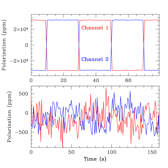
The normal observing procedure with HIPPI is to make a sequence with the Wollaston and detectors rotated to two positions 90 degrees apart (referred to as A and B), in the cycle A, B, B, A with this sequence then being repeated as many times as required. This rotation causes the sign of the modulation in each channel to reverse. It results in the p value obtained for each integration (with Equation 1 above) following the sequence as shown in figure 5.
Note that while the polarization changes are almost symmetric about zero for the highly polarized star in the top panel, a significant offset from zero is apparent in the bottom panel.
An observation of this type measures only one Stokes parameter of linear polarization. To get the orthogonal Stokes parameter the entire instrument is rotated through 45 degrees and the sequence repeated. The rotation is performed using the AAT’s Cassegrain instrument rotator. In practice we also repeat the observations at telescope position angles of 90 and 135 degrees to allow removal of instrumental polarization.
3 Data Reduction
The HIPPI data processing and calibration procedure has at its heart a Mueller matrix model of the instrument. The parameters of the Mueller matrix are varied according to the state of the system. The system parameters vary over a single integration as a result of the varying voltage applied to the FLC.
The Mueller matrix of an optical system (such as HIPPI) relates the output Stokes vector to the input Stokes vector through:
| (2) |
The Mueller matrix for HIPPI is not constant since it changes through the cycle of the modulator. We can describe a full integration using a system matrix . The system matrix is an N by 4 matrix, where each row is a state of the system, corresponding to a single data point in the modulation curve. Multiplying the input Stokes vector by the system matrix gives the vector of observed intensities seen at the detector during the modulation cycle (e.g. the points plotted in figure 4, where ).
| (3) |
It can be seen that the N rows of the system matrix are simply the top rows of the Mueller matrices for HIPPI for each of the N states of the instrument through a modulation cycle. Only the top row is needed because this is the row of the Mueller matrix that determines the intensity of the output light, and only intensity is directly measured at the detector.
The optical components HIPPI is made up of are the FLC and the Wollaston prism. the FLC is a retarder, which has the Mueller matrix:
| (4) |
where , , is the retardance, and the angle to the fast axis of the retarder. For a half wave plate the retardance is radians. FLCs are sometimes modelled as having a linear depolarization component (Gendre et al., 2010), with a Mueller matrix of:
| (5) |
where is the degree of depolarization.
The Wollaston prism behaves as two perpendicular polarizers. A polarizer has a Mueller matrix of:
| (6) |
where , , is the efficiency of the polarizer, and is the angle of the polarizer axis to that defined for the incoming beam. Wollaston prisms are very efficient, and we assume .
The combined Mueller matrix for HIPPI can now be written in terms of these matrices as:
| (7) |
and can be used to derive the system matrix for HIPPI as already described. The N rows of the system matrix are derived from the Mueller matrices for the state of the system at each modulation point where each row differs due to different values of (in ) and (in ).
The other main parameter in the Mueller matrix is the retardance . This does not vary around the modulation cycle, but it is a strong function of wavelength. The retardance is close to half-wave only at a single wavelength. The effect of a retardance that is not exactly half-wave is to reduce the amplitude of the modulation curve by a factor of . Incorporating the full wavelength dependence of retardance in our reduction model would be impracticable as a single observation can cover a wide range of wavelengths. Instead we perform the reduction assuming a half-wave retardance, and then account for the wavelength dependence effects by scaling the polarization with an efficiency correction that can be determined empirically from standard star observations (section 4.3) or can be derived from a model (section 3.6).
| (8) |
where is the pseudo-inverse of , which we calculate numerically using the method of Rust, Burrus & Schneeburger (1966). This gives the source Stokes parameters in terms of the observed modulation data .
In practice, because HIPPI isn’t designed to measure circular polarization, we use only the first three columns of , to obtain a least squares estimate of the components of , ( , and ), in the manner of Gendre, Foulonneau & Bigué (2010) and then divide and by for the normalised Stokes parameters.
3.1 Calibration
To apply equation 8 we need to know how the waveplate angle and the depolarization factor vary thrugh the modulation cycle of the FLC as these are the only varying components that enter into . This is done using a laboratory calibration procedure where we input known polarization states into the instrument using a lamp and a rotatable polarizer. Measurements are made of the full modulation curve with the polarizer stepped through a full rotation in 10 or 20 degree steps. By fitting a Malus law (Hecht, 2001) — modified to include an intensity offset and a phase shift — to the intensity as a function of polarizer angle we determine and for each point in the modulation cycle.
To reduce the effect of noise in the calibration measurements the array of values is smoothed by replacing the last 50 modulation points in the plateau regions (i.e. the last 50 before the FLC is switched) by their average value. Only the last half of the plateau region is used because we have found that the Micron Technology FLC does not have a stable until this point – it is still approaching maximum/minimum.
The values of and are determined separately for each of the two PMT channels. This is to allow for timing differences between the two channels. The depolarization () is included primarily to account for the switching part of the modulation cycle, where the switching can occur faster than the detector response resulting in a reduction in apparent polarization. The results are normalized such that it does not result in any scaling of the measured polarization, and therefore does not attempt to duplicate the wavelength dependent efficiency correction.
3.2 Measurements
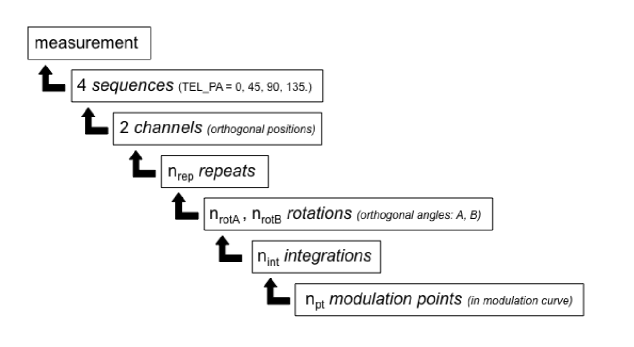
For a given filter and target, a measurement involves taking data at 4 position angles of the Cassegrain rotator corresponding to 0, 45, 90 and 135 degrees. In general, a sky measurement is also made at each telescope position angle. For very bright targets or high polarization standards or bright targets in moonless conditions a dark measurement may be substituted for the sky measurements. Each sequence is made up of a number of identical repeats each of which consist of a subsequence of a number of rotations; for each rotator position there are a number of integrations, each of which consists of the individual modulation points that make up the modulation curve. The rotation subsequence is typically an ABBA sequence with A and B corresponding to orthogonal rotator positions as described in section 2.5. Figure 6 summarises the components of a measurement.
As an example, a typical bright star measurement with HIPPI consists of sequences at 4 position angles each consisting of 2 repeats (), in an ABBA rotation subsequence (), each consisting of 10 1 second integrations () of a modulation curve consisting of 200 modulation points (). Measurements requiring higher precision have higher numbers of integrations and repeats.
3.3 Statistical treatment of values and errors
The Mueller matrix model of the modulation curve is used to calculate a Q/I and U/I for each integration. However, the co-ordinate frame of the instrument is chosen to match the calibrated rotator positions (see section 4.1, which means that the majority of the modulation points in the curve measure predominantly either Q or U; the other Stokes parameter determination is discarded because it contributes greater noise. The “off-axis” Stokes parameter is measured by significantly fewer modulation points, and is contaminated by the intrinsic FLC polarization. This gives a single Stokes parameter determination for each integration.
The average of all the integrations for a given rotator position is then calculated, and the error calculated from the standard deviation of the points. The average polarization over each rotation, repeat and channel in the sequence is calculated, and the error on this calculated by averaging the statistical errors for each individual rotator position and divding by the square root of the number of these that have been combined. This gives a normalised Stokes parameter measurement for each telescope position angle (), each with an associated error ().
The value of , in the chosen co-ordinate system of the instrument, is obtained from the average of the 0 and 90 degree sequences and the value of from the average of the 45 and 135 degree sequences.
| (9) |
| (10) |
With errors calculated as:
| (11) |
| (12) |
3.4 Sky and dark correction
Sky measurements are made to take account, predominantly, of polarization caused by reflected light from the Moon. The sky sequences are always made with the same HT voltage, gain, telescope position angle and filter as the science sequences. Because the sky signal level is much lower than that from the star, much shorter total integration times can be used for the sky measurements without intoducing significant additional noise. The average modulation curves for the sky data are determined for each PMT channel and rotator position. These are then subtracted from the each of the corrsesponding modulation curves in the science sequence prior to the analysis described in sections 3.2 and 3.3.
In cases where the sky contribution is negligible, for example when observing a bright star in moonless conditions, a dark observation can be used as an alternative to a sky. This is made by using a blank in the filter wheel to exclude any light input to the instrument.
| Spectral Type | Effective Wavelength (nm) | Modulation Efficiency (%) | ||||
|---|---|---|---|---|---|---|
| 500SP | g′ | r′ | 500SP | g′ | r′ | |
| B0 V | 433.2 | 472.6 | 600.8 | 74.3 | 90.8 | 84.4 |
| A0 V | 443.7 | 475.6 | 601.9 | 81.6 | 91.5 | 84.2 |
| F0 V | 447.1 | 479.5 | 603.7 | 83.0 | 92.3 | 83.8 |
| G0 V | 451.2 | 483.4 | 605.5 | 84.6 | 93.0 | 83.5 |
| K0 V | 456.4 | 486.4 | 606.6 | 87.1 | 93.7 | 83.3 |
| M0 V | 459.2 | 490.1 | 610.5 | 88.8 | 93.8 | 82.6 |
| M5 V | 458.1 | 490.0 | 611.4 | 88.3 | 93.7 | 82.4 |
3.5 Coordinate transformation and efficiency calibration
The co-ordinate transformation from the frame of the instrument to that of the sky is carried out by reference to known polarization standards. Polarization angle is calculated by:
| (13) |
The difference between the calculated angle with that known for the standards becomes the angular correction, and all other measurements are rotated by this value.
The linear polarization, P, is given by:
| (14) |
This polarization then needs to be scaled by multiplying by an efficiency correction to account for the wavelength dependence of the retardance of the modulator. This efficiency correction can either be determined empirically using polarized standard stars as described in section 4.3, or determined using the bandpass model described in section 3.6.
3.6 Filters and bandpass model
The filters used in HIPPI are relatively broad (150 nm for the g′ and r′ filters) and hence the precise effective wavelength will vary with star colour and other factors, and this will, in turn, affect the modulation efficiency which is also a function of wavelength since the modulator is not an achromatic device. To account for these effects we use a bandpass model similar to that described by Hough et al. (2006).
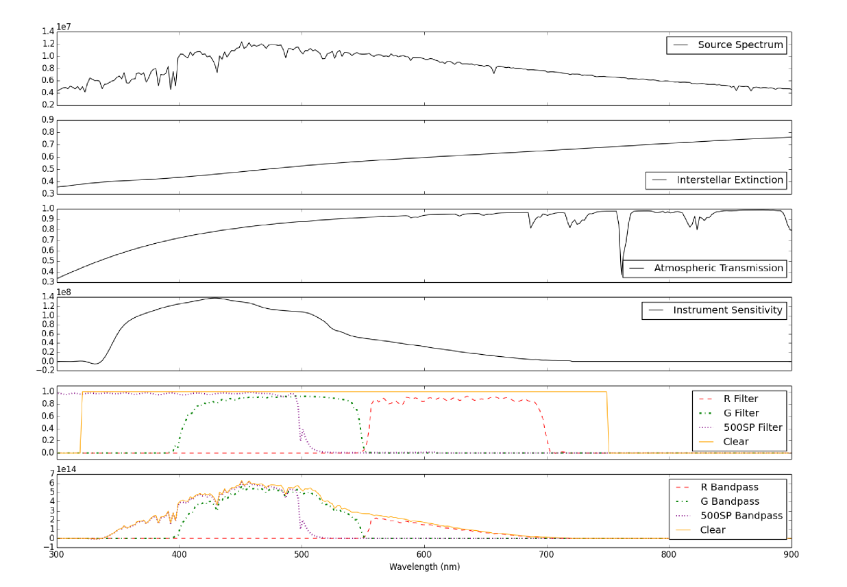
As a starting point for such a model we typically use one of the Castelli & Kurucz (2004) stellar atmosphere models. The spectral energy distribution (SED) given by the model can then be modified for interstellar extinction using the empirical model of Cardelli, Clayton & Mathis (1989). We then correct the SED for its passage through the Earth’s atmosphere by applying an atmospheric transmission correction calculated using the VSTAR modelling code (Bailey & Kedziora-Chudczer, 2012) and including molecular absorption and Rayleigh scattering.
Finally this can be combined with a model of the instrument response which includes the transmission functions of the filters, and the cathode radiant sensitivity (in mA/W) of the PMT as taken from the Hamamatsu data sheet. The final result, which we call is the relative contribution to the output detector signal as a function of wavelength.
The effective wavelength of the observation can be determined from
| (15) |
where the integral is taken over all wavelengths for which is non-zero.
The polarization modulation efficiency correction will be given by
| (16) |
where is the wavelength dependence of the modulation efficiency. For an FLC the efficiency as a function of wavelength is primarily determined by the variation of the retardance with wavelength. According to Gisler, Feller & Gandorfer (2003) the optical path difference () of an FLC can be represented by:
| (17) |
where is the half-wave wavelength, is a parameter describing the dispersion in birefringence of the FLC material, and is the thickness of the FLC layer. In practice can be treated as a single parameter. We have determined these parameters for our two modulators by fitting this formula to a set of laboratory measurements of a polarized source made with HIPPI using a set of narrow band filters. The results are given in table 2.
| Modulator | Micron | BNS |
|---|---|---|
| 505 5 nm | 498 5 nm | |
| nm3 | nm3 |
The properties of the two modulators are very similar, and the value we obtain is almost the same as that found by Gisler et al. (2003) for a similar device.
The modulation efficiency is then given by:
| (18) |
where is the peak efficiency measured at wavelength . Ideally should equal 1, but we find a value of 0.98 is the maximum achievable using laboratory measurement with HIPPI.
Table 1 shows how the effective wavelength and polarization efficiency vary with spectral type. The bandpass model is illustated in figure 7.
4 Performance and Results
The performance of HIPPI has been evaluated based on our observing runs on the AAT over May 8 – 12 2014 and Aug 28 – Sep 2 2014.
4.1 Instrumental polarization
We have found that the FLC modulators used in HIPPI introduce a large instrumental polarization effect which appears to be an intrinsic property of the modulator. Such polarization is thought to arise from multiple internal reflections in the birefringent material between the plates resulting in wavelength dependent fringe patterns in transmittance that are different for light polarized parallel or perpendicular to the fast axis (Gisler et al., 2003; de Juan Ovelar et al., 2012). This effect was found to be present with both our modulators but is a factor of about 3 higher for the Micron Technology modulator (used for the May 8 – 12 observing run) than for the BNS modulator (used for the Aug 28 – Sep 2 run). Even in the BNS case the effect is at the 1000 ppm level and highly variable with wavelength. Since it is due to the modulator that does not rotate, it cannot be removed by our second-stage chopping procedure described earlier.
Fortunately because the instrument only measures one Stokes parameter at a time it is possible to arrange things such that the instrumental polarization is orthogonal to the Stokes parameter being measured. This is done by choosing optimal values for the pair of 90 degree separated angles that are used for rotating the Wollaston prism and detectors. When this is done the instrumental polarization is greatly reduced but it cannot be removed completely. Due to effects such as its wavelength dependence in angle, residual instrumental effects at around the 50 ppm level remain.
The residual instrumental polarization is removed by the procedure of observing at four position angles of the instrument rotator (0, 45, 90, 135) as described in sections 2.5 and 3.2. The 90 degree rotation between the 0, 90 and 45, 135 pairs reverses the sign of the instrumental polarization relative to that from the star, enabling it to removed.
4.2 Telescope polarization
| Star | Date | Filter | P (ppm) | (deg) |
|---|---|---|---|---|
| BS 5854 | Aug 28 | g’ | 35 5 | 113 6 |
| Aug 29 | g′ | 46 4 | 115 17 | |
| Aug 30 | g′ | 50 4 | 114 4 | |
| Sep 2 | g′ | 45 5 | 110 6 | |
| Average | g′ | 44 2 | 114 3 | |
| Beta Hyi | Aug 28 | g′ | 52 3 | 113 4 |
| Aug 29 | g′ | 62 3 | 106 3 | |
| Aug 30 | g′ | 58 3 | 109 4 | |
| Aug 31 | g′ | 52 3 | 106 4 | |
| Average | g′ | 56 2 | 109 2 | |
| Sirius | Aug 31 | g′ | 55 1 | 112 1 |
| Sep 2 | g′ | 48 4 | 108 5 | |
| Average | g′ | 51 2 | 110 3 | |
| Adopted TP | g′ | 48 5 | 111 2 |
The telescope optics can be expected to introduce a small telescope polarization (TP) that must be corrected for. In the case of PlanetPol on the William Herschel Telescope TP was found to be around 15 ppm (Hough et al., 2006). A much larger TP of 250 ppm was found using POLISH on the 5-m Hale Telescope (Wiktorowicz & Matthews, 2008).
| Star | Spectral Type | K | Expected (%) | Refs | |||||||
|---|---|---|---|---|---|---|---|---|---|---|---|
| g′ | r′ | 500SP | |||||||||
| HD 23512 | A0 V | 0.34 | 3.2 | 2.29 | 0.60 | 1.06 | 29.9 | 2.15 | 1, 2 | ||
| HD 147084 | A4 II/III | 0.72 | 3.9 | 4.34 | 0.67 | 1.15 | 32.0 | 3.77 | 4.26 | 3.60 | 3, 4 |
| HD 187929 | F6-G0 I | 0.18 | 3.1 | 1.76 | 0.56 | 1.15 | 93.8 | 1.70 | 1.66 | 5 | |
| Star | Date | Filter | Measured | Expected | Efficiency | Efficiency | ||
|---|---|---|---|---|---|---|---|---|
| (ppm) | (deg) | (ppm) | (deg) | (Observed) | (Modelled) | |||
| HD 23512 | Aug 28 | g′ | 18852 37 | 30.5 0.1 | 21469 | 29.9 | 87.8 | 90.0 |
| HD 147084 | Aug 29 | g′ | 33919 11 | 32.0 0.1 | 37664 | 32.0 | 90.1 | 91.0 |
| Aug 30 | g′ | 33972 12 | 32.0 0.1 | 37665 | 32.0 | 90.2 | 91.0 | |
| Aug 30 | r′ | 34910 17 | 32.1 0.1 | 42619 | 32.0 | 81.9 | 84.2 | |
| Aug 30 | 500SP | 29349 17 | 32.0 0.1 | 35958 | 32.0 | 81.6 | 80.7 | |
| Aug 31 | 500SP | 29337 12 | 31.9 0.1 | 35956 | 32.0 | 81.6 | 80.7 | |
| HD 187929 | Aug 28 | g′ | 15450 9 | 93.5 0.1 | 16950 | 93.8 | 91.1 | 91.2 |
| Aug 29 | g′ | 15493 9 | 93.6 0.1 | 16960 | 93.8 | 91.3 | 91.4 | |
| Sep 2 | g′ | 15560 13 | 93.6 0.1 | 16944 | 93.8 | 91.8 | 91.1 | |
| Sep 2 | 500SP | 14213 16 | 93.8 0.1 | 16570 | 93.8 | 85.7 | 84.7 | |
As the AAT is an equatorially mounted telescope it is not possible to separate the telescope and star polarization in the way described by Hough et al. (2006) making use of the field rotation in an altazimuth mounted telescope.
Instead, we have adopted as our preliminary estimate of the telescope polarization the average of our observations of three stars which we have reason to believe should have very low polarization. One of these is BS 5854 which is one of the low polarization standard stars observed with PlanetPol. It is at a distance of 22.5 pc and had measured polarizations with PlanetPol of 5 ppm or lower (Hough et al., 2006; Bailey et al., 2008). The other two are nearby bright stars Beta Hydri (HIP 2021, BS 98) which is a 2.8 magnitude star at a distance of 7.5 pc, and Sirius ( CMa) at a distance of 2.6 pc. Based on the polarization with distance results of Bailey, Lucas & Hough (2010) these should be expected to have very low polarizations.
The results are given in table 3 for the telescope polarization measurements in the SDSS g′ filter. From smaller numbers of observations we have determined TP = 53 2 ppm, = 110 2 degrees in the 500SP filter, TP = 45 3, ppm = 125 5 degrees in the SDSS r′ filter, and TP = 49 2 ppm, = 117 2 degrees with no filter (the full wavelength range of the detector). These results suggest an increasing TP and a rotation in angle from red to blue.
4.3 Polarized Standard Stars
Observations were made of a number of polarized standard stars. The stars observed are listed in table 4, together with the parameters needed for the bandpass model.
The wavelength dependence of interstellar polarization can be represented by the empirical model (Serkowski, Mathewson & Ford, 1975; Wilking et al., 1980)
| (19) |
where the values of , and are empirical parameters that are fitted to observed wavelength dependent polarization measurements and are given in table 4 for our standard stars.
The expected polarization in any of the HIPPI filters can then be predicted by averaging this function over the bandpass model as described in section 3.6 as follows:
| (20) |
Observations of polarized standard stars are listed in table 5.
It can be seen from table 5 that the repeatability of these measurements from night to night is excellent with polarization agreeing to 0.01 % (100 ppm) or better and the position angles agreeing to typically 0.1 deg. The position angles also agree quite well with the expected values. While the position angle zero point was calibrated using these stars, the agreement between the three stars is an indicator of the accuracy of these measurements. The absolute calibration of position angle is somewhat poorer than the internal errors of 0.1 degree, because it is limited by the available data on standard stars.
Comparing with the predicted values of polarization from table 4 we find that the observed modulation efficiency averages 90 % in the g’ band with somewhat lower values in the 500SP and r’ filters. These can be compared with the predicted efficiencies from the model described in section 3.6 which are given in the final column of the table. It can be seen that the observed efficiencies are in good agreement with the efficiencies predicted by our model. In most cases the measured and observed values agree within 1%, with the largest deviation being 2.3 %. Given that the quoted accuracies of the standard star values are typically around 1% of the measured value this is excellent agreement.
4.4 Polarization Sensitivity
The polarization sensitivity of a polarimeter is its ability to measure small polarization levels, and is equivalent to the precision of measurement on low polarization objects. It can be estimated by looking at the night to night scatter of repeat observations of low polarization stars. In table 6 we show such results for four sets of observations on three stars that have been measured on three or more nights. The data presented here are the instrumental Stokes parameters as measured by HIPPI before corrections for telescope polarization, and position angle zero point.
| Star | Canopus (g′) | Beta Hyi (g′) | BS 5854 (g′) | Beta Hyi (500SP) | ||||
|---|---|---|---|---|---|---|---|---|
| Q/I (ppm) | U/I (ppm) | Q/I (ppm) | U/I (ppm) | Q/I (ppm) | U/I (ppm) | Q/I (ppm) | U/I (ppm) | |
| 130.7 0.8 | 62.7 0.8 | 42.1 3.2 | 22.7 3.1 | 28.5 4.8 | 14.5 2.4 | 38.5 3.4 | 27.2 3.4 | |
| 134.4 1.2 | 64.9 1.8 | 42.2 3.2 | 37.8 3.2 | 37.7 3.6 | 17.5 13.8 | 41.0 3.3 | 27.6 3.3 | |
| 129.7 1.3 | 58.4 1.3 | 43.1 3.3 | 31.3 3.1 | 41.2 3.6 | 19.9 3.3 | 35.2 3.5 | 19.6 3.6 | |
| 128.7 3.1 | 58.7 2.5 | 35.0 3.4 | 32.4 3.1 | 33.5 5.1 | 23.3 3.6 | |||
| STDEV | 2.5 | 3.2 | 3.8 | 6.2 | 5.5 | 3.7 | 2.9 | 4.5 |
The STDEV row at the bottom of the table gives the standard deviation of the numbers in the column and measures that night-to-night scatter in the repeat observations. The average of these values is 4.0 ppm, equivalent to 4.3 ppm when the modulation efficiency correction is included.
While this represents our current best estimate of the sensitivity achieved with HIPPI, it should be noted that the internal errors of most of these observations are typically 3 – 5 ppm, so part of the scatter may well be due to the contribution of random noise. For Beta Hydri (B = 3.4) the expected photon rate (above the atmosphere) at the AAT in the g′ band is photons sec-1. Assuming a 10% total throughput allowing for atmospheric, telescope, and instrument losses as well as the detector QE (about 25% averaged over the band), we detect a total of 1.92 x 10¹¹ photons in the 180 second integration used for these observations. The expected photon shot noise limited sensitivity per Stokes parameter () is then 2.3 ppm. The excess noise factor of the photomultiplier tubes which is typically around 1.2, will increase this to 2.8 ppm. This is close to the measured errors for this object of 3.1 to 3.4 ppm indicating that even on these bright objects, where the photomultiplier gain is set to its lower values, we are obtaining close to photon-noise-limited performance.
The true polarization sensitivity achievable with HIPPI may therefore be somewhat better than these figures indicate. The lower figures for the brightest of these stars (Canopus) indicate a value nearer 3 ppm.
These figures can be compared with the performance of other “parts-per-million” polarimeters. For PlanetPol, using data from Bailey et al. (2008) the equivalent sensitivity figure is 2.1 ppm. For POLISH using data from table 3 of Wiktorowicz & Matthews (2008) the figure is 8.5 ppm. The sensitivity of 4.3 ppm achieved with HIPPI shows that a polarimeter using FLC modulation is quite competitive with the PEM technology used in these other two instruments.
5 Conclusions
We have built and tested a stellar polarimeter based on a ferro-electric liquid crystal (FLC) modulator. The polarimeter has been used successfully on the Anglo-Australian Telescope. The FLC does not provide as “polarimetrically clean” a system as the photo-elastic modulators (PEMs) used in other high precision polarimeters. Nevertheless, after correction of instrumental effects using multiple stages of modulation, HIPPI achieves performance comparable with PEM polarimeters such as PlanetPol (Hough et al., 2006) and POLISH (Wiktorowicz & Matthews, 2008), while offering advantages of lower cost, compact size and greater efficiency.
HIPPI provides both high precision — it can measure the polarization of highly polarized stars to a precision in fractional polarization of 0.01 % and position angle to around 0.1 degree or better — and high sensitivity — it can measure very low levels of polarization with a precision on low polarization objects of 4.3 ppm or better. The wide dynamic range of its detectors allow it to observe objects from the brightest stars in the sky (e.g. the observations of Sirius and Canopus reported here), while still having the capability to observe quite faint objects (dark noise from the PMTs should only start to limit performance for stars fainter than about 16th magnitude).
We have measured the telescope polarization of the AAT to be 48 5 ppm in the SDSS g′ filter. The precision of HIPPI is such that the primary limitation on the absolute accuracy of its measurements is currently set by the lack of suitable standard stars for calibration. There are very few low polarization stars measured at the parts-per-million level, and this limits our ability to reliably determine and correct for the telescope polarization. Similarly the precision of our measurements of polarized standard stars is better than the absolute calibration of their polarizations and position angles currently available.
Acknowledgments
The development of HIPPI was funded by the Australian Research Council through Discovery Projects grant DP140100121 and by the UNSW Faculty of Science through its Faculty Research Grants program. The authors thank the Director and staff of the Australian Astronomical Observatory for their advice and support with interfacing HIPPI to the AAT and during the two observing runs on the telescope.
References
- Bailey & Kedziora-Chudczer (2012) Bailey, J., & Kedziora-Chudczer, L., 2012, MNRAS, 419, 1913
- Bailey et al. (2008) Bailey, J., Ulanowski, Z., Lucas, P.W., Hough, J.H., Hirst, E., Tamura, M., 2008, MNRAS, 386, 1016
- Bailey, Lucas & Hough (2010) Bailey, J., Lucas, P.W., Hough, J.H., 2010, MNRAS, 405, 2570
- Bazzon et al. (2012) Bazzon, A. et al., 2012, in McLean, I.S., Ramsay, S.K., Takami, H., eds, Ground-based and Airborne Instrumentation for Astronomy IV, Proc SPIE, 8446, 844693
- Cardelli, Clayton & Mathis (1989) Cardelli, J.A., Clayton, G.C., Mathis, J.S., 1989,ApJ, 345, 245
- Castelli & Kurucz (2004) Castelli, F., & Kurucz, R.L., 2004, arXiv:astro-ph/0405087
- de Juan Ovelar et al. (2012) de Juan Ovelar, M., Diamantopoulou, S., Roelfsema, R., van Werkhoven, T., Snik, F., Keller, C., 2012, in Angeli, G.Z., Dierickx, P., eds, Modelling, Systems Engineering and Project Management for Astronomy V., Proc SPIE, 8449, 844912
- Evans et al. (2013) Evans, T.M. et al., 2013, ApJL, 772, L16
- Frisch et al. (2012) Frisch, P., et al., 2012, ApJ, 760, 106
- Fukugita et al. (1996) Fukugita, M., Ichikawa, T., Gunn, J.E., Doi, M., Shimasaku, K., Schneider, D.P., 1996, AJ, 111, 1748
- Hecht (2001) Hecht, E., 2001, Optics, Addisson Wesley, San Francisco, CA
- Gandorfer (1999) Gandorfer, A.M., 1999, Opt. Eng., 38, 1402
- Gendre et al. (2010) Gendre, L., Foulonneau, A. & Bigué, L., 2010, Appl. Opt., 49, 4687
- Gisler et al. (2003) Gisler, D., Feller, A., Gandorfer, A., 2003, in Fineschi, S., ed., Polarimetry in Astronomy, Proc. SPIE, 4843, 45
- Guthrie (1987) Guthrie, B.N.G., 1987, QJRAS, 28, 289
- Hanaoka (2004) Hanaoka, Y., 2004, Sol. Phys., 222, 265
- Hough et al. (2006) Hough J.H., Lucas P.W., Bailey J.A., Tamura M., Hirst E., Harrison D., Bartholomew-Biggs M, 2006, PASP, 118, 1302
- Hsu & Breger (1982) Hsu, J., & Breger, M., 1982, ApJ, 262, 732
- Kemp (1969) Kemp, J.C., 1969, JOSA, 59, 950
- Kemp & Barbour (1981) Kemp, J.C. & Barbour, M.S., 1981, PASP, 93, 521
- Kemp et al. (1987) Kemp, J.C., Henson, G.D., Steiner, C.T., Powell, E.R., 1987, Nature, 326, 270
- Lucas et al. (2009) Lucas, P.W., Hough, J.H., Bailey, J.A., Tamura, M., Hirst, E., Harrison, D., 2009, MNRAS, 393, 229
- Martin, Clayton & Wolff (1999) Martin, P.G., Clayton, G.C., & Wolff, M.J., 1999, ApJ, 510, 905
- Martínez Pillet et al. (1999) Martínez Pillet, V. et al., 1999, in Rimmele, T.R., Balasubramaniam, K.S., Radick, R.R., eds, High Resolution Solar Physics: Theory, Observations, and Techniques, ASP Conf. Ser., 183, 264
- Nakamura et al. (2010) Nakamura, K., Hamana, Y., Ishigami, Y., Matsui, T., 2010, Nuc. Inst. & Methods in Phys. Res. A., 623, 276
- Pont et al. (2013) Pont, F., Sing, D.K., Gibson, N.P., Aigrain, S., Henry, G., Husnoo, N., 2013, MNRAS, 432,2917
- Rodenhuis et al. (2012) Rodenhuis, M., Canovas, H., Jeffers, S.V., de Juan Ovelar, M., Min, M., Homs, L., Keller, C.U., 2012, in McLean, I.S., Ramsay, S.K., Takami, H., eds, Ground-based and Airborne Instrumentation for Astronomy IV, Proc SPIE, 8446, 844691
- Roelfsema et al. (2014) Roelfsema, R. et al., 2014, in Ramsay, S.K., McLean, I.S., Takami, H., eds, Ground-based and Airborne Instrumentation for Astronomy V, Proc SPIE, 9147, 91473W,
- Rust, Burrus & Schneeburger (1966) Rust, B., Burrus, W.R., Schneeberger, C., 1966, Numerical Analysis, 9, 381
- Sabatke et al. (2000) Sabatke, D.S., Descour, M.R., Dereniak, E.L., Sweatt, W.C., Kemme, S.A., Phipps, G.S., 2000, Opt. Lett., 25, 802
- Seager, Whitney & Sasselov (2000) Seager, S., Whitney, B.A., Sasselov, D.D., 2000, ApJ, 540, 504
- Serkowski, Mathewson & Ford (1975) Serkowski, K., Mathewson, D.S., & Ford, V.L., 1975, ApJ, 196, 261
- Wiktorowicz et al. (2010) Wiktorowicz, S., Graham, J.R., Duchene, G., Kalas, P., 2010, BAAS, 42, 582
- Wiktorowicz & Matthews (2008) Wiktorowicz, S.J. & Matthews, K., 2008, PASP, 120, 1282
- Wilking et al. (1980) Wilking, B.A., Lebofsky, M.J., Martin, P.G., Rieke, G.H., Kemp, J.C., 1980, ApJ, 235, 905