A Hybrid Observer for Estimating the State of a Distributed Linear System
Abstract
A hybrid observer is described for estimating the state of an channel, -dimensional, continuous-time, linear system of the form . The system’s state is simultaneously estimated by agents assuming each agent senses and receives appropriately defined data from each of its current neighbors. Neighbor relations are characterized by a time-varying directed graph whose vertices correspond to agents and whose arcs depict neighbor relations. Agent updates its estimate of at “event times” using a local continuous-time linear observer and a local parameter estimator which iterates times during each event time interval to obtain an estimate of . Subject to the assumptions that none of the ’s are zero, the neighbor graph is strongly connected for all time, and the system whose state is to be estimated is jointly observable, it is shown that for any number , it is possible to choose and the local observer gains so that each estimate converges to at least as fast as does. This result holds whether or not agents communicate synchronously, although in the asynchronous case it is necessary to assume that changes in a suitably defined sense. Exponential convergence is also assured if the event time sequences of the agents are slightly different than each other, although in this case only if the system being observed is exponentially stable; this limitation however, is primarily a robustness issue shared by all state estimators, centralized or not, which are operating in “open loop” in the face of small modeling errors. The result also holds facing abrupt changes in the number of vertices and arcs in the inter-agent communication graph upon which the algorithm depends.
keywords:
Hybrid Systems; Distributed Observer; Robustness; Resilience., ,
1 Introduction
In [2] a distributed observer is described for estimating the state of an channel, -dimensional, continuous-time, jointly observable linear system of the form . The state is simultaneously estimated by agents assuming that each agent senses and receives the state of each of its neighbors’ estimates. An attractive feature of the observer described in [2] is that it is able to generate an asymptotically correct estimate of exponentially fast at a pre-assigned rate, if each agent’s set of neighbors do not change with time and the neighbor graph characterizing neighbor relations is strongly connected. However, a shortcoming of the observer in [2] is that it is unable to function correctly if the network changes with time. Changing neighbor graphs will typically occur if the agents are mobile. A second shortcoming of the observer described in [2] is that it is “fragile” by which we mean that the observer is not able to cope with the situation when there is an arbitrary abrupt change in the topology of the neighbor graph such as the loss or addition of a vertex or an arc. For example, if because of a component failure, a loss of battery power, or some other reasons, an agent drops out of the network, what remains of the overall observer will typically not be able to perform correctly and may become unstable, even if joint observability is not lost and what remains of the neighbor graph is still strongly connected.
This paper breaks new ground by introducing a hybrid distributed observer which overcomes the aforementioned difficulties without making restrictive assumptions. To the best of our knowledge, this observer is the first provably correct distributed algorithm capable of generating an asymptotically correct estimate of a jointly observable linear system’s state in the presence of a neighbor graph which changes with time under reasonably general assumptions. Although the observer is developed for continuous-time systems, it can very easily be modified in the obvious way to deal with discrete-time systems.
Notation: Given a collection of matrices, , let be the block diagonal matrix with as its th diagonal block. Given a collection of vectors, , let be the stacked vector with as its th sub-vector. For an matrix , we let denote the linear subspace spanned by matrix . For two matrix , and , we let denote the intersection of the two images.
1.1 The Problem
We are interested in a network of autonomous agents labeled which are able to receive information from their “neighbors” where by the neighbor of agent is meant any agent who is in agent ’s reception range. We write for the set of labels of agent ’s neighbors at real {continuous} time and always take agent to be a neighbor of itself. Neighbor relations at time are characterized by a directed graph with vertices and a set of arcs defined so that there is an arc from vertex to vertex whenever agent is a neighbor of agent . Since each agent is always a neighbor of itself, has a self-arc at each of its vertices. Each agent can sense a continuous-time signal , where
| (1) | |||||
| (2) |
and . It is assumed throughout that the system defined by (1) and (2) is jointly observable; i.e., with , the matrix pair is observable. For simplicity, it is further assumed that ; generalization to deal with the case when this assumption does not hold is straight forward. The problem of interest is to develop “private estimators”, one for each agent, which, under ideal conditions without modeling or synchronization errors, enable each agent to obtain an estimate of which converges to exponentially fast at a pre-assigned rate .
1.2 Background
The distributed state estimation problem has been under study in one form or another for years. The problem has been widely studied as a distributed Kalman filter problem [3, 4, 5, 6, 7, 8, 9, 10]. A form of distributed Kalman filtering is introduced in [3] for discrete-time linear systems; the underlying idea is to switch back and forth between conventional state estimation and a data fusion computation. This approach is extended to continuous-time systems in [4]. There are two key limitations of the ideas presented in [3, 4]. First, it is implicitly assumed in each paper that data fusion {i.e., consensus} can be attained in finite time. Second, it is also implicitly assumed that each pair is observable; this restrictive assumption is needed in order to guarantee that each local error covariance matrix Riccati equation has a solution. Both papers also include assumptions about graph connectivity and information exchange which are more restrictive than they need be.
Discrete-time distributed observers have recently appeared in [11, 12, 13, 14, 15, 16, 17, 18, 19, 20]. None of these estimators admit continuous-time extensions. The algorithm in [11] works for fixed graphs with a relatively complicated topology design by studying the roles of each agent in the network. The distributed observer proposed in [12] can track the system only if the so-called Scalar Tracking Capacity condition is satisfied. Noteworthy among these is the paper [15] which described a discrete-time linear system which solves the estimation problem for jointly observable, discrete-time systems with fixed neighbor graphs assuming only that the neighbor graph is directed and strongly connected. This is done by recasting the estimation problem as a classical decentralized control problem [21, 22]. Although these observers are limited to to discrete-time systems, it has proved possible to make use of the ideas in [15] to obtain a distributed observer for continuous-time systems [2]. In particular, [2] explains how to construct a distributed observer for a continuous-time system with a strongly connected neighbor graph, which is capable of estimating state exponentially fast at a pre-assigned rate. It is straightforward to modify this observer to deal with discrete-time systems.
An interesting idea, suggested in [23], seeks to simplify the structure of a distributed estimator for a continuous-time system at the expense of some design flexibility. This is done, in essence, by exploiting the -invariance of the unobservable spaces of the pairs ; this in turn enables one to “split” the estimators into two parts, one based on conventional spectrum assignment techniques and the other based on consensus [23, 24, 25, 26, 27]. Reference [23] addresses the problem in continuous time for undirected, connected neighbor graphs. The work of [24, 25] extends the result of [23] to the case when the neighbor graph is directed and strongly connected. Establishing correctness requires one to choose gains to ensure that certain LMIs hold. In [27], motivated by the distributed least squares solver problem, a modified algorithm which can deal with measurement noise is proposed . In [26] a simplified version of the ideas in [24] is presented. Because the “high gain” constructions used in [24] and [26] don’t apply in discrete-time, significant modifications are required to exploit these ideas in a discrete-time context [28].
Despite the preceding advances, until the appearance of [1], which first outlines the idea presented in this paper, there were almost no results for doing state estimation with time varying neighbor graphs for either discrete-time or continuous-time linear systems. For sure, there were a few partial results. For example, [17] suggests a distributed observer using a consensus filter for the state estimation of discrete-time linear distributed system for specially structured, undirected neighbor graphs. Another example, in [18], an based observer is described which is intended to function in the face of a time-varying graph with a Markovian randomly varying topology. It is also worth mentioning [29] which tackles the challenging problem of trying to define a distributed observer which can function correctly in the face of intermittent disruptions in available information. Although the problem addressed in [29] is different than the problem to which this paper is addressed, resilience in the face of intermittent disruptions is to some extent similar to the notion of resilience addressed in this paper.
The first paper to provide a definitive solution to the distributed state estimation problem for time varying neighbor graphs under reasonably relaxed assumptions was presented, in abbreviated form at the 2017 IEEE Conference on Decision and Control [1]. The central contribution of [1] and this paper is to describe a distributed observer for a jointly observable, continuous-time linear system with a time-varying neighbor graph which is capable of estimating the system’s state exponentially fast at any prescribed rate. Assuming “synchronous operation”, the only requirement on the graph is that it be strongly connected for all time.
Since the appearance of [1], several other distributed observers have been suggested which are capable of doing state estimation in the face of changing neighbor graphs. For example, expanding on earlier work in [16], [30] provides a procedure for constructing such an observer which exploits in some detail the structure of and its relation to the structure of the data matrices defining the system. The resulting algorithm, which is tailored exclusively to discrete-time systems, deals with state estimation under assumptions which are weaker than strong connectivity. Recently we have learned that the split spectrum observer idea first proposed in [23] and later simplified in [24] and [26] can be modified to deal with strongly-connected time-varying neighbor graphs, although only for continuous time systems. See [31] for an unpublished report on the subject.
1.3 Organization
The remainder of the paper is organized as follows. The hybrid observer itself is described in §2 subject to the assumption that all agents share the same event time sequence. Two cases are considered, one in which the interchanges of information between agents are performed synchronously and the other case being when it is not. The synchronous case is the one most comparable to the versions of the distributed observer problem treated in [3] - [18]. The main result for this case is Theorem 22 which asserts that so long as the neighbor graph is strongly connected for all time, exponential convergence to zero at a prescribed convergence rate of all state estimation errors is achieved. This is a new result which has no counterpart in any of the previously cited references. The same result is achieved in the asynchronous case {cf. Theorem 2}, but to reach this conclusion it is necessary to assume that the neighbor graph changes in a suitably defined sense111It is worth noting at this point that many of the subtleties of asynchronous operation are obscured or at least difficult to recognize in a discrete-time setting where there is invariably a single underlying discrete-time clock shared by all agents. These two theorems are the main contributions of this paper. Their proofs can be found in §3.
The aim of §4 is to explain what happens if the assumption that all agents share the same event time sequence is not made. For simplicity, this is only done for the case when differing event time sequences are the only cause of asynchronism. As will be seen, the consequence of event-time sequence mismatches turns out to be more of a robustness issue than an issue due to unsynchronized operation. In particular, it will become apparent that if different agents use slightly different event time sequences then asymptotically correct state estimates will not be possible unless is a stability matrix, i.e., all the eigenvalues of matrix have strictly negative parts. While at first glance this may appear to be a limitation of the distributed observer under consideration, it is in fact a limitation of virtually all state estimators, distributed or not, which are not used in feedback-loops. Since this easily established observation is apparently not widely appreciated, an explanation is given at the end of the section.
By a (passively) resilient algorithm for a distributed process is meant an algorithm which, by exploiting built-in network and data redundancies, is able to continue to function correctly in the face of abrupt changes in the number of vertices and arcs in the inter-agent communication graph upon which the algorithm depends. In §5, it is briefly explained how to configure things so that that the proposed estimator can cope with the situation when there is an arbitrary abrupt change in the topology of the neighbor graph such as the loss or addition of an arc or a vertex provided connectivity is not lost in an appropriately defined sense. Dealing with a loss or addition of an arc proves to to be easy to accomplish because of the ability of the estimator to deal with time-varying graphs. Dealing with the loss or addition of a vertex is much more challenging and for this reason only preliminary results are presented. Finally in §6 simulation results are provided to illustrate the observer’s performance.
2 Hybrid Observer
The overall hybrid observer to be considered consists of private estimators, one for each agent. Agent ’s private estimator, whose function is to generates an estimate of , is a hybrid dynamical system consisting of a “local observer” and a “local parameter estimator.” The purpose of local observer is to generate an asymptotically correct estimate of where is any pre-specified, full-rank matrix whose kernel equals the kernel of the observability matrix of the pair ; roughly speaking, can be thought of as that “part of ” which is observable to agent . Agent ’s local observer is then an -dimensional continuous-time, linear system of the form
| (3) |
where , is a gain matrix to be specified, and and are unique solutions to the equations and , respectively. As is well known, the pair is observable and the local observer estimation error satisfies
Since is an observable pair, can be selected so that converges to exponentially fast at any pre-assigned rate. We assume that each is so chosen. Since
| (4) |
can be viewed as a signal which approximates in the face of exponentially decaying additive noise, namely .
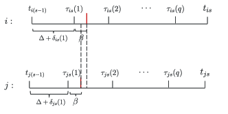
The other sub-system comprising agent ’s private estimator, is a “local parameter estimator” whose function is to generate estimates of at each of agent ’s preselected event times . Here is an ascending sequence of event times with a fixed spacing of time units between any two successive event times. In this section it is assume that , and consequently that all event time sequences are the same222It is easy to generalize the results in this section to the case when event times are not evenly spaced provided that the spacings between successive pairs of event times remains positive and bounded.. Thus Between event times, each is generated using the equation
| (5) |
Motivation for the development of the local parameter estimator whose purpose is to enable agent to estimate over the event time interval , stems from the fact that the equations
admit a unique solution, namely . Existence follows from (4) whereas uniqueness is a consequence of the assumption of joint observability.
The existence and uniqueness of suggest that an approximate value of can be obtained after a finite number of iterations - say - using the linear equation solver discussed in[32]. Having obtained such an approximate value of , denoted below by , the desired estimate of can be taken as
| (6) |
This is the
architecture which will be considered.
The computations needed to update agent ’s estimate of
are carried out by agent during the event
time interval . This is done using a local
parameter estimator which generates a sequence of auxiliary
states where is a
positive integer to be specified below. The sequence is initialized
by setting
| (7) |
and is recursively updated by agent at local iteration times known only to agent . It is assumed that the together with the initialization are of the form
| (8) |
where is a sequence of small deviations which satisfy
| (9) |
Here is a small nonnegative number whose constraints will be described below and is a positive number satisfying
The signal
is agent ’s updated estimate of
and is used to define
as in (6).
The transfer of information between agents which is needed to
generate the , is carried out
asynchronously
as follows.
For and , agent broadcasts
at time
where is any prescribed nonnegative number chosen smaller than .
It is assumed
that the bounds , appearing in (9) are
small enough so that there exist and satisfying
| (10) |
These inequalities ensure that for , a broadcast by any agent at time will occur within the reception interval of agent . Fig. 1 provides an example of the update and communication times of two different different agents and .
Accordingly, agent is a data source or just source for agent on if agent is in the reception range of agent at time . Let denote the set of labels of such agents; that is
| (11) |
Note that , for all so is never empty. Clearly agent can use the signals , to compute .
Prompted by [32], the update equation used to recursively generate the during agent ’s th event time interval is given by
| (12) |
where , is an averaged state
| (13) |
and is the number of labels in . The overall private estimator for agent is thus described by the equations (3), (5) - (8) and (11) - (13). In summary, initialize , randomly. For , . Then for , the algorithm of the hybrid estimator for anget is shown in Algorithm 1.
In order to complete the definition of the hybrid observer, it is necessary to specify values of the and . Towards this end, suppose that as a design goal it is desired to pick the and so that all state estimation errors
| (14) |
converge to zero as fast as does where is some desired convergence rate. The would then have to be chosen using spectrum assignment or some other technique so that the matrix exponentials all converge to zero at least as fast as does. This of course can be accomplished because each matrix pair is observable. In the sequel it will be assumed that for some preselected positive number , the have been chosen so that for the local observer estimation errors satisfy
| (15) |
where the are nonnegative constants and denotes the two-norm.
To describe how to define an appropriate value of to attain the desired convergence rate for the state estimation errors , it is necessary to take some preliminary steps. First, for each , let denote the orthogonal projection on the unobservable space of . It is easy to see that . Moreover, because of the assumption of joint observability,
| (16) |
Next, let denote the set of all products of the form where each projection matrix in occurs in each of such product at least once. Note that is a closed subset of . Since each projection matrix has a two-norm which is no greater than , each matrix has a two-norm less than or equal to . Thus is also a bounded and thus compact subset. In fact, each product in actually has two-norm strictly less than . This is a consequence of (16) and the requirement that each matrix in must occur in each product in at least once {Lemma 2, [33]}. These observations imply that maximum of the two-norms of the matrices in , namely
| (17) |
exists and is a real non-negative number strictly less than 333It is worth noting that although the matrices used in defining the are not uniquely determined by the unobservable spaces of the pairs , the orthogonal projection matrices nonetheless are. Thus the set used in the definition of in (17) ultimately depends only on the family of unobservable spaces of the pairs and not on the particular manner in which the are chosen. Just how to explicitly characterize this dependence is a topic for future research.. This in turn implies that the attenuation constant
| (18) |
is also a real non-negative number strictly less than . As will become evident below {cf. (40) and Lemma 5}, in the idealized case when all and are zero, for any integer and any given value of satisfying
| (19) |
the value of the signal
is attenuated by at least a factor after iterations during each event - time interval ; i.e., for ,
It will soon be apparent, if it is not already from (6), (7) and (14), that over each event- time interval ,
| (20) | |||||
Since each event - time interval is of length , to achieve an exponential convergence rate of in the idealized case, it is necessary to pick so that (19) holds where is any integer satisfying . In other words, the requirement on is that (19) hold where
| (21) |
with here denoting, for any nonnegative number , the smallest integer . The following theorem, which applies to the synchronous case when all of the are zero, {but not necessarily the } summarizes these observations.
Theorem 1.
This theorem will be proved in the next section. Several comments are in order. First, the attenuation of by over an event time interval is not likely to be tight and a larger attenuation constant can almost certainly be expected. This is important because the larger the attenuation constant the smaller the required value of needed to achieve a given convergence rate. Second, the hypothesis that strongly connected is almost certainly stronger than is necessary, the notion of a repeatedly jointly strongly connected sequence of graphs [33] being a likely less stringent alternative.
To deal with the asynchronous case when at least some of the are nonzero, it is necessary to assume that is constant on each of the time intervals
| (23) |
where
| (24) |
For this assumption to make sense, these intervals cannot overlap. The following lemma establishes that this is in fact the case.
Lemma 1.
Proof of Lemma 1: Fix . Note that because of (10). This implies that and thus that and are disjoint. Since this holds for all satisfying , all are disjoint.
From (10), and . These inequalities imply that and respectively. From this it follows that , that and thus that .
We are led to the asynchronous version of Theorem 22.
Theorem 2.
Asynchronous case: Suppose the , satisfy (10) and that the neighbor graph is constant on each interval and strongly connected for all . Let and be defined by (17) and (18) respectively and suppose that satisfies (22). Then as in Theorem 22, each state estimation , of the hybrid observer defined by(3), (5) - (8) and (11) - (13), tends to zero as fast as does.
The proof of this theorem will be given in the next section. Notice that the asynchronous case here can not be recognized in a discrete-time setting with a discrete-time clock shared by all agents considering delays[34].
2.1 A special case
It is possible to relax somewhat the lower bound (22) for to achieve exponential convergence in the special case when the neighbor graph is symmetric and strongly connected for all . This can be accomplished by replacing the straight averaging rule defined by (13), with the convex combination rule
| (25) |
where is the number of labels in .
To proceed, let denote the set of all symmetric and strongly connected, graphs on vertices. Each graph uniquely determines a matrix where is the Laplacian of the simple, weakly connected {undirected} graph determined by . It is easy to see that is a symmetric, doubly stochastic matrix with positive diagonals and that is its graph. The connection between these matrices and the update rule defined by (25) will become apparent later when assumptions are made which enable us to identify the subsets appearing in (25) with the neighbor sets of the neighbor graph {c.f. Lemmas 36 and 3}. Later in this paper it will also be shown that is a contraction in the two norm {Lemma 6}. This means that
| (26) |
is a nonnegative number less than one.
As will become clear, to achieve a convergence rate of , it is sufficient to pick large enough to that . In other words, in the special case when is symmetric and strongly connected for all time, instead of choosing to satisfy (22), to achieve an exponential convergence rate of it is enough to choose to satisfy the less demanding constraint
| (27) |
Justification for this claim is given in §3. Choosing in this way is easier that choosing according to (22) because the computation of is less demanding than the computation of and consequently . On the other hand, this special approach only applies when the neighbor graph is symmetric.
3 Analysis
The aim of this section is to analyze the behavior of the hybrid observer defined in the last section. To do this, use will be made of the notion of a “mixed matrix norm” which will now be defined. For any positive integers , , and , let denote the real - dimensional vector space of block partitioned matrices where each block is a matrix. By the mixed matrix norm of written , is meant the infinity norm of the matrix where is the two-norm of . For example, with denoting the “stacked” state estimation error the quantity mentioned in the last section, is , the mixed matrix norm of . It is straight forward to verify that is in fact a norm and that this norm is sub-multiplicative [33].
Recall that the purpose of agent ’s local parameter estimator defined by (7), (12), and (13) is to estimate after executing iterations during the th event time interval of agent . In view of this, we define the parameter error vectors for ,
| (28) |
for all . This, (7), and the definition of in (14) imply that
| (29) |
In addition, from (5), (6) and (14) it is clear that that
| (30) |
To derive the update equation for as ranges from to , we first note from (13) that
| (31) |
Next note that because of (4) and (12)
From this and (31) it follows that for ,
| (32) |
where as before, . These are the local parameter error equations for the hybrid observer.
The next step in the analysis of the system is studied the evolution of the all-agent parameter error vector
Note first that because of (29) and (30)
| (33) |
and
| (34) |
where is the all-agent state estimation error vector
| (35) |
and .
In order to develop an update equation for as ranges from to , it is necessary to combine the update equations in (32) into a single equation and to do this requires a succinct description of the graph determined by the sets defined in (11). There are two cases to consider: the synchronous case which is when all of the and the asynchronous case when some or all of the may be non-zero. The following lemmas cover both cases.
Lemma 2.
Synchronous Case: Suppose . Then for any fixed value of satisfying (10), including ,
| (36) |
Proof of Lemma 36: By hypothesis all . Clearly (10) can be satisfied with . Moreover from (8) and (9) and the assumption that , it follows that , so . From this and (11) it follows that (36) is true.
The following lemma asserts that (36) still holds in the asynchronous case when some of the are nonzero, provided is constant on each interval .
Proof of Lemma 3: Fix , and . In light of (8), (9) and the assumption that , it is clear that for any ,
Moreover, . But by assumption, is constant on which means that is constant on .Therefore . From this and the definition of in (11), it follows that (36) is true.
In summary, Lemmas 36 and 3 assert that (36) holds in the synchronous case when all , or alternatively in the asynchronous case when the neighbor graph is constant on each interval Because of this, the following steps to obtain an update equation for apply to both cases.
Equation (36) implies that the graphs determined by the are the neighbor graphs . Since is assumed to be strongly connected for all , each of these neighbor graphs is strongly connected. These graphs are used as follows.
Let denote the set of all directed graphs on vertices which have self-arcs at all vertices. Note that is a finite set and that . Each graph uniquely determines a so-called “flocking-matrix” which is an stochastic matrix of the form , where and are respectively the adjacency matrix and diagonal in-degree matrix of of ; is nonsingular because each graph in has self-arcs at all vertices.
For and , let denote the flocking matrix determined by . Then (32) implies for that
| (37) |
where
| (38) |
, and is the identity. Thus for ,
| (39) |
where is the state transition matrix defined by
| (40) |
for and by for . From this, (33) and (34) it follows that for , the all-agent state estimation error satisfies
| (41) |
where
| (42) | |||||
| (43) |
To determine the convergence properties of as use will be made of the following lemma which gives bounds on the norms of the coefficient matrices and appearing in (41).
Lemma 4.
Suppose that satisfies the inequality given in Theorem 22. Then
| (44) | |||||
| (45) |
In order to justify the bound on the norm of given in (44), use will be made of the following lemma. which is a simple variation on a result in [33].
Lemma 5.
Let denote the set of all flocking matrices determined by those graphs in which are strongly connected. For any set of flocking matrices in
| (46) |
where is the attenuation constant
Proof of Lemma 5: Fix , set and let and be flocking matrices in . Then
But for any flocking matrix , where is the infinity norm. From this, the sub-multiplicative property of the mixed matrix norm, and the fact that , it follows that
In view of equation (26) of [33],
Therefore (46) is true.
Proof of Lemma 4: Lemma 5 implies that if for a given integer , if then for any ,
| (47) |
Therefore by (40) and (42), if is so chosen, then . Thus by picking so large that
| (48) |
and then setting one gets (44). The requirement on determined by (48) is equivalent to the requirement on determined by (21). It follows that (44) will hold provided satisfies the inequality given in Theorem 22.
Recall that and that for any stochastic matrix . From this and the sub-multiplicative property of the mixed matrix norm it follows that the matrix defined by (40) satisfies
| (49) |
It is obvious at this point that because (36) holds in both the synchronous and asynchronous cases, the same arguments can be used to prove both Theorem 22 and Theorem 2.
Proof of Theorems 22 and 2: In view of (41) and Lemma 4 it is possible to write
where . Therefore
| (50) |
To deal with the term involving in (50), we proceed as follows. Note first from (15) that
Thus for . It follows from this and the definition of in (38) that
where . Thus for
Using (50) there follows
| (51) |
where
Fix . In view of (51) and the definition of in (35),
But for , ; consequently for the same values of . Therefore
so
Therefore for and
Now for ,
so
Since this holds for all
which proves that the state estimation errors , all converge to zero as fast as does.
3.1 Special case
We now turn to the special case mentioned in §2.1. In this case the definition of the state-transition matrix appearing in (39) changes from (40) to
| (52) |
for , and with graph .
Although the formula for , namely (41), and the definitions of and in (42) and (43) are as before, the bounds for and and given by (44) and (45) no longer apply. To proceed, use will be made of the following lemma.
Lemma 6.
Let be an doubly stochastic matrix with positive diagonals and a strongly connected graph. Suppose that , is a set of orthogonal projection matrices such that
| (53) |
Then the matrix is a contraction in the -norm where .
Proof: Write for and note that is doubly stochastic with positive
diagonals and a strongly connected graph.
Since , it must be true that
that
. Moreover because
is stochastic; thus . Hence it is enough to prove that or equivalently that
Suppose that or equivalently that
for some nonzero vector . Clearly PSS’Px = Px which implies that and thus that
Therefore . From this and Lemma 1 of [35] it follows that
.
Now is stochastic. Moreover its graph is strongly connected because
has a strongly connected graph and positive diagonals, as does . Thus by the Perron Frobenius theorem,
has exactly one eigenvalue at and all the rest must be inside the unit circle; in addition the
eigenspace for the eigenvalue must be spanned by the one-vector . Therefore
for some nonzero scalar . Therefore which implies that
, But this is impossible because of (3).
The following lemma gives the bounds on and for the special case under consideration.
Lemma 7.
Suppose that satisfies (27). Then
| (54) | |||||
| (55) |
Proof: Lemma 6 implies that for each , . Moreover, where is chosen according to (26). From this and the sub-multiplicative property of the two norm it follows that
Therefore by (42) and (52), if is so chosen to satisfy (27), then
Thus (54) is true. Recall that and for . From this and the sub-multiplicative property of the two norm, the matrix defined by (52) satisfies
Other than the modifications in the bounds on and given in the above lemma, everything else is the same for both the synchronous and asynchronous versions of the problem. So what one gains in this special case is exponential convergence at a prescribed rate with a smaller value of .
4 Event-time Mismatch - A Robustness Issue
In the preceding section it was shown that the hybrid observer under discussion will function correctly if local iterations are performed synchronously across the network no matter how fast the associated neighbor graph changes, just so long as it is always strongly connected. Correct performance is also assured in the face of asynchronously executed local iterations across the network during each event time interval, provided the neighbor graph changes in a suitably defined sense. Implicitly assumed in these two cases is that the event time sequences of all agents are the same. The aim of this section is to explain what happens if this assumption is not made. For simplicity, this will only be done for the case when differing event time sequences are the only cause of asynchronism. As will be seen, the consequence of event-time sequence mismatches turns out to be more of a robustness issue than an issue due to unsynchronized operation. In particular, it will become apparent that if different agents use slightly different event time sequences then asymptotically correct state estimates will not be possible unless is a stability matrix. While at first glance this may appear to be a limitation of the distributed observer under consideration, it is in fact a limitation of virtually all state estimators, distributed or not, which are not used in feedback-loops. Since this easily explained observation is apparently not widely appreciated, an explanation of this simple fact will be given at the end of this section.
There are two differences between the setup to be considered here and the setup considered in the last section. First it will now be assumed that the local deviation times appearing in (8) are all zero. Thus in place of (8) the local iteration times for agent on
| (56) |
Second instead of assuming that the initializations of the agents’ event time sequences are all zero, it will be assumed instead that each is a small number known only to agent which lies in the interval where, as before, is a small nonnegative number. This means that even though the event time sequences of all agents are still periodic with period , the sequences are not synchronized with each other. As before it is assumed that within event time interval , agent broadcasts iterate at time . To ensure that this time falls within the reception interval of each agent , it will continue to be assumed that (10) holds. Apart from these modifications the setup to be considered here is the same as the one considered previously. As a consequence, many of the steps in the analysis of the hybrid observers performance are the same as they were for the previously considered case.
Our first objective is to develop the relevant equations for the local parameter error vector defined by (28). Although (29) and (30) continue to hold without change, (32) requires modification. To understand what needs to be changed, it is necessary to first derive a relationship between and . Towards this end, note that
because for all . From this and (5) it follows that
Hence (13) can now be used to obtain
| (57) |
where
| (58) |
Next note that because of (4) and (12)
From this and (57) it follows that
| (59) |
which is the modified version of (32) needed to proceed. The difference between (32) and (59) is thus the inclusion in (59) of the term .
The assumption that the event time sequences of the agents may start at a different time requires us to make the same assumption as before about the neighbor graph , namely that it is constant on each interval . The assumption makes sense in the present context for the same reason as before, specifically because the interval defined by (23) do not overlap. This, in turn, is because the bounds have been assumed to satisfy (10) which guarantees that Lemma 1 continues to hold.
The next step in the analysis of the hybrid observer is to study the evolution of the all-agent parameter error vector
As before, (33) and (34) continue to hold where is the all - agent state estimation error defined by (35). A simple modification of the proof of Lemma 3 can be used to establish the lemma’s validity in the present context. Consequently a proof will not be given. The lemma enables us to combine the individual update equations in (59), thereby obtaining the update equation
where
| (60) |
The steps involved in doing this are essentially the same as the steps involved in deriving (37). Not surprisingly, the only difference between (37) and (60) is the inclusion in the latter of the term .
From (33), (34), and (60) it follows at once that the all-agent state estimation error vector satisfies
| (61) |
where and are as defined in (42) and (43) respectively, and
The following lemma gives a bound on the mixed matrix norm of .
Lemma 8.
Suppose that satisfies the inequality given in Theorem 22. Then
| (62) |
Note that this bound is small when is small. This means that small deviations of the agent’s event time sequences from the nominal event time sequence produce small effects on the error dynamics in (61), provided of course is well behaved; i.e., is a stability matrix! More will be said about this point below.
In general, for any real square matrix , and real numbers and
so
By assumption and . But and . Thus and . Therefore
so
In view of (49) and the definition of , . It follows that (62) holds.
Taking the construction leading to (50) as a guide, it is not difficult to derive from (61) the inequality
| (63) |
where is as defined just below (51) and . Comparing (51) to (63), we see that the effect of the change in assumptions leads to the inclusion in (63) of the term involving .
At this point there are two distinct cases to consider - either converges to zero or it does not. Consider first the case when converges to zero. Then there must be positive constants and such that . By treating the term involving in (63) in the same manner as the term involving in (51) was treated, one can easily conclude that for a suitably defined constant
if , or
if . If the former is true, then the same arguments as were used in the last section can be used to show that the state estimations errors converge to zero as fast as does. On the other hand, if the latter is true, by similar reasoning can easily be shown to converge to zero as fast as does. Note that in this case, if is small, the effect of the resulting slow convergence of will to some extent be mitigated by the smallness of , so even with small , the performance of the hybrid observer may be acceptable for sufficiently small perturbations of the start times of the event time sequences from .
In the other situation, which is when is not a stability matrix, the hybrid observer cannot perform acceptably except possibly if finite time state estimation is all that is desired and is sufficiently small.
Key Point: This limitation applies not only to the hybrid observer discussed in this paper, but to all state estimators, centralized or not, including Kalman filters which are not being used in feedback loops.444Some of the adaptive observers developed in the past may be an exception to this, but such observers invariably require persistent excitation to achieve exponential convergence.
Experience has shown that this limitation is not widely recognized, despite its
simple justification. Here is the justification.
Suppose one is trying to obtain an estimate of the
state
of a single-channel, observable linear system , using an observer
but approximately correct values of and
- say and - upon which to base the observer design are known.
The observer would then be a linear system
of the form
| (64) |
with chosen to exponentially stabilize . Then it is easy to see that the state estimation error must satisfy
Therefore if is not a stability matrix and either is not exactly equal to or is not exactly equal to , then instead of converging to zero, the state estimation error will grow without bound for almost any initialization. In other words, with robustness in mind, the problem of trying to obtain an estimate of the state of a linear system with an “open-loop” state estimator, does not make sense unless is a stability matrix. Of course, if one is trying to use a state estimator generate an estimate of the state of the forced linear system
where is a stability matrix, this problem does not arise, but to accomplish this one has to change the estimator dynamics defined in (64) to
While this modification works in the centralized case, it cannot be used in the decentralized case as explained in [36]. In fact, until recently there appeared to be only one of distributed observer which could be used in a feedback configuration thereby avoiding the robustness issue just mentioned [36]. However, recent research suggests other approach may emerge [37].
5 Resilience
By a (passively) resilient algorithm for a distributed process is meant an algorithm which, by exploiting built-in network and data redundancies, is able to continue to function correctly in the face of abrupt changes in the number of vertices and arcs in the inter-agent communication graph upon which the algorithm depends. In this section,it will be shown that the proposed estimator can cope with the situation when there is an arbitrary abrupt change in the topology of the neighbor graph such as the loss or addition of an arc or a vertex provided connectivity is not lost in an appropriately defined sense.
Consider first the situation when there is a potential loss or addition of arcs in the neighbor graph. Assume the neighbor graph is -arc redundantly strongly connected in that the graph is strongly connected and remains strongly connected after any arcs are removed. With this assumption, strong connectivity of the neighbor graph and jointly observability of the system are ensured when any arcs are lost. Alternatively, if any number of new arcs are added, strong connectivity and joint observability are clearly still ensured. Thus, in the light of Theorem 22, whenever arcs are lost from or added to the neighbor graph, the hybrid estimator under consideration will still function correctly without the need for any “active” intervention such as redesign of any of the or readjustment of . In fact, Theorem 22 guarantees that correct performance will prevail, even if arcs change over and over, no matter how fast, just so long as strong connectivity is maintained for all time.
Consider next the far more challenging situation when at some time there is a loss of vertices from the neighbor graph For this situation, only preliminary results currently exist. One possible way to deal with this situation is as follows.
As a first step, pick the as before, so that all local observer state estimator errors converge to zero as fast as does. Next, assume that the neighbor graph is -vertex redundantly strongly connected in that it is strongly connected and remains strongly connected after any vertices are removed. Assume in addition that the system described by (1), (2) is redundantly jointly observable in that the system which results after any output measurements have been deleted, is still jointly observable. Let denote the family of all nonempty subsets such that each subset contains at least vertices. Thus each loss of at most vertices results in a strongly connected subgraph of for some subset ; call this subgraph . Correspondingly, let denote the multi-channel linear system which results when those outputs are deleted from (1), (2). Thus is a jointly observable multi-channel linear system whose channel outputs are the . Fix .
Fix and let denote the number of vertices in . Since is jointly observable it is possible to compute a number which satisfies (17). Using the pair in place of the pair in (18) and (22), it is possible to calculate a value of , for which (22) holds. In other words, for this value of , henceforth labelled Theorem 22 holds for the multichannel system and neighbor graph . By then picking
one obtains a value of for which Theorem 22 holds for all pairs as ranges over . Suppose a hybrid observer using is implemented. Suppose in addition that at some time , for some specific , agents with labels in stop functioning. Clearly the remaining agents with labels in will be able to deliver the desired state estimates with the prescribed convergence rate bounds. In this sense, the observer under consideration is resilient to vertex losses. However, unlike the loss or addition of edges mentioned above, no claim is being made at this point about what might happen if some or all of the lost vertices rejoin the network, especially if this loss-gain process is rapidly reoccurring over and over as time evolves.
A similar approach can be used to deal with the situation when at some time , the network gains some additional agents. In this case one would have to specify all possibilities and make sure that for each one, one has a strongly connected graph and a jointly observable system.
A little thought reveals that what makes it possible to deal with a change in the number of vertices in this way, is the fact that there is a single scalar quantity, namely , with the property that for each possible graphical configuration resulting from an anticipated gain or loss of vertices, there is a value of large enough for the distributed observer to perform correctly and moreover if is assigned the maximum of these values then the distribute observer will perform correctly no matter which of the anticipated vertex changes is actually encountered. Since the distributed observers described in [23, 24, 26] also require the adjustment of only a single scalar-valued quantity for a given neighbor graphs, the same basic idea just described can be used to make the observers in [23, 24, 26] resilient to a one-time gain or loss of the number of vertices on their associated neighbor graph. On the other hand, some distributed observers such as the ones described in [15, 2, 38] are not really amenable to this kind of generalization because for such observers changes in network topology require completely new designs involving the change of many of the observer’s parameters. There are also papers [39, 40] deal with sensor attacks, where a malicious attacker can manipulate their observations arbitrarily when each sensor only has one dimensional measurement.
6 Simulation
The following simulations are intended to illustrate (i) the performance of the hybrid observer in the face of system noise, (ii) the robustness of the hybrid observer with respect to variations of event time sequences, and (iii) resilience of the hybrid observer to the loss or gain of an agent. Consider the four channel, four-dimensional, continuous-time system described by the equations , where
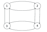
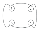
and is the th unit row vector in . Note that is a stable matrix with two eigenvalues at and a pair of complex eigenvalues at . While the system is jointly observable, no single pair is observable. However the system is “redundantly jointly observable” in that what remains after the removal of any one output , is still jointly observable. For the first two simulations is switching back and forth between Figure 2(a) and Figure 2(b), and for the third simulation the neighbor graph is as shown in Figure 2(a). Both graphs are strongly connected, and the graph in Figure 2(a) is redundantly strongly connected in that it is strongly connected and remains strongly connected after any one vertex is removed.
Suppose for this system. To achieve a convergence rate of
, and are chosen to be and
respectively.
For agent 1: ,
For agent 2: ,
For agent 3: ,
For agent 4: ,
In all four cases the local observer convergence rates are all .
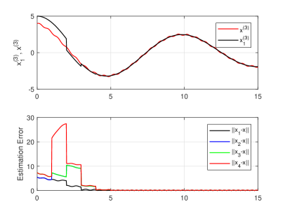
This system was simulated with as the initial state of the process, , , , and as the initial states of the four local observers, , and as the initial estimates of the four local estimators.
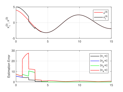
Three simulations were performed. The first is intended to demonstrate performance in the face of system noise. For this a modified process dynamic of the form is assumed where and is system noise. Traces of this simulation are shown in Figure 3 where and denote the third components of and respectively. Only the trajectory of is plotted because for agent only the third component is unobservable, and all the other components are observable.
The second simulation, which is without system noise, is intended to demonstrate the hybrid observer’s robustness against a small change in the event time sequence of one of the agents. The change considered presumes that the event times of agent 4 occur time units before the the event times of the other three agents. Traces of this simulation are shown in Figure 4.
The third simulation, also without system noise, is intended to demonstrate the hybrid observer’s resilience against the disappearance of agent 4 at time and also against agent ’s re-emergence at time . Traces of this simulation are shown in Figure 5.
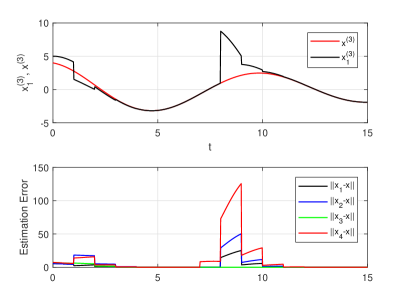
Disruption appearing at the beginning of the traces for all three simulations are due to initial conditions and are not important. In the third simulation, the loss of agent 4 at does not appear to have any impact whereas the trace shows that the re-emergence of agent 4 at briefly effects performance. While the claims in this paper do not consider the possibility of of agent re-emergence, it is not surprising that this event does not cause misbehavior because the time between the loss and gain of the agent, namely time units, is large compared to the time constants of the observer. Clearly much more work needs to be done here to better understand rapidly occurring and re-occurring losses and gains of agents.
7 Concluding Remarks
One of the nice properties of the hybrid observer discussed in this paper is that it is resilient. By this we mean that under appropriate conditions it is able to continue to provide asymptotically correct estimates of , even if communications between some agents break down or if one or several of the agents joins or leaves the network. The third simulation provides an example of this capability. As pointed out earlier, further research is needed to more fully understand observer resilience, especially the situation when agents join or leave the network.
Generally one would like to choose “small” to avoid unnecessarily large error overshooting between event times. Meanwhile it is obvious from (20) that the larger the number and consequently the number of iterations on each event-time interval, the faster the convergence. Two considerations limit the value of - how fast the parameter estimators can compute and how quickly information can be transmitted across the network. We doubt the former consideration will prove very important in most applications, since digital processors can be quite fast and the computations required are not so taxing. On the other hand, transmission delays will almost certainly limit the choice of . A model which explicitly takes such delays into account will be presented in another paper.
A practical issue is that the development in this paper does not take into account measurement noise. On the other hand, the observer provides exponential convergence and this suggests that if noisy measurements are considered, the observer’s performance will degrade gracefully with increasing noise levels. Of course one would like an “optimal” estimator for such situations in the spirit of a Kalman filter. Just how to formulate and solve such a problem is a significant issue for further research.
This work was supported by NSF grant 1607101.00, AFOSR grant FA9550-16-1-0290, and ARO grant W911NF-17-1-0499.
References
- [1] L. Wang, A. S. Morse, D. Fullmer, and J. Liu. A hybrid observer for a distributed linear system with a changing neighbor graph. In Proceedings of the 2017 IEEE Conference on Decision and Control, pages 1024–1029, 2017.
- [2] L. Wang and A. S. Morse. A distributed observer for an time-invariant linear system. IEEE Transactions on Automatic Control, 63(7):2123–2130, 2018.
- [3] Reza Olfati-Saber. Distributed Kalman filter with embedded consensus filters. Proceedings of the 44th IEEE Conference on Decision and Control, and the European Control Conference, CDC-ECC ’05, pages 8179–8184, 2005.
- [4] Reza Olfati-Saber. Distributed Kalman filtering for sensor networks. In Proceedings of the 46th IEEE Conference on Decision and Control, pages 5492–5498, 2007.
- [5] Reza Olfati-Saber. Kalman-Consensus Filter : Optimality, stability, and performance. Proceedings of the 48h IEEE Conference on Decision and Control, and the 28th Chinese Control Conference, pages 7036–7042, dec 2009.
- [6] Usman A Khan, Soummya Kar, Ali Jadbabaie, and José M.F. Moura. On connectivity, observability, and stability in distributed estimation. In Proceedings of the IEEE Conference on Decision and Control, pages 6639–6644, 2010.
- [7] U. A. Khan and Ali Jadbabaie. On the stability and optimality of distributed Kalman filters with finite-time data fusion. In Proceedings of the 2011 American Control Conference, pages 3405–3410, 2011.
- [8] Jaeyong Kim, Hyungbo Shim, and Jingbo Wu. On distributed optimal Kalman-Bucy filtering by averaging dynamics of heterogeneous agents. In Proceedings of the 55th IEEE Conference on Decision and Control, pages 6309–6314, 2016.
- [9] Jingbo Wu, Anja Elser, Shen Zeng, and Frank Allgöwer. Consensus-based Distributed Kalman-Bucy Filter for Continuous-time Systems. IFAC-PapersOnLine, 49(22):321–326, 2016.
- [10] Reza Olfati-Saber and Parisa Jalalkamali. Coupled distributed estimation and control for mobile sensor networks. IEEE Transactions on Automatic Control, 57(10):2609–2614, 2012.
- [11] Mohammadreza Doostmohammadian and Usman A. Khan. On the genericity properties in distributed estimation: Topology design and sensor placement. IEEE Journal of Selected Topics in Signal Processing, 7(2):195–204, 2013.
- [12] Usman A. Khan and Ali Jadbabaie. Collaborative scalar-gain estimators for potentially unstable social dynamics with limited communication. Autom., 50:1909–1914, 2014.
- [13] Shinkyu Park and NC Martins. An augmented observer for the distributed estimation problem for LTI systems. In Proceedings the 2012 American Control Conference, pages 6775–6780, 2012.
- [14] Shinkyu Park and Nuno C. Martins. Necessary and sufficient conditions for the stabilizability of a class of LTI distributed observers. In Proceedings of the 51st IEEE Conference on Decision and Control, pages 7431–7436, 2012.
- [15] Shinkyu Park and Nuno C Martins. Design of Distributed LTI Observers for State Omniscience. IEEE Transactions on Automatic Control, 62(2):561–576, 2017.
- [16] Aritra Mitra and Shreyas Sundaram. Distributed Observers for LTI Systems. IEEE Transactions on Automatic Control, 63(11):3689–3704, 2018.
- [17] Behçet Açikmeşe, Milan Mandić, and Jason L Speyer. Decentralized observers with consensus filters for distributed discrete-time linear systems. Automatica, 50(4):1037–1052, 2014.
- [18] Valery A. Ugrinovskii. Distributed robust estimation over randomly switching networks using consensus. Automatica, 49:160–168, 2013.
- [19] Álvaro Rodríguez del Nozal, Pablo Millán, Luis Orihuela, Alexandre Seuret, and Luca Zaccarian. Distributed estimation based on multi-hop subspace decomposition. Automatica, 99:213–220, 2019.
- [20] Francisco Castro Rego, Ye Pu, Andrea Alessandretti, A. Pedro Aguiar, António M. Pascoal, and Colin N. Jones. A distributed luenberger observer for linear state feedback systems with quantized and rate-limited communications. IEEE Transactions on Automatic Control, 66(9):3922–3937, 2021.
- [21] Shih-Ho Wang Shih-Ho Wang and E Davison. On the stabilization of decentralized control systems. IEEE Transactions on Automatic Control, 18(5):473–478, 1973.
- [22] J. P. Corfmat and A. S. Morse. Decentralized control of linear multivariable systems. Automatica, 12(5):479–497, September 1976.
- [23] Taekyoo Kim, Hyungbo Shim, and Dongil Dan Cho. Distributed Luenberger Observer Design. In Proceedings of the 55th IEEE Conference on Decision and Control, pages 6928–6933, Las Vegas, USA, 2016.
- [24] Weixin Han, Harry L. Trentelman, Zhenhua Wang, and Yi Shen. A simple approach to distributed observer design for linear systems. IEEE Transactions on Automatic Control, 64(1):329–336, 2019.
- [25] Weixin Han, Harry L. Trentelman, Zhenhua Wang, and Yi Shen. Towards a minimal order distributed observer for linear systems. Systems and Control Letters, 114:59–65, 2018.
- [26] L. Wang, J. Liu, and A. S. Morse. A distributed observer for a continuous-time linear system. In Proceedings of 2019 American Control Conference, pages 86–89, Philadelphia, PA, USA, July 2019.
- [27] Jin Gyu Lee and Hyungbo Shim. A distributed algorithm that finds almost best possible estimate under non-vanishing and time-varying measurement noise. IEEE Control Systems Letters, 4(1):229–234, 2020.
- [28] L. Wang, J. Liu, A. S. Morse, and B. D. O. Anderson. A distributed observer for a discrete-time linear system. In Proceedings of the 2019 IEEE Conference on Decision and Control, pages 367–372, 2019.
- [29] Y. Li, S. Phillips, and R.G. Sanfelice. Robust Distributed Estimation for Linear Systems under Intermittent Information. IEEE Transactions on Automatic Control, 63(4):1–16, 2018.
- [30] Aritra Mitra, John A Richards, Saurabh Bagchi, and Shreyas Sundaram. Finite-Time Distributed State Estimation over Time-Varying Graphs : Exploiting the Age-of-Information. 2018. arXiv:1810.06151 [cs.SY].
- [31] L. Wang and A. S. Morse. A distributed observer for a continuous-time, linear system with a time-varying graph. arXiv:2003.02134v1, mar 2020.
- [32] L. Wang, D. Fullmer, and A. S. Morse. A distributed algorithm with an arbitrary initialization for solving a linear algebraic equation. In Proceedings of the 2016 American Control Conference (ACC), pages 1078–1081, July 2016.
- [33] S. Mou, J. Liu, and A. S. Morse. An distributed algorithm for solving a linear algebraic equation. IEEE Transactiona on Automatic Control, pages 2863–2878, 2015.
- [34] Mohammadreza Doostmohammadian, Usman A. Khan, Mohammad Pirani, and Themistoklis Charalambous. Consensus-based distributed estimation in the presence of heterogeneous, time-invariant delays. IEEE Control Systems Letters, 6:1598–1603, 2022.
- [35] L. Wang, D. Fullmer, and A. S. Morse. A distributed algorithm with an arbitrary initialization for solving a linear algebraic equation. In Proceedings of the 2016 American Control Conference, pages 1078–1081, 2016.
- [36] F. Liu, L. Wang, D. Fullmer, and A. S. Morse. Distributed feedback control of multi-channel linear systems. arXiv:1912.03890, 2020. under revision.
- [37] T. Kim, D. Lee, and H. Shim. Decentralized design and plug-and-play distributed control for linear multi-channel systems. arXiv:2011.09735, 2020.
- [38] Mohammadreza Doostmohammadian, Hamid R. Rabiee, Houman Zarrabi, and Usman A. Khan. Distributed estimation recovery under sensor failure. IEEE Signal Processing Letters, 24(10):1532–1536, 2017.
- [39] Chanhwa Lee, Hyungbo Shim, and Yongsoon Eun. On redundant observability: From security index to attack detection and resilient state estimation. IEEE Transactions on Automatic Control, 64(2):775–782, 2019.
- [40] Xingkang He, Xiaoqiang Ren, Henrik Sandberg, and Karl Henrik Johansson. How to secure distributed filters under sensor attacks. IEEE Transactions on Automatic Control, 67(6):2843–2856, 2022.