A Hybrid Position/Force Controller for Joint Robots

We consider a robotic arm with 6 DOFs. The equation of motion is

$$M(\bm{\theta})\ddot{\bm{\theta}}+C\dot{\bm{\theta}}+{\bm{g}}({\bm{\theta}})+J^{T}\pazocal{F}_{\rm ext}=\bm{\tau}\text{,}$$

(1)

where $\bm{\theta}\in\mathbb{R}^{6\times 1}$ is the joint angle vector, $J$ is the arm’s Jacobian matrix, $M({\bm{\theta}})$, $C({\bm{\theta}},\dot{\bm{\theta}})$, and $\bm{g}(\bm{\theta})$ are the mass matrix, Coriolis and centrifugal vector, gravity vector, respectively, and $\pazocal{F}_{\rm ext}=[\bm{m}^{T}_{\rm ext},\bm{f}^{T}_{\rm ext}]^{T}=[m_{x},m_{y},m_{z},f_{x},f_{y},f_{z}]^{T}$ is the wrench applied by the end-effector to the environment. The control input to the robot is $\bm{\tau}$, the torque applied to the joint motors.

The motion controller in the task space from [3] (pp. 195-197) is used. Define a smooth and invertible mapping from the joint space to task space $f:\bm{\theta}\in\mathbb{R}^{6\times 1}\to\bm{x}\in\mathbb{R}^{6\times 1}$. In this work, the joint space is mapped to the task space defined with the position and orientation of the end-effector, i.e., $\bm{x}=[\alpha,\beta,\gamma,x,y,z]^{T}$. Note that this mapping is not globally but locally invertible thus works in a region, so multiple mappings may be used for the entire joint space. The Jacobian $J_{f}$ with respect to $f$ is defined as

$$\dot{\bm{x}}=J_{f}\dot{\bm{\theta}}\text{,}\quad\quad J_{f}=\frac{\partial f}{\partial{\bm{\theta}}}\text{.}$$

(2)

Thus,

$$\ddot{\bm{x}}=\dot{J}_{f}\dot{\bm{\theta}}+J_{f}\ddot{\bm{\theta}}\quad\Rightarrow\quad\ddot{\bm{\theta}}=J_{f}^{-1}(\ddot{\bm{x}}-\dot{J}_{f}\dot{\bm{\theta}})\text{.}$$

(3)

The motion controller can be expressed as

$$\bm{\tau}=C\dot{\bm{\theta}}+{\bm{g}}({\bm{\theta}})+MJ_{f}^{-1}(\ddot{\bm{x}}_{d}+K_{v}\dot{\bm{x}}_{e}+K_{p}{\bm{x}}_{e}+K_{i}\int_{0}^{t}{\bm{x}}_{e}ds-\dot{J}_{f}\dot{\bm{\theta}})\textbf{,}$$

(4)

where ${\bm{x}}_{e}={\bm{x}}_{d}-{\bm{x}}$; ${\bm{x}}_{d}$ and ${\bm{x}}$ are the desired and actual configuration, respectively; $K_{v}$, $K_{p}$, and $K_{i}$ are the controller parameters and should be chosen properly to ensure stability [3] (pp. 198).

To introduce the hybrid controller, consider a task of cleaning a table with a robotic arm. The table surface is a plane parallel to the $x\text{-}y$ plane in world frame with the $z$ axis pointing upward. Therefore, for such a task, a hybrid controller is needed to manipulate the end-effector to move from point $A$ to point $B$ on the table while maintaining a downward force (i.e., in -$z$ direction).

Define the mapping $f:{\bm{\theta}}\to{\bm{x}}=[\alpha(t),\beta(t),\gamma(t),x(t),y(t),z(t)]^{T}$, where $x$, $y$, and $z$ are coordinates in world frame and the rest DOFs are orientation angles. We can decouple the 6 DOFs in the task space, i.e., the motion controller will be used to regulate $\{x(t),y(t),\alpha(t),\beta(t),\gamma(t)\}$ to track the reference trajectory and the force controller regulates the contact force in $z$ direction through manipulating $z(t)$. Let ${\bm{x}}_{d}=[\alpha_{d}(t),\beta_{d}(t),\gamma_{d}(t),x_{d}(t),y_{d}(t),z_{d0}]^{T}$ be the reference trajectory in the task space with $z_{r0}$ the initial $z$ position of the tip.

Plug Eqs.(4) and (3) into Eq. (1), we can obtain

$$\ddot{\bm{x}}_{e}+K_{v}\dot{\bm{x}}_{e}+K_{p}{\bm{x}}_{e}+K_{i}\int_{0}^{t}{\bm{x}}_{e}ds-J_{f}M^{-1}J^{T}\pazocal{F}_{\rm ext}=0\text{.}$$

(5)

Let $[\cdot]_{i}$ denote the $i$th elements of a vector and $u=J_{f}M^{-1}J^{T}\pazocal{F}_{\rm ext}$. Eq. (5) can be decomposed into two parts as follows.

$${[\ddot{\bm{x}}_{e}]}_{i}+K_{v}{[\dot{\bm{x}}_{e}]}_{i}+K_{p}{[{\bm{x}}_{e}]}_{i}+K_{i}\int_{0}^{t}{[{\bm{x}}_{e}]}_{i}ds-[u]_{i}=0\text{,}1\leq i\leq 5$$

(6)

$$[\ddot{\bm{x}}_{e}]_{6}+K_{v}{[\dot{\bm{x}}_{e}]}_{6}+K_{p}{[{\bm{x}}_{e}]}_{6}+K_{i}\int_{0}^{t}{[{\bm{x}}_{e}]}_{6}ds-[u]_{6}=0$$

(7)

Eq. (6) represents the motion error dynamics while Eq. (7) will be used for the force controller design. Note that $\pazocal{F}_{\rm ext}$ is not canceled in Eq. (5) since it is difficult to accurately measure the term $\pazocal{F}_{\rm ext}$ and there will be a delay in canceling the term resulting in some unexpected behaviors.

Remark 1. The force term $\pazocal{F}_{\rm ext}$ can be canceled (then $u=0$) if accurate sensors are available and the conclusion will not be affected. We are going to discuss the effect if this term is not canceled or just partially canceled.

Eq. (6) is the motion error dynamics after applying the motion controller Eq. (4). Here we explain how the term $\pazocal{F}_{\rm ext}$ affects the controller performance. If $\pazocal{F}_{\rm ext}$ is not canceled then $[u]_{i}=[J_{f}M^{-1}J^{T}\pazocal{F}_{\rm ext}]_{i}$; if $\pazocal{F}_{\rm ext}$ is not fully canceled, $[u]_{i}$ represents the residual term after canceling, then we can obtain the transfer function of the system with input $u_{i}(t)$ and output $y_{i}(t)=[X_{e}]_{i}$ from Eq. (6) as

$$G_{i}(s)=\frac{Y_{i}(s)}{U_{i}(s)}=\frac{s}{s^{3}+K_{v}s^{2}+K_{p}s+K_{i}}\text{.}$$

(8)

If $K_{v}$, $K_{p}$, and $K_{i}$ are chosen such that Eq. (8) is stable, it yields a low pass filter which has a very small gain in low frequency region. Thus, $u_{i}$ does not affect the tracking error $y_{i}$ much. In particular, when $s\to 0$, $G_{i}(s)\to 0$ which implies that constant $u_{i}$ cannot affect the output at all.

Let ${z}_{e}={z}_{d}-{z}_{t}={[{\bm{x}}_{e}]}_{6}$ where ${z}_{d}$ is the desired $z$ position and $z_{t}$ is the actual $z$ position of the end-effector. Let $f_{e}=f_{d}-f_{z}$, with $f_{d}$ the desired downward force and $f_{z}$ the actual downward force. We integrate another controller Eq. (10) with Eq. (7) as follows (Note that (9) is obtained by replacing ${[\bm{x}_{e}]}_{6}$ with ${z}_{e}$ in (7)).

	$\displaystyle\ddot{z}_{e}+K_{v}\dot{z}_{e}+K_{p}{z}_{e}+K_{i}\int_{0}^{t}{z}_{e}ds-(\epsilon f_{z}+\eta)=0$		(9)
	$\displaystyle u_{c}=\dot{z}_{d}=K_{p1}f_{e}+K_{i1}\int_{0}^{t}f_{e}ds\text{~{},}$		(10)

where $(\epsilon f_{z}+\eta)=[J_{f}M^{-1}J^{T}\pazocal{F}_{\rm ext}]_{6}$, $u_{c}$ is the input for the force controller. In Eq. (9), $f_{z}$ is extracted and the rest terms in $[J_{f}M^{-1}J^{T}\pazocal{F}_{\rm ext}]_{6}$ are accounted for with $\epsilon$ and $\eta$. Again, if $\pazocal{F}_{\rm ext}$ can be canceled, $\epsilon=0$, $\eta=0$. The reason why $f_{z}$ is extracted here is that $f_{z}$ can be very large thus dominates over other terms in $\pazocal{F}_{\rm ext}$ (i.e., $f_{x}$, $m_{x}$, etc.) when $f_{d}$ is large.

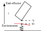
Controller Eq. (10) essentially indirectly regulates the contact force through adjusting the desired $z$ position. The block diagram of the force controller is shown in Fig. 1. We use a spring model to approximate the interaction dynamics between the tip and the environment. As seen in Fig. 2, let $q_{z}$ be the $z$ position of the contact point before contacting (before contacting there is no deformation at the contact point), the contact force can be computed with $f_{z}=\delta(k)({q_{z}}-z_{t})$, where

$$\begin{aligned} \delta(k)=\begin{cases}&k\text{~{}, if}~{}~{}q_{z}>z_{t}\\ &0\text{~{}, if}~{}~{}q_{z}\leq z_{t}\end{cases}\end{aligned}\text{.}$$

(11)

Sometimes the environment may be rigid and there is no deformation, the model can still work due to the flexibility of the robotic arm. When implementing the controller, $f_{z}$ can be read from the F/T sensor.

To obtain the closed-loop force error dynamics, the system state $W=[w_{1},\cdots,w_{6}]^{T}$ is defined as follows. For simplicity, it is assumed that $\dot{f}_{d}=0$, but this assumption can be removed and similar analysis can be carried out.

$$\begin{aligned} \begin{cases}w_{1}&=\int_{0}^{t}z_{e}ds\\ w_{2}&=z_{t}\\ w_{3}&=\dot{z}_{e}\\ w_{4}&=z_{d}\\ w_{5}&=\int_{0}^{t}f_{e}ds\\ w_{6}&=f_{e}\end{cases}\end{aligned}\Rightarrow\begin{aligned} \begin{cases}\dot{w}_{1}&=z_{e}=z_{d}-z_{t}=w_{4}-w_{2}\\ \dot{w}_{2}&=\dot{z}_{t}=\dot{z}_{d}-\dot{z}_{e}=u_{c}-w_{3}\\ &=-w_{3}+K_{i1}w_{5}+K_{p1}w_{6}\\ \dot{w}_{3}&=\ddot{z}_{e}=-K_{v}w_{3}-K_{p}(w_{4}-w_{2})\\ &~{}~{}-K_{i}w_{1}+(\epsilon f_{z}+\eta)~{}(\text{by Eq. (\ref{controller2_1})})\\ \dot{w}_{4}&=\dot{z}_{d}=u_{c}=K_{i1}w_{5}+K_{p1}w_{6}\\ \dot{w}_{5}&=f_{e}=w_{6}\\ \dot{w}_{6}&=\dot{f}_{e}=-\dot{f}_{z}\end{cases}\end{aligned}$$

(12)

The system state-space equation is

$$\begin{aligned} \dot{W}&=A_{w}W+BU_{w}\\ =&\begin{bmatrix}0&-1&0&1&0&0\\ 0&0&-1&0&K_{i1}&K_{p1}\\ -K_{i}&\epsilon\delta(k)+K_{p}&-K_{d}&-K_{p}&0&0\\ 0&0&0&0&K_{i1}&K_{p1}\\ 0&0&0&0&0&1\\ 0&0&-\delta(k)&0&\delta(k)K_{i1}&\delta(k)K_{p1}\end{bmatrix}W\\ +&\begin{bmatrix}0&0\\ 0&0\\ 1&0\\ 0&0\\ 0&0\\ 0&1\end{bmatrix}\begin{bmatrix}\eta-\epsilon\delta(k)q_{z}\\ -\delta(k)\dot{q}_{z}\end{bmatrix}\end{aligned}\text{.}$$

(13)

Next, we analyze the case when $\epsilon(t)=0$ and $\eta(t)=0$, i.e., $\pazocal{F}_{\rm ext}$ can be canceled. If $\epsilon(t)\neq 0$, the system Eq. (13) will be a time-varying model which is more challenging to analyze its closed-loop stability.

Non-contact Mode: If $q_{z}\leq z_{t}$ for $t\geq t_{0}$, there is no contact, thus $w_{6}=0$, $f_{e}=f_{d}$, the controller Eq. (10) becomes

	$\displaystyle u_{c}(t)$	$\displaystyle=K_{p1}f_{d}+K_{i1}\int_{0}^{t_{0}}f_{e}ds+K_{i1}f_{d}(t-t_{0})$		(14)
		$\displaystyle=\dot{z}_{d}(t_{0})+K_{i1}f_{d}\cdot(t-t_{0})\text{,}$

where $t\geq t_{0}$. Eq. (13) degenerates to

$$\dot{[W]}_{1:3}=\begin{bmatrix}0&-1&0\\ 0&0&-1\\ -K_{i}&+K_{p}&-K_{d}\end{bmatrix}[W]_{1:3}+\begin{bmatrix}z_{d}(t_{0})+\int_{t_{0}}^{t}u_{c}(t)ds\\ u_{c}(t)\\ 0\end{bmatrix}\text{.}$$

(15)

As seen in Eq. (14), $u_{c}(t)$ will monotonously decrease or increase, which may result in very large $u_{c}(t)$ before reaching the surface again if $\|z_{d}-q_{z}\|$ is very large. To avoid this and make the controller more robust, we can add a saturation function to the controller. Specifically, assume the estimated contact point position $\hat{q}_{z}$ satisfies $-\Delta<\hat{q}_{z}-q_{z}<0$ ($\Delta>0$ can be seen as the estimation error bound), the controller Eq. (10) is modified to

$\displaystyle u_{c}=\begin{cases}&S(K_{p1}f_{e}+K_{i1}\int_{0}^{t}f_{e}ds)\text{~{}~{}if}~{}~{}f_{z}=0\\ &K_{p1}f_{e}+K_{i1}\int_{0}^{t}f_{e}ds\text{~{}~{}~{}~{}~{}~{}if}~{}~{}f_{z}\neq 0\end{cases}$

(16)

with

$\displaystyle S(z)=\begin{cases}&0\text{~{}~{}if}~{}~{}z_{d}<\hat{q}_{z}\\ &z\text{~{}~{}otherwise}\end{cases}\text{.}$

(17)

Since $K_{p}$, $K_{v}$ and $K_{i}$ can be chosen to make Eq. (15) stable, the end-effector will eventually reach the surface again, then the controller will switch to contact mode as explained next.

Contact Mode: If $q_{z}>z_{t}$, choose $K_{i1}$ and $K_{p1}$ such that all the non-zero eigenvalues of $A_{w}$ have negative real parts. However, since $\text{rank}(A_{w})=5$, there will be a zero eigenvalue for $A_{w}$. We have the following proposition.

Proposition 1. In contact mode, suppose $\pazocal{F}_{\rm ext}$ can be canceled, i.e., $\epsilon=0$ and $\eta=0$, choose $K_{i1}$ and $K_{p1}$ such that all the non-zero eigenvalues have negative real parts, then,

1. 1.

   if $q_{z}=0$ and $\dot{q}_{z}=0$, $f_{e}$ converges to 0, i.e., for the system $\dot{W}=A_{w}W$, $\lim\limits_{t\to\infty}f_{e}=\lim\limits_{t\to\infty}w_{6}=0$;

2. 2.

   if $q_{z}\neq 0$ and $\dot{q}_{z}\neq 0$, $\lim\limits_{t\to\infty}\|f_{e}\|=\lim\limits_{t\to\infty}\|w_{6}\|\leq\Gamma\|U_{w}\|_{\infty}$, where $\Gamma$ is a constant.

Proof. 1) Here we consider the case in which $A_{w}$ has distinct eigenvalues, if $A_{w}$ has repeated eigenvalues, as long as they have negative real parts, the similar analysis can be performed based on linear system theory without changing the conclusion [16].

The solution of $\dot{W}=A_{w}W$ is $W(t)=\sum\limits_{i}c_{i}e^{\lambda_{i}t}{\bm{v}}_{i}$ ($c_{i}$ is a constant scalar depending on the initial state, ${\bm{v}}_{i}$ is the eigenvector corresponding to the eigenvalue $\lambda_{i}$), $\lim_{t\to\infty}c_{i}e^{\lambda_{i}t}{\bm{v}}_{i}=0$ if $\text{real}(\lambda_{i})<0$. Since there is only one zero eigenvalue $\lambda_{6}$, thus $\lim_{t\to\infty}W(t)=c_{6}{\bm{v}}_{6}$. The eigenvector corresponding to the zero eigenvalue is ${\bm{v}}_{6}$, then $A_{w}{\bm{v}}_{6}=0$, we have

$$\begin{aligned} \begin{cases}-[{\bm{v}}_{6}]_{3}+K_{i1}[{\bm{v}}_{6}]_{5}+K_{p1}[{\bm{v}}_{6}]_{6}=0\\ K_{i1}[{\bm{v}}_{6}]_{5}+K_{p1}[{\bm{v}}_{6}]_{6}=0\\ [{\bm{v}}_{6}]_{6}=0\end{cases}\end{aligned}\Rightarrow\begin{aligned} \begin{cases}[{\bm{v}}_{6}]_{3}=0\\ [{\bm{v}}_{6}]_{5}=0\\ [{\bm{v}}_{6}]_{6}=0\end{cases}\end{aligned}\text{.}$$

(18)

It follows that $\lim\limits_{t\to\infty}f_{e}=\lim\limits_{t\to\infty}w_{6}=c_{6}[{\bm{v}}_{6}]_{6}=0$, implying that the system is asymptotically stable in contact mode. Eq. (18) also indicates that $\dot{z}_{e}\to 0$ and $\int_{0}^{t}f_{e}ds\to 0$ as $t\to\infty$. $\blacksquare$

2) Let $y=f_{e}=CW=[0,0,0,0,0,1]W$ be the output of the system. Then, the state-space model can be expressed as

$$\begin{aligned} \dot{W}&=A_{w}W+BU_{w}\\ y(t)&=CW\end{aligned}\textbf{.}$$

(19)

The solution of Eq. (19) is known as [16]

$$y(t)=Ce^{A_{w}t}W(0)+C\int_{0}^{t}e^{A_{w}(t-\tau)}BU_{w}(\tau)d\tau\text{,}$$

(20)

where $W(0)$ denotes the state at $t=0$. As $A_{w}$ has distinct eigenvalues, $A_{w}$ can be decomposed as $A_{w}=VDV^{-1}$, where $D=\text{diag}\{\lambda_{1},\lambda_{2},\lambda_{3},\lambda_{4},\lambda_{5},0\}$ and real$(\lambda_{i})<0$, the $i$th column of $V$ is an eigenvector of $A_{w}$ corresponding to eigenvalue $\lambda_{i}$. Therefore, $e^{A_{w}t}=Ve^{Dt}V^{-1}$, $e^{Dt}=\text{diag}\{e^{\lambda_{1}t},\cdots,e^{\lambda_{5}t},1\}$. Let ${\bm{\gamma}}_{6}$ denote the 6th row of $V$, then

	$\displaystyle\lim\limits_{t\to\infty}Ce^{A_{w}t}W(0)$	$\displaystyle=\lim\limits_{t\to\infty}CV\text{diag}\{e^{\lambda_{1}t},\cdots,e^{\lambda_{5}t},1\}V^{-1}W(0)$
		$\displaystyle={\bm{\gamma}}_{6}\text{diag}\{0,0,0,0,0,1\}V^{-1}W(0)=0\text{,}$

where we have used the fact that $[{\bm{\gamma}}_{6}]_{6}=0$ which is proven by Eq. (18). Let $V^{-1}=[{\bm{\alpha}}_{1},\cdots,{\bm{\alpha}}_{6}]$, where ${\bm{\alpha}}_{i}$ is a column vector, we have

$$\begin{aligned} &\int_{0}^{t}Ce^{A_{w}(t-\tau)}BU_{w}(\tau)d\tau\\ &=\int_{0}^{t}CV\text{diag}\{e^{\lambda_{1}(t-\tau)},\cdots,e^{\lambda_{5}(t-\tau)},1\}V^{-1}BU_{w}(\tau)d\tau\\ &=\int_{0}^{t}{\bm{\gamma}}_{6}\text{diag}\{e^{\lambda_{1}(t-\tau)},\cdots,e^{\lambda_{5}(t-\tau)},1\}[{\bm{\alpha}}_{3},{\bm{\alpha}}_{6}]U_{w}(\tau)d\tau\\ &=\int_{0}^{t}[[{\bm{\gamma}}_{6}]_{1}e^{\lambda_{1}(t-\tau)},\cdots,[\bm{\gamma}_{6}]_{5}e^{\lambda_{5}(t-\tau)},0][{\bm{\alpha}}_{3},{\bm{\alpha}}_{6}]U_{w}(\tau)d\tau\end{aligned}\text{.}$$

Since $\lim\limits_{t\to\infty}\int_{0}^{t}e^{\lambda_{i}(t-\tau)}d\tau<\infty$ for $\lambda_{i}<0$, there exists a constant $\epsilon_{i}>0$ such as $\lim\limits_{t\to\infty}\|\int_{0}^{t}e^{\lambda_{i}(t-\tau)}d\tau\|<\epsilon_{i}$. Therefore,

$$\begin{aligned} &\lim\limits_{t\to\infty}\|f_{e}\|=\lim\limits_{t\to\infty}\|y(t)\|\\ &\leq\left\lVert\int_{0}^{t}[[\bm{\gamma}_{6}]_{1}e^{\lambda_{1}(t-\tau)},\cdots,[\bm{\gamma}_{6}]_{5}e^{\lambda_{5}(t-\tau)},0][\bm{\alpha}_{3},\bm{\alpha}_{6}]U_{w}(\tau)d\tau\right\rVert\\ &\leq[|[\bm{\gamma}_{6}]_{1}|\epsilon_{1},\cdots,|[\bm{\gamma}_{6}]_{5}|\epsilon_{5},0][|\bm{\alpha}_{3}|,|\bm{\alpha}_{6}|][1,1]^{T}\cdot\|U_{w}\|_{\infty}\\ &=\Gamma\|U_{w}\|_{\infty}\end{aligned}\text{,}$$

where $\gamma$ is a constant, and $|\cdot|$ on a vector is element-wise, i.e., taking absolute value for each entry of a vector.

If $A_{w}$ has repeated eigenvalues, $D$ will be a Jordan matrix and similar arguments can be used to prove 2) with the linear system theory [16]. $\blacksquare$

Remark 2. 2) also implies that the system is bounded-input-bounded-output (BIBO)[17].

Hybrid Mode: Usually, the system will start from non-contact mode and remain in contact mode, but it is also possible that it switches between the two modes when $q_{z}$ is changing. In such case, it is difficult to show the asymptotically stability, however, we can show that the system output is bounded with the proposed controller applied: if the system stays in contact mode for infinite time, the system is asymptotically stable thus bounded based on the above discussion; if it switches to non-contact mode at $t_{0}$, then the output at $t_{0}$ must be a finite value thus bounded, once entering non-contact mode the output is still bounded due to the saturation function in the modified controller (Eq. (16)). Therefore, the output $z_{t}$ is always bounded with the proposed force controller.

Remark 3. Eq. (10) is a PI controller, it can also be upgraded to a PID controller as $u_{c}=\ddot{z}_{d}=K_{v1}\dot{f}_{e}+K_{p1}f_{e}+K_{i1}\int_{0}^{t}f_{e}ds$. The analysis can be carried out in the same way by adding an extra state $w_{7}=\dot{z}_{d}$ to Eq. (12). Note that this analysis is quite conservative. In simulation (e.g., in case study A, the topography $q_{z}$ is changing), it turns out that $\lim_{t\to\infty}f_{e}=0$ when $\dot{q}_{z}$ is not large.

Remark 4. In Eq. (12), $A_{w}$ is rank-deficient due to the linear interaction model. The rank deficiency is not guaranteed if other interaction models were used.

Remark 5. In non-contact mode, extra information is needed to make sure that end-effector can reach the object surface, i.e., entering contact-mode again. In this case, this extra information is that by moving in -$z$ direction, it is guaranteed to reach the surface. Note that the signs of $K_{p1}$ and $K_{i1}$ are determined with such extra information.

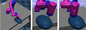
This case is similar to the task presented in [1]. The goal is to explore everywhere on the object surface (position control) with constant downward force (force control). We can directly apply the hybrid controller here with force in $z$ direction maintained. The process is also equivalent to contour tracking with constant force as shown in Fig. 3. In the simulation the object is an ellipsoid as shown in Fig. 3.

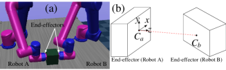
Using two arms to grab a box is a common task for human beings. To mimic this with robots, consider the scenario in which two robotic arms are used to grab a box as shown in Fig. 4 (a).

During the process, the end-effector of two robots have to track the pre-designed trajectories, and maintain a force in the $z$ direction of the frame with origin at $C_{a}$ as shown in Fig. 4 (b). Therefore a motion/force controller is needed. The proposed hybrid controller can be applied in this case through modifying the mapping $f$ in Eq. (3). Note that the hybrid controller will only be applied to robot B as shown in Fig. 4 (a) in order to establish an invertible and smooth mapping from the joint space to the task space as explained next. Robot A is controlled with a motion controller.

As seen in Fig. 4 (a), the frame ($C_{a}$ is the frame origin) attached to the end-effector of robot A can be determined with $\phi(t)=\{(x_{a}(t),y_{a}(t),z_{a}(t)),[V_{x}(t),V_{y}(t),V_{z}(t)]\}$, where $(x_{a}(t),y_{a}(t),z_{a}(t))$ is the coordinate of $C_{a}$ in world frame and $[V_{x}(t),V_{y}(t),V_{z}(t)]^{T}\in\mathbb{R}^{3\times 1}$ represents the directions of the $x$, $y$, and $z$ axes of the attached frame in world frame. Note that once the trajectory of end-effector of robot A is given, $\phi(t)$ is fixed at time $t$ assuming the motion controller works effectively. Recall that the aforementioned mapping $f:{\bm{\theta}}\in Q\to\bm{x}\in\mathbb{R}^{6\times 1}$ with $\bm{x}=[\alpha,\beta,\gamma,x,y,z]^{T}$. Now for the end-effector of robot B, define a new mapping $h:\bm{x}\to\bar{\bm{x}}$ where $\bar{\bm{x}}=[\alpha,\beta,\gamma,\bar{x},\bar{y},\bar{z}]^{T}$ and $\bar{x},\bar{y},\bar{z}$ can be computed as follows.

$$\begin{bmatrix}\bar{x}\\ \bar{y}\\ \bar{z}\end{bmatrix}=\begin{bmatrix}V_{x}^{T}\\ V_{y}^{T}\\ V_{z}^{T}\end{bmatrix}\Bigg{(}\begin{bmatrix}x\\ y\\ z\end{bmatrix}-\begin{bmatrix}x_{a}\\ y_{a}\\ z_{a}\end{bmatrix}\Bigg{)}$$

(21)

It can be verified that $h$ is a smooth and invertible mapping. Therefore, $h\circ f$, the composition of two smooth and invertible mappings, is still a smooth and invertible mapping. Essentially, $h$ maps the coordinate of $C_{b}$ to the frame originated at $C_{a}$. Thus the force in the $z$ direction of frame $C_{a}$ is determined by $\bar{z}$ which is the same with the hybrid controller we discussed before. Therefore, the same hybrid controller can be applied by modifying the mapping from $f$ to $h\circ f$.

Note that this does not mean that the box is guaranteed to be picked up and follow the desired trajectory, the force-closure conditions are required to hold [2]. Here we assume that the force-closure conditions hold by adjusting properly the initial orientation and position of the two end-effectors as shown in Fig. 4 (a).

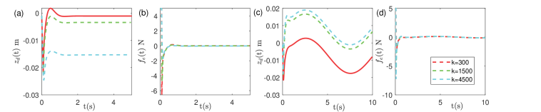
To simulate the force controller Eq. (9)-(10), parameters of controller Eq. (6) were set as $K_{v}=35$, $K_{p}=405$, and $K_{i}=1500$. The desired force was $f_{z}=5$N. The PI force controller parameters are $K_{p1}=-0.05$ and $K_{i1}=-0.01$. We simulated the contact model for three different spring constants: $k=300$N/m, $k=1500$N/m, and $k=4500$N/m. At the beginning, the tip position was $z_{t}=0.05$m. The initial desired position was $z_{d}=-0.001$m.

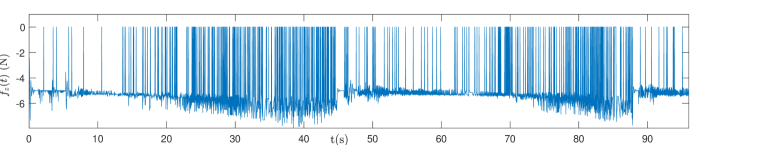
If $\epsilon=0$ and $\eta=0$, it can be checked that all the nonzero eigenvalues of $A_{w}$ have negative real parts, thus the above analysis can be applied. Fig. 5 (a) and (b) show the performance of the force controller for different $k$s when $q_{z}=0$. It can be seen that the system starts from non-contact mode and then switches to contact model and remains there for the rest time. The force can be accurately regulated for different $k$s and converges in about 0.1s.

To test the controller performance for time-varying $q_{z}$, we simulated the controller with $q_{z}(t)=0.01\sin(2\pi 0.2t)+0.01$m. The results are shown in Fig. 5(c) and (d). This can happen when the tip is sliding on a curved surface. It can be seen that the converged force error is very small for different $k$ even when the contact point changes from 0.02m to 0m in about 5s.

The robotic arm used is UR5 which has the size of a human arm and the simulation platform is MuJoCo [18]. For both two cases, the controller parameters are $K_{v}=35$, $K_{p}=405$, $K_{i}=1500$, $K_{p1}=0.008$ and $K_{i1}=0.002$. The video is available in the supplementary material.

In this case, the topography $q_{z}$ is changing as shown in Fig. 3. The force curve during the polishing process is shown in Fig. 6 (b) and the downward force is maintained to $-5$N.

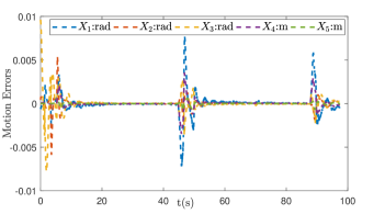
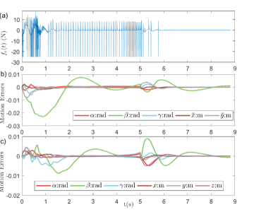
In this case, the goal is to lift the box with mass of 1kg and move along the vector $[0.27,0.1,0.27]$m within 5s in the world frame. Note that the hybrid controller is only applied to robotic arm B while the other one is controlled by a motion controller alone. The force is regulated to 20N with the friction coefficient set to be 0.9 and the force control error is shown in Fig. 8 (a). The motion control errors for the two robots are shown in Fig. 8 (b) and (c), respectively. Note that for robotic arm B the motion error are expressed in term of $\bar{x}$ and $\bar{y}$ based on the mapping in Eq. (21). Again, the hybrid controller works as expected with both the motion and force regulated.

Note that for both cases the force error is very noisy as can be seen in Figs. 6 and 8 (a). This is partly due to the fact that the environment in simulation is very hard. The contact is shortly broken and then established again due to the controller resulting in spikes in the plots. On the other hand, the algorithm for calculating the interaction force in MuJoCo may also contribute to this. Computing the interaction force is transformed to solving an optimization problem in MuJoCo making it very challenging to set parameters to change the elasticity of the environment.

References

- [1] C. Schindlbeck and S. Haddadin, “Unified passivity-based cartesian force/impedance control for rigid and flexible joint robots via task-energy tanks,” in 2015 IEEE International Conference on Robotics and Automation, pp. 440–447, IEEE, 2015.
- [2] K. M. Lynch and F. C. Park, Modern Robotics. Cambridge University Press, 2017.
- [3] R. M. Murray, Z. Li, S. S. Sastry, and S. S. Sastry, A mathematical introduction to robotic manipulation. CRC press, 1994.
- [4] N. Hogan, “Impedance control: An approach to manipulation: Part i—theory,” 1985.
- [5] C. Ott, R. Mukherjee, and Y. Nakamura, “Unified impedance and admittance control,” in 2010 IEEE International Conference on Robotics and Automation, pp. 554–561, IEEE, 2010.
- [6] F. Lange, W. Bertleff, and M. Suppa, “Force and trajectory control of industrial robots in stiff contact,” in 2013 IEEE International Conference on Robotics and Automation, pp. 2927–2934, IEEE, 2013.
- [7] T. Kroger, B. Finkemeyer, M. Heuck, and F. M. Wahl, “Adaptive implicit hybrid force/pose control of industrial manipulators: Compliant motion experiments,” in 2004 IEEE/RSJ International Conference on Intelligent Robots and Systems(IEEE Cat. No. 04CH37566), vol. 1, pp. 816–821, IEEE, 2004.
- [8] S. A. M. Dehghan, M. Danesh, and F. Sheikholeslam, “Adaptive hybrid force/position control of robot manipulators using an adaptive force estimator in the presence of parametric uncertainty,” Advanced Robotics, vol. 29, no. 4, pp. 209–223, 2015.
- [9] M. H. Raibert and J. J. Craig, “Hybrid position/force control of manipulators,” 1981.
- [10] J. Duffy, “The fallacy of modern hybrid control theory that is based on “orthogonal complements” of twist and wrench spaces,” Journal of Robotic systems, vol. 7, no. 2, pp. 139–144, 1990.
- [11] A. G. Marin and R. Weitschat, “Unified impedance and hybrid force-position controller with kinestatic filtering,” in 2016 IEEE/RSJ International Conference on Intelligent Robots and Systems, pp. 3353–3359, IEEE, 2016.
- [12] V. Duindam and S. Stramigioli, “Port-based asymptotic curve tracking for mechanical systems,” European Journal of Control, vol. 10, no. 5, pp. 411–420, 2004.
- [13] C. T. Landi, F. Ferraguti, C. Fantuzzi, and C. Secchi, “A passivity-based strategy for coaching in human-robot interaction,” in 2018 IEEE International Conference on Robotics and Automation, pp. 1–6, IEEE, 2018.
- [14] S. Chen, Z. Wang, A. Chakraborty, M. Klecka, G. Saunders, and J. Wen, “Robotic deep rolling with iterative learning motion and force control,” IEEE Robotics and Automation Letters, vol. 5, no. 4, pp. 5581–5588, 2020.
- [15] G. Liu, L. Fang, B. Han, and H. Zhang, “Frequency-division based hybrid force/position control of robotic arms manipulating in uncertain environments,” Industrial Robot: the international journal of robotics research and application, 2020.
- [16] C.-T. Chen, Introduction to linear system theory. Holt, Rinehart and Winston, 1970.
- [17] H. K. Khalil and J. W. Grizzle, Nonlinear systems, vol. 3. Prentice hall Upper Saddle River, NJ, 2002.
- [18] E. Todorov, “Convex and analytically-invertible dynamics with contacts and constraints: Theory and implementation in mujoco,” in 2014 IEEE International Conference on Robotics and Automation, pp. 6054–6061, IEEE, 2014.
- [19] S. Xie, “Mounting a screwdriver onto a screw using hybrid control,” Master’s thesis, Iowa State University, USA, 2020.